Real space inhomogeneities in high temperature superconductors: the perspective of two-component model

Abstract

The two-component model of high temperature superconductors in its real space version has been solved using Bogoliubov-de Gennes equations. The disorder in the electron and boson subsystem has been taken into account. It strongly modifies the superconducting properties and leads to local variations of the gap parameter and density of states. The assumption that the impurities mainly modify boson energies offers natural explanation of the puzzling positive correlation between the positions of impurities and the values of the order parameter found in the scanning tunnelling microscopy experiments.

1 Introduction

Recent years have witnessed the interesting series of experiments on high temperature superconductors (HTS). These include inter alia scanning tunnelling spectroscopy measurements which revealed atomic scale inhomogeneities on the surface of BiSrCaCuO [1, 2, 3, 4, 5] and the quantum oscillations [6, 7, 8] which are signatures of the well developed Fermi surface. All these discoveries clearly indicate that after more than 20 years of research, high temperature superconductors (HTS) still present a challenge and are the objects of intensive experimental [9, 10, 11, 12] and theoretical studies [13, 14, 15, 16].

The scanning tunnelling microscopy (STM) experiments are mainly performed on Bi family of HTS [17]. These materials cleave easily and it is straightforward to obtain atomically clean surfaces predominantly with BiO surface layer. This makes Bi superconductors also interesting materials to study by means of angle-resolved photoemission spectroscopy (ARPES) [9]. The strength of STM technique consists in its high energetic and spatial resolution. With STM one is able to study changes of local properties within the atomic distances. The poor screening, short superconducting coherence length of cuprate superconductors and low-dimensionality of the electronic structure contribute to large spatial fluctuations in normal and superconducting state properties.

STM measures the quasiparticle excitations, existing at a given energy. From the differential conductance spectra one deduces e.g. local values of superconducting gap. The study of HTS reveals a number of unexpected features in the STM spectra. Among those “universally” observed there was nearly a homogeneous structure of conductance spectra at low energies despite strong variations at higher energies and in particular, inferred gap values [3], the asymmetry (i.e. $G(-V)\neq G(V)$) of the differential conductance [18] $G(V)=dI/dV$ and characteristic dip-hump structure [19].

Already in the early days of HTS, the measured STM spectra have shown high degree of disorder [20, 21]. The subsequent more precise experiments allowed for the analysis of the results not only in real, but also in reciprocal space. It is important to note that with the Fourier transformed STM data, the possibility appeared to reconstruct the energy gap $\Delta({\bf k})$, which turned out to be in agreement [22] with the ARPES measurements. The study of the spatial maps resulted in discovery that the values of the superconducting gaps are positively correlated with positions of oxygen dopants thus supporting the earlier claims that electronic inhomogeneities and atomic disorder are interrelated. Since then inhomogeneities are thus commonly attributed to the presence of disorder [23].

The development [24] of the so called “lattice-tracking spectroscopy” has enabled investigation of various correlations between the local system properties even at significantly different temperatures. This resulted in finding that not only the positions of dopant oxygen atoms correlate [5, 25] with local values of the superconducting gap, but that also the latter property is positively correlated with local density of states (LDOS) measured in the normal state at a temperature well above that of the superconducting transition. This correlation indicates that normal state contains information about the interactions responsible for superconducting instability of the system [26].

The purpose of this paper is to study theoretically local properties of HTS relevant to the STM experiments. We describe the superconductor by the two-component boson-fermion (BF) model [27, 28]. For the homogeneous system the Hamiltonian can be written as

$${\hat{\cal H}}^{{BF}} = \sum_{\vec{k},\sigma}(\varepsilon(\vec{k})-\mu)\hat{c}_{\vec{k}\sigma}^{\dagger}\hat{c}_{\vec{k}\sigma}+\sum_{\vec{q}}\left(E_{\vec{q}}^{B}-2\mu\right)\hat{b}_{\vec{q}}^{\dagger}\hat{b}_{\vec{q}}$$ (1)

$$+ \frac{1}{\sqrt{N}}\sum_{\vec{k},\vec{q}}g_{\vec{k},\vec{q}}\left(\hat{b}_{\vec{q}}^{\dagger}\hat{c}_{\vec{q}-\vec{k}\downarrow}\hat{c}_{\vec{k}\uparrow}+\hat{c}_{\vec{k}\uparrow}^{\dagger}\hat{c}_{\vec{q}-\vec{k}\downarrow}^{\dagger}\hat{b}_{\vec{q}}\right).$$

The $c_{\vec{k}}(c_{\vec{k}}^{\dagger})$ operators refer to single fermions and annihilation (creation) operators of bosons are denoted by $b_{\vec{q}}(b_{\vec{q}}^{\dagger})$. The d-wave character of the order parameter in superconducting state is taken into account by assuming for two dimensional lattice $g_{\vec{k}}=g[\cos(k_{x}a)-\cos(k_{y}a)]$.

Coexisting local pairs (bosons) and electrons are described by the Hamiltonian (1) which has been proposed on phenomenological basis [27] but can also be derived from generalized periodic Anderson model [28] or as a low energy limit of cluster states [29]. Its relevance to HTS and other unconventional superconductors has been demonstrated in numerous works of various groups [30, 31, 32, 33, 34, 35, 36, 37, 38, 39, 40, 41, 42]. In a broader context this phenomenological two-component pairing scenario plays a role in a great variety of different physical situations. (i) It applies to resonant pairing in cold atomic fermion gases via a Feshbach resonance [43], (ii) it captures the salient features of Anderson’s resonating valence bond scenario [29] and (iii) it permits to draw conclusions about the pairing mechanism, if given by local dynamical lattice fluctuations, as was the original motivation for proposing this model [27].

As in this work we are concerned with the description of inhomogeneities and correlations observed experimentally, we generalize the Hamiltonian (1) to the real space and make the parameters random numbers. It means that disorder is responsible for various kinds of inhomogeneities. In the absence of ab-intio calculations [29] of how the boson and fermion parameters behave in an impure system [44] we study a few scenarios of their possible changes.

It should be stressed that we are not averaging over disorder as experiments measure local values for a given (fixed) configuration. It turns out that with the BF model a number of experimental correlations found in STM can be understood with reasonable assumptions about the role of disorder. Here we shall be mainly interested in the maps of local density of states, the shapes of differential conductance curves as the functions of energy (applied bias) as measured at different sites and the values of energy gaps. Preliminary studies of this model have been presented recently [45]. In literature there exist numerous attempts to describe theoretically various aspects of the STM spectra in HTS cuprates including inter alia inhomogeneities [46, 47, 48, 49, 50, 51], asymmetry of the differential conductance [52] and dip-hump structures [53].

The organization of the rest of the paper is as follows. In section 2 we introduce the two-component model, discuss the approach and compare the calculations for a small homogeneous system with bulk one. The results for the model with disorder in the electron and boson subsystems are presented in section 3 whereas main conclusions in section 4.

2 The model and approach

We start with the two-component model in a real space where fermions interact via short range forces with the hard-core charged and localized bosons. This boson-fermion model [28, 41] is represented by the Hamiltonian

$${\hat{\cal H}}^{{BF}} = \sum_{i,j,\sigma}t_{ij}\hat{c}_{i\sigma}^{\dagger}\hat{c}_{j\sigma}+\sum_{i\sigma}\left(V_{i}^{{imp}}-\mu\right)\hat{c}_{i\sigma}^{\dagger}\hat{c}_{i\sigma}+\sum_{i}\left(E_{i}^{B}-2\mu\right)\hat{b}_{i}^{\dagger}\hat{b}_{i}$$ (2)

$$+ \sum_{i,j}\frac{g_{ij}}{2}\left[\hat{b}_{i}^{\dagger}(\hat{c}_{i\downarrow}\hat{c}_{j\uparrow}-\hat{c}_{i\uparrow}\hat{c}_{j\downarrow})+\hat{b}_{i}(\hat{c}_{j\uparrow}^{\dagger}\hat{c}_{i\downarrow}^{\dagger}-\hat{c}_{j\downarrow}^{\dagger}\hat{c}_{i\uparrow}^{\dagger})\right],$$

where $i$ and $j$ denote the lattice sites, $\hat{c}_{i,\sigma}^{\dagger}$ ($\hat{c}_{i,\sigma}$) stand for creation (annihilation) operator of fermion at the site $i$ with spin $\sigma$. $\hat{b}_{i}^{\dagger}$ and $\hat{b}_{i}$ are the creation and annihilation operators of hard-core bosons at the site $i$. $\mu$ stands for the chemical potential of the system and $t_{ij}$ are hopping integrals. $g_{ij}$ is the electron-boson scattering (charge exchange). $V^{imp}_{i}$ is the local value of the fermionic energy level (scattering potential due to impurities) and $E^{B}_{i}$ denotes the position of the bosonic level. We shall discuss the systems on a square lattice with hopping parameters between the nearest neighbors to be denoted $t$, which we use as the energy unit.

2.1 Bogoliubov - de Gennes equations

To account for the short coherence length and d-wave symmetry of the superconducting order parameter we assume that the boson-fermion coupling $g_{ij}$ takes on non-zero value for the nearest neighbor sites $<i,j>$ only and equals +g if $j=i\pm\vec{x}$ and -g if $j=i\pm\vec{y}$.

Application of the standard Hartree-Fock-Bogoliubov decoupling of the type $\hat{b}_{i}^{\dagger}\hat{c}_{i\downarrow}\hat{c}_{j\uparrow}\approx\langle\hat{b}_{i}^{\dagger}\rangle\hat{c}_{i\downarrow}\hat{c}_{j\uparrow}+\hat{b}_{i}^{\dagger}\langle\hat{c}_{i\downarrow}\hat{c}_{j\uparrow}\rangle$ leads to $\hat{H}^{{BF}}=\hat{H}^{{B}}+\hat{H}^{{F}}$, where $\hat{H}^{{B}}$ is the single site bosonic Hamiltonian

$$\hat{H}^{{B}}=\sum_{i}\left(E_{i}^{B}-2\mu\right)\hat{b}_{i}^{\dagger}\hat{b}_{i}+\sum_{i}\left(\hat{b}_{i}^{\dagger}\chi_{i}+\hat{b}_{i}\chi_{i}^{*}\right)$$ (3)

with the parameter $\chi_{i}=\displaystyle\sum_{<j>}(g_{ij}/2)<\hat{c}_{i,\downarrow}\hat{c}_{j,\uparrow}-\hat{c}_{i,\uparrow}\hat{c}_{j,\downarrow}>$ depending on the fermionic degrees of freedom. $\hat{H}^{{F}}$ is the Hamiltonian describing the disordered fermionic subsystem [54].

$$\hat{H}^{{F}} = \sum_{i,j,\sigma}t_{ij}\hat{c}_{i\sigma}^{\dagger}\hat{c}_{j\sigma}+\sum_{i\sigma}\left(V_{i}^{{imp}}-\mu\right)\hat{c}_{i\sigma}^{\dagger}\hat{c}_{i\sigma}$$

$$+ \sum_{i,j}\left[\Delta_{ij}^{*}(\hat{c}_{i\downarrow}\hat{c}_{j\uparrow}-\hat{c}_{i\uparrow}\hat{c}_{j\downarrow})+\Delta_{ij}(\hat{c}_{j\uparrow}^{\dagger}\hat{c}_{i\downarrow}^{\dagger}-\hat{c}_{j\downarrow}^{\dagger}\hat{c}_{i\uparrow}^{\dagger})\right].$$

The standard statistical approach allows for an exact solution of the boson Hamiltonian $\hat{H}^{{B}}$. For a given realization of disorder one finds the following equations for the local number of bosons $<\hat{b}_{i}^{\dagger}\hat{b}_{i}>$ and the local boson average $<\hat{b}_{i}>$

$$<\hat{b}_{i}^{\dagger}\hat{b}_{i}> = \frac{1}{2}-\frac{E_{i}^{B}-2\mu}{4\epsilon_{i}}\tanh\left(\frac{\epsilon_{i}}{k_{B}T}\right),$$ (5)

$$<\hat{b}_{i}> = -\frac{\chi_{i}}{2\epsilon_{i}}\tanh\left(\frac{\epsilon_{i}}{k_{B}T}\right).$$ (6)

We have denoted $\epsilon_{i}=\sqrt{\left(\frac{E^{B}_{i}-2\mu}{2}\right)^{2}+|\chi_{i}|^{2}}$ and $\Delta_{ij}=g_{ij}<\hat{b}_{i}>$/2. It is $\Delta_{ij}$ which couples two subsystems as follows from equation (14) below.

The fermion part has the standard BCS-structure and we diagonalize it by the Bogoliubov-Valatin transformation, which introduces the new quasiparticle operators [55] $\hat{\gamma}_{l,\downarrow},\hat{\gamma}_{l,\uparrow}$ and their adjoint counterparts $\hat{\gamma}^{\dagger}_{l,\downarrow},\hat{\gamma}^{\dagger}_{l,\uparrow}$

$$\hat{c}_{i,\downarrow}=\sum_{l}\left[u_{i}^{l}\hat{\gamma}_{l,\downarrow}+v^{l*}_{i}\hat{\gamma}^{\dagger}_{l,\uparrow}\right],$$ (7)

$$\hat{c}_{i,\uparrow}=\sum_{l}\left[u_{i}^{l}\hat{\gamma}_{l,\uparrow}-v^{l*}_{i}\hat{\gamma}^{\dagger}_{l,\downarrow}\right].$$

This yields the following Bogoliubov-de Gennes equations [45, 54]

$$\sum_{j}\left(\begin{array}[]{c}t_{ij}+\left(V_{i}^{{imp}}-\mu\right)\delta_{ij};\tilde{\Delta}_{ij}\\ \tilde{\Delta}_{ij}^{*};-t_{ij}-\left(V_{i}^{{imp}}-\mu\right)\delta_{ij}\end{array}\right)\left(\begin{array}[]{r}u^{l}_{j}\\ v^{l}_{j}\end{array}\right)=E^{l}\left(\begin{array}[]{c}u^{l}_{i}\\ v^{l}_{i}\end{array}\right),$$ (14)

with $\tilde{\Delta}_{ij}=\Delta_{ij}+\Delta_{ji}$. For a given value of the chemical potential $\mu$ one solves the system of equations (14) self-consistently together with (6) for the energies $E^{l}$ and the functions $u^{l}_{i},v^{l}_{i}$. For a system on a square lattice of $n\times m$ sites the size of the matrix is $(2nm)^{2}$. If the total carrier concentration $n=n_{f}+2n_{b}$ is fixed, one finds $\mu$ from

$$n={1\over N}\sum_{i\sigma}\langle\hat{c}_{i\sigma}^{\dagger}\hat{c}_{i\sigma}\rangle+{2\over N}\sum_{i}<\hat{b}_{i}^{\dagger}\hat{b}_{i}>$$ (15)

and using equations (5-6) and (17).

The solutions enable calculation of all parameters of interest. In particular the local density of states (LDOS) $N(E,i)$ at the site $i$ as a function of energy $E$ is given by

$$N(E,i)=\sum_{l}\left[|u^{l}_{i}|^{2}\delta(E-E^{l})+|v^{l}_{i}|^{2}\delta(E+E^{l})\right].$$ (16)

For the purpose of numerical calculations we shall replace the Dirac $\delta(E)$ distribution by the Lorentzian ${{1}\over{\pi}}{{\eta}\over{E^{2}+\eta^{2}}}$, with $\eta$ being a small smearing parameter. The local fermion number density $n_{f,i}=n_{f}(\vec{R}_{i})=\sum_{\sigma}\langle c^{+}_{i\sigma}c_{i\sigma}\rangle$ is found to be

$$n_{f,i}=\sum_{l}\left[|u^{l}_{i}|^{2}f(E^{l})+|v^{l}_{i}|^{2}(1-f(E^{l}))\right],$$ (17)

where $f(E^{l})=1/[\exp(E^{l}/k_{B}T)+1]$ is the Fermi-Dirac distribution function. Parameter $\chi_{i}$ is given by

$$\chi_{i}=\displaystyle\sum_{l}\sum_{<j>}g_{ij}\left[-u^{l}_{i}v^{l*}_{j}(1-f(E^{l}))+u^{l}_{j}v^{l*}_{i}f(E^{l})\right].$$ (18)

The above equations are general in a sense that they allow for the study of both s-wave and d-wave superconductors depending on the choice of coupling $g_{ij}$. For the d-wave symmetry we define the local value of the order parameter at the site $i$ as the staggered sum [50] over the neighboring bonds $j$,

$$\Delta_{i}=(-\tilde{\Delta}_{i,i+y}+\tilde{\Delta}_{i,i+x}-\tilde{\Delta}_{i,i-y}+\tilde{\Delta}_{i,i-x})/4.$$ (19)

The correlation function $C_{f,h}$ between various parameters $f,h$ (in fact, also depending on the points of our lattice $f_{i}$ and $h_{i}$) is defined as [49]

$$C_{f,h}\left(R\right)=\frac{\displaystyle\sum_{i}\sum_{j}\left(f_{i}-f_{average}\right)\left(h_{j}-h_{average}\right)}{\displaystyle\sqrt{\sum_{i}\left(f_{i}-f_{average}\right)^{2}}\sqrt{\sum_{i}\left(h_{i}-h_{average}\right)^{2}}},$$ (20)

where $f_{average}$ and $h_{average}$ are their values averaged over all sites and $R=|i-j|$ is the fixed distance between the sites $i$ and $j$ in the above summations.

In the next subsection we first recall the main features of the homogeneous boson - fermion model (1) and compare the results for a small cluster with those for the bulk homogeneous system.

2.2 Clean system

We consider here a real space version of the BF model and solve the corresponding Bogoliubov - de Gennes equations first for the homogeneous system of finite size with the periodic boundary conditions and compare the results with those obtained for the bulk system for the same set of parameters. This serves as a check of the quality of calculations for a relatively small size of the system.

Figure 1 shows the dependence of the zero temperature order parameters $\left<b\right>$, $|\chi|$ and the corresponding energy gap $\Delta$ (upper-left panel), the critical temperature $T_{c}$ (upper-right panel) and their ratio $2\Delta/T_{c}$ (bottom left panel) on the boson energy level $E^{B}$ measured with respect to the chemical potential. In the upper right panel the solid curve represents the data for the bulk homogeneous system, whereas the crosses show the results for the finite cluster. These data obtained for d-wave superconductor by solving the Bogoliubov - de Gennes equations for the very small system of size $17\times 21$ sites and the periodic boundary conditions agree very well with the results obtained from the mean-field study of the two- dimensional square lattice in the thermodynamic limit [41].

Small deviations are visible for $E^{B}\gtrsim t$, when real space calculations give slightly larger values. These are due to the finite size effect. Let us recall that the spectrum of a small system is discrete and usually highly degenerate. The degree of degeneracy, however, is substantially reduced if one chooses rectangular shape of the system. This reduces number of symmetries in the Bogolubov-de Gennes equations and lowers degeneracy of energies. Best agreement with the bulk data is obtained for lengths $n$ and $m$ being different prime numbers.

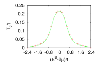
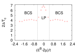
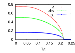
Figure 1: (Colour online) The local order parameters $<b_{i}>$, $|\chi_{i}|$ and ($\Delta_{i}$) at $T$=$0$ in the units t (upper left panel), superconducting transition temperature ($T_{c}/t$) (upper right panel) and their ratio $2\Delta/T_{c}$ (lower left panel) are plotted as the functions of the boson energy $(E^{B}-2\mu)/t$ for a small, homogeneous system of the size $17\times 21$ with $g$=$0.375t$, $\mu$=$0.0t$, $V^{imp}$=$0.0t$. The lower right panel shows the dependence of various (coupled) order parameters on temperature for $E^{B}$=$2\mu$. The superconducting transition temperature (crosses) obtained here is compared with that calculated for the corresponding bulk system (dotted curve).

We remark that the quantities plotted in Figure 1 are symmetric with respect to $E^{B}-2\mu=0$. Physically this property comes from the hard-core nature of the local pairs (LP). Upon filling the bosonic level we obtain a perfect particle-hole symmetry between $n^{B}$ and $1-n^{B}$ occupancies. If $\mu=0$ both these cases equally promote the superfluid/superconducting abilities of the coupled boson-fermion system (2). In particular, let us notice strong enhancement of the critical temperature near the half-filled boson level which is accompanied by the non-BCS relation $2\Delta/T_{c}$ (marked in lower left panel of Fig. 1 as LP) being a hallmark of the present scenario [27].

The model shows superfluid characteristics which are intermediate between those of a BCS regime and those of local bipolaronic pairs [30, 56]. For the homogeneous case, the effective interaction $I_{0}^{eff}$ between fermions depends on the boson-fermion coupling $g$, the position of the bosonic energies $E^{B}$ with respect to the chemical potential and hard-core boson concentration $n_{B}$ as $I_{0}^{eff}=(g^{2}/(E^{B}-2\mu))(1-2n_{B})$. This can be easily seen [39, 41] by rewriting equations (6) -(14) for the clean bulk system in the form of effective BCS equation for the fermionic order parameter. The coupling $g_{ij}$ induces BCS like pairing in the fermionic subsystem and the Bose-Einstein condensation (BEC) in the bosonic subsystem. The inherent property of the model is that superconductivity vanishes at the same temperature $T_{c}$ in both subsystems [42]. Temperature dependencies of the bosonic $|<\hat{b}>|$, fermionic $|\chi_{i}|$ and $\Delta_{i}$ order parameters of the clean system are shown in the lower right panel of Figure 1.

For the vanishing boson-fermion coupling $g_{ij}=0$ model (2) describes the two non-interacting subsystems; dirty fermions and immobile hard-core bosons in random potential. None of the subsystems taken alone undergoes the transition.

2.3 Remarks on the phase diagram of HTS

The undoped parent compounds of cuprate HTSs are characterized by a non-superconducting ground state, which is antifferromagnetic insulator. With the increasing doping the system starts to be metallic and superconducting. The superconducting transition temperature T_c increases with increasing doping, attains a maximal value for the optimal doping and decreases again in the overdoped regime. At the same time the normal state properties change dramatically. The pseudogap state [57], which sets in at small doping disappears and the overdoped system might behave as normal Fermi liquid. The doping is on the one hand the source of charge carriers in the model, while on the other hand it introduces impurities. Judging from the appearance of superconductivity for finite impurity concentration the plausible assumption would be that impurities modify local values of the parameters in the Hamiltonian (2) in such a way as to promote superconductivity.

We thus assume that oxygen impurities in HTS are the source of carriers (holes) and disorder in the system. The previous studies of the disordered boson-fermion model concentrated on the bulk properties and required the averaging over configurations. This was achieved by averaging the free energy [58] or using the coherent potential approximation to calculate the averaged Green functions [54, 59]. The role of disorder is hard to overestimate in these materials. It seems that most of their unusual properties may simply be due to an unprecedented degree of disorder resulting from both potential scattering and random values of other parameters. The simultaneous presence of strong correlations in real materials makes the problem more complicated [60] even at the mean field level [61].

In the two-component model it is the boson-fermion scattering which induces superconducting transition. In this scenario the pseudogap phase is dominated by the incoherent pairs of bosonic character. To model the initial increase of the superconducting transition temperature with doping we assume that dopants modulate bosonic levels $E_{i}^{B}$ changing them locally from the value well below or above the Fermi level to its vicinity which allows for efficient fermion-boson scattering and superconducting instability. The proper choice of $E_{i}^{B}$ leads to positive correlations between the positions of impurities and the amplitude of the gap in the local density of states.

3 Results of calculations

The description of the cuprate superconductors by the disordered boson-fermion model (2) allows for a great variety of scenarios. In the following we shall consider a number of them as our main goal here is to look at various possibilities offered by the model at hand.

We numerically solve the Bogoliubov-de Gennes equations for small clusters with the size $n\times m$ sites. We use periodic boundary conditions, with which the solutions converge to the correct bulk values, even for a relatively small system. We determine the values of the order parameter $\Delta_{ij}$ for the d-wave superconductivity at each bond $i-j$, the carrier concentration $n_{i}=n(\vec{r}_{i})$ at each site and the local density of states $N(E,i)$. The results are presented in the form of maps showing these local parameters. For the d-wave order parameter we shall use the local “representation” of $\Delta_{ij}$ as given by equation (19). In this work we limit the discussion to the analysis of the ground state ($T=0K$) properties. In the following we shall compare our results with STM data taken at low temperatures. Because the energy gap changes very slowly for temperatures T¡0.3$T_{c}$, as it is visible in Fig. 1 the ground state data can safely be compared with the experiment

As mentioned before, the model and approach allow us to study various kinds of inhomogeneities. They may result from the local changes of:

– $E_{i}^{B}$, the position of the boson energy level. As we know from the study of the model for the clean system, the position of $E_{i}^{B}$ with respect to the chemical potential has a profound effect on the appearance of superconductivity.

– $V_{i}^{imp}$, which can be interpreted as local atomic levels. This term represents the scattering of fermions by point impurities.

– $t_{ij}$, the fluctuating values of hopping parameters. The fluctuations of this type are not discussed in this paper.

3.1 Random bosonic levels supporting or suppressing superconductivity

It is the experimental fact that undoped copper oxides are not superconducting. As noted above, the existence of coupling between the subsystems $g_{ij}$ causes superconducting instability. It is also evident from Figure 1 that for superconductivity to appear the bosonic levels $E^{B}_{i}$ have to be close enough to the Fermi level. It seems thus natural to expect that doping of parent compounds introduces carriers into the system and places the boson levels in the close vicinity to the Fermi energy. In accordance with such a picture we study here a few different (model) scenarios of doping.

First, we consider random $E^{B}_{i}$ centers, which we also call impurities with parameter values supporting superconductivity. It means they move locally the boson level towards the Fermi level (c.f. upper panel of Figure 1). Second case is another extreme in which contrary to the above expectations impurities move the boson level out of its initial position in the close vicinity of $\mu$ and push it up or down on the energy scale. This makes the boson-fermion scattering ineffective due to phase space restrictions. In this scenario $E^{B}_{i}$ impurities suppress superconductivity.

The above two scenarios neglect the effect of disorder on the fermion subsystem i.e. we put $V_{i}^{imp}=0$. In real systems one expects that the centers with the boson levels closer to the Fermi energy, at the same time are the source of (presumably strong) potential scattering for fermions, which in our system is modelled by $V^{imp}$. Thus as the third scenario we consider the system in which the doping will introduce randomness in both boson and electron on-site parameters. In order not to increase a number of parameters we assume [62] that in this case the relation $E^{B}_{i}=2V_{i}$ and $V^{imp}=V_{i}$ is valid.

It has to be stressed that in principle there exists an additional degree of freedom which is related to the spatial extent [50] at which introduction of the impurity into the lattice will modify the parameters of the effective model as (2). Accordingly we discuss short (local) and long range (extended) impurities. In the latter case the impurity at a given site will modify the boson energy levels in neighboring and more distant sites (see Figs. 2-6). If two extended impurities happen to influence the same site their effects simply add up.

In Figure 2 we show a superconducting system with relatively low transition temperature and introduce local impurities which move the boson levels $E^{B}_{i}$ towards the chemical potential, thus increasing $T_{c}$. Next two figures (i.e. Figure 3 and 4) refer to the extended impurities. The maps of the local order parameter $\Delta_{i}$ of the d-wave superconductor are shown in the upper left panels.

The upper right panels of Figures 3 and 4 show the distance $R$ dependence of the correlation functions $C_{f,h}$, as defined in Eq. (20), for the following parameters ($f,h$):

(i) local values of the fermionic order parameter $\Delta_{i}$ with positions of the impurities; $R^{imp}$,

(ii) local values of bosonic order parameter $\langle b_{i}\rangle$ with $R^{imp}$

(iii) $\Delta_{i}$ with the maximal height of the local density of states $N(i)$ denoted as LDOS^peak in the figures. Note, that at each lattice site the height of $N(i,\omega)$ is the largest at slightly different energy $\omega$.

(iv) the correlation of $\Delta_{i}$ with its value at the distance $i+R$. The extent of this correlation can be viewed as a measure of the coherence length $\xi$. For the short range impurities it is of the order of one lattice spacing and increases with the range of effective interaction.

The STM spectra shown as the functions of energy (bias) in Fig. 2 are taken along vertical line at $X=53$ (left) and $X=67$ (right), whereas those in Fig. 3 are for $X=17$ and $X=43$, respectively. The size of the system is $71\times 77$ and there are 16% of impurities (marked by circles) which change the boson levels $E^{B}_{i}$ locally from the homogeneous value 0.58t to 0t (Fig. 2). Other parameters of this d-wave superconductor are $t_{1}=1.0t$, $g=0.5t$, $V_{i}^{imp}=0$, and the total number of carriers $n=1.30$.

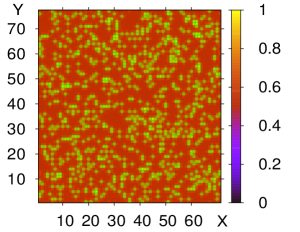
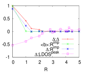
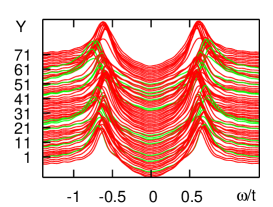
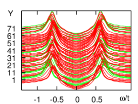
Figure 2: (Colour online) Map of the local order parameter $\Delta_{i}/t$ (upper left panel), the dependence of the correlation functions $C_{f,h}$ (upper right panel), the STM spectra taken along vertical line at $X$=$53$ (lower left) and $X$=$67$ (lower right panel). The size of the system is $71\times 77$ and there are $16\%$ of impurities (marked by circles) which change the boson levels $E^{B}_{i}$ locally from the homogeneous value $0.58t$ to $0t$. The other parameters of this d-wave superconductor are $g$=$0.5t$, $V_{i}^{imp}$=$0$, and the total number of carriers $n$=$1.3$.

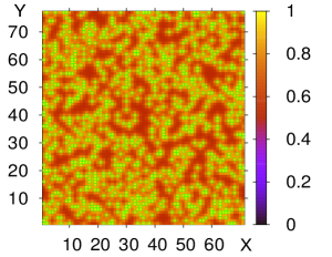
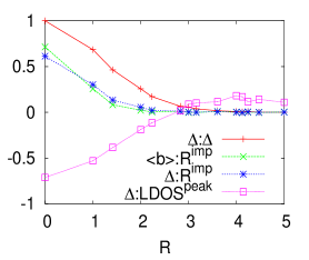
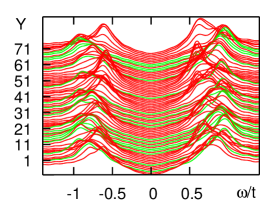
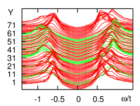
Figure 3: (Colour online) The same dependencies as in Figure 2 but LDOS is presented for $X$=$17,43$. We consider here the extended impurities which influence the positions of $E^{B}_{i}$ levels of neighboring sites changing them from the homogeneous value $0.58t$ to $0t$ at the impurity site, $0.29t$ at its nearest neighbor site, $0.425t$ and $0.5t$ at still further sites.

It has to be noted that even without impurities the homogeneous system with the above parameters is superconducting. These additional impurities increase its $T_{c}$. They also change the values of the local gaps, which are visible in the energy dependence of the local densities of states.

The correlation between the position of the impurities and amplitudes of the local order parameters $\Delta_{i}$ and $\left<b_{i}\right>$ in Fig. 2 is positive and short ranged. It is important to note slight differences between the two correlations which are related to strictly local nature of the bosonic order parameter $\left<b_{i}\right>$ and a longer range of the fermionic one. The summation of $\Delta_{ij}$ over the sites $j$ neighboring $i$ to get $\Delta_{i}$ makes the two local order parameters differ. The point-like character of effective interaction is responsible for the non monotonous dependence of these correlations on the distance. It is smooth for the more realistic case of longer range impurities shown in Figures 3 and 4.

The correlations between the local densities of states (at highest values) and the values of $\Delta_{i}$ are negative. These quantities are anti-correlated. This is true for both local, Figure 2, and extended Fig. 3 impurities. The correlation virtually vanishes (Fig. 4) for the same kind of extended impurities introduced into non-superconducting system which is here modelled by the position of bosonic levels very distant $E^{B}=4t$ from the Fermi energy (cf. upper left panel in figure (1)).

The anti-correlation is easy to understand. Close examination of the data indicates that each time LDOS is measured for a site where the order parameter is large, the coherence peaks are relatively broad, whereas they are sharp and high in the places with very low or even zero value of the order parameter. For the interpretation of the experiments this finding means that each time the STM tip is scanning the region of low (or even zero) order parameter it finds sharper edges of the spectra and lower apparent gap (defined as the peak to peak distance in the local density of states). On the contrary, the spectra calculated for the patches of the sample with large values of the order parameters display less sharp coherence features.

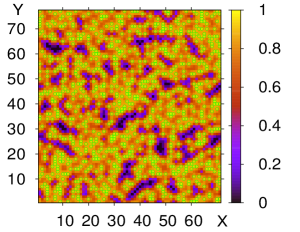
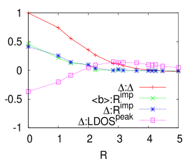
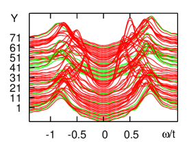
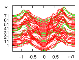
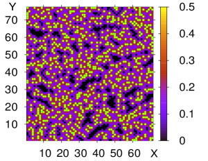
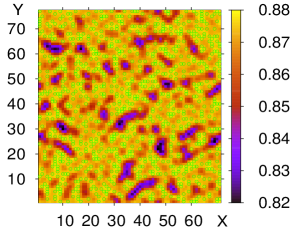
Figure 4: (Colour online) Effect of extended impurities on the non-superconducting system with $E^{B}_{i}$=$4t$. The same dependencies as in Figure 3 except LDOS are shown for $X$=$26,33$ and the lower panels show the maps of carrier concentration: bosons (left), and fermions (right). The total carrier concentration is kept constant $n$=$1.3$. The size of the system is $71\times 77$ and there are $16\%$ of impurities (marked by circles on the map of $\Delta_{i}/t$) which change the boson levels $E^{B}_{i}$ from the homogeneous value $4t$ to $0t$ at the impurity site, $0.29t$ at its nearest neighbor site, $0.425t$ and $0.5t$ at still further sites.

These sharp coherence-like features observed at the sites with low values of “effective” interactions $I_{i}^{eff}$ resemble those found in the nonsuperconducting region placed inside the superconductor [63] and induced by the proximity effect. We believe that the same general mechanism of proximity is operating here on the local scale and between regions with different values of the order parameters.

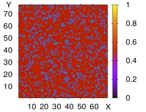
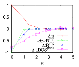
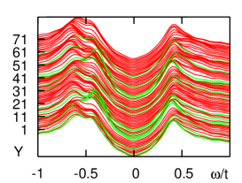
Figure 5: (Colour online) Map of the local gap $\Delta_{i}/t$ (upper left panel), the dependence of the correlation functions $C_{f,h}$ (upper right panel), the STM spectra taken along the vertical line at $X$=$29$ (lower left panel) and $X$=$39$ (lower right panel). The size of the system is $71\times 77$ and there are $16\%$ of impurities (marked by circles on the map of $\Delta_{i}/t$) which change the boson levels $E^{B}_{i}$ locally from the homogeneous value $0.58t$ to $1.16t$. The other parameters of the d-wave superconductor are $g$=$0.5t$, $V_{i}^{imp}$=$0$, and the total number of carriers $n$=$1.3$.

Another interesting feature of the STM spectra is their relative homogeneity at low energies. This qualitatively agrees with the STM data [1, 2, 3, 4, 5] and theoretically a similar behaviour is also observed in the spectra obtained for the two-orbital model [64] with local interactions (negative Hubbard U). In this context, we have to remark that as mentioned earlier, calculating LDOS we replaced the Dirac delta function by the Lorentzian of width $\eta$. In all calculations reported here we have taken $\eta=0.04t$. This necessarily slightly smears spectra at low energies and cuts the singularities at the gap edges.

The comparison of the correlations $C_{f,h}$ observed in Figures 2, 3 and 4 with those measured experimentally [1, 2, 3, 4, 5] clearly indicates the validity of the scenario in which doping of the non-superconducting medium introduces bosonic impurities in a close vicinity of the Fermi level.

In the above calculations the total concentration of carriers is fixed and equals $1.3$. However, due to disorder the local values of boson $n_{b}$ and fermion $n_{f}$ numbers vary from point to point. The lower panels in Figure 4 show colour coded maps of $n_{b}$ (left panel) and $n_{f}$ (right panel). These data as well as similar maps for other cases with the fixed carrier concentration show that fluctuations of bosons are much stronger than those of fermions. In Figure 4 the fermion concentration varies between 0.82 to 0.88, whereas $n_{b}$ changes from 0 to 0.5. The relative fluctuations depend on the kind of impurities in the system, but as a general rule fermions fluctuate more weakly than bosons. In most cases studied and in agreement with the behaviour observed in Figure 4 the maps of concentrations show a large degree of correlations with the maps of order parameter.

The results obtained for the second scenario according to which we introduce into the system bosonic impurities suppressing superconductivity are illustrated in Figure 5. It refers to point-like impurities, which change the value of the $E^{B}_{i}$ level only at the impurity site. On the map of local gap one notices the diminishing of the superconducting gap at the impurity sites and in their close vicinity. The correlations between the gap value and the position of impurities take on negative values. LDOS as the function of $\omega$, shown in the lower panels for two cuts along X=29 (left) and X=39 (right) show smaller fluctuations of the gap than those observed for the previous scenario with bosonic impurities supporting the superconductivity. The appreciable asymmetry of $N(i,\omega)$ is due to the fact that for the parameters chosen the Fermi level of the impure systems has moved to the close vicinity of the Van Hove singularity.

This scenario is not consistent with experimental findings as it leads to different than observed correlations between local gap and position of impurities.

3.2 Random scatterers

As mentioned earlier we shall assume here that impurities supporting superconductivity by moving the boson levels closer to the Fermi level at the same time induce potential scattering. Obviously this is the most realistic scenario, as in any real system with weak screening properties one expects charged impurities to influence not only single particle properties but also local interactions.

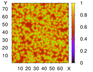
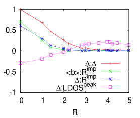
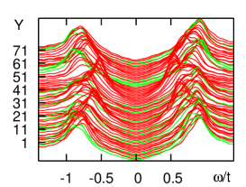
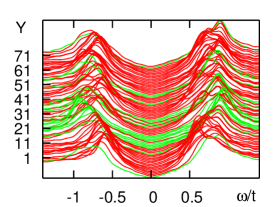
Figure 6: (Colour online) Map of the local order parameter $\Delta_{i}/t$ (upper left panel), the dependence of the correlation functions $C_{f,h}$ (upper right panel), the STM spectra taken along the vertical line at $X$=$23$ (lower left panel) and $X$=$61$ (lower right panel). The impurities are extended and influence the positions of $E^{B}_{i}$ levels changing them from the homogeneous value $0.58t$ to $0t$ in the impurity position, $0.29t$ at its nearest neighbor site, $0.425t$ and $0.5t$ at still further sites. In a similar way they also modify local energies from $V^{imp}_{i}$=$0$ to $V^{imp}_{i}$=$-0.29$ at the impurity site, $-0.145t$ at its nearest neighbor site, $-0.0775t$ and $-0.04t$ at still further sites.

The results are shown in Figure 6 for a system which, when undoped, is characterized by $E^{B}=0.58t$ and low superconducting transition temperature. The impurities are extended and modify the bosonic levels at the central and neighboring sites moving them from homogeneous value 0.58t to 0t at the impurity position, 0.29t at its nearest neighbor site, 0.425t and 0.5t at still further sites, as in Fig. 3. We assume that they also modify the local “atomic” energies from $V_{i}^{imp}=0$ to $V_{i}^{imp}=-0.29$ at the impurity, -0.145t at its nearest neighbor site, -0.0775t and -0.04t at still further sites. As a result LDOS show strong variations from point to point as can be seen in the lower panels of Figure 6.

The correlation $C_{f,h}$ between the positions of impurities and the local values of the gap is positive and around 0.4 for a small distance. Again it is lower than the correlation of the bosonic order parameter due to the on-site nature of the latter. LDOS shows strong variations from site to site which are connected with the combined effect of changes in the local values of the effective interactions and potential scattering. It is the potential scattering which suppresses sharp coherence features in the LDOS. The general observation that the peaks in LDOS are sharper at the sites with lower value of the gap remains still valid.

The map of local values of gaps shows characteristic “two shoulder” distribution with the maximum of smaller gaps centered around 0.6t and for larger gaps around 0.9t. This feature, however, is not universal and changes with the configuration and the extent of impurities.

4 Summary and conclusions

We have studied the two-component boson-fermion model in real space paying a special attention to the correlations between the local properties of the system as measured in the scanning tunnelling experiments. We have allowed the site fermion energies and bosonic levels to vary in a random fashion. Most attention has been paid to variations of the bosonic levels $E^{B}_{i}$. We propose that they are mainly affected in the process of doping of HTS parent compounds and this is a main source of inhomogeneity observed in the STM spectra.

The presence of disorder in the bosonic subsystem provides natural explanation for a number of observations on HTS. In particular, the local values of order parameters are positively correlated with the positions of impurities ($e.g.$ Figure 3). Our calculations for short ranged bosonic impurities indicate that the sharp BCS like features observed in the STM spectra might not be signatures of the well developed superconducting gap, but rather present proximity induced structures, which appear in the regions with the suppressed superconducting interactions.

In summary, our study shows the ability of the two-component boson-fermion model to describe the real space STM measurements (dependence of the differential conductance on energy, maps of the local gaps and the correlations between various parameters) with a high degree of accuracy. We limited ourselves here to the case of hard core infinitely heavy bosons. Including kinetic energy of bosons, and taking into account next nearest-neighbor fermion hopping will make the model more realistic and the results will be presented elsewhere. The model with mobile bosons has been studied in the homogeneous systems by e.g. [65, 66, 67, 68] and many other authors. This aspect seem to be important for the correct description of the phase diagram of HTS.

In this paper we focused on two - dimensional lattice and mean field theory of superconductivity. Accordingly the questions about the dimensionality and quantum fluctuation around mean field solution may arise. We consider the surface layer of the superconductor, which is coupled to the bulk. It is easy to incorporate this coupling, as well as hopping to more distant sites into our approach, but this would only slightly change the numerical results but substantially limit the size of the clusters studied.

The more important issue of quantum fluctuations [69] can in principle be addressed in a way similar to that applied recently to the inhomogeneous t-J model [70]. In the context of negative U - Hubbard model the inhomogeneities have been studied [71] by both BdG and Monte Carlo methods. The conclusion of the authors [71] is that the results of the mean - field BdG calculations agree with Monte Carlo approach which takes into account some of the fluctuations neglected by the former method. Thus we expect that our results remain qualitatively correct. Influence of the phase fluctuations for the homogeneous version of the two-component(boson-fermion) model has been addressed by some of us [41, 42] indicating the suppression of the critical temperature due to phase fluctuations. The energy gap (or ”pseudogap”) is preserved up to T*, which in the studied model roughly corresponds to $T_{c}$ obtained from the mean field BdG calculations.

References

References

- [1] T. Cren, D. Roditchev, W. Sacks, J. Klein, J.-B. Moussy, C. Deville-Cavellin, and M. Lagues, Phys. Rev. Lett. 84, 147 (2000).
- [2] S.H. Pan, J.P. O’Neal, R.L. Badzey, C. Chamon, H. Ding, J.R. Engelbrecht, Z. Wang, H. Eisaki, S. Uchida, A.K. Gupta, K.-W. Ng, E. W. Hudson, K.M. Lang, and J. C. Davis, Nature (London) 413, 282 (2001).
- [3] C. Howald, P. Fournier, and A. Kapitulnik, Phys. Rev. B 64, 100504(R) (2001).
- [4] K.M. Lang, V. Madhavan, J.E. Hoffman, E.W. Hudson, H. Eisaki, S. Uchida and J. C. Davis, Nature (London) 415, 412 (2002).
- [5] K. McElroy, J. Lee, J.A. Slezak, D.H. Lee, H. Eisaki, S. Uchida, and J.C. Davis, Science 309, 1048 (2005).
- [6] N. Doiron-Leyraud, C. Proust, D.LeBoef, J. Levalois, J.-B. Bonnemaison, R. Liang, D.A. Bonn, W.N. Hardy, and L. Taillefer, Nature (London) 447, 565 (2007).
- [7] A.F. Bangura, J.D. Fletcher, A. Carrington, J. Levallois, M. Nardone, B. Vignolle, P. J. Heard, N. Doiron-Leyraud, D. LeBoeuf, L. Taillefer, S. Adachi, C. Proust, and N. E. Hussey, Phys. Rev. Lett. 100, 047004 (2008).
- [8] S. Chakravarty, Science 319, 735 (2008).
- [9] A. Damascelli, Z. Hussain, and Z.X. Shen, Rev. Mod. Phys. 75, 473 (2003).
- [10] T.P. Devereaux and R. Hackl, Rev. Mod. Phys. 79, 175 (2007).
- [11] J.E. Sonier, Rep. Prog. Phys. 70, 1717 (2007).
- [12] D.N. Basov and T. Timusk, Rev. Mod. Phys. 77, 721 (2005).
- [13] M.R. Norman, D. Pines, and C. Kallin, Adv. Phys. 54, 715 (2005).
- [14] P.A. Lee, N. Nagaosa and X.G. Wen, Rev. Mod. Phys. 78, 17 (2006).
- [15] M. Ogata and H. Fukuyama, Rep. Prog. Phys 71, 036501 (2008).
- [16] P.A. Lee, Rep. Prog. Phys. 71, 012501 (2008).
- [17] O. Fisher, M. Kugler, I. Maggio-Aprile, and C. Berthod, Rev. Mod. Phys. 79, 353 (2007).
- [18] Ch. Renner, B. Revaz, J.Y. Genoud, and O. Fischer, J. Low Temp. Phys. 105, 1083 (1996); Ch. Renner, B. Revaz, J.Y. Genoud, K. Kadowaki, and O. Fischer, Phys. Rev. Lett. 80, 149 (1998).
- [19] A. Matsuda, T. Fujii, and T. Watanabe, Physica C 388-389, 207 (2003).
- [20] J.-X. Liu, J.-C. Wan, A.M. Goldman, Y.C. Chang, and P.Z. Jiang, Phys. Rev. Lett. 67, 2195 (1991).
- [21] A. Chang, Z.Y. Rong, Yu.M. Ivanchenko, F. Lu, and E.L. Wolf, Phys. Rev. B 46, 5692 (1992).
- [22] J.C. Davis, Acta Phys. Polon. A 104, 193 (2003).
- [23] A.V. Balatsky, I. Vekhter, and J.-X. Zhu, Rev. Mod. Phys 78, 373 (2006).
- [24] K.K. Gomes, A.N. Pasupathy, A. Pushp, S. Ono, Y. Ando, and A. Yazdani, Nature (London) 447, 569 (2007).
- [25] H. Mashima,N. Fukuo, Y. Matsumoto, G. Kinoda, T. Kondo, H. Ikuta, T. Hitosugi,and T. Hasegawa, Phys. Rev. B 73, 060502(R) (2006).
- [26] A.N. Pasupathy, A. Pushp, K.K. Gomes, C.V. Parker, J.S. Wen, Z.J. Xu, G.D. Gu, S. Ono, Y. Ando, and A. Yazdani, Science 320, 196 (2008).
- [27] J. Ranninger and S. Robaszkiewicz, Physica B 135, 468 (1985).
- [28] S. Robaszkiewicz, R. Micnas, J. Ranninger, Phys. Rev. B 36, 180 (1987).
- [29] E. Altman and A. Auerbach, Phys. Rev. B 65, 104508 (2002).
- [30] R. Micnas, J. Ranninger, and S. Robaszkiewicz, Rev. Mod. Phys 62, 113 (1990).
- [31] R. Friedberg, T.D. Lee, and H.C. Ren, Phys. Rev. B 42, 4122 (1990); R. Friedberg, T.D. Lee, and H.C. Ren, Phys. Rev. B 45, 10732 (1992).
- [32] J. Ranninger and J.M. Robin, Physica C 253, 279 (1995).
- [33] C.P. Enz, Phys. Rev. B 54, 3589 (1996).
- [34] V.B. Geshkenbein, L.B. Ioffe, and A.I. Larkin, Phys. Rev. B 55, 3173 (1997).
- [35] T. Kostyrko and J. Ranninger, Acta Phys. Polon. A 91, 399 (1997).
- [36] A.H. Castro Neto, Phys. Rev. B 64, 104509 (2001).
- [37] A. Romano, Phys. Rev. B 64, 125101 (2001).
- [38] C. Noce, Phys. Rev. B 66, 233204 (2002).
- [39] R. Micnas, B. Tobijaszewska, J. Phys.: Cond. Matt. 14, 9631 (2002).
- [40] T. Domański and J. Ranninger, Phys. Rev. B 70, 184503 (2004).
- [41] R. Micnas, S. Robaszkiewicz, and A. Bussmann-Holder, Phys. Rev B 66, 104516 (2002); J. Supercond. 17, 27 (2004).
- [42] R. Micnas, Phys. Rev. B 76, 184507 (2007).
- [43] Q. J. Chen,J. Stajic, S. Tan, and K. Levin, Phys. Reports , 412, 1 (2005). I. Bloch, J. Dalibard, W. Zwerger, Rev. Mod. Phys. 80, 885 (2008).
- [44] S. Petit and M.-B. Lepetit, EPL 80, 67005 (2009).
- [45] J. Krzyszczak, T. Domański, and K.I. Wysokiński, Acta Phys. Polon. A 114, 165 (2008);
- [46] I. Martin and A.V. Balatsky, Physica C 357-360, 46 (2001).
- [47] Q.-H. Wang, J.H. Han, D.-H. Lee, Phys. Rev B 65, 054501 (2001).
- [48] Z. Wang, J.R. Engelbrecht, S. Wang, H. Ding, and S.H. Pan, Phys. Rev. B 65, 064509 (2002).
- [49] T.S. Nunner, B.M. Andersen, A. Melikyan, and P.J. Hirschfeld, Phys. Rev. Lett. 95, 177003 (2005).
- [50] B.M. Andersen, A. Melikyan, T. S. Nunner, and P.J. Hirschfeld, Phys. Rev. B 74, 060501(R) (2006).
- [51] M.M. Maśka, Ż. Śledź, K. Czajka, and M. Mierzejewski, Phys. Rev. Lett. 99, 147006 (2007).
- [52] T. Domański and J. Ranninger, Physica C 387, 77 (2003).
- [53] A.M. Gabovich and A.I. Voitenko, Phys. Rev. B 75, 064516 (2007).
- [54] T. Domański, K.I. Wysokiński, Phys. Rev. B 66, 064517 (2002).
- [55] J.B. Ketterson and S.N. Song, Superconductivity Cambridge University Press, Cambridge (1999)
- [56] A.S. Alexandrov and N.F. Mott, Rep. Prog. Phys. 57, 1197 (1994).
- [57] T. Timusk and B. Statt, Rep. Prog. Phys. 62, 61 (1999).
- [58] G. Pawłowski and S. Robaszkiewicz, Physica A 299, 475 (2001); G. Pawłowski and S. Robaszkiewicz, Mol. Phys. Rep. 34, 76 (2001); G. Pawłowski and S. Robaszkiewicz, phys. stat. sol. (b) 236, 400 (2003); S. Robaszkiewicz and G. Pawłowski, Journ. Supercond. 17, 37 (2004); G. Pawłowski, S.Robaszkiewicz, and R.Micnas, Journ. Supercond. 17, 33 (2004); G. Pawłowski, S.Robaszkiewicz, and R.Micnas, Acta. Phys. Polon. A 106, 745 (2004); G. Pawłowski, R. Micnas, and S. Robaszkiewicz, Phys. Rev. B 81, 064514 (2010).
- [59] T. Domański, J. Ranninger, and K.I. Wysokiński, Acta Phys. Polon. B 34, 493 (2003).
- [60] K.I. Wysokiński, Phys. Rev. B 60, 16376 (1999).
- [61] For considered -wave symmetry the on-site Coulomb repulsion is not destructive.
- [62] Ż. Śledź and M. Mierzejewski, Acta Phys. Polon. A 114, 219 (2008).
- [63] A.C. Fang, L. Capriotti, D.J. Scalapino, S.A. Kivelson, N. Kaneko, M. Greven, and A. Kapitulnik, Phys. Rev. Lett. 96, 017007 (2006).
- [64] A. Ciechan, J. Krzyszczak, and K.I. Wysokiński, J. Phys. Conf. Series 150, 052283 (2009).
- [65] R. Friedberg and T.D. Lee, Phys. Rev. B 40, (1989).
- [66] N.H. Lindner and A. Auerbach, Phys. Rev. B 81, 054512 (2010).
- [67] T.A. Mamedov and M. de Llano, Phys. Rev B 75, 104506 (2007).
- [68] R. H. Squire, N.H. March, and M.L. Booth, Int. J. Quantum Chem. 109, 3516 (2009).
- [69] V.J. Emery and S.A. Kivelson, Nature 374, 434 (1995).
- [70] Y. Dubi, Y. Meir, and Y. Avishai, Nature 449, 876 (2007).
- [71] K. Aryanpour, E.R. Dagotto, M. Mayr, T. Paiva, W.E. Pickett, and R.T. Scalettar, Phys. Rev. B 73, 104518 (2006).