Exact One-Loop Evolution Invariants in the Standard Model

Abstract

Guided by considerations of flavour symmetry, we construct a set of exact Standard Model (SM) renormalisation group evolution invariants which link quark masses and mixing parameters. We examine their phenomenological implications and infer a simple combination of Yukawa coupling matrices which plays a unique role in the SM, suggesting a possible new insight into the observed spectrum of quark masses. Our evolution invariants are readily generalised to the leptons in the case of Dirac neutrinos, but do not appear to be relevant for either quarks or leptons in the MSSM.

I Introduction

Recently, there has been interest in evolution invariants Demir (2005); L.-x. Liu ; Z.-z. Xing and Luo (2010); Chang and Kuo (2002), combinations of observables which do not evolve under the renormalisation group (RG). Usually, they have been derived in various approximations, eg. assuming no fermion mixing Demir (2005), or assuming only two generations of fermions L.-x. Liu , or neglecting the contributions of light quark masses Z.-z. Xing and Luo (2010). Many work beyond the SM Demir (2005); Chang and Kuo (2002). The RG evolution equations (RGEs) of the Yukawa couplings are compactly written as matrix equations, since the problem is intrinsically flavour-symmetric - all flavours are treated equivalently. Conventional flavour observables, such as the quark and lepton masses (proportional to the eigenvalues of the Yukawa coupling matrices) or their mixing angles, break the flavour symmetry so that their RG equations are more complicated Babu (1987); Z.-z. Xing and Luo (2010). Motivated by our earlier work on flavour-symmetric variables Harrison and Scott (2005); *FCGA, we construct a set of flavour-symmetric observables whose one-loop RG equations in the SM are rather simple. These lead straightforwardly without approximation to new evolution invariants which are exact at this order. For illustration, we consider primarily the quarks, but our considerations are equally valid for the leptons in the case that neutrinos are Dirac particles, in which case more invariants follow.

We define the Hermitian squares of the Yukawa coupling matrices for charge $+\frac{2}{3}$ ($U$) and charge $-\frac{1}{3}$ ($D$) quarks respectively:

$${\cal U} =U^{\dagger}U, {\cal D} =D^{\dagger}D$$ (1)

and introduce a complete set of ten flavour-symmetric invariants (each is invariant under independent $S3$ permutations of the $(u,c,t)$ and/or the $(d,s,b)$ flavour labels):

$${\cal T}_{\scriptscriptstyle+0} =Tr({\cal U}) {\cal T}_{\scriptscriptstyle 0+} =Tr({\cal D})$$

$${\cal T}_{\scriptscriptstyle-0} =Tr({\cal U}^{-1}) {\cal T}_{\scriptscriptstyle 0-} =Tr({\cal D}^{-1})$$

$${\cal T}_{\scriptscriptstyle++} =Tr({\cal U}{\cal D}) {\cal T}_{\scriptscriptstyle+-} =Tr({\cal U}{\cal D}^{-1})$$ (2)

$${\cal T}_{\scriptscriptstyle-+} =Tr({\cal U}^{-1}{\cal D}) {\cal T}_{\scriptscriptstyle--} =Tr({\cal U}^{-1}{\cal D}^{-1})$$

$${\cal D}_{\cal U} ={\rm Det}({\cal U}) {\cal D}_{\cal D} ={\rm Det}({\cal D}).$$

The set is complete in the sense that the ten variables are fully determined by the physical masses and mixings, and are in turn, sufficient to fully determine them (up to discrete permutations of the flavour labels). A further ten analogous variables can be similarly constructed using Hermitian squares of Yukawa matrices for the neutrinos (${\cal N}$) and the charged leptons (${\cal L}$).

II SM Evolution

We start with the one-loop RG equations for the quark Yukawa coupling matrices in the SM Machacek and Vaughn (1984):

$$U^{-1}\frac{dU}{dt} =\gamma_{u}+\frac{3}{2}({\cal U}-{\cal D}),$$ (3)

$$D^{-1}\frac{dD}{dt} =\gamma_{d}+\frac{3}{2}({\cal D}-{\cal U})$$ (4)

where $t=\frac{1}{16\pi^{2}}\ln{(\mu/\mu_{0})}$ for renormalisation-scale $\mu$, and

$$\gamma_{u}=T-G_{U};\qquad\gamma_{d}=T-G_{D},$$ (5)

with:

$$T =Tr(3\,{\cal U}+3{\cal D}+{\cal N}+{\cal L}),$$ (6)

$$G_{U} =\frac{17}{12}g_{1}^{2}+\frac{9}{4}g_{2}^{2}+8g_{3}^{2},$$ (7)

$$G_{D} =\frac{5}{12}g_{1}^{2}+\frac{9}{4}g_{2}^{2}+8g_{3}^{2}$$ (8)

(the $g_{i}$ are the gauge couplings ). For ${\cal U}$ and ${\cal D}$, the Hermitian-squared matrices of Eq. (1), we get:

$$\frac{d{\cal U}}{dt} =2\gamma_{u}{\cal U}+3{\cal U}^{2}-\frac{3}{2}\{{\cal U},{\cal D}\},$$ (9)

$$\frac{d{\cal D}}{dt} =2\gamma_{d}{\cal D}+3{\cal D}^{2}-\frac{3}{2}\{{\cal U},{\cal D}\}.$$ (10)

Differentiating Eqs. (I) and using Eqs. (9) and (10), we obtain the separate evolution equations of our ten flavour-symmetric observables:

$$\frac{d{\cal T}_{\scriptscriptstyle+0}}{dt}=2\gamma_{u}{\cal T}_{\scriptscriptstyle+0}+3({\cal T}_{\scriptscriptstyle+0}^{2}-2{\cal T}_{\scriptscriptstyle-0}{\cal D}_{\cal U}-{\cal T}_{\scriptscriptstyle++})$$ (11a)

$$\frac{d{\cal T}_{\scriptscriptstyle 0+}}{dt}=2\gamma_{d}{\cal T}_{\scriptscriptstyle 0+}+3({\cal T}_{\scriptscriptstyle 0+}^{2}-2{\cal T}_{\scriptscriptstyle 0-}{\cal D}_{\cal D}-{\cal T}_{\scriptscriptstyle++})$$ (11b)

$$\frac{d{\cal T}_{\scriptscriptstyle-0}}{dt}=-2\gamma_{u}{\cal T}_{\scriptscriptstyle-0}-9+3{\cal T}_{\scriptscriptstyle-+}$$ (11c)

$$\frac{d{\cal T}_{\scriptscriptstyle 0-}}{dt}=-2\gamma_{d}{\cal T}_{\scriptscriptstyle 0-}-9+3{\cal T}_{\scriptscriptstyle+-}$$ (11d)

$$\frac{d{\cal T}_{\scriptscriptstyle++}}{dt}=2(\gamma_{u}+\gamma_{d}){\cal T}_{\scriptscriptstyle++}$$ (11e)

$$\frac{d{\cal T}_{\scriptscriptstyle--}}{dt}=-2(\gamma_{u}+\gamma_{d}){\cal T}_{\scriptscriptstyle--}$$ (11f)

$$\begin{split}&\frac{d{\cal T}_{\scriptscriptstyle+-}}{dt}=2(\gamma_{u}-\gamma_{d}+3{\cal T}_{\scriptscriptstyle+0}){\cal T}_{\scriptscriptstyle+-}-6{\cal T}_{\scriptscriptstyle+0}\\ &\text{ \qquad\quad}+6{\cal D}_{\cal U}({\cal T}_{\scriptscriptstyle--}-{\cal T}_{\scriptscriptstyle-0}{\cal T}_{\scriptscriptstyle 0-})\\ \end{split}$$ (11g)

$$\begin{split}&\frac{d{\cal T}_{\scriptscriptstyle-+}}{dt}=2(-\gamma_{u}+\gamma_{d}+3{\cal T}_{\scriptscriptstyle 0+}){\cal T}_{\scriptscriptstyle-+}-6{\cal T}_{\scriptscriptstyle 0+}\\ &\text{ \qquad\quad}+6{\cal D}_{\cal D}({\cal T}_{\scriptscriptstyle--}-{\cal T}_{\scriptscriptstyle-0}{\cal T}_{\scriptscriptstyle 0-})\\ \end{split}$$ (11h)

$$\frac{d{\cal D}_{\cal U}}{dt}=3{\cal D}_{\cal U}[2\gamma_{u}+({\cal T}_{\scriptscriptstyle+0}-{\cal T}_{\scriptscriptstyle 0+})]$$ (11i)

$$\frac{d{\cal D}_{\cal D}}{dt}=3{\cal D}_{\cal D}[2\gamma_{d}-({\cal T}_{\scriptscriptstyle+0}-{\cal T}_{\scriptscriptstyle 0+})].$$ (11j)

We make the following observations:

• Most of the variables’ evolutions have two parts:

  • a part proportional to the variable itself, whose coefficient depends at most on $\gamma_{u}$, $\gamma_{d}$, ${\cal T}_{\scriptscriptstyle+0}$ and ${\cal T}_{\scriptscriptstyle 0+}$. We call this the “pure” part.

  • a part which depends more generally on the other variables - the “mixed” part.

• The four variables ${\cal D}_{\cal U}$, ${\cal D}_{\cal D}$, ${\cal T}_{\scriptscriptstyle++}$ and ${\cal T}_{\scriptscriptstyle--}$ have only pure parts (this is also the case for Jarlskog’s determinant Jarlskog (1985); *Jarlskog2, which was the main result of Ref. Athanasiu et al. (1986)). This feature seems to be peculiar to the SM - we will rely on it in the next stage of our derivation.

III SM Evolution Invariants

Exploiting the opportunity to cancel the terms involving ${\cal T}_{\scriptscriptstyle+0}$ and ${\cal T}_{\scriptscriptstyle 0+}$ in Eqs. (11i) and (11j), we note that the quantity ${\rm Det}({\cal U}{\cal D})=({\cal D}_{\cal U}{\cal D}_{\cal D})$ has a pure evolution with exactly a factor three times the coefficient which appears in Eqs. (11e) and (11f):

$$\frac{d}{dt}\ln{{\rm Det}({\cal U}{\cal D})}=6(\gamma_{u}+\gamma_{d}).$$ (12)

We may thus form two independent combinations which are exact evolution invariants at one loop order :

$${\cal I}^{q}_{\scriptscriptstyle TD}\equiv\frac{{\cal T}_{\scriptscriptstyle++}}{({\cal D}_{\cal U}{\cal D}_{\cal D})^{\frac{1}{3}}}\equiv\frac{Tr({\cal U}{\cal D})}{{\rm Det}^{\frac{1}{3}}({\cal U}{\cal D})};\qquad\frac{d{\cal I}^{q}_{\scriptscriptstyle TD}}{dt}=0,$$ (13)

$${\cal I}^{q}_{\scriptscriptstyle PD}\equiv{\cal T}_{\scriptscriptstyle--}({\cal D}_{\cal U}{\cal D}_{\cal D})^{\frac{1}{3}}\qquad\qquad\qquad\qquad\qquad\,\,\,\,\,$$

$$\equiv Tr({\cal U}{\cal D})^{-1}{\rm Det}^{\frac{1}{3}}({\cal U}{\cal D});\qquad\frac{d{\cal I}^{q}_{\scriptscriptstyle PD}}{dt}=0.$$ (14)

The pure evolutions expressed by Eqs. (11e), (11f) and (12), and the two resulting RG invariants, Eqs. (13)-(14), are the key results of this paper. ${\cal I}^{q}_{\scriptscriptstyle TD}$ and ${\cal I}^{q}_{\scriptscriptstyle PD}$ appear to be the only exact RG invariants that can be constructed from the quark Yukawa coupling matrices alone in the SM case. We have not succeeded in finding similar exact RG invariants involving only Yukawa couplings in the MSSM or the 2 Higgs doublet model (2HDM).

We can construct entirely analogous evolution invariants using ${\cal N}$ and ${\cal L}$, the (Hermitian squares of the) Yukawa coupling matrices for the leptons (in the Dirac neutrino case). The RGEs of ${\cal N}$ and ${\cal L}$ are analogous to those in Eqs. (9)-(10) with $\gamma_{\nu}$ and $\gamma_{\ell}$ defined as in Eq. (5) with the same value of $T$ (Eq. (6)) and the gauge contributions, Eqs. (7) and (8), modifed to $G_{N}=\frac{3}{4}g_{1}^{2}+\frac{9}{4}g_{2}^{2}$ and $G_{L}=\frac{15}{4}g_{1}^{2}+\frac{9}{4}g_{2}^{2}$. The leptonic analogue of the “pure” evolution rate $2(\gamma_{u}+\gamma_{d})$, Eqs. (11e-11f) and (12), is just $2(\gamma_{\nu}+\gamma_{\ell})$, being the pure evolution rate of $Tr({\cal N}{\cal L})$ and Det${}^{\frac{1}{3}}({\cal N}{\cal L})$. Thus two more invariants follow, which we call ${\cal I}^{\ell}_{\scriptscriptstyle TD}$ and ${\cal I}^{\ell}_{\scriptscriptstyle PD}$ respectively, having definitions in terms of ${\cal N}$ and ${\cal L}$ analogous to those in Eqs. (13) and (14).

For completeness, we present here other exact one-loop evolution invariants of the SM. The $T$-dependence cancels in the ratio of any corresponding pair of purely-evolving quark and lepton observables, leaving only a dependence on gauge couplings, $g_{i}$ ($i=1..3$). The one-loop RGEs for the $g_{i}$ in the SM (at high energies) are Machacek and Vaughn (1983):

$$\frac{dg_{1}}{dt}=\frac{41}{6}g_{1}^{3},\quad\frac{dg_{2}}{dt}=-\frac{19}{6}g_{2}^{3},\quad\frac{dg_{3}}{dt}=-7g_{3}^{3}.$$ (15)

Thus eg. using Eq. (12), together with its leptonic analogue and Eq. (15), we have that:

$${\cal I}^{ql}_{\rm prod}\equiv\frac{{\rm Det}({\cal U}{\cal D})}{{\rm Det}({\cal N}{\cal L})}g_{1}^{-\frac{96}{41}}g_{3}^{-\frac{96}{7}}$$ (16)

is also an exact one-loop evolution invariant.

We note that by combining Eqs. (11i) and (11j), to form the pure-evolving ${\rm Det}({\cal U}{\cal D})$, we have effectively removed one independent evolution equation from the complete set, Eqs. (11). Thus, we may add the (independent) Jarlskog commutator Jarlskog (1985, 1985) which also has a pure RGE Athanasiu et al. (1986):

$$\frac{d}{dt}\ln({\rm Det}[{\cal U},{\cal D}])=3[2(\gamma_{u}+\gamma_{d})+Tr({\cal U})+Tr({\cal D})]$$ (17)

and likewise for the leptons. Noting the definition of $T$, Eq. (6), and using Eqs. (12), (17), their leptonic analogues, and Eq. (15), we find another RG invariant:

$${\cal I}^{ql}_{\rm comm}\equiv\frac{{\rm Det}^{3}[{\cal U},{\cal D}]{\rm Det}[{\cal N},{\cal L}]}{{\rm Det}^{3}({\cal U}{\cal D}){\rm Det}^{\frac{5}{4}}({\cal N}{\cal L})}g_{1}^{-\frac{81}{82}}g_{2}^{\frac{81}{38}}.$$ (18)

Using Eqs. (15), two more RG invariants can be constructed from gauge couplings alone:

$${\cal I}^{g}_{12} \equiv\frac{6}{41}g_{1}^{-2}+\frac{6}{19}g_{2}^{-2},$$ (19)

$${\cal I}^{g}_{13} \equiv\frac{6}{41}g_{1}^{-2}+\frac{1}{7}g_{3}^{-2}.$$ (20)

Finally, we note the SM RGE of the Higgs vacuum expectation value, $v$ Yu. F. Pirogov and Zenin (1999):

$$\frac{dv}{dt}=v\left(-T+\frac{3}{4}g_{1}^{2}+\frac{9}{4}g_{2}^{2}\right).$$ (21)

Since its product with any Yukawa coupling gives a mass term, we have that if we use mass matrices directly, rather than Yukawa matrices, the $T$- and $g_{2}$-dependences of the $\gamma_{i}$, Eq. (5), are exactly cancelled leaving only the dependences on $g_{1}$ and $g_{3}$. Thus, using $v$ together with purely-evolving quantities, and the gauge couplings, allows the construction of other RG invariants, eg.

$${\cal I}^{q}_{\scriptscriptstyle DV}\equiv{\rm Det}^{\frac{1}{3}}({\cal U}{\cal D})\,v^{4}g_{1}^{\frac{4}{41}}g_{3}^{-\frac{32}{7}}.$$ (22)

Of course, only one of these invariants involving $v$ is independent of the set already defined.

IV Evaluation

In constructing our RG invariants, we have used only four of the variables defined in Eq. (I), namely ${\cal D}_{\cal U}$, ${\cal D}_{\cal D}$, ${\cal T}_{\scriptscriptstyle++}$ and ${\cal T}_{\scriptscriptstyle--}$. While ${\rm Det}({\cal U}{\cal D})={\cal D}_{\cal U}{\cal D}_{\cal D}$ is simply the product of all six eigenvalues, variables of the form $Tr({\cal U}^{n}{\cal D}^{m})$ depend also on the mixing matrix elements. It is easy to show that such quantities are simple mass moment transforms Harrison et al. (2008) of the “$P$-matrix” Harrison et al. (2006) of transition probabilities $|V_{\alpha i}|^{2}$. Writing $u=m_{u}^{2}/v^{2}$, etc., with analogous expressions for the charge $-\frac{1}{3}$ quarks:

$$Tr({\cal U}^{n}{\cal D}^{m})$$

$$\text{\;}=\left(\begin{matrix}u^{n},&c^{n},&t^{n}\end{matrix}\right)\cdot\left(\begin{matrix}|V_{ud}|^{2}|V_{us}|^{2}|V_{ub}|^{2}\\ |V_{cd}|^{2}|V_{cs}|^{2}|V_{cb}|^{2}\\ |V_{td}|^{2}|V_{ts}|^{2}|V_{tb}|^{2}\end{matrix}\right)\cdot\left(\begin{matrix}d^{m}\\ s^{m}\\ b^{m}\end{matrix}\right)$$

$$\text{\;}=\sum_{\alpha i}m_{\alpha}^{2n}m_{i}^{2m}|V_{\alpha i}|^{2}/v^{2(m+n)}\quad\forall\,m,n,$$ (23)

(with $\alpha=u,c,t$ and $i=d,s,b$) in which terms, the flavour-symmetry property is manifest. We may now expand our new RG invariants explicitly. From Eq. (13):

$${\cal I}^{q}_{\scriptscriptstyle TD} =\sum_{\alpha i}\frac{m_{\alpha}^{2}m_{i}^{2}|V_{\alpha i}|^{2}}{(m_{u}m_{c}m_{t}m_{d}m_{s}m_{b})^{\frac{2}{3}}}$$

$$=\sum_{\alpha\neq\beta\neq\gamma,i\neq j\neq k}\left(\frac{m_{\alpha}^{2}}{m_{\beta}m_{\gamma}}\frac{m_{i}^{2}}{m_{j}m_{k}}\right)^{\frac{2}{3}}|V_{\alpha i}|^{2}.$$ (24)

From Eq. (14):

$${\cal I}^{q}_{\scriptscriptstyle PD} =(m_{u}m_{c}m_{t}m_{d}m_{s}m_{b})^{\frac{2}{3}}\sum_{\alpha i}m_{\alpha}^{-2}m_{i}^{-2}|V_{\alpha i}|^{2}$$

$$=\sum_{\alpha\neq\beta\neq\gamma,i\neq j\neq k}\left(\frac{m_{\beta}m_{\gamma}}{m_{\alpha}^{2}}\frac{m_{j}m_{k}}{m_{i}^{2}}\right)^{\frac{2}{3}}|V_{\alpha i}|^{2}.$$ (25)

Analogous formulae obtain for the leptonic RG invariants, ${\cal I}^{\ell}_{\scriptscriptstyle TD}$ and ${\cal I}^{\ell}_{\scriptscriptstyle PD}$.

From Eq. (16):

$${\cal I}^{ql}_{\rm prod}=\frac{m_{u}m_{c}m_{t}m_{d}m_{s}m_{b}}{m_{1}m_{2}m_{3}m_{e}m_{\mu}m_{\tau}}g_{1}^{-\frac{96}{41}}g_{3}^{-\frac{96}{7}},$$ (26)

while from Eq. (18):

$$\begin{split}{\cal I}^{ql}_{\rm comm}=&J_{q}^{3}f^{3}(u)f^{3}(d)\times J_{\ell}f(\nu)f(\ell)\\ &\times(y_{1}y_{2}y_{3}y_{e}y_{\mu}y_{\tau})^{-\frac{1}{4}}g_{1}^{-\frac{81}{82}}g_{2}^{\frac{81}{38}},\end{split}$$ (27)

with $f(u)=(m_{t}^{2}-m_{c}^{2})(m_{c}^{2}-m_{u}^{2})(m_{t}^{2}-m_{u}^{2})/(m_{t}^{2}m_{c}^{2}m_{u}^{2})$ and similar definitions for the charge $-\frac{1}{3}$ quarks, and the leptons. The $y_{\nu}$ and $y_{\ell}$ are the eigenvalues of ${\cal N}$ and ${\cal L}$.

For brevity, we limit the following discussion to ${\cal I}^{q}_{\scriptscriptstyle TD}$ and ${\cal I}^{q}_{\scriptscriptstyle PD}$, the RG invariants constructed only from quark Yukawa matrices. Using the experimental values of the quark masses Z.-z. Xing et al. (2008), and the Wolfenstein parameters Wolfenstein (1983), $\lambda,A,\rho$ and $\eta$ for the CKM matrix, we find both invariants to be of the order of $10^{8}$, as shown in Fig. 1, with their ratio $({\cal I}^{q}_{\scriptscriptstyle PD}/{\cal I}^{q}_{\scriptscriptstyle TD})=0.7^{+1.1}_{-0.4}$, consistent with unity.

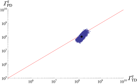
Figure 1: The black point shows the values of the RG invariants ${\cal I}^{q}_{\scriptscriptstyle TD}$ and ${\cal I}^{q}_{\scriptscriptstyle PD}$ found using quark masses from Z.-z. Xing et al. (2008) and measured values of the CKM mixings (all renormalised to $M_{Z}$). The cluster of points indicates the range allowed by experimental and theoretical uncertainties. The straight line shows the hypothesis ${\cal I}^{q}_{\scriptscriptstyle TD}={\cal I}^{q}_{\scriptscriptstyle PD}$ suggested by the data.

The strongly hierarchical quark masses and the small CKM mixing angles mean that each of them is dominated by a single leading term. We find at next-to-leading order in small quantities (small mass ratios and $\lambda^{2}$):

$${\cal I}^{q}_{\scriptscriptstyle TD}\approx\left(\frac{m_{t}}{m_{u}}\frac{m_{t}}{m_{c}}\frac{m_{b}}{m_{d}}\frac{m_{b}}{m_{s}}\right)^{\frac{2}{3}}\left(1+\lambda^{2}\left(\frac{m_{c}}{m_{t}}\frac{m_{s}}{m_{b}}\right)^{2}\right),$$ (28)

$${\cal I}^{q}_{\scriptscriptstyle PD}\approx\left(\frac{m_{t}}{m_{u}}\frac{m_{c}}{m_{u}}\frac{m_{b}}{m_{d}}\frac{m_{s}}{m_{d}}\right)^{\frac{2}{3}}(1-\lambda^{2}).$$ (29)

Since for ${\cal I}^{q}_{\scriptscriptstyle TD}$, Eq. (28), the leading term is several orders of magnitude larger than the next-to-leading term, we conclude that the combination $\left(m_{t}^{2}m_{b}^{2}/m_{u}m_{c}m_{d}m_{s}\right)^{\frac{2}{3}}$ is itself invariant to a very good approximation. At next-to-leading order, the ${\cal O}(1)$ invariant ratio is:

$$\frac{{\cal I}^{q}_{\scriptscriptstyle PD}}{{\cal I}^{q}_{\scriptscriptstyle TD}}\approx\left(m_{c}^{2}m_{s}^{2}/m_{t}m_{u}m_{b}m_{d}\right)^{\frac{2}{3}}(1-\lambda^{2}).$$ (30)

It is well-known that from the weak scale to the GUT scale, the various quark masses evolve by typically 55-65% Z.-z. Xing et al. (2008). The different mass ratios, on the other hand, vary at a slower rate, eg. $m_{b}/m_{s}$ changes by $\sim$16% and $m_{s}/m_{d}$ by $\sim$1.8%. As a check on our analysis, we have numerically solved Eqs. (3) and (4) together with the RG equations for the gauge couplings, Eq. (15), and verified that our RG invariants do not evolve at all. We have similarly verified that the leading terms of our RG invariants given in Eqs. (28) and (29) change by 0.05% or less.

V Interpretation

While the Yukawa coupling matrices ${\cal U}$ and ${\cal D}$ separately have the mixed and coupled evolutions given by Eqs. (9) and (10), it is an interesting feature, apparently peculiar to the SM, that the eigenvalues, $\lambda_{i}$, of the product matrix ${\cal U}{\cal D}$ have pure evolutions with common rate, leaving the eigenvalue ratios RG-invariant. This follows since ${\cal T}_{\scriptscriptstyle++}=Tr({\cal U}{\cal D})$ and ${\rm Det}({\cal U}{\cal D})$ with pure RGEs given in Eqs. (11e) and (12), are simply the order-one and order-three coefficients in the eigenvalue equation of the matrix ${\cal U}{\cal D}$, while ${\cal T}_{\scriptscriptstyle--}=Tr({\cal U}{\cal D})^{-1}$, with pure evolution given by Eq. (11f), is simply $P({\cal U}{\cal D})/{\rm Det}({\cal U}{\cal D})$ where:

$$P({\cal U}{\cal D})\equiv\frac{1}{2}\left[Tr^{2}({\cal U}{\cal D})-Tr({\cal U}{\cal D})^{2}\right]$$ (31)

($=\lambda_{1}\lambda_{2}+\lambda_{2}\lambda_{3}+\lambda_{3}\lambda_{1}$) is the corresponding order-two coefficient. From Eqs. (11e), (11f) and (12), we thus see that each of the coefficients in the eigenvalue equation of ${\cal U}{\cal D}$ has a pure RGE with an evolution rate which is simply given by the order of the coefficient times the same basic rate, $2(\gamma_{u}+\gamma_{d})$. Since the three eigenvalues of ${\cal U}{\cal D}$ are all order-one in terms of these coefficients via the formula for the roots of a cubic, it follows that they also have pure RGEs with common evolution rate $2(\gamma_{u}+\gamma_{d})$. We thus conclude that the ratios of the eigenvalues of ${\cal U}{\cal D}$, $\lambda_{i}/\lambda_{j}$ ($i\neq j$), are also each RG invariants (although clearly they are not individually flavour-symmetric).

In the case of a strong hierarchy, ${\cal I}^{q}_{\scriptscriptstyle TD}\approx(\lambda_{3}^{2}/\lambda_{1}\lambda_{2})^{\frac{1}{3}}$ while ${\cal I}^{q}_{\scriptscriptstyle PD}\approx(\lambda_{2}\lambda_{3}/\lambda_{1}^{2})^{\frac{1}{3}}$. These invariants could, a priori, have taken any values in nature, when, in fact, each is ${\cal O}(10^{8})$. While it is an undoubted mystery why they should be so large, it is also a puzzle why they should be so nearly equal to each other - the proximity to unity of their observed ratio, $({\cal I}^{q}_{\scriptscriptstyle PD}/{\cal I}^{q}_{\scriptscriptstyle TD})\simeq 0.7^{+1.1}_{-0.4}$ (see Fig. 1), represents a significant fine-tuning of SM parameters. Moreover, if this ratio were exactly unity, then the spectrum of the product matrix ${\cal U}{\cal D}$ would be geometric, ie.

$${\cal I}^{q}_{\scriptscriptstyle TD}={\cal I}^{q}_{\scriptscriptstyle PD}(={\cal I},~{}{\rm say})\Rightarrow\lambda_{3}/\lambda_{2}=\lambda_{2}/\lambda_{1}\approx{\cal I},$$ (32)

relations which are then valid at all scales.

It is tempting to postulate that some New Physics requires the spectrum of the matrix ${\cal U}{\cal D}$ to be exactly geometric, $({\cal I}^{q}_{\scriptscriptstyle PD}/{\cal I}^{q}_{\scriptscriptstyle TD})\equiv 1$, at some (presumably high) energy scale; the data are consistent with this hypothesis, since, as we have shown, if it is geometric at one scale, then it is geometric at all scales, as long as the one-loop RGEs of the SM remain a good approximation. It has long been known Davidson et al. (1998) that the separate spectra of the charge $+\frac{2}{3}$ and charge $-\frac{1}{3}$ quarks are approximately geometric: $m_{c}^{2}/(m_{u}m_{t})\sim{\cal O}(1)$, $m_{s}^{2}/(m_{d}m_{b})\sim{\cal O}(1)$. In contrast to our hypothesis, such separate relations are not RG-invariant and are therefore a priori less interesting and more difficult to test against data.

We consider briefly why the SM admits RG invariants constructed from only the Yukawa couplings. It can be seen from Eqs. (9) and (10), that the mixed parts of the evolution equations for the Yukawa coupling matrices ${\cal U}$ and ${\cal D}$ have balanced positive and negative coefficients. These are exploited in the evolution of the product ${\cal U}{\cal D}$ where these terms cancel on taking the trace of simple powers. The existence of balanced coefficients in the SM can be traced back to the use of the conjugate Higgs for the Yukawa couplings of the charge $\frac{2}{3}$ quarks, by contrast with the MSSM and the 2HDM, which use independent Higgs fields in each charge sector, resulting in mixed evolutions Athanasiu et al. (1986) with coefficients all having the same sign, so that no such cancellation is possible.

VI Summary

We have recast the SM RG equations using flavour-symmetric weak-basis invariant functions of the Yukawa coupling matrices, leading to the identification of exact one-loop RG invariants in the SM. We have identified two such invariants involving quark Yukawas alone, and two similar ones for leptons in the case of Dirac neutrinos. The SM seems at least somewhat unusual in allowing such RG invariants - we have not been able to find any in the MSSM or 2HDM. Despite the fact that the evolutions of ${\cal U}$ and ${\cal D}$ are coupled and mixed, the weak-basis invariants of their product matrix ${\cal U}{\cal D}$ have pure evolutions with a rate simply proportional to their order, so that its eigenvalue-ratios are RG-invariant, and are furthermore experimentally observed to be consistent with a geometric spectrum.

This work was supported by the UK Science and Technology Facilities Council (STFC). Two of us (PFH and RK) acknowledge the hospitality of the Centre for Fundamental Physics (CfFP) at the Rutherford Appleton Laboratory. We also acknowledge useful comments by Steve King and Roman Zwicky.

References

• Demir (2005) D. A. Demir, JHEP, 11, 003 (2005), arXiv:hep-ph/0408043v3 .
• (2) L.-x. Liu, arXiv:0910.1326v2[hep-ph] .
• Z.-z. Xing and Luo (2010) Z.-z. Xing and S. Luo, J. Phys. G, 37, 075018 (2010), arXiv:0912.4593v2[hep-ph] .
• Chang and Kuo (2002) S. Chang and T. K. Kuo, Phys. Rev. D, 66, 111302 (2002), arXiv:hep-ph/0205147v1 .
• Babu (1987) K. S. Babu, Z. Phys. C, 35, 69 (1987).
• Harrison and Scott (2005) P. F. Harrison and W. G. Scott, Phys. Lett. B, 628, 93 (2005), arXiv:hep-ph/0508012v2 .
• Harrison et al. (2007) P. F. Harrison, D. R. J. Roythorne,  and W. G. Scott, Phys. Lett. B, 657, 210 (2007), arXiv:0709.1439v2[hep-ph] .
• Machacek and Vaughn (1984) M. E. Machacek and M. T. Vaughn, Nucl. Phys. B, 236, 221 (1984).
• Note (1) Throughout, we use the $U(1)$ gauge coupling normalisation of Babu (1987).
• Jarlskog (1985) C. Jarlskog, Phys. Rev. Lett., 55, 1039 (1985a).
• Jarlskog (1985) C. Jarlskog, Z. Phys., C29, 491 (1985b).
• Athanasiu et al. (1986) G. G. Athanasiu, S. Dimopoulos,  and F. J. Gilman, Phys. Rev. Lett., 57, 1982 (1986).
• Note (2) Our notation for ${\cal I}^{q}_{\scriptscriptstyle TD}$ and ${\cal I}^{q}_{\scriptscriptstyle PD}$ is based on which of the coefficients of the eigenvalue equation of the matrix ${\cal U}{\cal D}$ the RG invariant may be constructed from, eg. ${\cal I}^{q}_{\scriptscriptstyle PD}=P({\cal U}{\cal D})/{\rm Det}^{\frac{2}{3}}({\cal U}{\cal D})$, where $P({\cal U}{\cal D})$ is defined in Eq. (31).
• Machacek and Vaughn (1983) M. E. Machacek and M. T. Vaughn, Nucl. Phys. B, 222, 83 (1983).
• Yu. F. Pirogov and Zenin (1999) Yu. F. Pirogov and O. V. Zenin, Eur. Phys. J. C., 10, 629 (1999), arXiv:hep-ph/9808396v1 .
• Harrison et al. (2008) P. F. Harrison, D. R. J. Roythorne,  and W. G. Scott, Proceedings of the 43rd Rencontres de Moriond on electroweak interactions and Unified Theories, La Thuile, Italy (2008), arXiv:0805.3440v1[hep-ph] .
• Harrison et al. (2006) P. F. Harrison, W. G. Scott,  and T. J. Weiler, Phys. Lett. B, 641, 372 (2006), hep-ph/0607335 .
• Z.-z. Xing et al. (2008) Z.-z. Xing, H. Zhang,  and S. Zhou, Phys. Rev. D, 77, 113016 (2008), arXiv:0712.1419v3[hep-ph] .
• Wolfenstein (1983) L. Wolfenstein, Phys. Rev. Lett., 51, 1945 (1983).
• Note (3) There is no significance to the choice of the product order ${\cal U}{\cal D}$ over ${\cal D}{\cal U}$, since the eigenvalues are the same in each case. All our results are equally applicable to both cases.
• Davidson et al. (1998) A. Davidson, T. Schwartz,  and K. C. Wali, J. Phys. G, 24, L55 (1998), hep-ph/9510444 .