Homoclinic orbits and chaos in a pair of parametrically-driven coupled nonlinear resonators

Abstract

We study the dynamics of a pair of parametrically-driven coupled nonlinear mechanical resonators of the kind that is typically encountered in applications involving microelectromechanical and nanoelectromechanical systems (MEMS & NEMS). We take advantage of the weak damping that characterizes these systems to perform a multiple-scales analysis and obtain amplitude equations, describing the slow dynamics of the system. This picture allows us to expose the existence of homoclinic orbits in the dynamics of the integrable part of the slow equations of motion. Using a version of the high-dimensional Melnikov approach, developed by Kovačič and Wiggins [Physica D, 57, 185 (1992)], we are able to obtain explicit parameter values for which these orbits persist in the full system, consisting of both Hamiltonian and non-Hamiltonian perturbations, to form so-called Šilnikov orbits, indicating a loss of integrability and the existence of chaos. Our analytical calculations of Šilnikov orbits are confirmed numerically.

I INTRODUCTION

Microelectromechanical system (MEMS) and nanoelectromechanical systems (NEMS) have been attracting much attention in recent years Roukes (2001); Cleland (2003); Craighead (2000). MEMS & NEMS resonators are typically characterized by very high frequencies, extremely small masses, and weak damping. As such, they are naturally being developed for a variety of applications such as sensing with unprecedented accuracy Rugar et al. (2004); Ilic et al. (2004); Yang et al. (2006); *Li07; *Naik09, and also for studying fundamental physics at small scales—exploring mesoscopic phenomena Schwab et al. (2000); Weig et al. (2004) and even approaching quantum behavior LaHaye et al. (2004); *Naik06; *Rocheleau10; O’Connell et al. (2010). MEMS & NEMS resonators often exhibit nonlinear behavior in their dynamics Lifshitz and Cross (2008); Rhoads et al. (2010). This includes nonlinear resonant response showing frequency pulling, multistability, and hysteresis Craighead (2000); Turner et al. (1998); Zaitsev et al. (2005); Aldridge and Cleland (2005); Kozinsky et al. (2007), as well as the formation of extended Buks and Roukes (2002) and localized Sato et al. (2006); *sato07; *sato08 collective states in arrays of coupled nonlinear resonators, and the appearance of chaotic dynamics Scheible et al. (2002); DeMartini et al. (2007); Karabalin et al. (2009). Nonlinearities are often a nuisance in actual applications, and schemes are being developed to avoid them Kacem et al. (2009); *Kacem10, but one can also benefit from the existence of nonlinearity, for example in mass-sensing applications Zhang et al. (2002); Buks and Yurke (2006), in achieving self-synchronization of large arrays Cross et al. (2004); *sync2, and even in the observation of quantum behavior Katz et al. (2007); *katz08.

MEMS & NEMS offer a wonderful experimental testing ground for theories of chaotic dynamics. Numerical investigations of a number of models of MEMS & NEMS resonators have demonstrated period-doubling transitions to chaos Liu et al. (2004); De and Aluru (2005); Park et al. (2008); Karabalin et al. (2009); Haghighi and Markazi (2010), yet there are very few analytical results. One of the simplest models of chaotic motion is that of the Duffing resonator with a double-well potential, described by the Hamiltonian

$$H(x,p)=\frac{1}{2m}p^{2}+\frac{1}{2}kx^{2}+\frac{1}{4}\alpha x^{4},$$ (1)

with $k<0$ and $\alpha>0$. This simple mechanical system has a homoclinic orbit for $H=0$, connecting a saddle at the origin of phase space to itself. Upon the addition of damping and an external drive this system develops a particular kind of chaotic motion called horseshoe chaos Wiggins (1988), which can be studied analytically using the Melnikov approach Melnikov (1963). The stable manifold leading into the saddle and the unstable manifold leading away from the saddle, which coincide in the unperturbed Hamiltonian (1), are deformed when damping and a drive are added. Yet, conditions can be found analytically using the Melnikov function, which measures the distance between the two manifolds, under which they intersect transversely leading to the possibility of observing chaotic dynamics. What one observes in practice is a random-like switching of the resonator between the two wells. Thus, having an analytical criterion for asserting the existence of chaotic motion allows one to distinguish it from random stochastic motion that might arise from noise. Such a Hamiltonian as in Eq. (1) was implemented in a MEMS device using an external electrostatic potential by DeMartini et al. DeMartini et al. (2007), and studied using the Melnikov approach.

Here we wish to study the possibility of observing horseshoe chaos in typical NEMS resonators, which are described by a potential as in Eq. (1), but of an elastic origin with $k$ and $\alpha$ both positive. Individual resonators of this type do not exhibit homoclinic orbits for any value of $H$, and therefore are not expected to display horseshoe chaos under a simple periodic drive. Nevertheless, a pair of coupled resonators of this kind—like the ones studied experimentally by Karabalin et al. Karabalin et al. (2009)—are shown below to possess homoclinic orbits in their collective dynamics, and are therefore amenable to analysis based on a high-dimensional version of the Melnikov approach Holmes and Marsden (1982); *Holmes82b. We employ here a particular method, developed by Kovačič and Wiggins Kovačič and Wiggins (1992); *kovacic2; *kovacic3, which is a combination of the high-dimensional Melnikov approach and geometric singular perturbation theory. This method enables us to find conditions, in terms of the actual physical parameters of the resonators, for the existence of an orbit in 4-dimensional phase space, which is homoclinic to a fixed point of a saddle-focus type. Such an orbit, called a Šilnikov orbit Šilnikov (1970), provides a mechanism for producing chaotic dynamics Wiggins (1988).

We study here the case of parametric, rather than direct driving, but this is not an essential requirement of our analysis. On the other hand, having weak damping, or a large quality factor, characteristic of typical MEMS & NEMS resonators, is essential for the analysis that follows. First of all, as was demonstrated in a number of earlier examples Lifshitz and Cross (2003); Bromberg et al. (2006); *kenig1; *kenig2, it leads to a clear separation of time scales—a fast scale defined by the high oscillation frequencies of the resonators, and a slow scale defined by the damping rate. This allows us to perform a multiple-scales analysis in Sec. II and obtain amplitude equations to describe the slow dynamics of the system of coupled resonators. It is in the slow dynamics that the homoclinic orbits are found. Secondly, the weak damping, which requires only a weak drive to obtain a response, allows us to treat both the damping and the drive as perturbations, even with respect to the slow dynamics. Therefore, in Sec. III we set the parametric drive amplitude and the damping to zero in the amplitude equations, which makes them integrable. This allows us, in Sec. IV, to find conditions for the existence of homoclinic orbits and to obtain analytical expressions for these orbits. We emphasize that these orbits reside in a 4-dimensional phase space, and as such are homoclinic not to a point, but rather to a whole invariant 2-dimensional manifold in the shape of a semi-infinite cylinder. Of these, we identify a subset of orbits, satisfying a particular resonance condition, that are precisely heteroclinic, connecting pairs of points in 4-dimensional phase space. In Sec. V we reintroduce the drive and the damping into the equations as small perturbations, and use the high-dimensional Melnikov method to determine which of the heteroclinic orbits, determined through the resonance condition in the unperturbed system, survives under the perturbation. In Sec. VI we study the effects of the perturbation on the dynamics within the invariant semi-infinite cylinder near the resonance condition. Finally, in Sec. VII we put everything together by calculating the parameter values for which the end-points of the unperturbed heteroclinic orbits are deformed in the perturbed system in such a way that they become connected through the dynamics on the semi-infinite cylinder, producing Šilnikov orbits, homoclinic to a fixed point of a saddle-focus type. We conclude by verifying our analytical calculation using numerical simulations. Our analysis implies that conditions exist in the coupled resonator system that could lead to chaotic motion.

II NORMAL MODE AMPLITUDE EQUATIONS

We consider a pair of resonators modeled by the equations of motion

$$\ddot{u}_{n}+u_{n} +u_{n}^{3}-\frac{1}{2}Q^{-1}(\dot{u}_{n-1}-2\dot{u}_{n}+\dot{u}_{n+1})$$

$$+\frac{1}{2}\left[D+H\cos\omega_{p}t\right](u_{n-1}-2u_{n}+u_{n+1})=0,\qquad n=1,2,$$ (2)

where $u_{n}$ describes the deviation of the $n^{th}$ resonator from its equilibrium, and we label two fictitious fixed resonators as $u_{0}=u_{3}=0$ for convenience. Detailed arguments for the choice of terms introduced into these equations of motion are discussed by Lifshitz and Cross Lifshitz and Cross (2003), who modeled the particular experimental realization of Buks and Roukes Buks and Roukes (2002), although other variations are possible Lifshitz and Cross (2008). The terms include an elastic restoring force as in Eq. (1) with positive linear and cubic contributions (whose coefficients are both scaled to 1), a dc electrostatic nearest-neighbor coupling term with a small ac component responsible for the parametric excitation (with coefficients $D$ and $H$ respectively), and a linear dissipation term, which is taken to be of a nearest neighbor form, motivated by the experimental indication Buks and Roukes (2002) that most of the dissipation comes from the electrostatic interaction between neighboring beams. Note that the electrostatic attractive force acting between neighboring beams decays with the distance between them, and thus acts to slightly soften the otherwise positive elastic restoring force. Lifshitz and Cross also considered an additional nonlinear damping term, which we neglect here for the sake of simplicity. The resonators’ quality factor $Q$ is typically high in MEMS & NEMS devices, which can be used to define a small expansion parameter $\epsilon\ll 1$, by taking $Q^{-1}=\epsilon{\hat{\gamma}}$, with $\hat{\gamma}$ of order unity. The drive amplitude is then expressed as $H=\epsilon\hat{h}$, in anticipation of the fact that parametric oscillations at half the driving frequency require a driving amplitude which is of the same order as the linear damping rate Lifshitz and Cross (2008).

Following Lifshitz and Cross (Lifshitz and Cross, 2003, Appendix B), we use multiple time scales to express the displacements of the resonators as

$$x_{1,2}(t)=\frac{\sqrt{3\epsilon}}{2}\left(A_{1}(T)e^{i\omega_{1}t}\pm A_{2}(T)e^{i\omega_{2}t}+c.c.\right)+\epsilon^{3/2}x_{1,2}^{(1)}(t)+...,$$ (3)

where $x_{1}$ is taken with the positive sign and $x_{2}$ with the negative sign; with a slow time $T=\epsilon t$, and where the normal mode frequencies are given by $\omega_{1}^{2}=1-D/2$, and $\omega_{2}^{2}=1-3D/2$. Substituting Eq. (3) into the equations of motion (II) generates secular terms that yield two coupled equations for the complex amplitudes $A_{1,2}$. If we measure the drive frequency relative to twice $\omega_{2}$ by setting $\omega_{p}=2\omega_{2}+\epsilon\Omega$, express $\omega_{1}$ relative to $\omega_{2}$ as $\omega_{1}=\omega_{2}+2\epsilon\Omega_{1}$, and express the complex amplitudes using real amplitudes and phases as

$$A_{1}(T) = a_{1}(T)e^{i[\chi_{1}(T)+(\Omega/2-2\Omega_{1})T]},$$

$$A_{2}(T) = a_{2}(T)e^{i[\chi_{2}(T)+\Omega T/2]},$$ (4)

the real and imaginary parts of the two secular amplitude equations become

$$\frac{da_{1}}{dT} = -\frac{1}{4}\hat{\gamma}a_{1}-\frac{\hat{h}}{8\omega_{1}}a_{1}\sin 2\chi_{1}-\frac{9}{8\omega_{1}}a_{2}^{2}a_{1}\sin 2(\chi_{2}-\chi_{1}),$$ (5a)

$$\frac{d\chi_{1}}{dT} = 2\Omega_{1}-\frac{1}{2}\Omega-\frac{\hat{h}}{8\omega_{1}}\cos 2\chi_{1}+\frac{9}{8\omega_{1}}\bigl{[}a_{1}^{2}+2a_{2}^{2}+a_{2}^{2}\cos 2(\chi_{2}-\chi_{1})\bigr{]},$$ (5b)

$$\frac{da_{2}}{dT} = -\frac{3}{4}\hat{\gamma}a_{2}-\frac{3\hat{h}}{8\omega_{2}}a_{2}\sin 2\chi_{2}-\frac{9}{8\omega_{2}}a_{1}^{2}a_{2}\sin 2(\chi_{1}-\chi_{2}),$$ (5c)

$$\frac{d\chi_{2}}{dT} = -\frac{1}{2}\Omega-\frac{3\hat{h}}{8\omega_{2}}\cos 2\chi_{2}+\frac{9}{8\omega_{2}}\bigl{[}a_{2}^{2}+2a_{1}^{2}+a_{1}^{2}\cos 2(\chi_{1}-\chi_{2})\bigr{]}.$$ (5d)

Steady-state solutions, oscillating at half the parametric drive frequency, are obtained by setting $da_{i}/dT=d\chi_{i}/dT=0$ in Eqs. (5) and solving the resulting algebraic equations. We are interested in extending the investigation of these amplitude equations. In particular, we want to identify the conditions under which they may display chaotic dynamics. We should note that equations similar to (5) were also used for modeling a variety of parametrically driven two-degree of freedom systems such as surface waves in nearly-square tanks or vibrations of nearly-square thin plates or of beams with nearly-square cross sections Meron and Procaccia (1986); *meron862; Feng and Sethna (1989); *feng931; *fandw; *feng95; Zhang (2001); Moehlis et al. (2009).

III UNPERTURBED EQUATIONS—SETTING DAMPING AND DRIVE TO ZERO

We first consider the integrable parts of Eqs. (5), obtained by setting $\hat{\gamma}=\hat{h}=0$, which after a rescaling of the amplitudes, $a_{1}\rightarrow a_{1}\sqrt{\omega_{2}8/9}$, and $a_{2}\rightarrow a_{2}\sqrt{\omega_{1}8/9}$, become

$$\frac{da_{1}}{dT} = a_{2}^{2}a_{1}\sin 2(\chi_{1}-\chi_{2}),$$ (6a)

$$\frac{d\chi_{1}}{dT} = -\left(\frac{\Omega}{2}-2\Omega_{1}\right)+a_{2}^{2}\left[2+\cos 2(\chi_{1}-\chi_{2})\right]+\frac{\omega_{2}}{\omega_{1}}a_{1}^{2},$$ (6b)

$$\frac{da_{2}}{dT} = -a_{1}^{2}a_{2}\sin 2(\chi_{1}-\chi_{2}),$$ (6c)

$$\frac{d\chi_{2}}{dT} = -\frac{\Omega}{2}+a_{1}^{2}\left[2+\cos 2(\chi_{1}-\chi_{2})\right]+\frac{\omega_{1}}{\omega_{2}}a_{2}^{2}.$$ (6d)

In Sec. V we will reintroduce the driving and damping terms as a perturbation. We transform Eqs. (6) into a more familiar form, which has been studied in the context of higher dimensional Melnikov methods Wiggins (1988); Kovačič and Wiggins (1992); Kovačič (1995), by changing to two pairs of action-angle variables: (i) $B=a_{1}^{2}/2$, $\theta=\chi_{1}-\chi_{2}$; and (ii) $I=(a_{1}^{2}+a_{2}^{2})/2$, $\phi=\chi_{2}$. After defining $\delta=\omega_{1}/\omega_{2}$, and rescaling time as $T\rightarrow T/2$, we obtain the unperturbed Hamilton equations

$$\frac{dB}{dT} = -\frac{\partial\tilde{H}_{0}(B,\theta,I)}{\partial\theta}=2B(I-B)\sin 2\theta,$$ (7a)

$$\frac{d\theta}{dT} = \frac{\partial\tilde{H}_{0}(B,\theta,I)}{\partial B}=\Omega_{1}+I(2-\delta+\cos 2\theta)-B\left(4-\frac{\delta^{2}+1}{\delta}+2\cos 2\theta\right),$$ (7b)

$$\frac{dI}{dT} = -\frac{\partial\tilde{H}_{0}(B,\theta,I)}{\partial\phi}=0,$$ (7c)

$$\frac{d\phi}{dT} = \frac{\partial\tilde{H}_{0}(B,\theta,I)}{\partial I}=\delta I-\frac{\Omega}{4}+B(2-\delta+\cos 2\theta),$$ (7d)

where the Hamiltonian $\tilde{H}_{0}$, which generates these equations, is expressed as

$$\tilde{H}_{0}(B,\theta,I)=\frac{\delta I^{2}}{2}-\frac{\Omega}{4}I-B^{2}\left(2-\frac{\delta^{2}+1}{2\delta}\right)+B\left[I(2-\delta)+\Omega_{1}\right]+B(I-B)\cos 2\theta.$$ (8)

Thus, both $I$ and $\tilde{H}_{0}$ are constants of the motion in the unperturbed system. Note that $(B,\theta,I,\phi)\in\mathbb{R}^{+}\times\mathbb{S}\times\mathbb{R}^{+}\times\mathbb{S}$, where $\mathbb{S}$ is the unit circle, and $\mathbb{R}^{+}$ are the non-negative reals.

It is convenient to describe the dynamics also in terms of the Cartesian variables $x=a_{1}\cos(\chi_{1}-\chi_{2})=\sqrt{2B}\cos\theta$ and $y=a_{1}\sin(\chi_{1}-\chi_{2})=\sqrt{2B}\sin\theta$, in place of $B$ and $\theta$, thereby obtaining the Hamilton equations

$$\frac{dx}{dT} = -\frac{\partial H_{0}(x,y,I)}{\partial y}=y^{3}\left(1-\frac{\delta^{2}+1}{2\delta}\right)+x^{2}y\left(2-\frac{\delta^{2}+1}{2\delta}\right)-y\left[I(1-\delta)+\Omega_{1}\right],$$ (9a)

$$\frac{dy}{dT} = \frac{\partial H_{0}(x,y,I)}{\partial x}=-x^{3}\left(3-\frac{\delta^{2}+1}{2\delta}\right)-y^{2}x\left(2-\frac{\delta^{2}+1}{2\delta}\right)+x\left[I(3-\delta)+\Omega_{1}\right],$$ (9b)

$$\frac{dI}{dT} = -\frac{\partial H_{0}(x,y,I)}{\partial\phi}=0,$$ (9c)

$$\frac{d\phi}{dT} = \frac{\partial H_{0}(x,y,I)}{\partial I}=\delta I-\frac{\Omega}{4}+\frac{x^{2}}{2}(3-\delta)+\frac{y^{2}}{2}(1-\delta),$$ (9d)

where $y$ plays the role of a coordinate and $x$ is its conjugate momentum, and where the Hamiltonian $H_{0}$ is now given by

$$H_{0}(x,y,I) = \frac{\delta I^{2}}{2}-\frac{\Omega}{4}I-\frac{x^{4}}{4}\left(3-\frac{\delta^{2}+1}{2\delta}\right)-\frac{y^{4}}{4}\left(1-\frac{\delta^{2}+1}{2\delta}\right)-x^{2}y^{2}\left(1-\frac{\delta^{2}+1}{4\delta}\right)$$ (10)

$$+ \frac{x^{2}}{2}\left[I(3-\delta)+\Omega_{1}\right]+\frac{y^{2}}{2}\left[I(1-\delta)+\Omega_{1}\right].$$

IV ANALYTICAL EXPRESSIONS FOR HOMOCLINIC ORBITS

We wish to identify the conditions under which there exist homoclinic orbits in the unperturbed system. These orbits will potentially lead to chaotic dynamics once we reintroduce the damping and the drive in the form of small perturbations. We therefore consider the fixed point $x=y=0$ in the unperturbed $(x,y)$ plane, as given by Eqs. (9a) and (9b). A linear analysis of this fixed point reveals that it is a saddle for values of the positive constant of motion $I$, that satisfy the inequality $[I(1-\delta)+\Omega_{1}][I(3-\delta)+\Omega_{1}]<0$. This implies that the fixed point at $x=y=0$ is never a saddle if the fixed parameter $\delta<1$; it is a saddle for $1<\delta<3$, if $I>\Omega_{1}/(\delta-1)$; and it is a saddle for $\delta>3$, if $\Omega_{1}/(\delta-1)<I<\Omega_{1}/(\delta-3)$. We shall restrict ourselves here to values $1<\delta<3$, therefore to obtain a saddle one must only ensure that $I>\Omega_{1}/(\delta-1)$. In the full four-dimensional system given by Eqs. (9) this saddle point describes a two-dimensional invariant semi-infinite cylinder, or annulus,

$$\mathscr{M}=\left\{(x,y,I,\phi)\ \big{|}\ x=0,\ y=0,\ \frac{\Omega_{1}}{\delta-1}<I\right\},\qquad 1<\delta<3,$$ (11)

where $\phi$ is unrestricted within the unit circle. The trajectories on $\mathscr{M}$ are periodic orbits given by $I=\textmd{constant}$ and $\phi=(\delta I-\Omega/4)T+\phi_{0}$. For the resonant value of $I\equiv I^{r}=\Omega/4\delta$ the rotation frequency vanishes, and the periodic orbit becomes a circle of fixed points. Of course, this trivial unperturbed dynamics on $\mathscr{M}$ undergoes a dramatic change under the addition of perturbations.

The two-dimensional invariant annulus $\mathscr{M}$ has three-dimensional stable and unstable manifolds, denoted as $W^{s}(\mathscr{M})$ and $W^{u}(\mathscr{M})$, respectively, which coincide to form a three-dimensional homoclinic manifold $\Gamma\equiv W^{s}(\mathscr{M})\cap W^{u}(\mathscr{M})$. Trajectories on the homoclinic manifold $\Gamma$ are homoclinic orbits that connect the origin of the $(x,y)$ plane to itself. Thus, the constant value of the Hamiltonian along such an orbit is equal to its value at the origin, namely $H_{0}(0,0,I)=H_{0}(x,y,I)=\tilde{H}_{0}(B,\theta,I)$, which immediately yields an equation for the homoclinic orbits in terms of the action-angle variables

$$B^{h}(\theta,I)=\frac{2\delta\left[I\left(\delta-2-\cos 2\theta\right)-\Omega_{1}\right]}{\delta^{2}-2\delta\left(2+\cos 2\theta\right)+1}.$$ (12)

To obtain the temporal dependence of the dynamical variables along the homoclinic orbit, we substitute the homoclinic orbit equation (12) into Eq. (7b), to get

$$\frac{d\theta}{dT}=I(\delta-2-\cos 2\theta)-\Omega_{1}.$$ (13)

Next, we note that $\chi_{1}=\phi+\theta$, and use the Hamiltonian (8) to get

$$\frac{d\chi_{1}}{dT}=I\delta-\frac{\Omega}{4}+B\frac{1-\delta^{2}}{2\delta}.$$ (14)

We then integrate Eq. (13), substitute the result into Eq. (12), and the latter into Eq. (14), and finally integrate Eq. (14) to obtain analytical expressions for the temporal dependence of the dynamical variables along orbits that are homoclinic to $\mathscr{M}$.

For $I>2\delta\Omega_{1}/(\delta^{2}-1)$ we define $q\equiv I(\delta^{2}-1)-2\delta\Omega_{1}>0$, and find that $\theta_{0}\equiv\theta(T=0)=0,\pi$, and that the homoclinic orbits are given by

$$B^{h}(T,I) = \frac{2\delta a^{2}}{q\cosh(2aT)+p},$$ (15a)

$$\tan\left(\theta^{h}(T,I)\right) = -\sqrt{\frac{I(\delta-3)-\Omega_{1}}{I(1-\delta)+\Omega_{1}}}\tanh(aT),$$ (15b)

$$\chi_{1}^{h}(T,I) = -\frac{a(\delta^{2}-1)}{\sqrt{p^{2}-q^{2}}}\text{ arctanh}\left(\sqrt{\frac{p-q}{p+q}}\tanh aT\right)+(\delta I-\frac{\Omega}{4})T+\chi_{1}(0),$$ (15c)

$$\phi^{h}(T,I) = \chi_{1}^{h}(T,I)-\theta^{h}(T,I),$$ (15d)

where

$$p = \Omega_{1}(\delta^{2}-4\delta+1)-I(\delta^{3}-6\delta^{2}+7\delta-2),$$

$$a^{2} = -\Omega_{1}^{2}+2I\Omega_{1}(\delta-2)-I^{2}(\delta-3)(\delta-1).$$ (16)

For $I<2\delta\Omega_{1}/(\delta^{2}-1)$ we redefine $q\equiv 2\delta\Omega_{1}-I(\delta^{2}-1)>0$, and find that $\theta_{0}=\pm\pi/2$, and that the homoclinic orbits are given by Eqs. (15), with Eq. (15b) replaced by

$$\cot\left(\theta^{h}(T,I)\right)=-\sqrt{\frac{I(1-\delta)+\Omega_{1}}{I(\delta-3)-\Omega_{1}}}\tanh(aT).$$ (17)

Thus, exactly at $I=2\delta\Omega_{1}/(\delta^{2}-1)$ (or $q=0$) there is a global bifurcation in which the homoclinic orbit rotates through an angle of $\pi/2$.

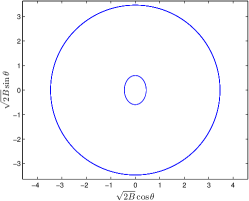
(a) $\ I=6$

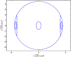
(b) $\ I=10$

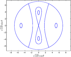
(c) $\ I=25$

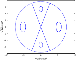
(d) $\ I=28.4267$

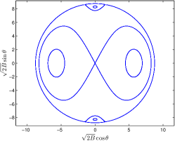
(e) $\ I=38.5$

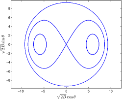
(f) $\ I=43$

Figure 1: Numerical phase portraits of the unperturbed $(x,y)$ plane for $\delta=2$, $\Omega_{1}=21.32$, and different values of $I$ as noted in the individual captions. All figures show the trajectories for which $B$ has a fixed value equal to $I$. As explained in the text and for $\delta=2$, four hyperbolic fixed points appear on the $B=I$ circle for $2\Omega_{1}/5=8.528<I<2\Omega_{1}=42.64$; the $B=0$ fixed point changes from a center to a saddle at $I=\Omega_{1}=21.32$; and a global bifurcation rotating the homoclinic orbit through an angle of $\pi/2$, shown in panel (d), occurs at $I=4\Omega_{1}/3\simeq 28.4267$.

Some of the phase-space portraits of the unperturbed $(x,y)$ plane are calculated numerically from Eqs. (7a) and (7b), for different values of $I$, and shown in Fig. 1. From Eq. (7a) it follows that the value of $B$ is fixed if (a) $B=0$; or (b) $B=I$; or (c) $\theta$ is an integer multiple of $\pi/2$ and $\theta$ is fixed. Figures 1(a)–(f) all show the trajectories for which $B$ has a fixed value equal to $I$. Four hyperbolic fixed points appear on the $B=I$ circle for $\Omega_{1}/(3-1/\delta)\leq I\leq\Omega_{1}(1-1/\delta)$, where solutions exist to the equation $\partial\theta/\partial T=0$ with $B$ replaced by $I$ [Figs. 1(b)–(e)]. As expected, the origin $B=0$ is always a fixed point—a center for small values of $I$ [Figs. 1(a),(b)], which undergoes a pitchfork bifurcation into a saddle when $\partial\theta/\partial T=0$ with $B=0$, occurring at $I=\Omega_{1}/(\delta-1)$ [Figs. 1(c)–(f)]. Additional centers appear whenever $\theta$ is an integer multiple of $\pi/2$ and solutions exist to the equation $\partial\theta/\partial T=0$ with $\cos 2\theta=\pm 1$ [Figs. 1(b)–(f)]. The global bifurcation at $I=2\Omega_{1}\delta/(\delta^{2}-1)$ where the homoclinic orbit rotates by $\pi/2$ is shown in Fig. 1(d).

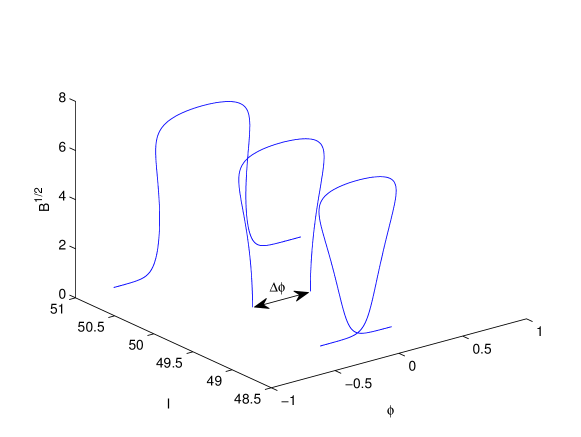
Figure 2: Orbits homoclinic to $\mathscr{M}$. For $I=I^{r}$ (the orbit in the middle), $d\phi/dT=0$ on $\mathscr{M}$, and the orbit is heteroclinic, connecting fixed points on $\mathscr{M}$ that are $\Delta\phi$ apart. For $I\lessgtr I^{r}$, $d\phi/dT\lessgtr 0$ on $\mathscr{M}$. The parameters are $\delta=2,\Omega=400,\Omega_{1}=21.32$.

Note that we refer to the orbits given by Eqs. (15) as homoclinic since they are homoclinic to $\mathscr{M}$. A few of these orbits are shown in Fig. 2. At resonance, for $I=I^{r}$, the orbits are truly heteroclinic, connecting fixed points that are $\Delta\phi$ apart, where $\Delta\phi=\Delta\chi_{1}-\Delta\theta$, and

$$\Delta\theta = -2\textmd{arctan}\sqrt{\frac{I^{r}(\delta-3)-\Omega_{1}}{I^{r}(1-\delta)+\Omega_{1}}},$$ (18a)

$$\Delta\chi_{1} = -\frac{2a(\delta^{2}-1)}{\sqrt{p^{2}-q^{2}}}\textmd{arctanh}\sqrt{\frac{p-q}{p+q}},$$ (18b)

and where for any variable $f$, $\Delta f\equiv f(T=\infty)-f(T=-\infty)$. Such an unperturbed heteroclinic orbit is shown in the middle of Fig. 2.

Figure 3: Results of a numerical integration of Eqs. (5) for different values of the initial amplitude of the second mode $a_{2}(0)$, with $\hat{h}=\hat{\gamma}=0$, $\omega_{1}=0.8528$, $\omega_{2}=\omega_{1}/2$, $\Omega_{1}=21.32$, and $\Omega=400$. As expected, for $a_{2}(0)>\sqrt{16\Omega_{1}\omega_{1}\omega_{2}/9(\omega_{1}-\omega_{2})}\simeq 5.68$ the origin becomes a saddle, which rotates through an angle of $\pi/2$ at $a_{2}(0)=\sqrt{32\Omega_{1}\omega_{1}^{2}\omega_{2}/9(\omega_{1}^{2}-\omega_{2}^{2})}\simeq 6.46$.

We wish to demonstrate the results obtained so far also in terms of original amplitude equations (5) with $\hat{h}=\hat{\gamma}=0$. The point $x=y=0$ corresponds to $a_{1}=0$ in Eqs. (5). To start the simulation near this point, we initiate the numerical solution with $a_{1}(0)\ll 1$, which through the definition of $I$ implies that $a_{2}(0)\simeq\sqrt{16I\omega_{1}/9}$. The condition for having a saddle at the origin of Eqs. (9a) and (9b), $I>\Omega_{1}/(\delta-1)$, translates into the condition $a_{2}(0)>\sqrt{16\Omega_{1}\omega_{1}/9(\delta-1)}=\sqrt{16\Omega_{1}\omega_{1}\omega_{2}/9(\omega_{1}-\omega_{2})}$. The condition for the global bifurcation, rotating the homoclinic orbit through $\pi/2$, given by $I=2\delta\Omega_{1}/(\delta^{2}-1)$, translates into $a_{2}(0)=\sqrt{32\Omega_{1}\omega_{1}^{2}\omega_{2}/9(\omega_{1}^{2}-\omega_{2}^{2})}$. These conditions are verified by a numerical integration of Eqs. (5) by varying the initial amplitude of the out-of-phase mode, $a_{2}(0)$, as shown in Fig. 3.

V HOMOCLINIC INTERSECTIONS IN THE PERTURBED SYSTEM

After having calculated the homoclinic orbits in the unperturbed system, we now reintroduce the drive and the damping as perturbations and study how they affect the dynamics. In particular, we want to study the nature of the invariant annulus $\mathscr{M}$, and its stable and unstable manifolds, $W^{s}(\mathscr{M})$ and $W^{u}(\mathscr{M})$, under the perturbation, and use the Melnikov criterion to find the conditions under which they can still intersect. The perturbed equations are written in terms of the action-angle variables as

$$\frac{dB}{dT} = 2B(I-B)\sin 2\theta-\xi hB\sin 2(\phi+\theta)-\xi\gamma B,$$ (19a)

$$\frac{d\theta}{dT} = \Omega_{1}+I(2-\delta+\cos 2\theta)-B\left(4-\frac{\delta^{2}+1}{\delta}+2\cos 2\theta\right)$$ (19b)

$$- \frac{\xi h}{2}\left[\cos 2(\phi+\theta)-3\delta\cos 2\phi\right],$$

$$\frac{dI}{dT} = -\xi h\left[3\delta(I-B)\sin 2\phi+B\sin 2(\phi+\theta)\right]-\xi\gamma(3I-2B),$$ (19c)

$$\frac{d\phi}{dT} = -\frac{\Omega}{4}+\delta I+B(2-\delta+\cos 2\theta)-\frac{3\xi h\delta}{2}\cos(2\phi),$$ (19d)

where we have quantified the perturbations by expressing the drive amplitude and the damping as $\hat{h}=\xi 8\omega_{1}h$ and $\hat{\gamma}=\xi 4\gamma$, respectively, where $\xi\ll 1$ is a small parameter. It is instructive to write the perturbed system in the general form

$$\frac{dB}{dT} = -\frac{\partial\tilde{H}_{0}(B,\theta,I)}{\partial\theta}+\xi g^{B}=-\frac{\partial\tilde{H}_{0}(B,\theta,I)}{\partial\theta}+\xi\left(-\frac{\partial\tilde{H}_{1}(B,\theta,I,\phi)}{\partial\theta}+d^{B}\right),$$ (20a)

$$\frac{d\theta}{dT} = \frac{\partial\tilde{H}_{0}(B,\theta,I)}{\partial B}+\xi g^{\theta}=\frac{\partial\tilde{H}_{0}(B,\theta,I)}{\partial B}+\xi\frac{\partial\tilde{H}_{1}(B,\theta,I,\phi)}{\partial B},$$ (20b)

$$\frac{dI}{dT} = \xi g^{I}=\xi\left(-\frac{\partial\tilde{H}_{1}(B,\theta,I,\phi)}{\partial\phi}+d^{I}\right),$$ (20c)

$$\frac{d\phi}{dT} = \frac{\partial\tilde{H}_{0}(B,\theta,I)}{\partial I}+\xi g^{\phi}=\frac{\partial\tilde{H}_{0}(B,\theta,I)}{\partial I}+\xi\frac{\partial\tilde{H}_{1}(B,\theta,I,\phi)}{\partial I},$$ (20d)

where the perturbations due to the parametric drive are generated from the Hamiltonian

$$\tilde{H}_{1}(B,\theta,I,\phi)=-\frac{h}{2}\left[B\cos 2(\phi+\theta)+3\delta(I-B)\cos 2\phi\right],$$ (21)

and the dissipative perturbations are given by $d^{B}=-\gamma B$ and $d^{I}=-\gamma(3I-2B)$. Similarly, in terms of the Cartesian variables, the perturbed system is written in this general form as

$$\frac{dx}{dT} = -\frac{\partial H_{0}(x,y,I)}{\partial y}+\xi g^{x}=-\frac{\partial H_{0}(x,y,I)}{\partial y}+\xi\left(-\frac{\partial H_{1}(x,y,I,\phi)}{\partial y}+d^{x}\right),$$ (22a)

$$\frac{dy}{dT} = \frac{\partial H_{0}(x,y,I)}{\partial x}+\xi g^{y}=\frac{\partial H_{0}(x,y,I)}{\partial x}+\xi\left(\frac{\partial H_{1}(x,y,I,\phi)}{\partial x}+d^{y}\right),$$ (22b)

$$\frac{dI}{dT} = \xi g^{I}=\xi\left(-\frac{\partial H_{1}(x,y,I,\phi)}{\partial\phi}+d^{I}\right),$$ (22c)

$$\frac{d\phi}{dT} = \frac{\partial H_{0}(x,y,I)}{\partial I}+\xi g^{\phi}=\frac{\partial H_{0}(x,y,I)}{\partial I}+\xi\frac{\partial H_{1}(x,y,I,\phi)}{\partial I},$$ (22d)

with

$$H_{1}(x,y,I,\phi)=\frac{h}{4}\left\{\left[\left(3\delta-1\right)x^{2}+\left(3\delta+1\right)y^{2}-6\delta I\right]\cos 2\phi+2xy\sin 2\phi\right\},$$ (23)

and where $d^{x}=-\gamma x/2$, $d^{y}=-\gamma y/2$, and $d^{I}=-\gamma(3I-x^{2}-y^{2})$.

For $0<\xi\ll 1$ the unperturbed invariant annulus $\mathscr{M}$, and its stable and unstable manifolds, $W^{s}(\mathscr{M})$ and $W^{u}(\mathscr{M})$, persist as a locally invariant annulus $\mathscr{M}_{\xi}$ with stable and unstable manifolds, $W^{s}(\mathscr{M}_{\xi})$ and $W^{u}(\mathscr{M}_{\xi})$ Wiggins (1988); Kovačič and Wiggins (1992); Kovačič (1992, 1995); Kaper and Kovačič (1996); Feng and Sethna (1993). Due to the fact that we use parametric rather than direct excitation, the point $x=y=0$ remains a fixed point of the perturbed Eq. (22a) and (22b), so $\mathscr{M}_{\xi}$ is defined just like $\mathscr{M}$ in Eq. (11). However, the term locally invariant means that trajectories with initial conditions on $\mathscr{M}_{\xi}$ may leave it through its lower boundary at $I=\Omega_{1}/(\delta-1)$. We want to find intersections of the manifolds $W^{s}(\mathscr{M}_{\xi})$ and $W^{u}(\mathscr{M}_{\xi})$, because such intersections may contain orbits that are homoclinic to $\mathscr{M}_{\xi}$. This is done by calculating the Melnikov integral, $M(I,\phi_{0})$, which is a measure of the distance between these manifolds. If the Melnikov integral has simple zeros [$M(I,\phi_{0})=0$ and $\partial M(I,\phi_{0})/\partial\phi_{0}\neq 0$], the three-dimensional manifolds $W^{s}(\mathscr{M}_{\xi})$ and $W^{u}(\mathscr{M}_{\xi})$ intersect transversely along two-dimensional surfaces.

The Melnikov integral is given by Wiggins (1988); Kovačič and Wiggins (1992); Kovačič (1992, 1995)

$$M(I,\phi_{0})=\int_{-\infty}^{\infty}\langle\textbf{n}(x^{h},y^{h},I),\textbf{g}(x^{h},y^{h},I,\phi^{h}+\phi_{0})\rangle dT,$$ (24)

where

$$\textbf{n}(x,y,I)=\bigg{(}\frac{\partial H_{0}(x,y,I)}{\partial x},\frac{\partial H_{0}(x,y,I)}{\partial y},\frac{\partial H_{0}(x,y,I)}{\partial I}-\frac{\partial H_{0}(0,0,I)}{\partial I}\bigg{)},$$ (25)

$$\textbf{g}(x,y,I,\phi)=\left(g^{x},g^{y},g^{I}\right),$$ (26)

$x^{h}(T,I)$, $y^{h}(T,I)$, and $\phi^{h}(T,I)$ are the homoclinic orbits given by Eqs. (15), and angular brackets denote the standard inner product. At resonance, the Melnikov integral $M(I^{r},\phi_{0})$ can be calculated explicitly, because then $\partial H_{0}(0,0,I^{r})/\partial I=0$ and the integrand of the Melnikov integral is given by

$$\langle\textbf{n},\textbf{g}\rangle = \frac{\partial H_{0}}{\partial x}g^{x}+\frac{\partial H_{0}}{\partial y}g^{y}+\frac{\partial H_{0}}{\partial I}g^{I}$$ (27)

$$= -\frac{\partial H_{0}}{\partial x}\frac{\partial H_{1}}{\partial y}+\frac{\partial H_{0}}{\partial y}\frac{\partial H_{1}}{\partial x}-\frac{\partial H_{0}}{\partial I}\frac{\partial H_{1}}{\partial\phi}+\frac{\partial H_{0}}{\partial x}d^{x}+\frac{\partial H_{0}}{\partial y}d^{y}+\frac{\partial H_{0}}{\partial I}d^{I}.$$

For the unperturbed orbits we can use the chain rule and the fact that $dI/dT=0$ to obtain the relation

$$\frac{dH_{1}}{dT}=\frac{\partial H_{0}}{\partial x}\frac{\partial H_{1}}{\partial y}-\frac{\partial H_{0}}{\partial y}\frac{\partial H_{1}}{\partial x}+\frac{\partial H_{0}}{\partial I}\frac{\partial H_{1}}{\partial\phi},$$ (28)

so the Melnikov integrand reduces to

$$\langle\textbf{n},\textbf{g}\rangle=-\frac{dH_{1}}{dT}+\frac{\partial H_{0}}{\partial x}d^{x}+\frac{\partial H_{0}}{\partial y}d^{y}+\frac{\partial H_{0}}{\partial I}d^{I}.$$ (29)

Upon transforming to the action-angle variables one has

$$\frac{\partial H_{0}}{\partial x}d^{x}+\frac{\partial H_{0}}{\partial y}d^{y}=\frac{\partial\tilde{H}_{0}}{\partial B}d^{B},$$ (30)

and so the integrand (29) becomes

$$\langle\textbf{n},\textbf{g}\rangle = -\frac{d\tilde{H}_{1}}{dT}+\frac{\partial\tilde{H}_{0}}{\partial B}d^{B}+\frac{\partial\tilde{H}_{0}}{\partial I}d^{I}=-\frac{d\tilde{H}_{1}}{dT}-\gamma B\frac{d\theta}{dT}-\gamma(3I^{r}-2B)\frac{d\phi}{dT}$$ (31)

$$= -\frac{d\tilde{H}_{1}}{dT}-3\gamma I^{r}\frac{d\phi}{dT}+2\gamma B\frac{d\chi_{1}}{dT}-3\gamma B\frac{d\theta}{dT},$$

where we recall that $\chi_{1}=\theta+\phi$.

We can now explicitly integrate each of the terms in the integrand (31). From Eq. (21), owing to the fact that on the homoclinic orbits $B(\pm\infty)=0$, the first of these yields

$$\int^{\infty}_{-\infty}\frac{d\tilde{H}_{1}}{dT}dT = -\frac{3\delta I^{r}h}{2}\left[\cos 2\phi(\infty)-\cos 2\phi(-\infty)\right]$$ (32)

$$= -\frac{3\delta I^{r}h}{2}\left[\cos 2(\phi_{0}+\Delta\phi/2)-\cos 2(\phi_{0}-\Delta\phi/2)\right]$$

$$= 3\delta I^{r}h\sin 2\phi_{0}\sin\Delta\phi,$$

where we recall that $\Delta\phi=\phi(\infty)-\phi(-\infty)$. The second term in (31) immediately yields $-3\gamma I^{r}\Delta\phi$. For the third term in (31) we use Eq. (14), which on resonance yields

$$\int^{\infty}_{-\infty}B\frac{d\chi_{1}}{dT}dT = \frac{1-\delta^{2}}{2\delta}\int^{\infty}_{-\infty}B^{2}dT$$ (33)

$$= (1-\delta^{2})2\delta a^{3}\left(\frac{2p}{(p^{2}-q^{2})^{3/2}}\textmd{ arctanh}\sqrt{\frac{p-q}{p+q}}+\frac{1}{q^{2}-p^{2}}\right)\equiv\Delta\sigma.$$

For the fourth and last term in (31) we use Eq. (12) and get

$$\int Bd\theta=I^{r}\theta+\frac{I^{r}(\delta^{2}-1)-2\delta\Omega_{1}}{(\delta-1)\sqrt{\delta^{2}-6\delta+1}}\arctan\left(\frac{\delta-1}{\sqrt{\delta^{2}-6\delta+1}}\tan\theta\right),$$ (34)

and after substituting the limits, using Eq. (15b), we get

$$\int Bd\theta = I^{r}\Delta\theta-2\frac{I^{r}(\delta^{2}-1)-2\delta\Omega_{1}}{(\delta-1)\sqrt{\delta^{2}-6\delta+1}}\arctan\left(\frac{\delta-1}{\sqrt{\delta^{2}-6\delta+1}}\sqrt{\frac{I^{r}(\delta-3)-\Omega_{1}}{I^{r}(1-\delta)+\Omega_{1}}}\right)$$ (35)

$$\equiv I^{r}\Delta\theta+\Delta\mu.$$

After collecting all four terms we finally obtain

$$M(I^{r},\phi_{0})=-3\delta I^{r}h\sin 2\phi_{0}\sin\Delta\phi-\gamma(3I^{r}\Delta\chi_{1}+3\Delta\mu-2\Delta\sigma).$$ (36)

Except for the special case in which the phase difference $\Delta\phi$ is a multiple of $\pi$, the function $M(I^{r},\phi_{0})$ has simple zeros as long as the relation

$$\left|\frac{\gamma(3I^{r}\Delta\chi_{1}+3\Delta\mu-2\Delta\sigma)}{3\delta I^{r}h\sin\Delta\phi}\right|<1$$ (37)

is satisfied. If the system parameters satisfy this condition, every simple zero of the Melnikov function corresponds to two symmetric (due to the invariance $x,y\rightarrow-x,-y$) two-dimensional intersection surfaces. The $\xi\rightarrow 0$ limit of these surfaces contain orbits whose explicit form is given by Eqs. (15), with their $I$ and $\phi_{0}$ values satisfying the relation $M(I,\phi_{0})=0$, for $I$ close to $I^{r}$ Kovačič (1992, 1995). Thus, an unperturbed heteroclinic orbit given by Eqs. (15), with $I=I^{r}$ and a phase $\phi_{0}$ at time zero, can be made to persist under the perturbation by setting the drive amplitude to the value

$$h=\frac{\gamma(2\Delta\sigma-3I^{r}\Delta\chi_{1}-3\Delta\mu)}{3\delta I^{r}\sin 2\phi_{0}\sin\Delta\phi}.$$ (38)

We give numerical evidence of this in Sec. VII. Such orbits surviving in the intersection of $W^{u}(\mathscr{M}_{\xi})$ and $W^{s}(\mathscr{M}_{\xi})$ may leave the stable manifold $W^{s}(\mathscr{M}_{\xi})$ in forward time, and the unstable manifold $W^{u}(\mathscr{M}_{\xi})$ in backward time, through the low boundary at $I=\Omega_{1}/(\delta-1)$, since these manifolds are only locally invariant Kovačič (1995). However, the analysis we perform below allows us to find surviving homoclinic orbits that are contained in the intersection of $W^{u}(\mathscr{M}_{\xi})$ and $W^{s}(\mathscr{M}_{\xi})$.

VI DYNAMICS NEAR RESONANCE

After having calculated the Melnikov integral at $I=I^{r}$, we proceed to examine the dynamics on $\mathscr{M_{\xi}}$ near this resonance. The equations that describe the dynamics on $\mathscr{M_{\xi}}$ are obtained by setting $B=0$ in Eqs. (19c) and (19d),

$$\frac{dI}{dT} = -\xi 3I(h\delta\sin 2\phi+\gamma),$$ (39a)

$$\frac{d\phi}{dT} = -\frac{\Omega}{4}+\delta I-\xi\frac{3h\delta}{2}\cos 2\phi.$$ (39b)

To investigate the slow dynamics, which is induced by the perturbation on $\mathscr{M_{\xi}}$ near resonance, we follow Kovačič and Wiggins Kovačič and Wiggins (1992); Kovačič (1995) and introduce a slow variable $I=I^{r}+\sqrt{\xi}\rho$ into Eq. (39), along with a slow time scale $\tau=\sqrt{\xi}T$, and obtain

$$\frac{d\rho}{d\tau} = -3(I^{r}+\sqrt{\xi}\rho)(h\delta\sin 2\phi+\gamma),$$ (40a)

$$\frac{d\phi}{d\tau} = \delta\rho-\sqrt{\xi}\frac{3h\delta}{2}\cos 2\phi.$$ (40b)

The leading terms in Eqs. (40), independent of $\xi$, yield

$$\frac{d\rho}{d\tau} = -3I^{r}(h\delta\sin(2\phi)+\gamma)=-\frac{\partial\mathscr{H}(\rho,\phi)}{\partial\phi},$$ (41a)

$$\frac{d\phi}{d\tau} = \delta\rho=\frac{\partial\mathscr{H}(\rho,\phi)}{\partial\rho},$$ (41b)

where

$$\mathscr{H}(\rho,\phi)=\frac{1}{2}\delta\rho^{2}-\frac{3}{2}h\delta I^{r}\cos(2\phi)+3\gamma I^{r}\phi$$ (42)

is a rescaled Hamiltonian that governs the slow dynamics on $\mathscr{M_{\xi}}$ close to resonance.

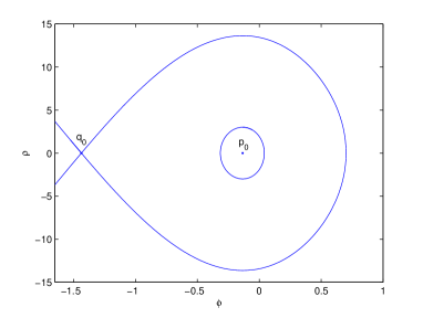
(a)  $\xi=0$

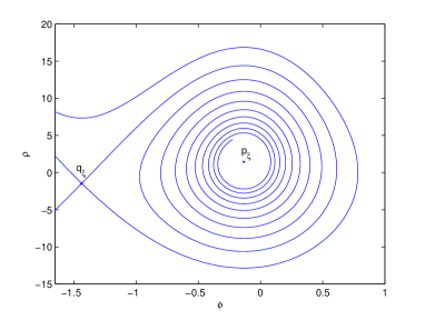
(b)  $\xi=1$

Figure 4: (a) Numerical phase portraits of Eqs. (40) with $\xi=0$ [or equivalently, Eqs. (41)], showing a saddle and a center. (b) Numerical phase portraits of Eqs. (40) with $\xi=1$, showing that the saddle remains a saddle but that the center becomes a sink, with their $\rho$ coordinates shifted slightly down and up, respectively. The parameters are $\delta=2,\Omega=400,h=1,b=0.2649,\gamma=hb\delta$.

Fig. 4(a) shows the phase portrait of Eqs. (41), which contains a saddle $q_{0}$ at $(\rho=0,\phi=\phi_{s}=[\arcsin b-\pi]/2)$, and a center $p_{0}$ at $(\rho=0,\phi=\phi_{c}=-[\arcsin b]/2)$, where $b\equiv\gamma/h\delta$. The fixed points of Eqs. (40) that contain the additional $O(\sqrt{\xi})$ terms are $q_{\xi}=(-\rho_{\xi},\phi_{s})$ and $p_{\xi}=(\rho_{\xi},\phi_{c})$, where $\rho_{\xi}=\sqrt{\xi}3h\sqrt{1-b^{2}}/2$. For small positive $\xi$, a linear analysis of these fixed points reveals that $q_{\xi}$ is still a saddle but that $p_{\xi}$ is a sink, as shown in Fig. 4(b). The fixed points of the full equations (39) near $I=I^{r}$ are the same saddle and sink, located at $(I=I^{-},\phi=\phi_{s})$ and $(I=I^{+},\phi=\phi_{c})$, respectively, where $I^{\pm}=I^{r}\pm\sqrt{\xi}\rho_{\xi}$.

The scaled equations (41) provide an estimate for the basin of attraction of the sink, which is the area confined within the homoclinic orbit connecting the saddle $q_{0}$ to itself, shown in Fig. 4(a). Recall that the dynamics on the unperturbed annulus $\mathscr{M}$ is composed of simple one-dimensional flows, which on resonance turn into a circle of fixed points. Upon adding the small perturbation, two of these fixed points persist in an interval of length $\pi$, and the phase space contains two-dimensional flows. Of particular interest is the basin of attraction of the sink, because a homoclinic orbit to a fixed point of this type offers a mechanism for producing chaotic motion. This mechanism, which results from the existence of a homoclinic trajectory to a saddle-focus fixed point, was described by Šilnikov Šilnikov (1970). Obtaining an estimate for the basin of attraction of the sink, allows us to pick-out the trajectories satisfying Šilnikov’s theorem, which we do in the following section.

VII A HOMOCLINIC CONNECTION TO THE SINK $p_{\xi}$

We are finally in a position to show the existence of an orbit homoclinic to the sink $p_{\xi}$. Note that for a particular set of parameters the existence of such an orbit implies the existence of another symmetric orbit due to the invariance $(x,y)\rightarrow(-x,-y)$. To achieve this, we first show that there exists a homoclinic orbit that approaches $p_{\xi}$ asymptotically backward in time, and approaches the perturbed annulus $\mathscr{M}_{\xi}$ asymptotically forward in time. We then estimate the conditions under which the perturbed counterpart of the point, which is reached on $\mathscr{M}$ forward in time in the unperturbed system, lies within the basin of attraction of the sink $p_{\xi}$ on $\mathscr{M}_{\xi}$. This gives us an estimate for the possibility of obtaining a Šilnikov orbit that connects the sink back to itself.

The first step is done by finding the conditions for which the Melnikov function $M(I^{r},\phi_{0}=\phi_{c}+\Delta\phi/2)$ has simple zeros. We substitute $\phi_{0}=\phi_{c}+\Delta\phi/2$ into the first term in Eq. (36), and recall that $\sin 2\phi_{c}=-b$, to get

$$\sin 2\phi_{0}\sin\Delta\phi=\frac{1}{2}\left[\sqrt{1-b^{2}}(1-\cos 2\Delta\phi)-b\sin 2\Delta\phi\right].$$ (43)

By substituting (43) into the Melnikov function (36) and equating it to zero we obtain the equation

$$3I^{r}\left[\sqrt{1-b^{2}}(1-\cos 2\Delta\phi)-b\sin 2\Delta\phi\right]+2b(3I^{r}\Delta\chi_{1}+3\Delta\mu-2\Delta\sigma)=0,$$ (44)

from which we extract an explicit expression for the condition on $b$, ensuring the existence of an orbit that asymptotes to $p_{\xi}$ backwards in time, and to $\mathscr{M}_{\xi}$ forward in time,

$$|b|=\frac{1-\cos 2\Delta\phi}{\sqrt{\left(\frac{4}{3I^{r}}\Delta\sigma+\sin 2\Delta\phi-2\Delta\chi_{1}-\frac{2\Delta\mu}{I^{r}}\right)^{2}+(1-\cos 2\Delta\phi)^{2}}}.$$ (45)

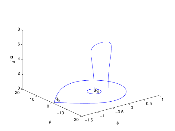
Figure 5: The heteroclinic orbit given by Eqs. (15) with $I=I^{r}$, superimposed with the phase portrait of the unperturbed scaled system on $\mathscr{M}_{\xi}$ near resonance, given by Eqs. (41). The parameters are the same as in Fig. 4(a), with $\Omega_{1}=21.32$. For these parameters $b=0.2949$ according to Eq. (45), so we fix $h=1$ and $\gamma=\delta bh$ in Eqs. (41). This value of $b$ sets $\phi(-\infty)=\phi_{c}=-0.1341$, and as can be seen from the figure $\phi_{s}<\phi(\infty)=\phi_{c}+\Delta\phi<\phi_{m}$.

Next, we wish to find an approximate condition, ensuring that this orbit approaches $p_{\xi}$ as $T\rightarrow\infty$. To do so we find the condition for which the unperturbed heteroclinic orbit, which asymptotes to $p_{0}$ as $T\rightarrow-\infty$, returns back to a point on the circle of fixed points that is inside the homoclinic separatrix loop connecting the saddle $q_{0}$ to itself Kovačič and Wiggins (1992). Such an orbit is shown in Fig. 5. This condition is formulated in terms of the difference $\Delta\phi$ between the asymptotic values of the angular variable $\phi$ as

$$\phi_{s}<\phi_{c}+\Delta\phi<\phi_{m},$$ (46)

where $\phi_{m}$ is the maximal value of $\phi$ on the homoclinic orbit, connecting the saddle $q_{0}$ to itself. Since the Hamiltonian is conserved along an orbit, $\phi_{m}$ satisfies the equation

$$0 = \mathscr{H}(0,\phi_{m})-\mathscr{H}(0,\phi_{s})$$ (47)

$$= 3I^{r}h\delta\left[\frac{1}{2}\sqrt{1-b^{2}}+\frac{1}{2}\cos 2\phi_{m}-b\left(\phi_{m}+\frac{\pi}{2}-\frac{1}{2}\arcsin b\right)\right],$$

whose roots are found numerically to obtain $\phi_{m}$.

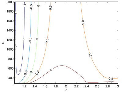
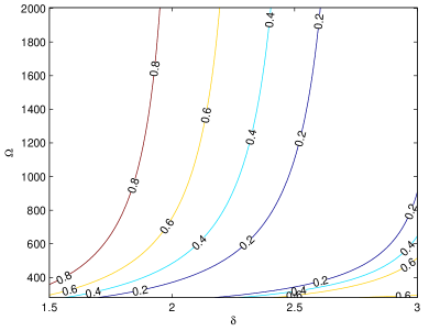
Figure 6: (Color online) (a) Contour plot of the left-hand side of the inequality (48). In the displayed range of $\Omega$, for $\delta\gtrsim 1.5$, this function is positive and the coefficient $\gamma$ represents energy dissipation. For fixed $\epsilon=0.01$ and $1<\delta<3$, the scaled frequency $\Omega_{1}$ reaches values of $0<\Omega_{1}<28$. (b) The ratio $b=\gamma/h\delta$, given by Eq. (45), as a function of $\Omega$ and $\delta$ $(\epsilon=0.01)$. Here $1.5<\delta<3$ and $b$ is positive.

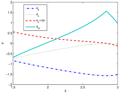
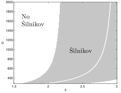
Figure 7: (a) (Color online) The values of $\phi_{s}$, $\phi_{c}$, $\phi_{c}+\Delta\phi$, and $\phi_{m}$ as functions of $\delta$, for $\Omega=1135.64$. For $\delta>2.12$ the condition (46) is satisfied and orbits homoclinic to the sink $p_{\xi}$ exists, except when $\Delta\phi=0$. (b) Parameter values for which the condition (46) is satisfied are indicated in gray. The white line inside the gray area corresponds to $\Delta\phi=0$, where the theory does not apply. In both figures $\epsilon=0.01$.

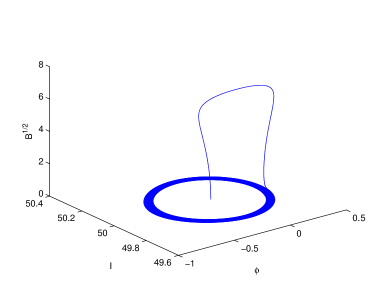
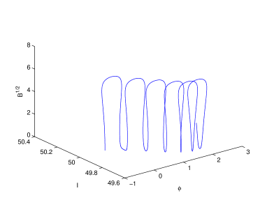
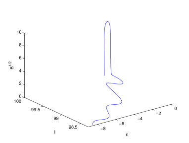
Figure 8: Results of our numerical scheme for $\xi=0.001$ and the rest of the parameters as in Fig. 5. (a) An illustration of the Šilnikov orbit that is obtained for $\gamma=hb\delta$ (The $\xi\rightarrow 0$ limit of this orbit is shown in Fig. 5). For (b) $\gamma=h(b-0.0003)\delta$, and (c) $\gamma=h(b+0.0002)\delta$, and we see that the orbit does not get close enough to $\mathscr{M}_{\xi}$ in order to meet our cutoff criterion for being homoclinic to it. (d) For $\Omega=800$, we obtain an orbit that approaches $\mathscr{M}_{\xi}$ by setting the appropriate value of $\gamma$ $(b=0.6178)$, however, this orbit does not asymptote to the saddle-focus, in agreement with Fig. 7 (b). In this simulation, the orbit leaves $\mathscr{M}_{\xi}$ through its boundary at $I=\Omega_{1}/(\delta-1)$ and eventually $I\rightarrow 0$ and the motion dies out.

Eqs. (45) and (46) define conditions for the existence of orbits homoclinic to the sink $p_{\xi}$. We wish to relate these results to the actual physical parameters of the coupled resonators. Recall that $\delta$ sets the value of the electrostatic coupling coefficient $D=2(\delta^{2}-1)/(3\delta^{2}-1)$. The scaled frequency $\Omega_{1}$ is then given by $\Omega_{1}=(\omega_{1}-\omega_{2})/2\epsilon=(\sqrt{1-D/2}-\sqrt{1-3D/2})/2\epsilon$, so by fixing $\epsilon$ it is also determined by $\delta$. The ratio $b=\gamma/h\delta$, between the damping coefficient and the drive amplitude, has to be positive in order for the damping coefficient $\gamma$ to be positive and have the standard physical meaning of energy dissipation. The ratio $b$ is positive if the inequality

$$\frac{4}{3I^{r}}\Delta\sigma+\sin 2\Delta\phi-2\Delta\chi_{1}-\frac{2\Delta\mu}{I^{r}}>0$$ (48)

is satisfied. We plot the left-hand side of this inequality as a function of $\Omega$ and $\delta$ in Fig. 6(a), and find that it is positive if $\delta\gtrsim 1.5$. Consequently we plot the ratio $b$ in Fig. 6(b) for $1.5<\delta<3$. This value of $b$ then determines the $\phi$ values of the fixed points of Eq. (41), which are shown in Fig. 7(a), along with $\phi_{c}+\Delta\phi$ and $\phi_{m}$ for a particular value of $\Omega$. The parameter values for which these $\phi$ values satisfy the condition (46) are displayed in Fig. 7(b), which outlines the values of the electrostatic coupling and parametric driving frequency, for which orbits homoclinic to the sink $p_{\xi}$ exist. We note that Šilnikov orbits were also found in other two-mode parametrically driven systems Haller and Wiggins (1995); Feng and Sethna (1993); Feng and Wiggins (1993); Zhang (2001), however, slightly different equations were studied, resulting in different phase space dynamics for the unperturbed system as well as different perturbations.

Finally, we wish to verify our calculations by a numerical solution of the ODEs (19). The difficulty in producing a Šilnikov orbit in these equations is that the linearized growth rates of the saddle-focus fixed point—a saddle on the $(B,\theta)$ plane and a focus on the perturbed annulus $\mathscr{M}_{\xi}$—are $O(\xi)$ in directions tangent to $\mathscr{M}_{\xi}$, so the orbit has to spend a lot of time near $\mathscr{M}_{\xi}$ in order to spiral around the saddle-focus. However, the linearized growth rates of this fixed point in directions transverse to $\mathscr{M}_{\xi}$, are $O(1)$, so a small and inevitable numerical error would deflect the orbit away from $\mathscr{M}_{\xi}$. To avoid this problem we solve the ODEs (19) using a cutoff criterion. We initiate the numerical solution with $B\ll 1$, and the exact coordinates of the sink on $\mathscr{M}_{\xi}$, $(I=I^{+},\phi=\phi_{c})$. The orbit initially flows away from $\mathscr{M}_{\xi}$ and later turns around and approaches it. If on its way back towards $\mathscr{M}_{\xi}$, the orbit approaches it close enough to satisfy $B<\xi/1000$, we set $dB/dT=d\theta/dT=0$ in Eq. (19), thus restricting the motion to be tangent to $\mathscr{M}_{\xi}$. This numerical scheme allows us to verify our predictions, because as shown in Fig. 8, only when the damping coefficient is equal to $\gamma=hb\delta$ ($\pm\sim 0.1\%$), with $b$ given by Eq. (45), is our cutoff criterion for eliminating the motion transverse to $\mathscr{M}_{\xi}$ satisfied. Furthermore, as shown in Figs. 8(a) and (d), among the orbits that satisfy our cutoff criterion, only the ones that satisfy the condition (46) asymptote to the saddle-focus.

Owing to a theorem of Šilnikov Kovačič and Wiggins (1992), the existence of orbits homoclinic to a saddle-focus fixed point in Eq. (19) implies that these equations contain chaotic motion in the sense of horseshoes in their dynamics.

VIII SUMMARY

We have studied the origin of chaotic dynamics, and provided conditions for its existence, in a case of two parametrically-driven nonlinear resonators. This was achieved by applying a method of Kovačič and Wiggins on transformed amplitude equations that were derived from the equations of motion, which model an actual experimental realization of coupled nanomechanical resonators. We considered the amplitude of the drive and the damping to be small perturbations and obtained explicit expressions for orbits homoclinic to a two-dimensional invariant annulus in the unperturbed equations. At resonance, we were able to calculate the Melnikov integral analytically, and provide a primary condition for having homoclinic orbits in the full, perturbed equations. By further studying the effects of perturbations on the invariant annulus near resonance, we found a secondary condition for the existence of orbits homoclinic to a fixed point of a saddle-focus type. We used a numerical scheme to verify our theoretical predictions. Such Šilnikov homoclinic orbits give rise to a particular type of horseshoe chaos, which can be expected in the dynamics of the full system for parameter values in the vicinity of those presented here.

References

• Roukes (2001) M. L. Roukes, Scientific American, 285, 42 (2001).
• Cleland (2003) A. Cleland, Foundations of Nanomechanics (Springer, Berlin, 2003).
• Craighead (2000) H. G. Craighead, Science, 290, 1532 (2000).
• Rugar et al. (2004) D. Rugar, R. Budakian, H. J. Mamin,  and B. W. Chui, Nature, 430, 329 (2004).
• Ilic et al. (2004) B. Ilic, H. G. Craighead, S. Krylov, W. Senaratne, C. Ober,  and P. Neuzil, J. Appl. Phys., 95, 3694 (2004).
• Yang et al. (2006) Y. T. Yang, C. Callegari, X. L. Feng, K. L. Ekinci,  and M. L. Roukes, Nano. Lett., 6, 583 (2006).
• Li et al. (2007) M. Li, H. X. Tang,  and M. L. Roukes, Nature Nanotechnology, 2, 114 (2007).
• Naik et al. (2009) A. K. Naik, M. S. Hanay, W. K. Hiebert, X. L. Feng,  and M. L. Roukes, Nature Nanotechnology, 4, 445 (2009).
• Schwab et al. (2000) K. Schwab, E. A. Henriksen, J. M. Worlock,  and M. L. Roukes, Nature, 404, 974 (2000).
• Weig et al. (2004) E. M. Weig, R. H. Blick, T. Brandes, J. Kirschbaum, W. Wegscheider, M. Bichler,  and J. P. Kotthaus, Phys. Rev. Lett., 92, 046804 (2004).
• LaHaye et al. (2004) M. D. LaHaye, O. Buu, B. Camarota,  and K. C. Schwab, Science, 304, 74 (2004).
• Naik et al. (2006) A. Naik, O. Buu, M. D. LaHaye, A. D. Armour, A. A. Clerk, M. P. Blencowe,  and K. C. Schwab, Nature, 443, 193 (2006).
• Rocheleau et al. (2010) T. Rocheleau, T. Ndukum, C. Macklin, J. B. Hertzberg, A. A. Clerk,  and K. C. Schwab, Nature, 463, 72 (2010).
• O’Connell et al. (2010) A. D. O’Connell, M. Hofheinz, M. Ansmann, R. C. Bialczak, M. Lenander, E. Lucero, M. Neeley, D. Sank, H. Wang, M. Weides, J. Wenner, J. M. Martinis,  and A. N. Cleland, Nature, 464, 697 (2010).
• Lifshitz and Cross (2008) R. Lifshitz and M. C. Cross, in Review of Nonlinear Dynamics and Complexity, Vol. 1, edited by H. G. Schuster (Wiley, Meinheim, 2008) pp. 1–52.
• Rhoads et al. (2010) J. F. Rhoads, S. W. Shaw,  and K. L. Turner, J. Dyn. Sys. Meas. Control, 132, 034001 (2010).
• Turner et al. (1998) K. L. Turner, S. A. Miller, P. G. Hartwell, N. C. MacDonald, S. H. Strogatz,  and S. G. Adams, Nature, 396, 149 (1998).
• Zaitsev et al. (2005) S. Zaitsev, R. Almog, O. Shtempluck,  and E. Buks, in Proccedings of the 2005 International Conference on MEMS, NANO, and Smart Systems (ICMENS 2005) (IEEE Computer Society, 2005) pp. 387–391.
• Aldridge and Cleland (2005) J. S. Aldridge and A. N. Cleland, Phys. Rev. Lett., 94, 156403 (2005).
• Kozinsky et al. (2007) I. Kozinsky, H. W. C. Postma, O. Kogan, A. Husain,  and M. L. Roukes, Phys. Rev. Lett., 99, 207201 (2007).
• Buks and Roukes (2002) E. Buks and M. L. Roukes, J. Microelectromech. Syst., 11, 802 (2002).
• Sato et al. (2006) M. Sato, B. E. Hubbard,  and A. J. Sievers, Revs. Mod. Phys., 78, 137 (2006).
• Sato and Sievers (2007) M. Sato and A. J. Sievers, Phys. Rev. Lett., 98, 214101 (2007).
• Sato and Sievers (2008) M. Sato and A. J. Sievers, Low Temp. Phys., 34, 543 (2008).
• Scheible et al. (2002) D. V. Scheible, A. Erbe, R. H. Blick,  and G. Corso, App. Phys. Lett., 81, 1884 (2002).
• DeMartini et al. (2007) B. E. DeMartini, H. E. Butterfield, J. Moehlis,  and K. L. Turner, J. Microelectromech. Syst., 16, 1314 (2007).
• Karabalin et al. (2009) R. B. Karabalin, M. C. Cross,  and M. L. Roukes, Phys. Rev. B, 79, 165309 (2009).
• Kacem et al. (2009) N. Kacem, S. Hentz, D. Pinto, B. Reig,  and V. Nguyen, Nanotechnology, 20, 275501 (2009).
• Kacem et al. (2010) N. Kacem, J. Arcamone, F. Perez-Murano,  and S. Hentz, J. Micromech. Microeng., 20, 045023 (2010).
• Zhang et al. (2002) W. Zhang, R. Baskaran,  and K. L. Turner, Sensors and Actuators A, 102, 139 (2002).
• Buks and Yurke (2006) E. Buks and B. Yurke, Phys. Rev. E, 74, 046619 (2006).
• Cross et al. (2004) M. C. Cross, A. Zumdieck, R. Lifshitz,  and J. L. Rogers, Phys. Rev. Lett., 93, 224101 (2004).
• Cross et al. (2006) M. C. Cross, J. L. Rogers, R. Lifshitz,  and A. Zumdieck, Phys. Rev. E, 73, 036205 (2006).
• Katz et al. (2007) I. Katz, A. Retzker, R. Straub,  and R. Lifshitz, Phys. Rev. Lett., 99, 040404 (2007).
• Katz et al. (2008) I. Katz, R. Lifshitz, A. Retzker,  and R. Straub, New J. Phys., 10, 125023 (2008).
• Liu et al. (2004) S. Liu, A. Davidson,  and Q. Lin, J. Micromech. Microeng., 14, 1064 (2004).
• De and Aluru (2005) S. K. De and N. R. Aluru, Phys. Rev. Lett., 94, 204101 (2005).
• Park et al. (2008) K. Park, Q. Chen,  and Y.-C. Lai, Phys. Rev. E, 77, 026210 (2008).
• Haghighi and Markazi (2010) H. S. Haghighi and A. H. Markazi, Communications in Nonlinear Science and Numerical Simulation, 15, 3091 (2010).
• Wiggins (1988) S. Wiggins, Global Bifurcations and Chaos - Analytical Methods (Springer, Berlin, 1988).
• Melnikov (1963) V. K. Melnikov, Trans. Mosc. Math. Soc., 12, 1 (1963).
• Holmes and Marsden (1982) P. J. Holmes and J. E. Marsden, Commun. Math. Phys., 82, 523 (1982a).
• Holmes and Marsden (1982) P. J. Holmes and J. E. Marsden, J. Math. Phys., 23, 669 (1982b).
• Kovačič and Wiggins (1992) G. Kovačič and S. Wiggins, Physica D, 57, 185 (1992).
• Kovačič (1992) G. Kovačič, Phys. Lett. A, 167, 143 (1992).
• Kovačič (1995) G. Kovačič, SIAM J. on Math. Anal., 26, 1611 (1995).
• Šilnikov (1970) L. P. Šilnikov, Math. USSR Sb., 10, 91 (1970).
• Lifshitz and Cross (2003) R. Lifshitz and M. C. Cross, Phys. Rev. B, 67, 134302 (2003).
• Bromberg et al. (2006) Y. Bromberg, M. C. Cross,  and R. Lifshitz, Phys. Rev. E, 73, 016214 (2006).
• Kenig et al. (2009) E. Kenig, R. Lifshitz,  and M. C. Cross, Phys. Rev. E, 79, 026203 (2009a).
• Kenig et al. (2009) E. Kenig, B. A. Malomed, M. C. Cross,  and R. Lifshitz, Phys. Rev. E, 80, 046202 (2009b).
• Meron and Procaccia (1986) E. Meron and I. Procaccia, Phys. Rev. Lett., 56, 1323 (1986a).
• Meron and Procaccia (1986) E. Meron and I. Procaccia, Phys. Rev. A, 34, 3221 (1986b).
• Feng and Sethna (1989) Z. C. Feng and P. R. Sethna, Journal of Fluid Mechanics, 199, 495 (1989).
• Feng and Sethna (1993) Z. C. Feng and P. R. Sethna, Nonlinear dynamics, 4, 389 (1993).
• Feng and Wiggins (1993) Z. Feng and S. Wiggins, Z. Angew. Math. Phys., 44, 201 (1993).
• Feng and Leal (1995) Z. C. Feng and L. G. Leal, Journal of Applied Mechanics, 62, 235 (1995).
• Zhang (2001) W. Zhang, J. of Sound and Vibration, 239, 1013 (2001).
• Moehlis et al. (2009) J. Moehlis, J. Porter,  and E. Knobloch, Physica D, 238, 846 (2009).
• Kaper and Kovačič (1996) T. J. Kaper and G. Kovačič, Trans. Am. Math. Soc., 348, 3835 (1996).
• Haller and Wiggins (1995) G. Haller and S. Wiggins, Archive for Rational Mechanics and Analysis, 130, 25 (1995).