Spectropolarimetric Signatures of Clumpy Supernova Ejecta

Abstract

Polarization has been detected at early times for all types of supernova, indicating that such systems result from or quickly develop some form of asymmetry. In addition, the detection of strong line polarization in supernovae is suggestive of chemical inhomogeneities (“clumps”) in the layers above the photosphere, which may reflect hydrodynamical instabilities during the explosion. We have developed a fast, flexible, approximate semi-analytic code for modeling polarized line radiative transfer within 3-D inhomogeneous rapidly-expanding atmospheres. Given a range of model parameters, the code generates random sets of clumps in the expanding ejecta and calculates the emergent line profile and Stokes parameters for each configuration. The ensemble of these configurations represents both the effects of various host geometries and of different viewing angles. We present results for the first part of our survey of model geometries, specifically the effects of the number and size of clumps (and the related effect of filling factor) on the emergent spectrum and Stokes parameters. Our simulations show that random clumpiness can produce line polarization in the range observed in SNe Ia ($\sim$1-2%), as well as the Q-U loops that are frequently seen in all SNe. We have also developed a method to connect the results of our simulations to robust observational parameters such as maximum polarization and polarized equivalent width in the line. Our models, in connection with spectropolarimetric observations, can constrain the 3-D structure of supernova ejecta and offer important insight into the SN explosion physics and the nature of their progenitor systems.

1 Introduction

Our understanding of supernovae (SNe) has an impact on a wide variety of astronomical fields, from star formation, interstellar medium dynamics and chemical evolution of galaxies through cosmological models and the distance ladder. Indeed, our dependence on the uniformity of Type Ia SNe (SNe Ia) requires a greater precision of theory than is generally necessary in astronomy. Yet there remain a number of unanswered questions in the field that may impact the accuracy of results obtained from our current models of supernovae. One important aspect of SNe not yet well understood is their asymmetry, which may impact their observed brightness as well as the deposition of kinetic energy and enriched material into their environment.

We have broad indications of SN asymmetry both from theory and from observation. High proper-motion pulsars from SNe, $\gamma$-ray bursts and asymmetric remnants support the idea observationally for core-collapse SNe (Lyne & Lorimer 1994; Woosley & Bloom 2006; Fesen 2001; Hwang et al. 2004); the leading theories of SNe Ia progenitors imply breaking of symmetry due to binarity (Wang & Wheeler 2008), as do the hydrodynamical instabilities and and off-center ignition conditions seen in explosion simulations (Khokhlov et al. 1999; Plewa et al. 2004; Röpke et al. 2007). Further, basic expectations regarding rotation and magnetic fields suggest asymmetries in the progenitor star structure with potentially complicated effects on the resulting ejecta.

Observational probes of SN asymmetries have been challenging. All SNe yet seen in the modern era of astronomical detection have not been resolvable for years after the explosion – the first resolved images of SN 1987A, the closest in modern times, with the Hubble Space Telescope came in 1991 (Podsiadlowski 1991). Further, the most common diagnostic of asymmetry in unresolved sources – line profiles – are not practical in SNe, where ejecta velocities are typically on order of 10,000-20,000 km s^-1 or more. Therefore the most effective way of probing the asymmetries in SNe is with spectropolarimetry.

Polarization tells us about the asymmetries of an unresolved object. In SNe, polarization is generally thought to arise from electron scattering in the last few optical depths within the photosphere. If the source is completely symmetric, all polarization angles will be present in equal quantities, and we will measure no net polarization – the equivalent of “natural light.” If, on the other hand, the source photosphere is asymmetric, or if some of the polarized light is blocked by an asymmetric opacity above the photosphere, different polarization angles will be present in different strengths, and we will detect a net polarization Kasen et al. (2003).

Spectropolarimetry has the potential to give us even more insight into the structure of SN. In supernovae, the velocity of individual mass elements are set within the first few days after the initial explosion. The mass of the ejecta quickly stratifies into a pseudo-Hubble flow, where distance from the center of the explosion is proportional to velocity. Thus, in a SN spectrum, observations at a given wavelength will correspond to the same mass-elements over time. By measuring the variation of polarization with wavelength, we can observe asymmetries as a function of radius, as well as the effects of depolarization by line scattering, giving us information about chemical and density inhomogeneities within the ejecta.

Many observers have contributed to our knowledge of the spectropolarimetric characteristics of SNe (e.g., Leonard et al. 2006; Maund et al. 2007; Chornock & Filippenko 2008; Tanaka et al. 2009). The results are well discussed in Wang & Wheeler (2008), so here we will only state the most general conclusions: Core-collapse supernovae show evidence of an underlying axisymmetric explosion mechanism, and also show significant deviations from that axisymmetry in individual cases. SNe Ia show little continuum polarization and thus are likely close to globally symmetric. SNe Ia absorption lines, on the other hand, are often associated with strong polarization peaks. This can be interpreted as being due to clumpy structures in the outer layers, composed of intermediate mass elements, which asymmetrically block the photosphere.

To understand the host geometry that produced a given spectropolarimetric signature, it is necessary to model radiative transfer through possible ejecta structures and match the results to observations. The problem of modeling SN spectropolarimetry has been approached in a variety of ways over the past few decades. Most codes for modeling spectropolarimetric radiative transfer within the ejecta of SNe Ia, such as HYDRA (Höflich 2005), and SEDONA (Kasen et al. 2006) use a Monte Carlo approach to line and continuum radiative transfer and $\gamma$-ray  deposition within aspherical ejecta to calculate time-dependent spectropolarimetry from a variety of viewing angles. Another approach to SN modeling, developed by Jennifer Hoffman, specifically addresses the interaction of core-collapse SNe with circumstellar material in Type IIn SNe (Hoffman et al. 2005).

These codes are highly detailed and powerful. Yet this complexity also means that they are computationally intensive, making large-scale parameter studies impractical. Since polarization is a second order effect of the geometry, different source configurations may produce the same polarization signature. It is therefore necessary to understand the statistical likelihood of different source configurations producing a given observational signal. This requires systematic modeling of the expected signal given a wide range of source geometry. The large number of model configurations required for reasonable statistics, the three-dimensional nature of the problem, and the wavelength dependent polarization effects combine to pose a significant computational challenge.

Since our goal is to perform just such a parameter study, we have taken a different approach to supernova spectropolarimetric radiative transfer modeling. In the interest of simplicity, we have chosen to focus our simulations on one potential source of SN asymmetry: regions of enhanced line opacity (“clumps”) in the layers above the SN photosphere suggested by the detection of strong line polarization in SNe. If present, the nature of this clumpiness has implications for explosion models of SNe.

The goals of this paper are therefore to calculate the line polarization from inhomogeneous distributions of elements in the ejecta, and to statistically examine how it relates to clump properties. We therefore systematically study the effects of various numbers and sizes of clumps, placed randomly to recapitulate the effects of a range of explosion scenarios as well as those of line-of-sight orientation. To do this, we have developed a fast, flexible approximate semi-analytic code for modeling radiative transfer within 3-D inhomogeneous ejecta. In this paper, we present this code and our methods for statistically analyzing large numbers of simulated spectra, and use them to explore a variety of possible clumpy ejecta scenarios. From the ensemble of resultant Stokes spectra we can determine what ranges of parameters predict observable characteristics that can constrain aspects of the host geometry.

In §2, we describe our code and how we extract observable trends from an ensemble of calculated spectra. In §3, we present the results of our analysis of the effect of number of clumps and clump size. In §4 we summarize the current work and discuss the code’s future potential.

2 Radiative Transfer Code and Analysis Methods

2.1 Model Geometry and Assumptions

The most basic simplifying assumption in the modeling of supernova ejecta is that all the material is moving purely radially and with the velocity of the material increasing linearly with distance from the center of the explosion. We can make this assumption because the energy that feeds the SN expansion is extremely large, and most is input almost instantaneously (on order of a few seconds). Initial shocks and entrained radioactive material will affect the structure of the ejecta for a few days, but such effects will be minimal by the time the SN is detected, on order of 10 days after the explosion (Arnett 1996). Further, the expanding ejecta is unlikely to encounter any significant circumstellar material at this point in expansion, as that material appears to be cleared out by radiation and other pre-explosion dynamics in the years or centuries before the explosion. The main exception to this may be SN IIn (Hoffman et al. 2008, and references therein), which we do not address in our models. The motion of the ejecta can therefore be considered ballistic.

Our model therefore begins with an $N^{3}$ grid extending from $-d_{\rm max}$ to $+d_{\rm max}$ in each dimension in velocity space (see Fig. 1). By the time a SN becomes observable, the ejecta will have stratified by velocity so that this grid is equivalent to a spatial grid at a given time. Because of the linear dependence of velocity on distance, this structure is sometimes referred to as a pseudo-Hubble flow, and has many of the same characteristics of Hubble expansion. Our supernova is centered at $d=0$ and has a photosphere at $d_{\rm phot}$, outside of which is the ejecta through which our radiative transfer is calculated. The SN ejecta is first initialized to a symmetric, smooth optical depth that decreases as a power law from the photosphere ($\rho=\rho_{0}r^{-n_{ej}}$). (See Table 1 for common parameter values used in all simulations reported in this paper.) Regions of enhanced opacity (clumps) are then added, with their particular parameters selected randomly from a range set for a given simulation. Each simulation consists of 1000 spectra in an “ensemble” of realizations with the same parameter ranges. Clump parameters that can be randomly assigned in this way include the number, central optical depth, radii and distance from the photosphere of the clumps ($n_{\rm cl}$, $\tau_{\rm cl}$, $r_{\rm cl}$ and $d_{\rm cl}$, respectively). We do not specifically vary line-of-sight in our results, because given a large ensemble, the random placement of clumps will recapitulate a variety of lines of sight. This simplification greatly reduces computational and analytical complexity.

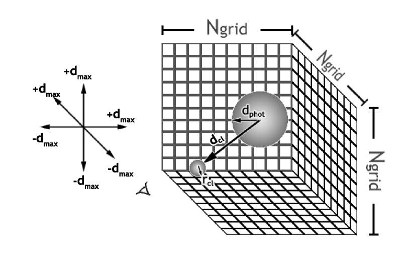
Figure 1: Model grid geometry.

Our Stokes spectra have $N$ wavelength bins centered around a central wavelength, in this case 8000 Å. Note that the exact wavelength is only relevant to the background blackbody spectrum; for these simplified models the “line” is pure trapped resonance scattering and particular line physics are not addressed. $N$ here is the same as the grid dimension.

Our radiative transfer is done in two parts. We begin with the intensity and polarization of the continuum flux, which for a spherically symmetric photosphere can be represented in polar coordinates as

$$\left(\begin{array}[]{ccc}I(r,\phi)\\ \hat{Q}(r,\phi)\\ \hat{U}(r,\phi)\\ \end{array}\right)=\left(\begin{array}[]{ccc}I_{\rm p}(r)\\ I_{\rm p}(r)P_{p}(r)\cos 2\phi\\ I_{\rm p}(r)P_{p}(r)\sin 2\phi\\ \end{array}\right)$$ (1)

where $I_{\rm p}(r)$ is the specific intensity and $P_{\rm p}(r)$ the percent polarization emerging from an impact parameter $r$. The Stokes parameter corresponding to circular polarization, $\hat{V(r,\phi)}$, is taken to be zero, and thus not included in our equations. This is consistent with observations, as no circular polarization has yet been detected in a supernova (Wang & Wheeler 2008). We also use use the Stokes parameter notation given in that paper, where $I$, $\hat{Q}$ and $\hat{U}$ represent the measured vector components, while $Q=\hat{Q}/I$ and $U=\hat{U}/I$ have been normalized. Integrating the intensity over a plane perpendicular to the line of sight gives the Stokes flux at a specific wavelength

$$\begin{split}I&=\int_{0}^{2\pi}d\phi\int_{d_{min}}^{d_{max}}rdr~{}e^{-\tau(r,\phi)}I_{p}(r)+(1-e^{-\tau(r,\phi)})S\\ \hat{Q}&=\int_{0}^{2\pi}d\phi\int_{d_{min}}^{d_{max}}rdr~{}e^{-\tau(r,\phi)}I_{p}(r)P_{p}(r)\cos 2\phi\\ \hat{U}&=\int_{0}^{2\pi}d\phi\int_{d_{min}}^{d_{max}}rdr~{}e^{-\tau(r,\phi)}I_{p}(r)P_{p}(r)\sin 2\phi\end{split}$$ (2)

where $r_{p}$ is the photospheric radius, $d_{min}$ is the impact parameter at which the given plane intersects the photosphere (or zero if the photosphere is not intersected) and $S$ is the line source function, assumed to be pure scattering, $S=W(r,\phi)I_{p}$ where $W$ is the geometrical dilution factor. The plane located at distance $z$ along the line of sight (with a projected velocity $v_{z}$) corresponds to a wavelength $\lambda=\lambda_{0}(1+v_{z}/c)$. In theory, each of these function could have wavelength dependence, but for simplicity over such a small wavelength range we do not vary any of these functions except by letting $I_{\rm p}(\lambda)$ vary according to a blackbody spectrum.

In our simulations, $I_{\rm p}(r)$ and $P_{\rm p}(r)$ are set by the results of a spherical Monte Carlo calculation. Note that for a spherical photosphere, the polarization at the limb is higher than in the plane parallel calculation of Chandrasekhar (1960), used before in e.g., Shapiro & Sutherland (1982). The values of the Q and U Stokes vectors across the observer-oriented face of the photosphere are taken from the model calculated in Kasen et al. (2003).

Equation 2 represents the effect of line opacity above the photosphere in obscuring or diluting continuum flux is calculated. Operationally, for the radiative transfer through the ejecta, we calculate the interacting wavelength for each cell in the 3-D velocity grid using the Sobolev approximation (Sobolev 1960) for line opacity. The light from the photosphere that passes through that cell is then attenuated or scattered at the resonant frequency by the amount determined by the cell optical depth. The combined effects of each cell on all wavelengths gives us our line profile, and asymmetric depolarization of the photospheric flux will give us a spectropolarimetric signal.

Note that we make two main assumptions in this model: First, that there is a clear division between the electron scattering photosphere and the line forming region of clumps. In reality, there is no sharp division, and some electron scattering will be coincident with the line scattering. However, if the clumps can be represented as sufficiently detached from the photosphere, this model will still provide relevant results (see discussion in Kasen et al. 2003).

Second, we make the common assumption that all line scattered light is depolarized. Though this is certainly a simplification of the physical picture, it is a reasonable approximation in most cases. The reasoning given in Hoeflich et al. (1996) is that collisional timescales are less than those for absorption and re-emission in the ejecta; thus the random scattering processes will erase incoming geometrical information for an absorbed photon. We add that even if collisions are not dominant, line polarization is unlikely to be significant because lines are at best weakly polarizing, comparatively (Hamilton 1947) with the greatest polarization in the side scattering case. In our geometry, photons that are side scattered into the line of sight will be seen in the emission portion of the line, while observed polarization is in the absorbed part of the line. Further, any light line-scattered into the line of sight will be a small contribution to the total flux, making such a signal harder to detect.

Thus in our model, polarized rays of light from a pre-computed spherical photosphere are obscured by clumps of depolarizing line opacity. Because the clumps block the photosphere in an asymmetrical way at different velocities, they give rise to polarization over the line flux absorption feature.

Table 1: Model parameters used for simulations in this paper. Sizes are given in velocities, which are proportional to distances in the homologous flow of SN ejecta (see 1).

Parameter	Value
N	100
$d_{\rm max}$	20,000 km s-1
$d_{\rm phot}$	10,000 km s-1
TBB	13,000 K
$\tau_{\rm cl}$	10
$\lambda_{\rm cent}$	8000Å
$n_{\rm ej}$	8

Results from our code have been compared to those of Kasen’s previous semi-analytic codes (Kasen et al. 2003) with the same host configurations, to good agreement. See Hole (2009) for more details. Flux and polarization spectra and Q-U diagrams for three sample realizations are shown in Figures 3, 4 and 5.

2.1.1 Regimes in $n_{\rm cl}$-$r_{\rm cl}$ Parameter Space

The code can be run with any number or size of clumps, but it is worth examining what is physically implied by different regions of $n_{\rm cl}$-$r_{\rm cl}$ parameter space. In the small-clump limit, we are modeling small regions of enhanced concentration of an element, surrounded by smooth ejecta which contribute the bulk of the line profile but no net polarization. As the clumps become larger or more numerous, the model more closely resembles large scale variations in the chemical composition of the overall ejecta structure. Eventually, however, the simulations with the most and largest clumps will completely fill the model grid, and represent a substantial change to the nature of the ejecta, rather than a perturbation of it, to a degree not supported by observation.

Thomas et al. (2002) attempted to constrain clump size and filling factor using line flux profiles only. Comparing results of a numerical clump model to observations of the Si II line, they concluded that clumps larger than 0.08 times the photospheric radius (1600 km s^-1 in our model) would create line-of-sight variations larger than what was seen. Their model was substantively different from ours, however, as they represented clumps as optically thin and surrounded by zero line opacity. The line profile is thus due entirely to the clumps, rather than clumps being a perturbation on the line structure. Therefore in our model, the line-of-sight effects will be smaller even for large clumps, and should have less variation with angle as long as there are enough clumps to fill a majority of the ejecta.

In an attempt to quantify the useful parameter limits in our model, we use a metric based on the photodisk covering factor (PCF) used by Thomas et al. (2002), which they define as the ratio of the area obscured by clumps contained in the projected photodisk area to the total photodisk area for each plane of common velocity along the line-of-sight. The sum of the ratios over all velocities gives a measure of volume filling factor for the ejecta. For these simulations, there are 50 velocity planes on the observer side of the grid, so the sum of the ratios has a maximum of 50 if each plane has 100% of the available photodisk covered.

We therefore delineate four regions of parameter space in our model, as shown in Fig. 2:

1. The small-clump regime, $r_{\rm cl}$ $\leq$ 1600 km s^-1, used by Thomas et al. (2002)

2. Medium-clump regime with smaller filling factor (PFC $<$ 38)

3. Medium-clump regime with larger filling factor (38 $\leq$PCF $<$ 48)

4. Full ejecta (PFC $\geq$ 48)

Region I has small clumps and is numerically and physically plausible. Regions II and III have more substantial clumpiness. In Region II the ejecta is less full, which might lead to greater line-of-sight variation than is seen in observations. Region III has a higher filling factor and thus fewer line-of-sight effects, but also results in more clump overlap, implying the possibility of more complex polarization effects that may not be completely captured with our simplified radiative transfer. Region IV represents a full numerical grid and is not likely to occur in SNe but is shown here to demonstrate the behavior of the model in extreme cases.

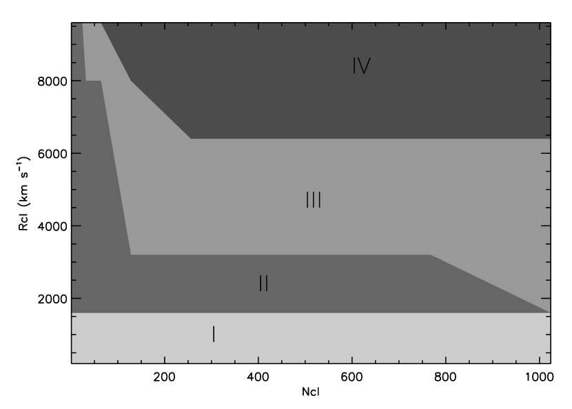
Figure 2: Regions of $r_{\rm cl}$-$n_{\rm cl}$ parameter space. Region I represents the small-clump limit, with $r_{\rm cl}$ $\leq$ 1600 km s^-1. Regions II and III represent medium-sized clumps, with a smaller ejecta filling factor in Region II and greater clump overlap in Region III. Region IV is the filled-ejecta, theoretical limit of the model.

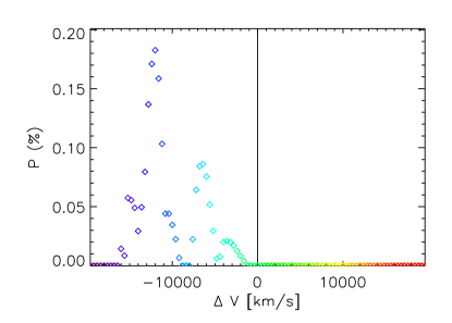
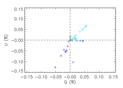
Figure 3: A calculated line profile, spectropolarization profile and Q-U diagram for the $n_{\rm cl}$=32, $r_{\rm cl}$=1600 km s^-1 case. This particular realization has several clumps in the line-of-sight and therefore has a number of broad polarization peaks and distinct variations from a single dominant axis in the Q-U plane.

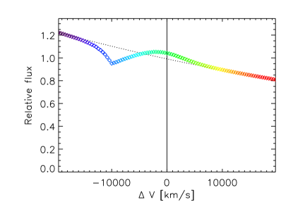
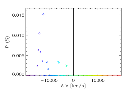
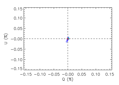
Figure 4: A calculated line profile, spectropolarization profile and Q-U diagram for the same clump configuration as in figure 3 but with $r_{\rm cl}$=400 km s^-1 instead of 1600 km s^-1. Note that the polarization peaks are significantly narrower and $\gtrsim 10$ times smaller in magnitude.

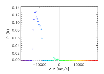
Figure 5: Another calculated line profile, spectropolarization profile and Q-U diagram for the $n_{\rm cl}$=32, $r_{\rm cl}$=1600 km s^-1 case (e.g., it is from the same ensemble as the example in figure 3). This particular realization produces a classic “loop” in the Q-U plane. The difference that leads to this loop is hinted at by the plots of percent polarization: in figure 3, the clumps are separated in velocity space, so the Q-U diagram shows distinct deviations from zero, with a separate position angle for each clump. In contrast, the clumps in this realization are overlapping in velocity and wavelength, so the Q-U diagram shows a smooth varying from one clump’s position angle to another, creating a “loop” structure.

2.2 Analysis of Spectra

Given that each simulation creates an ensemble of 1000 individual Stokes spectra, we developed tools to analyze and visualize the results in a statistical way. We therefore calculate certain salient, observable numbers from each spectrum, and determine the “expected value” for each configuration. The numbers calculated from each spectrum are minimum flux and the velocity and polarization where it occurs; maximum percent polarization ($P$, see eqn. 3) at any frequency in the spectrum ($P_{\rm max}$); polarized equivalent width, Q-vector equivalent width, U-vector equivalent width, and Stokes equivalent width (PEW, QEW, UEW and SEW, see eqn. 4); and theoretical covering fraction (TCF, eqn. 5).

The polarization is defined as

$$P=\frac{\sqrt{{\hat{Q}}^{2}+{\hat{U}}^{2}}}{I}=\sqrt{Q^{2}+U^{2}}$$ (3)

We also define a polarized version of line equivalent width:

$$\mathrm{[X]EW}=\sum\%\mathrm{X}_{\lambda}\left(\frac{\mathrm{I}_{c,\lambda}-\mathrm{I}_{\lambda}}{\mathrm{I}_{c,\lambda}}\right)\Delta\lambda,$$ (4)

where [X] can be P, Q, or U and $\mathrm{I}_{c}$ is the continuum flux. Since QEW and UEW should each be sampling the same underlying distribution even if their values differ in a given spectrum, we add these separate distributions together to double the sample size. We call this combined value “Stokes equivalent width,” or SEW. In this paper, we focus primarily on the analysis of $P_{\rm max}$ and PEW results.

The concept of the “theoretical” covering fraction is also worthy of more discussion. It is useful to have a way of calculating a covering fraction in order to facilitate comparison to the results of explosion codes; however the correct measure of covering fraction in our simulations is not as simple as one might expect. First, our randomly placed clumps may not be in the line of sight, and therefore may not in that sense be “covering” the photosphere from the observer’s point of view. However, to most easily compare our results with the predictions of explosion codes, we need to account for the total number of clumps. Further, because our clumps are distributed in velocity space, the covering fraction will be different at different frequencies depending on where the Sobolev line interaction occurs. The covering fraction at each wavelength in the line of sight can be calculated (e.g.,the “photodisk covering fraction” of section 2.1.1) however this measure is not ideal here because it is a) a spectrum rather than a single number, b) subject to line-of-sight effects and c) more complicated to compare to explosion models. We therefore have chosen to use the theoretical covering fraction, which we define as follows:

$$\mathrm{TCF}=\sum_{N_{\rm cl}}\frac{\pi r_{\rm cl}^{2}}{4\pi d_{\rm cl}^{2}}$$ (5)

In words, we find the fraction each clump subtends of the total area of the sphere located at the distance of the clump, and then take the sum of these fractions for all clumps. There are limitations to this method, particularly in that our clumps may overlap either within the opacity grid or in line of sight, and may therefore overestimate the covering fraction, potentially creating a TCF that is greater than one, even if there are some locations or wavelengths where the photosphere is unobscured. It does, however, create a single, conceptually clear number to use in calculations and comparisons.

2.3 Analysis of Ensembles

Once the appropriate metrics are calculated for each individual spectrum in an ensemble, we can perform statistical analysis on the results. If we have 1,000 realizations of a given set of parameters, we have 1,000 predictions of, for instance, the maximum polarization that could be produced by that configuration. A Gaussian fit to a histogram of the maximum polarizations thus produced allows us to predict the likelihood of a given polarization being produced by that geometry. We can also use such model parameters as number of clumps ($n_{\rm cl}$), clump size ($r_{\rm cl}$) or TCF to connect these geometries to those predicted by different SNe explosion modeling codes, and thereby determine what spectropolarimetric signatures these explosion codes would imply in our simulations.

In Figure 6 we show some of the statistical results for an ensemble, namely the histograms of $P_{\rm max}$ and SEW. In this ensemble, clumps were randomly distributed between the photosphere and the edge of the grid, and with $n_{\rm cl}$=16 and $r_{\rm cl}$=1600 km s^-1. Additional parameters are as in Table 1.

Analysis of such histograms can lead to insights into the factors contributing to the overall distribution. In this ensemble, we see three main contributions. First, the peak at zero polarization represents a combination of symmetrically placed clumps and instances where the clumps were randomly placed so that none of them lie in the line-of-sight. Between zero and $\sim$0.15% we see a steadily increasing slope that make up the bulk of the asymmetric population, following the expected properties of clump distribution. Third, in addition to this bulk population, there are a small number of outliers in the distribution. These outliers have the potential to demonstrate interesting though unlikely configurations, and possibly to distinguish between similar clump models.

In addition to analysis of individual ensemble distributions we seek to understand the way our results change with variations of simulation parameters. To see trends in metrics between ensembles, we must find ways to characterize each distribution in ways easily comparable to others with different parameters. One measure we use is a Gaussian fit the distribution, which gives a center and a width. The true mode of the distribution is also calculated, and finally, for some metrics, we find the mode of the distribution if zero is excluded. This second mode can be useful in distributions that can have a peak at zero due to, for example, no clump falling within the line-of-sight, which is distinct from the behavior of the metric when any clumps are in position to affect the observed signal. This second, non-zero mode would therefore be useful for metrics that are not expected to be zero when there are any asymmetries present (e.g., polarized equivalent width) but not for metrics where expected values should be distributed about zero (e.g., $Q_{\rm max}$).

As an example, we again take the case of $P_{\rm max}$ in the line as shown in Figure 6. Here, the Gaussian fit is not a complete representation of the underlying distribution. Indeed, since P is an intrinsically positive quantity, the distribution of P measurements in an ensemble should not be Gaussian by definition. For this metric, the mode seems to be a better measure of the behavior of the distribution produced by our simulation. Unfortunately, the mode cannot capture the width of the distribution, only its most likely value.

In contrast, there are some metrics where the distribution of measurements is more usefully represented by the Gaussian fit than by the mode. Both Q and U individually are expected to be randomly distributed about zero, and thus the combination of the two distributions should be as well. We therefore expect that this data will be more accurately represented by a Gaussian fit. In Figure 6 we show that the distribution of Stokes equivalent width for the same ensemble is indeed more accurately fit by the Gaussian than was the $P_{\rm max}$. Here the width of the fit is a more useful quantity than the mode, which will be at or very close to zero.

Figure 6: The histogram and Gaussian fit for the maximum polarization produced at any point in the line profile (above) and Stokes equivalent width (below) for an ensemble with $n_{\rm cl}$=16 and $r_{\rm cl}$=1600 km s^-1. In the $P_{\rm max}$ plot, the peak at zero represents the combination of symmetrically placed clumps and instances where no clumps appear in the line of sight. The Gaussian fit was set to avoid this peak; the mode of the distribution is calculated for the full distribution, and again excluding the peak at zero. In this case, both modes are the same. Note that the Gaussian fit is a better representation of Stokes equivalent width data than for $P_{\rm max}$, as expected, because Stokes equivalent width should be scattered about zero.

2.4 Inter-Ensemble Parameter Studies

Finally, in order to investigate the effect of different variables on the predicted spectropolarimetric signals we calculate a series of ensembles holding all parameters constant except one. We refer to the resulting set of ensembles as a “run.” To visualize the effects of that parameter, in Figures 8 to 13 we plot the the Gaussian fit parameters and modes determined for each metric in each ensemble versus the varyied parameter. The width of the Gaussian is shown by the gray area. We plot the true mode for zero-centered metrics (i.e. Stokes equivalent width) and non-zero mode for metrics that are not expected to be inherently symmetric.

3 Results

We have performed a preliminary survey of the effect of three interrelated factors on the spectropolarimetric signatures of SNe: clump size, number of clumps and TCF. We note that in addition to likely parameter values, for some of these simulations we use numbers or sizes of clumps that are at physical extremes in order to explore the theoretical limits of the models. (For instance, an ensemble with 1024 clumps of radius 8000 km s^-1 would not be best characterized as representing a “clumpy ejecta,” but can provide insight into trends in the model. See Section 2.1.1.)

In this paper we present complete results for seven runs: two have constant $r_{\rm cl}$ and vary $n_{\rm cl}$ (parameters in Table 2), two have constant $n_{\rm cl}$and vary $r_{\rm cl}$(Table 3), and three vary both $r_{\rm cl}$and $n_{\rm cl}$systematically to maintain an approximately constant TCF (Table 4). For each of these runs we show trends for several metrics.

3.1 Constant $r_{\rm cl}$

We conducted two runs with constant clump radius, one with $r_{\rm cl}$=3200 km s^-1 and the other with $r_{\rm cl}$=6400 km s^-1  (see Table 2 as well as Table 1 for complete parameters).

In our clump model, polarization of SNe is due to asymmetric obscuring of the photosphere (see §LABEL:S:geometry). We expect an increase in polarization as the number of clumps increases. But beyond a certain point, added clumps will create symmetries with other clumps, and the polarization signal will decrease. Therefore we begin by looking for this pattern of increasing polarization at small $n_{\rm cl}$ followed decreasing polarization at large $n_{\rm cl}$. While this behavior is not readily apparent in the $r_{\rm cl}$=3200 km s^-1 run (Figure 7), it is seen in the $r_{\rm cl}$=6400 km s^-1 series (Figure 8). This is likely due to the fact that larger clumps will cover a broader range of Q and U vectors, meaning that it is easier to regain symmetry with fewer clumps.

In the $P_{\rm max}$ versus $n_{\rm cl}$ plot of Figure 7 we have overlaid a fit to the linear portion of the $P_{\rm max}$ data, which has a slope of 0.33. A similar set of plots for $r_{\rm cl}$=6400 km s^-1 are shown in figure 8; the slope of the central approximately linear portion of the $P_{\rm max}$ versus $n_{\rm cl}$ plot is similar, 0.32.

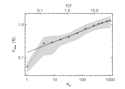
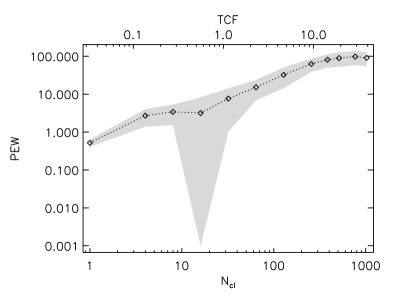
Figure 7: The dependence of $P_{\rm max}$ and PEW on $n_{\rm cl}$ in the $r_{\rm cl}$=3200 km s^-1 run. A fit to the linear power-law portion (slope is 0.33) is plotted in the $P_{\rm max}$ figure (above). TCF of the ensemble is shown, at the top of each figure.

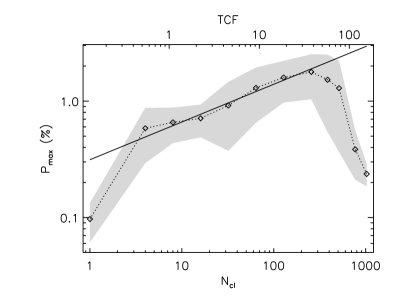
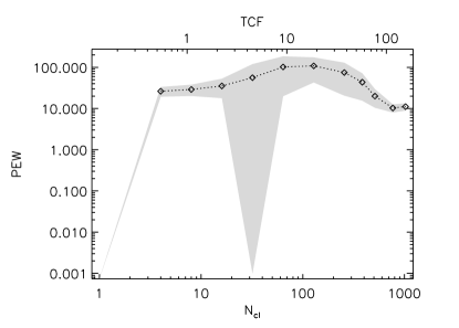
Figure 8: The dependence of $P_{\rm max}$ and PEW on $n_{\rm cl}$ in the $r_{\rm cl}$=6400 km s^-1 run. A fit to the linear power-law portion (slope is 0.32) is plotted in the $P_{\rm max}$ figure (above). Compared to the $r_{\rm cl}$=3200 km s^-1 run (Figure 7) we see significant deviation from power-law behavior at large numbers of clumps, indicating that symmetric areas of the photosphere are being covered by the larger clumps. TCF of the ensemble is shown, at the top of each figure.

3.2 Constant $n_{\rm cl}$

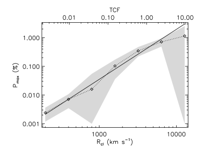
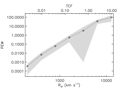
Figure 9: The dependence of $P_{\rm max}$ and PEW on $r_{\rm cl}$ in the $n_{\rm cl}$=16 run. A fit to the linear power-law portion (slope is 1.74) is plotted in the $P_{\rm max}$ figure (above). TCF of the ensemble is shown, at the top of each figure.

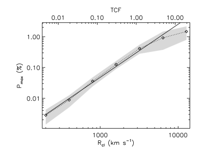
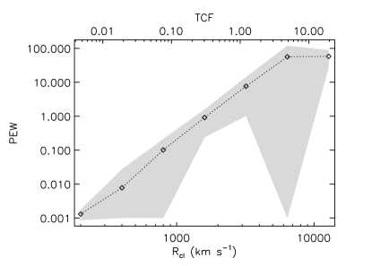
Figure 10: The dependence of $P_{\rm max}$ and PEW on $r_{\rm cl}$ in the $n_{\rm cl}$=32 run. A fit to the linear power-law portion (slope is 1.72) is plotted in the $P_{\rm max}$ figure (above). TCF of the ensemble is shown, at the top of each figure.

We conducted two runs with a constant number of clumps, one with $n_{\rm cl}=16$ and the other with $n_{\rm cl}$=32 (see Table 3 as well as Table 1 for complete parameters).

Figures 9 and 10 show that in the constant $n_{\rm cl}$ runs $P_{\rm max}$$\propto$$r_{\rm cl}$. At larger $r_{\rm cl}$ this relationship breaks down due to increasing geometrical effects from clump overlap, both spatially in the line-of-sight and spectrally in velocity space. In the $P_{\rm max}$ versus $r_{\rm cl}$ plots of Figures 9 and 10, we have overlaid a fit to the linear portion of the data. The slopes are 1.74 and 1.72, respectively.

3.3 Constant TCF

For this series of runs, we held the theoretical covering fraction (TCF, see §2.3 for definition) constant, varying $n_{\rm cl}$from 1 to 1024 and $r_{\rm cl}$ proportionately to maintain a TCF of $\approx 0.15$, $\approx 0.60$ and $\approx 2.4$. The actual TCF obtained for each ensemble is closest to the nominal value at higher $n_{\rm cl}$ where the value is less likely to be skewed by random placements of clumps. Figures 11, 12 and 13 all show that, as anticipated, large numbers of small clumps leads to recapturing symmetry and a decrease in polarization.

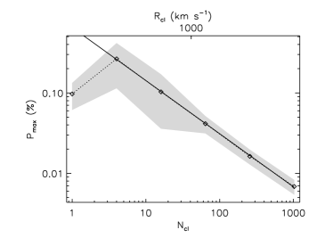
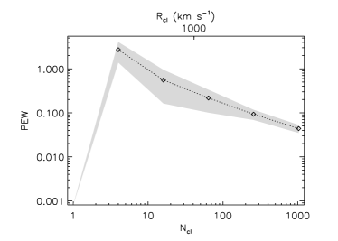
Figure 11: The dependence of $P_{\rm max}$ and PEW on $n_{\rm cl}$ and $r_{\rm cl}$ in the TCF$\simeq 0.15$ run. Linear fits are $\propto-0.66$$n_{\rm cl}$ and $\propto 1.32$$r_{\rm cl}$.

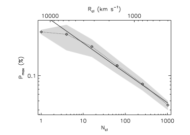
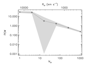
Figure 12: The dependence of $P_{\rm max}$ and PEW on $n_{\rm cl}$ and $r_{\rm cl}$ in the TCF$\simeq 0.60$ run. Linear fits are $\propto-0.55$$n_{\rm cl}$ and $\propto 1.11$$r_{\rm cl}$.

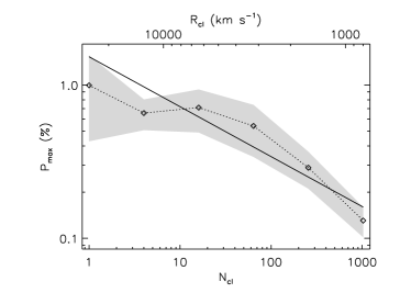
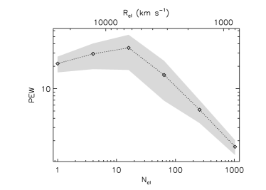
Figure 13: The dependence of $P_{\rm max}$ and PEW on $n_{\rm cl}$ and $r_{\rm cl}$ in the TCF$\simeq 2.4$ run. Linear fits are $\propto-0.33$$n_{\rm cl}$ and $\propto 0.65$$r_{\rm cl}$.

In Figures 11, 12 and 13 we show the log-log plots for the TCF $\simeq~{}0.15$, TCF $\simeq~{}0.60$ and TCF $\simeq~{}2.4$, respectively. In these plots, we have overlaid fits to the linear portions of both $P_{\rm max}$ plots. In the TCF $\simeq 0.15$ case, we find that this slope is 1.32 in the $r_{\rm cl}$ plot and -0.66 in the $n_{\rm cl}$ version; for TCF $\simeq 0.60$ they are 1.11 and -0.55 respectively. In the $\simeq 2.4$ run, a fit to the data gives slopes of 0.65 for $r_{\rm cl}$ and -0.33 for $n_{\rm cl}$, though the behavior no longer appear to be truly linear, due to complicated effects of overlapping of clumps.

In the constant $r_{\rm cl}$ and $n_{\rm cl}$ runs (§3.1 and §3.2), the slope of the fit to the $P_{\rm max}$ remained the same between runs, at least in the portions that are roughly linear. The TCF runs show less uniformity (even excluding the highest TCF run where behavior does not seem linear) than in the other cases. This may indicate a trend where increased covering fraction leads to a flattening of polarization dependence in both $r_{\rm cl}$ and $n_{\rm cl}$.

The difference between the TCF $\simeq 0.15$ and TCF $\simeq 0.60$ is likely due to small statistical variations at very small covering fraction. We therefore take the results from the TCF $\simeq 0.60$ run as most representative of the regime of power-law behavior for the TCF runs, where there are enough clumps for reasonable statistics, but not so many that complex overlapping effects make the polarization dependence non-linear.

3.4 Polarization dependence on $n_{\rm cl}$ and $r_{\rm cl}$

In order to understand these results, we seek a simple model for the relationship between polarization and $n_{\rm cl}$, $r_{\rm cl}$ and TCF. We therefore propose the following simple analytical model and compare it to our model’s numerical behavior in order to test consistency. and to provide insight into both simple and complex regimes.

We begin our proposed model with the polarization due to one clump, $P_{\rm cl}$. The polarization from that clump will depend on the photospheric area covered by the clump, $\propto r_{\rm cl}^{2}$. But the polarization will also depend on what portion of the photosphere is covered – if the clump is very large, it will eventually cover orthogonal vectors in Q-U space, and therefore reduce the polarization due to that clump. Thus we make the assumption that the polarization due to the clump will be proportional to the area of the clump times an unknown function of $r_{\rm cl}$, which we in turn assume to be a power of $r_{\rm cl}$:

$$P_{\rm cl}\propto r_{\rm cl}^{2}f(r_{\rm cl})\propto r_{\rm cl}^{2}r_{\rm cl}^{m}$$ (6)

The polarization should also be a function of $n_{\rm cl}$, which should be roughly linear for small covering fractions. As we increase the number of clumps, we will begin to have more than one clump at the same velocity, each covering different Q and U vectors. While $\langle Q\rangle=0$, $\langle Q^{2}\rangle$ is not. Like a random walk, $Q^{2}\propto n_{\rm cl}$. The same is true for U. Thus, since $P=\sqrt{Q^{2}+U^{2}}$ (equation 3), the total polarization will also increase as $\sqrt{n_{\rm cl}}$. (A similar derivation of the $P\propto\sqrt{n_{\rm cl}}$ behavior is shown in Richardson et al. (1996).) Thus in our model, the total polarization will depend on the number of clumps and the polarization per clump:

$$P_{tot}\propto g(n_{\rm cl})P_{\rm cl}\sqrt{n_{\rm cl}}$$ (7)

Here $g(n_{\rm cl})$ is an as-yet unspecified function of $n_{\rm cl}$ representing the non-linear effects on the total polarization due to multiple clumps. Assuming that $g(n_{\rm cl})\propto n_{\rm cl}^{l}$ and combining equation 7 with equation 6 this becomes

$$P_{tot}\propto n_{\rm cl}^{l}r_{\rm cl}^{m}n_{\rm cl}^{1/2}r_{\rm cl}^{2}=n_{\rm cl}^{l+1/2}r_{\rm cl}^{m+2}$$ (8)

Equation 8 predicts that within a run, the total polarization should have a power-law dependence on $r_{\rm cl}$ and $n_{\rm cl}$. This prediction agrees with the behavior of our models shown in §3.1 and §3.2. The actual dependence can be disentangled by holding either $r_{\rm cl}$ or $n_{\rm cl}$ constant:

$$P_{tot}\propto\left\{\begin{array}[]{rcl}r_{\rm cl}^{m+2}&{}\hfil&\mbox{ for const. $n_{\rm cl}$~{}}\\ n_{\rm cl}^{l+1/2}&{}\hfil&\mbox{ for const. $r_{\rm cl}$~{}}\end{array}\right.$$ (9)

We can now use our simulations to determine the values of $l$ and $m$. The metric that will most directly correspond to the $P_{tot}$ derived above will be $P_{\rm max}$  because it is less influenced by complicated geometry effects in the line. (PEW should also follow this relationship in cases where polarization is due to a few discrete clumps.)

From our simulations, the slope of $P_{\rm max}$ as a function of $n_{\rm cl}$ for constant $r_{\rm cl}$ is 0.33 (Figure 7). Thus $n_{\rm cl}^{l+1/2}=n_{\rm cl}^{0.33}$, and $l=-0.17$. Our results for constant $n_{\rm cl}$ (Figure 9) show $P_{\rm max}$ as a function of $r_{\rm cl}$ is $\propto r_{\rm cl}^{1.74}=r_{\rm cl}^{m+2}$, and so $m=-0.26$.

To check for consistency, we can use our model and these results to predict the behavior of $P_{\rm max}$ for runs with constant TCF. For constant TCF, $n_{\rm cl}r_{\rm cl}^{2}$ is constant, and $n_{\rm cl}\propto r_{\rm cl}^{-2}$ and $r_{\rm cl}\propto n_{\rm cl}^{-1/2}$. Substituting these relations into eqn. 8 we find

$$P_{tot}\propto\left\{\begin{array}[]{l}r_{\rm cl}^{1.08}\\ n_{\rm cl}^{-0.54}\end{array}\right\}\mbox{const. TCF }$$ (10)

These predicted slopes agree remarkably well with the fit to our numerical results: $r_{\rm cl}^{1.11}$ and $n_{\rm cl}^{-0.55}$ (Figure 12).

Note that this implies that the total polarization is decreased by $n_{\rm cl}$^-0.17 if there is substantial clumping. Similarly, total polarization is decreased by $r_{\rm cl}$^-0.26. This implies that the larger the radius of the clump, the more likely it is to extend into less polarized parts of the photosphere or cover complementary Q and U vectors, and thereby reduce the resulting polarization per clump.

Similar behavior for the polarization can be derived by introducing clumps to the integrals in equations 1 and 2. For non-overlapping, optically thick clumps, the average polarization would be propto $n_{\rm cl}^{-1/2}$ and propto $r_{\rm cl}^{1}$. The difference from these values in our results is due to the more complicated effects, such as overlap and velocity-width of the clumps, that can be handled more effectively in the numerical model.

3.5 Connection to Observations

One of the greatest obstacles to the effective use of spectropolarimetry in astrophysics is the degeneracy between source and signal – because polarization is a second order effect, there will likely be more than one host configuration that will produce a given observation. One of the most important goals of this paper is to find ways to break polarimetric degeneracy where possible, and otherwise to estimate the range of possible configurations leading to an observation, and their relative likelihoods.

Two factors that can break degeneracy in polarimetry are wavelength and time dependence. For instance, while continuum polarization for an ellipsoidal photosphere may be the same as that for a spheroidal photosphere with chemically inhomogeneous ejecta, the wavelength dependence of the polarization will be different. The former case will also likely maintain the same degree of polarization and position angle over time, while in the latter, individual clumps will continually become optically thin over time as the ejecta expands, likely resulting in variation in both degree and orientation of polarization.

Our code incorporates the first of these factors intrinsically, namely wavelength dependence in the line profile. Degeneracies for a single SN can be further constrained using observations at different epochs. Take, for instance, the case where one epoch of observations indicate that the asymmetry may be due to a single large clump covering most of the photosphere, or to several overlapping medium-sized clumps at about the same distance from the photosphere. As the ejecta expands, the outer portions of the clumps will become optically thin while the portion of each clump closest to the photosphere may remain optically thick. In later observations of the single-clump case, we would observe the signature of one clump reducing in size. With several overlapping clumps, as we see further towards the center of the SN the single clump would appear to break up and the spectropolarimetric signature would become that of several small clumps. Our simulations predict that this difference should be detected in the relative change in $P_{\rm max}$ and PEW at different epochs.

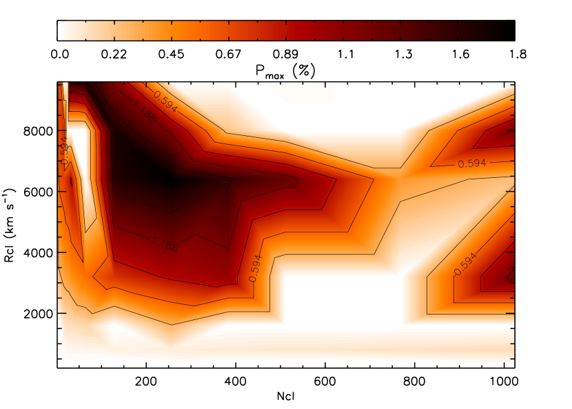
Figure 14: The expectation value of $P_{\rm max}$ as a function of $n_{\rm cl}$ and $r_{\rm cl}$ predicted by our simulations. Here, a measurement of $P_{\rm max}$ in a SN line would be a plane, constraining the host system’s parameters to those described by an intersecting contour in the above plot.

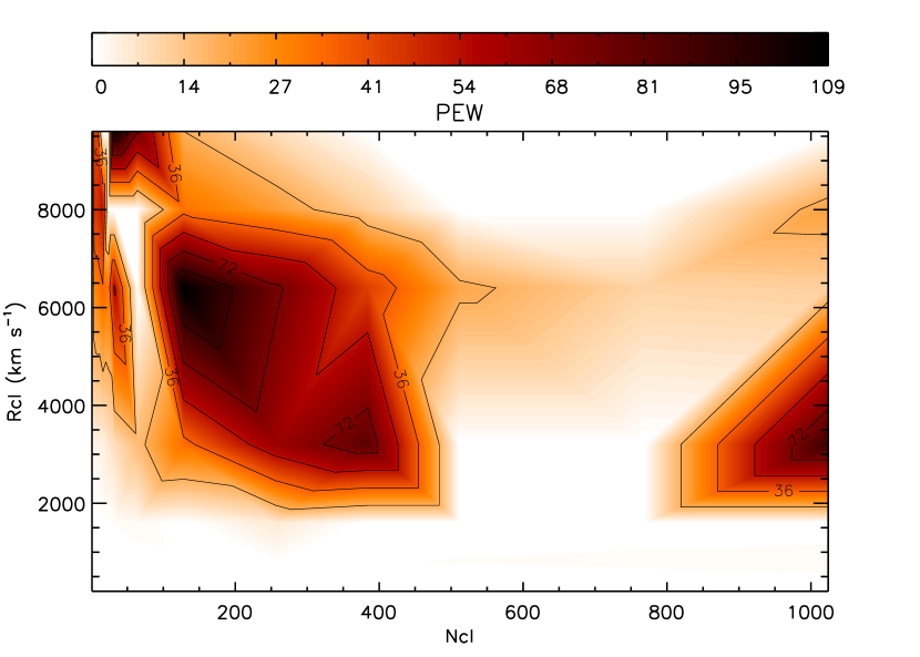
Figure 15: The expectation value of PEW in the line as a function of $n_{\rm cl}$ and $r_{\rm cl}$ predicted by our simulations. Here, a measurement of PEW in a SN line would be a plane, constraining the host system’s parameters to those described by an intersecting contour in the above plot. See the caption of Figure 14 for a description of the dashed and cross-hatched regions.

More directly, our simulations also give us a powerful method of constraining clump parameters by using observational metrics from the same epoch. Using our results from across all of our runs, we can create a map of a metric, such as $P_{\rm max}$, as a function of $n_{\rm cl}$ and $r_{\rm cl}$ (Figure 14). This map will have the form of a topographical map, though rather than having a single value at each point, the surface would have a thickness representing the likely range of $P_{\rm max}$ from our Gaussian fit for that ($n_{\rm cl}$,$r_{\rm cl}$). An observational measurement of $P_{\rm max}$ in the line would be a plane, also with a thickness representing the uncertainty in the measurement. That plane would intersect our map, constraining the source $n_{\rm cl}$ and $r_{\rm cl}$ to the contour thus created. The intersection of uncertainties from our model and observations would give an uncertainty on the prediction.

This method becomes even more powerful when we use more than one metric: the intersection of observed polarized equivalent width with our model (Figure 15) would create another contour in $r_{\rm cl}$ and $n_{\rm cl}$, and the two contours could be combined to further constrain source geometry. Each metric would provide another constraint and narrow the possible source parameters. Consistency between these predictions for a given observation also provides a test of how well our models represent the physical system of the SN.

4 Summary

In this paper, we have presented a new spectropolarimetric radiative transfer code, designed to model the effects of chemical inhomogeneities (“clumps”) in the ejecta of SNe on a pure-scattering line profile. While most approaches to the modeling of spectropolarimetry have focused on detailed modeling of a small number of host geometries (e.g., Höflich 2009; Kasen et al. 2006) we have instead chosen to use simplified radiative transfer to model large numbers of host configurations (realizations) with a broad range of parameters. This approach has two goals: first, to create a catalog of spectropolarimetric line profiles and host geometries that can be compared to observations; and second to give an estimate of how unique (or degenerate) is the connection between model and observation.

This paper presents the results of our first survey of the likely polarization signals from clumpy SN ejecta, specifically the effects of the number and size of clumps (and the related effect of covering fraction) on the emergent spectrum and Stokes vectors. We have paid special attention to the connection between underlying clump geometry and predictions for robust observational parameters, such as $P_{\rm max}$ and polarized equivalent width of the line. By themselves, these results allow observers to understand the range of possible configurations that may produce a given measurement, including the relative likelihood of each.

One important result of our simulations is that random clumpiness can regularly produce peak line polarization of 1% with small to medium clumps, and up to 1.6% in simulations where we allow clumps to largely obscure the photosphere at some wavelengths (see 2.1.1); polarization produced by individual realizations can produce even higher values. These average values are in the range observed for SNe Type Ia (1-2%), and indicate that line polarization is a plausible explanation for existing data.

We have also shown that loops in the Q-U plane, which are often observed in SNe, can be produced by clumpiness alone. Kasen et al. (2003) showed that such loops could be produced by a clump above an aspherical photosphere. Here we have shown that these loops can be produced with a spherical photosphere but multiple clumps, if clumps with different position angles overlap in velocity (see figures 3 and 5).

In order to connect our simulations to observations more concretely we present the results of our models for observable metrics $P_{\rm max}$ in the line and PEW as a function of $n_{\rm cl}$ and $r_{\rm cl}$. A measurement of $P_{\rm max}$ is a flat plane with finite thickness given by observational uncertainty, and the intersection of plane and model creates a locus of possible $r_{\rm cl}$  and $n_{\rm cl}$ values in the host that could have led to the observations. Combining results for multiple metrics further restricts the possible ranges of $r_{\rm cl}$ and $n_{\rm cl}$. This method provides good constraints on host geometry from even a single epoch of data. Using multiple epochs of data for the same supernova, the possible host configurations can be constrained even further. In the future we will investigate other observables to find other independent constraints that may produce a unique $r_{\rm cl}$-$n_{\rm cl}$ estimate. The intersection of multiple metrics should also provide an indication of the precision and accuracy of our maps.

The results presented in this paper show the potential for our approach in giving insight into the complicated dependence of polarization on SN geometry. It also provides a connection between the theoretical emergent Stokes spectra and robust observables, such as $P_{\rm max}$ and polarized equivalent width.

In the future, we will use this code to explore a larger range of parameter space to predict the observational signature of more host configurations. Once a library of configurations and spectropolarimetric signatures has been developed, we will be able to understand degeneracies in the effects of a variety of host parameters, as well as develop methods to break these degeneracies with observations. Our simulations will also provide new observational tests for SN explosion codes by predicting spectropolarimetric signatures using characteristic clump sizes and distributions that emerge from these models.

Table 2: Model parameters for investigation the effect of varying the number of clumps while keeping the clump size constant.

Run: $r_{\rm cl}=0.16v_{max}$
$n_{\rm cl}$	$r_{\rm cl}$	TCF
	km s-1
1	3,200	0.02
4	3,200	0.14
8	3,200	0.28
16	3,200	0.61
32	3,200	1.23
64	3,200	2.24
126	3,200	4.87
256	3,200	9.76
384	3,200	14.61
512	3,200	19.42
768	3,200	29.32
1024	3,200	38.85

Run: $r_{\rm cl}=0.32v_{max}$
$n_{\rm cl}$	$r_{\rm cl}$	TCF
	km s-1
1	6,400	0.08
4	6,400	0.54
8	6,400	1.11
16	6,400	2.42
32	6,400	4.90
64	6,400	9.74
126	6,400	19.46
256	6,400	39.05
384	6,400	58.45
512	6,400	77.70
768	6,400	117.30
1024	6,400	155.42

Table 3: Model parameters for investigation the effect of varying the clump radius while keeping the number of clumps constant.

Run: $n_{\rm cl}=16$
$n_{\rm cl}$	$r_{\rm cl}$	TCF
	km s-1
16	200	0.002
16	400	0.009
16	800	0.038
16	1,600	0.151
16	3,200	0.607
16	6,400	2.429
16	12,800	9.716

Run: $n_{\rm cl}=32$
$n_{\rm cl}$	$r_{\rm cl}$	TCF
	km s-1
32	200	0.005
32	400	0.019
32	800	0.077
32	1,600	0.306
32	3,200	1.225
32	6,400	4.900
32	12,800	19.602

Table 4: Model parameters for investigation the effect of varying the number and radius of clumps to keep TCF constant.

Run: TCF $\simeq 0.15$
$n_{\rm cl}$	$r_{\rm cl}$	TCF
	km s-1
1	6,400	0.084
4	3,200	0.136
16	1,600	0.152
64	800	0.152
256	400	0.153
1024	200	0.153

Run: TCF $\simeq 0.60$
$n_{\rm cl}$	$r_{\rm cl}$	TCF
	km s-1
1	12,800	0.335
4	6,400	0.543
16	3,200	0.607
64	1,600	0.609
256	800	0.610
1024	400	0.607

Run: TCF $\simeq 2.4$
$n_{\rm cl}$	$r_{\rm cl}$	TCF
	km s-1
1	24,600	2.11
4	12,800	2.35
16	6,400	2.42
64	3,200	2.43
256	1,600	2.44
1024	800	2.43

References

- Arnett (1996) Arnett, D. 1996, Supernovae and nucleosynthesis. an investigation of the history of matter, from the Big Bang to the present
- Chandrasekhar (1960) Chandrasekhar, S. 1960, Radiative transfer
- Chornock & Filippenko (2008) Chornock, R., & Filippenko, A. V. 2008, AJ, 136, 2227
- Fesen (2001) Fesen, R. A. 2001, ApJS, 133, 161
- Hamilton (1947) Hamilton, D. R. 1947, ApJ, 106, 457
- Hoeflich et al. (1996) Hoeflich, P., Wheeler, J. C., Hines, D. C., & Trammell, S. R. 1996, ApJ, 459, 307
- Hoffman et al. (2008) Hoffman, J. L., Leonard, D. C., Chornock, R., Filippenko, A. V., Barth, A. J., & Matheson, T. 2008, ApJ, 688, 1186
- Hoffman et al. (2005) Hoffman, J. L., Nugent, P., Kasen, D., Thomas, R. C., Filippenko, A. V., & Leonard, D. C. 2005, in Astronomical Society of the Pacific Conference Series, Vol. 343, Astronomical Polarimetry: Current Status and Future Directions, ed. A. Adamson, C. Aspin, C. Davis, & T. Fujiyoshi, 277
- Höflich (2005) Höflich, P. 2005, Ap&SS, 298, 87
- Höflich (2009) Höflich, P. 2009, in American Institute of Physics Conference Series, Vol. 1171, American Institute of Physics Conference Series, ed. I. Hubeny, J. M. Stone, K. MacGregor, & K. Werner, 161
- Hole (2009) Hole, K. T. 2009, Ph.D. thesis, The University of Wisconsin - Madison
- Hwang et al. (2004) Hwang, U., et al. 2004, ApJ, 615, L117
- Kasen et al. (2003) Kasen, D., et al. 2003, ApJ, 593, 788
- Kasen et al. (2006) Kasen, D., Thomas, R. C., & Nugent, P. 2006, ApJ, 651, 366
- Khokhlov et al. (1999) Khokhlov, A. M., Höflich, P. A., Oran, E. S., Wheeler, J. C., Wang, L., & Chtchelkanova, A. Y. 1999, ApJ, 524, L107
- Leonard et al. (2006) Leonard, D. C., et al. 2006, Nature, 440, 505
- Lyne & Lorimer (1994) Lyne, A. G., & Lorimer, D. R. 1994, Nature, 369, 127
- Maund et al. (2007) Maund, J. R., Wheeler, J. C., Patat, F., Wang, L., Baade, D., & Höflich, P. A. 2007, ApJ, 671, 1944
- Plewa et al. (2004) Plewa, T., Calder, A. C., & Lamb, D. Q. 2004, ApJ, 612, L37
- Podsiadlowski (1991) Podsiadlowski, P. 1991, Nature, 350, 654
- Richardson et al. (1996) Richardson, L. L., Brown, J. C., & Simmons, J. F. L. 1996, A&A, 306, 519
- Röpke et al. (2007) Röpke, F. K., Woosley, S. E., & Hillebrandt, W. 2007, ApJ, 660, 1344
- Shapiro & Sutherland (1982) Shapiro, P. R., & Sutherland, P. G. 1982, ApJ, 263, 902
- Sobolev (1960) Sobolev, V. V. 1960, Moving envelopes of stars (Cambridge: Harvard University Press, 1960)
- Tanaka et al. (2009) Tanaka, M., et al. 2009, ApJ, 699, 1119
- Thomas et al. (2002) Thomas, R. C., Kasen, D., Branch, D., & Baron, E. 2002, ApJ, 567, 1037
- Wang & Wheeler (2008) Wang, L., & Wheeler, J. C. 2008, ARA&A, 46, 433
- Woosley & Bloom (2006) Woosley, S. E., & Bloom, J. S. 2006, ARA&A, 44, 507