Piecewise Convex-Concave Approximation in the $\ell_{\infty}$ Norm

Abstract

Suppose that $\mbox{$\bf f$}\in{\hbox{I\kern-1.99997pt\hbox{R}}}^{n}$ is a vector of $n$ error-contaminated measurements of $n$ smooth values measured at distinct and strictly ascending abscissae. The following projective technique is proposed for obtaining a vector of smooth approximations to these values. Find $\bf y$ minimizing $\|\mbox{$\bf y$}-\mbox{$\bf f$}\|_{\infty}$ subject to the constraints that the second order consecutive divided differences of the components of $\bf y$ change sign at most $q$ times. This optimization problem (which is also of general geometrical interest) does not suffer from the disadvantage of the existence of purely local minima and allows a solution to be constructed in $O(nq)$ operations. A new algorithm for doing this is developed and its effectiveness is proved. Some of the results of applying it to undulating and peaky data are presented, showing that it is economical and can give very good results, particularly for large densely-packed data, even when the errors are quite large.

1. Introduction

Given a set of observations $f_{j}$, at strictly ascending abscissæ $x_{j}$, for $1\leq j\leq n$, it may be known that the observations represent measurements of smooth quantities contaminated by errors. A method is then needed for obtaining a smooth set of points while respecting the observations as much as possible. One method is to make the least change to the observations, measured by a suitable norm, in order to achieve a prescribed definition of smoothness. The data smoothing method of Cullinan & Powell (1982) proposes defining smoothness as the consecutive divided differences of the points of a prescribed order $r$ having at most a prescribed number $q$ of sign changes. There are many good reasons for using the number of sign changes in the divided differences of data as a criterion of smoothness. Normally data values of a smooth function will have very few sign changes, whereas if even one error is introduced, it will typically cause $k$ sign changes in the $k$th order divided differences of the contaminated data. Thus constructing a table of divided differences is a cheap and sensitive test for smoothness (see, for example, Hildebrand, 1956). If the observations $f_{j}$, for $1\leq j\leq n$, are regarded as the components of a vector $\mbox{$\bf f$}\in{\hbox{I\kern-1.99997pt\hbox{R}}}^{n}$ and the function $F:{\hbox{I\kern-1.99997pt\hbox{R}}}^{n}\rightarrow{\hbox{I\kern-1.99997pt\hbox{R}}}$ is defined through the chosen norm by $F({\bf v})=\|{\bf v-f}\|$, then the data smoothing problem becomes the constrained minimization of $F$. This approach has several advantages. There is no need to choose (more or less arbitrarily) a set of approximating functions, indeed the data are treated as the set of finite points which they are rather than as coming from any underlying function. The method is projective or invariant in the sense that it leaves smoothed points unaltered. It depends on two integer parameters which will usually take only a small range of possible values, rather than requiring too arbitrary a choice of parameters. It may be possible to choose likely values of $q$ and $r$ by inspection of the data. The choice of norm can sometimes be suggested by the kind of errors expected, if this is known. For example the $\ell_{1}$ norm is a good choice if a few very large errors are expected, whereas the $\ell_{\infty}$ norm might be expected to deal well with a large number of small errors. There is also the possibility that the algorithms to implement the method may be very fast.

The main difficulty in implementing this method is that when $q\geq 1$, the possible existence of purely local minima of $F$ makes the construction of an efficient algorithm very difficult. This has been done for the $\ell_{2}$ norm for $r\leq 2$—see for example Demetriou (2002). The author dealt with the case $q=0$ and arbitrary $r$ for the $\ell_{2}$ norm (Cullinan, 1990).

It was claimed in Cullinan & Powell (1982) that when the $\ell_{\infty}$ norm is chosen and $r=2$, all the local minima of $F$ are global and a best approximation can be constructed in $O(nq)$ operations; and an algorithm for doing this was outlined. These claims were proved by Cullinan (1986) which also considered the case $r=1$. It was shown that in these cases the minimum value of $F$ is determined by $q+r+1$ of the data, and a modified algorithm for the case $r=2$ was developed which is believed to be better than that outlined in Cullinan & Powell (1982). This new algorithm will now be presented in Section 2 and its effectiveness will be proved. Section 3 will then describe the results of some tests of this method which show that it is a very cheap way of filtering noise but can be prone to end errors.

2. The algorithm

This section will construct a best $\ell_{\infty}$ approximation to a vector $\mbox{$\bf f$}\in\mbox{${\hbox{I\kern-1.99997pt\hbox{R}}}^{n}$}$ with not more than $q$ sign changes in its second divided differences. More precisely let $\mbox{$\bf v$}\in\mbox{${\hbox{I\kern-1.99997pt\hbox{R}}}^{n}$}$ with $x_{1}<x_{2}<\ldots<x_{n}$ and

$$F(\bf{v})=\|{\bf v-f}\|_{\infty}$$ (2.1)

$$c_{ijk}({\bf v})=\frac{1}{x_{k}-x_{i}}\left(\frac{v_{k}-v_{j}}{x_{k}-x_{j}}-\frac{v_{j}-v_{i}}{x_{j}-x_{i}}\right),$$ (2.2)

$$\mbox{$c_{i}(\bf v)$}=c_{i,i+1,i+2}({\bf v}).$$ (2.3)

The feasible set of points $Y_{q}\subset\mbox{${\hbox{I\kern-1.99997pt\hbox{R}}}^{n}$}$ is defined as the set of all vectors $\mbox{$\bf v$}\in\mbox{${\hbox{I\kern-1.99997pt\hbox{R}}}^{n}$}$ for which the signs of the successive elements of the sequence $1,\mbox{$c_{1}(\bf v)$},\ldots,\mbox{$c_{n-2}(\bf v)$}$ change at most $q$ times, and the the problem is then to develop an algorithm to minimize $F$ over $Y_{q}$.

The solution depends on the fact that the value $h_{q}$ of the best approximation is determined by $q+3$ of the data. Since a best $\ell_{\infty}$ approximation is not unique, there is some choice of which one to construct. The one chosen, $\bf y$, has the following property: $y_{1}=f_{1}$, $y_{n}=f_{n}$, and for any $j$ with $2\leq j\leq n-1$,

$$\mbox{if }\pm\mbox{$c_{j-1}(\bf y)$}>0\mbox{ then }y_{j}=f_{j}\pm\mbox{$h_{q}$}\$$

The vector $\bf y$ is then determined from $h_{q}$, from the set of indices $i$ where $\mbox{$c_{i-1}(\bf\mbox{$\bf y$})$}\neq 0$, and from the ranges where the divided differences do not change sign.

The method by which the best approximation is constructed and the proof of the effectiveness of the algorithm that constructs it are best understood by first considering the cases $q=0,1,$ and $2$ in detail and giving algorithms for the construction of a best approximation in each case. Once this has been done it is easy to understand the general algorithm.

When $q=0$, this best approximation is formed from the ordinates of the points on the lower part of the boundary of the convex hull of the points $(x_{j},f_{j})$, for $1\leq j\leq n$, (the graph of the data in the plane) by increasing these ordinates by an amount $h$.

When $q=1$, there exist integers $s$ and $t$ such that $1\leq s\leq t\leq n$, and $y_{1},\ldots,y_{s}$ are the ordinates on the lower part of the boundary of the convex hull of the data $f_{1},\ldots,f_{s}$ increased an amount $h$; $y_{t},\ldots,y_{n}$ are ordinates on the upper part of the boundary of the convex hull of the data $f_{t},\ldots,f_{n}$ decreased an amount $h$; and if $s<j<t$, $y_{j}$ lies on the straight line joining $(x_{s},y_{s})$ to $(x_{t},y_{t})$. The best approximation therefore consists of a convex piece and a concave piece joined where necessary by a straight line.

The best approximation over $Y_{q}$ consists of $q+1$ alternately raised pieces of lower boundaries of convex hulls and lowered pieces of upper boundaries of concave hulls joined where necessary by straight lines. These pieces are built up recursively from those of the best approximation over $Y_{q-2}$.

The points on the upper or lower part of the boundary of the convex hull of the graph of a range of the data each lie on a convex polygon and are determined from its vertices. The algorithms to be described construct sets of the indices of these vertices and the value of a best approximation. The best approximation vector is then constructed by linear interpolation.

Before considering the cases $q=0$, $1$, and $2$, an important preliminary result will be established. It is a tool that helps to show that the vectors constructed by the algorithms are optimal. The value $h_{q}$ of the best approximation over $Y_{q}$ will be found by the algorithm, together with a vector $\mbox{$\bf y$}\in Y_{q}$ such that $F(\mbox{$\bf y$})=\mbox{$h_{q}$}$. To show that $\bf y$ is optimal, a set $K$ of $q+3$ indices will be constructed such that if $\bf v$ is any vector in ${\hbox{I\kern-1.99997pt\hbox{R}}}^{n}$ such that $F(\mbox{$\bf v$})<\mbox{$h_{q}$}$, then the consecutive second divided differences of the components $v_{k}$, for $k\in K$, change sign $q$ times starting with a negative one. It will then be inferred that $\mbox{$\bf v$}\not\in Y_{q}$. In order to make this inference it must be shown that the consecutive divided differences of all the components of $\bf v$ have at least as many sign changes as those of the components with indices in $K$. This result will now be proved.

Theorem 1

Let $K\subseteq\{\,1,\ldots,n\,\}$ and let $\mbox{$\bf v$}\in\mbox{${\hbox{I\kern-1.99997pt\hbox{R}}}^{n}$}$ be any vector such that the second divided differences of the $v_{k}$, for $k\in K$, change sign $q$ times. Then the divided differences of all the components of $\bf v$ change sign at least $q$ times.

Proof

Firstly, suppose that $K$ is formed by deleting one element $j$ from $\{\,1,\ldots,n\,\}$ and that $3\leq j\leq n-2$. Let $c_{j-2},c_{j-1},c_{j}$ be defined from $\bf v$ by (2.2) and (2.3), and let $c^{\prime}_{j-2}=c_{j-2,j-1,j+1}(\mbox{$\bf v$})$ and $c^{\prime}_{j-1}=c_{j-1,j+1,j+2}(\mbox{$\bf v$})$ denote the new divided differences that result from deleting $j$. Manipulation of (2.2) yields the equations

$$c^{\prime}_{j-2}=\frac{x_{j}-x_{j-2}}{x_{j+1}-x_{j-2}}c_{j-2}+\frac{x_{j+1}-x_{j}}{x_{j+1}-x_{j-2}}c_{j-1}$$

and

$$c^{\prime}_{j-1}=\frac{x_{j+2}-x_{j}}{x_{j+2}-x_{j-1}}c_{j}+\frac{x_{j}-x_{j-1}}{x_{j+2}-x_{j-1}}c_{j-1},$$

so that $c^{\prime}_{j-2}$ lies between $c_{j-2}$ and $c_{j-1}$ and $c^{\prime}_{j-1}$ lies between $c_{j-1}$ and $c_{j}$. It follows that the number of sign changes in the sequence

$$\ldots,c_{j-3},c_{j-2},c^{\prime}_{j-2},c_{j-1},c^{\prime}_{j-1},c_{j},c_{j+1},\ldots,$$ (2.4)

is the same as that in the sequence

$$\ldots,c_{j-3},c_{j-2},c_{j-1},c_{j},c_{j+1}\ldots,$$

and hence that deleting $c_{j-2},c_{j-1},c_{j}$ from (2.4) cannot increase the number of sign changes. The same argument covers the cases $j=2$ and $j=n-1$, and when $j=1$ or $j=n$ this result is immediate.

Repeated application of this result as elements $j$ of the set $\{\,1,\ldots,n\,\}\backslash K$ are successively deleted from $\{\,1,\ldots,n\,\}$ then proves the theorem.  $\quad\Box$

Corollary 1

If $i\leq k-2$ and all the divided differences $c_{j}(\mbox{$\bf v$}),i<j<k$, are non-negative (or non-positive), and if $i\leq r<s<t\leq k$, then $c_{rst}(\mbox{$\bf v$})$ is also non-negative (or non-positive).

This Theorem is crucial to the effectiveness of the algorithm. In Cullinan (1986) it was proved that the set of best approximations is connected, so that purely local minima are ruled out, but that this is not the case for higher orders of divided differences. This Theorem allows the explicit construction of global minima determined by $q+3$ of the data (and so it does not seem necessary to prove connectedness). There is no analogous result for higher order divided differences, and so no ready generalization of the methods of this paper to such cases.

2.1 The case $q=0$

When $q=0$, the required solution is a best convex approximation to $\bf f$. The particular one, ${\bf y}^{0}$, that will be constructed here was first produced by Ubhaya (1979). It will also be convenient to construct a best concave approximation to data.

The convex approximation is determined from the vertices of the lower part of the boundary of the convex hull of the points, and the concave approximation from the vertices of the upper part. Each of these sets of indices can be constructed in $O(n)$ operations by the following algorithm. It is convenient to apply the construction to a general range of the data and to describe it in terms of sets of indices. Accordingly, define a range $[r,s]=\{j:r\leq j\leq s\}$, and a vertex set of $[r,s]$ to be any set $I$ such that $\{r,s\}\subseteq I\subseteq[r,s]$. Given a vertex set $I$ of a range $[r,s]$ and also quantities $v_{i}$, $i\in I$, define the gradients

$$g_{ik}({\bf v})=\frac{v_{k}-v_{i}}{x_{k}-x_{i}}\qquad\mbox{ for }i\neq k.$$

Given any index $j:1\leq j\leq n$, define the neighbours of $j$ in $I$ by

$$j^{+}(I) = \min_{i\in I}\{i>j\}\mbox{ when }j<s$$

$$j^{-}(I) = \max_{i\in I}\{i<j\}\mbox{ when }j>r,$$

and (for purposes of extrapolation)

$$j^{+}(I) = s^{-}(I)\mbox{ when }j\geq s$$

$$j^{-}(I) = r^{+}(I)\mbox{ when }j\leq r.$$

The interpolant $\mbox{$\bf v$}(I)$ can now be defined by

$$v_{j}(I) = v_{j}\qquad\mbox{for }j\in I$$ (2.5)

$$v_{j}(I) = v_{j^{-}(I)}+g_{j^{-}(I)\,j^{+}(I)}({\bf f})(x_{j}-x_{j^{-}(I)})\qquad\mbox{for }j\notin I.$$ (2.6)

When $I=\{p,q\}$ it is convenient to write $v_{j}(I)$ as $v_{j}(p,q)$ etc.

The two cases of convex and concave approximations are handled using the sign variable $\sigma$, where $\sigma=+$ for the convex case and $\sigma=-$ for the concave case. The convex and concave optimal vertex sets $I^{+}({r,s})$ and $I^{-}({r,s})$ are then constructed by systematic deletion as follows.

Algorithm 1

To find $I^{\sigma}({r,s})$ when $r\leq s-2$.

• Set $I:=[r,s]$ and $i:=r$, $j:=r+1$, $k:=r+2$.

• Evaluate $c:=c_{ijk}(\mbox{$\bf f$})$. If $\sigma c>0$: go to Step 5.

• Delete $j$ from $I$. If $i=s$: go to Step 5.

• Set $k:=j$, $j:=i$, and $i:=i^{-}(I)$. Go to Step 2.

• If $k=t$: set $I^{\sigma}({r,s})=I$ and stop.
  Otherwise: set $i:=j$, $j:=k$, and $k:=k^{+}(I)$. Go to Step 2.

The price of making a convex/concave approximation in the range $[r,s]$ is given by

$$h^{\sigma}({r,s})=\mbox{$\frac{1}{2}$}\max_{j\in[r,s]}\sigma(f_{j}-f_{j}(I^{\sigma}({r,s})),$$ (2.7)

and the required best approximation ${\bf y}^{0}$ is then defined by

$$y_{j}^{0}=f_{j}(I)+h,$$ (2.8)

where $I=I^{+}(1,n)$ and $h=h^{+}(1,n)$.

The construction of ${\bf y}^{0}$ is illustrated in Figure 1. Fig 101

Figure 1: Consecutive elements $k^{-}$, $k$, $k^{+}$ of $I=I^{+}(1,n)$ and the construction of $f_{j}(I)$

Theorem 2

Let $n\geq 3$, and let $h_{0}=h^{+}(1,n)$ and ${\bf y}^{0}$ be defined from (2.7) and (2.8) using Algorithm 1, (2.5) and (2.6). Then $F({\bf y}^{0})=h_{0}=\inf F(Y_{0})$ and ${\bf y}^{0}\in Y_{0}$.

Proof

The first remark is that Algorithm 1 produces a well-defined vertex set $I$ of $[r,s]$ from which the quantities $f_{j}(I)$ are also well-defined for all $j$, so that $h_{0}$ and ${\bf y}^{0}$ are also well-defined.

The proof that the points $(x_{j},f_{j}(I))$, $1\leq j\leq n$, lie on the lower part of the convex hull of the data is in Ubhaya. The components $f_{j}(I)$ can be defined as those that are maximal subject to the inequalities

$$f_{j}(I)\leq f_{j},\qquad\mbox{for }\mbox{$1\leq j\leq n$},$$ (2.9)

and

$$c_{i}({\bf f}(I))\geq 0,\qquad\mbox{for }1\leq i\leq n-2,$$ (2.10)

i.e. ${\bf f}(I)\in Y_{0}$. It follows that ${\bf y}^{0}\in Y_{0}$ and from (2.7) and (2.9) that $F({\bf y}^{0})=h$.

It remains to prove that ${\bf y}^{0}$ is optimal. If $h=0$, ${\bf y}^{0}$ must be optimal. If $h>0$, there will be a lowest integer $j^{\star}\not\in I$ such that equality is attained in (2.7), and since $1$ and $n$ can never be deleted from $I$, it must be the case that $2\leq j^{\star}\leq n-1$. Then

$$y^{0}_{j^{\star}}=f_{j^{\star}}-h_{0},$$

and $k=j^{-}(I)$ and $k^{+}=j^{+}(I)$ are consecutive elements of $I$ such that $k<j<k^{+}$ and

$$y^{0}_{k}=f_{k}+h_{0},$$

$$y^{0}_{k^{+}}=f_{k^{+}}+h_{0}.$$

Since $j^{\star}\not\in I$, $c_{k,j^{\star},k^{+}}({\bf y}^{0}\ )=c_{k,j^{\star},k^{+}}({\bf f}(I))=0$. Now if $\mbox{$\bf v$}\in\mbox{${\hbox{I\kern-1.99997pt\hbox{R}}}^{n}$}$ and $F(\mbox{$\bf v$})<h$, then

$$v_{k}<f_{k}+h=y^{0}_{k},$$

$$v_{j^{\star}}>f_{j^{\star}}-h=y^{0}_{j^{\star}},$$

$$v_{k^{+}}<f_{k^{+}}+h=y^{0}_{k^{+}}.$$

Now the constraint function $c_{k,j^{\star},k^{+}}$ is an increasing function of $v_{k}$ and $v_{k^{+}}$ and a decreasing function of $v_{j^{\star}}$, so $c_{k,j^{\star},k^{+}}(\mbox{$\bf v$})<c_{k,j^{\star},k^{+}}({\bf y}^{0})=0$. It now follows from Theorem 1 that $\mbox{$\bf v$}\not\in Y_{0}$, and thus that $h=h_{0}$ and ${\bf y}^{0}$ is optimal. $\quad\Box$

Corollary 2

The components of a best concave approximation to data $f_{j}$, $r\leq j\leq s$, are given from Algorithm 1 with $\sigma=-$ by $y_{j}=f_{j}(I)-h$, where in this case $I=I^{-}(r,s)$ and $h=h^{-}(r,s)$.

The algorithms in the next subsections will join optimal vertex sets produced by Algorithm 1 of consecutive ranges of the data, and they will also cut such optimal vertex sets in two. It is convenient to prove here that the resulting sets remain optimal vertex sets. The proof requires one further property of the optimal vertex sets produced by Ubhaya’s algorithm.

This algorithm is a specialization of an algorithm by Graham (1972) for finding the convex hull of an unordered set of points in the plane. It is logically equivalent to the algorithm of Kruskal (1964) for monotonic approximation, which is more efficient than the algorithm of Miles (1959) for monotonic approximation, but produces the same results. Two conclusions follow from this. The first, which will be needed later, is that if $i$ and $k$ are consecutive elements of $I^{\sigma}({r,s})$ then

$$\sigma g_{ik}({\bf f}(I)) = \min\{\,\sigma g_{ij}({\bf f}(I))\,:\,i\leq j\leq s\,\}\qquad\mbox{ and }$$ (2.11)

$$\sigma g_{ik}({\bf f}(I)) = \min\{\,\sigma g_{jk}({\bf f}(I))\,:\,r\leq j\leq i\,\}.$$ (2.12)

The second, which is of some theoretical interest, is that the gradients $g_{j\,j+1}({\bf f}(I))$, for $1\leq j\leq n-1$, are the best least squares approximations to the numbers $g_{j\,j+1}(\mbox{$\bf f$})$, for $1\leq j\leq n-1$, subject to to the constraint that they monotonically increase, i.e. to convexity of the points of which they are gradients. The proof of this interesting equivalence is a straightforward consequence of the equivalence of Kruskal’s and Miles’s algorithms for monotonic approximation. It is given in Cullinan (1986).

The results for the joining and splitting of optimal vertex sets require definition of trivial optimal vertex sets by

$$I^{\sigma}({r,s})=[r,s]\qquad\mbox{ when }s-1\leq r\leq s.$$ (2.13)

It is also convenient to define $h^{\sigma}({r,s})=0$ when $r\geq s-1$. The following lemmas then hold.

Lemma 1

A subset of one or more consecutive elements of an optimal vertex set is itself an optimal vertex set.

Proof

The proof is trivial unless the subset has at least four elements, when it follows from the nature of extreme points of convex sets using (2.11) and (2.12). $\quad\Box$

The second lemma gives conditions for the amalgamation of optimal vertex sets.

Lemma 2

Given vertex sets $I^{\sigma}({r,s})$ and $I^{\sigma}({s,t})$  necessary and sufficient conditions for

$$I^{\sigma}({r,t})=I^{\sigma}({r,s})\cup I^{\sigma}({s,t})$$ (2.14)

are that there exist $r^{\prime}\leq r$, $r^{\prime}\in I^{\sigma}({r,s})$, and $t^{\prime}\geq t$, $t^{\prime}\in I^{\sigma}({s,t})$, such that

$$s\in I^{\sigma}({r^{\prime},t^{\prime}}).$$ (2.15)

Proof

The proof is trivial except for the sufficiency of (2.15) when $r<s<t$. Let $s^{-}$ be the left neighbour of $s$ in $I^{\sigma}({r,s})$ and $s^{+}$ its right neighbour in $I^{\sigma}({s,t})$. It follows from (2.11) and (2.12) that (2.14) holds provided that

$$\sigma c_{s^{-},s,s^{+}}(\mbox{$\bf f$})>0.$$

However, it follows from (2.15) that $\sigma c_{isj}(\mbox{$\bf f$})>0$ for all $i$ and $j$ in the range $r^{\prime}\leq i<s<j\leq t^{\prime}$, and this range contains $s^{-}$ and $s^{+}$. $\quad\Box$

2.2 The case $q=1$

The algorithm to be presented constructs ranges $[1,s]$ and $[t,n]$, where $s\leq t$, a price $h\geq 0$, and a vertex set $I$ of $[1,n]$ such that

$$I=I^{+}(1,s)\cup I^{-}(t,n).$$

The best approximation ${\bf y}^{1}$ is then given by the final value of the vector $\bf y$ defined by

$$y_{i} = f_{i}+h\qquad\mbox{ when }i\in I^{+}(1,s)$$ (2.16)

$$y_{i} = f_{i}-h\qquad\mbox{ when }i\in I^{-}(t,n)$$ (2.17)

$$y_{j} = y_{j}(I)\qquad 1\leq j\leq n$$ (2.18)

It will be shown that $s=t$ only if $h=0$, so that ${\bf y}^{1}$ is well defined. This construction is illustrated in Figure 2. Note that when $s=t=n$, $\mbox{$\bf y$}={\bf y}^{0}$.

Figure 2: Construction of best convex-concave approximation

The algorithm to be given is believed to be more efficient than that in Cullinan & Powell (1982). For example if the data are in $Y_{0}$, the new algorithm will require only iteration, whereas the former one only has this property if the data lie on a straight line.

The algorithm builds up $I$ by looking alternately at the left and right ranges. Beginning with $I=\{1,n\}$, $s=1$, and $t=n$, it adds an index $k$ of $I^{+}({s,t})$ to $I$ if the least possible final value of $F$ consistent with doing this is not greater than the least possible value of $F$ consistent with ending the calculation with the existing value of $s$. After adding one index in $I^{+}({s,t})$ to $I$ and increasing $s$ to the value of this index, it then examines the next. When it is not worth adding any more indices from $I^{+}({s,t})$ to $I$, it tries to add indices in $I^{-}({s,t})$ to $I$ working backwards from $t$, adding $k$ to $I$ if it is not necessarily more expensive to finish with $t$ reduced to $k$ than with $t$ as it is and decreasing $t$. After indices have been added to $I$ from $I^{-}({s,t})$ it may then be possible to add more to $I$ from the new $I^{+}({s,t})$, so the process alternates between $I^{+}({s,t})$ and $I^{-}({s,t})$ until $s$ equals $t$ or $t-1$ or until the algorithm fails twice running to add any indices.

Algorithm 2

To find a best convex-concave approximation when $n\geq 2$.

• Set $s:=1$, $t:=n$, $h:=0$, and $I:=\{\,1,n\,\}$.

• If $s\geq t-1$: stop. Otherwise: set $u=t-s$ and $I^{\prime}:=I^{+}({s,t})$.

• Let $s^{+}=s^{+}(I^{\prime})$. Find $h^{+}(s,s^{+})$ and set $h^{\prime}:=\max(h,h^{+}(s,s^{+}))$.
  If $f_{t}(s,s^{+})>f_{t}-2h^{\prime}$: go to Step 5.

• Add $s^{+}$ to $I$ and delete $s$ from $I^{\prime}$. Set $h:=h^{\prime}$ and $s:=s^{+}$.
  If $s<t-1$: go back to Step 3.

• If $s=t$: stop. Otherwise: set $I^{\prime}:=I^{-}(s,t)$.

• Let $t^{-}=t^{-}(I^{\prime})$. Find $h^{-}(t^{-},t)$ and set $h^{\prime}:=\max(h,h^{-}(t^{-},t))$.
  If $f_{s}(t^{-},t)<f_{s}+2h^{\prime}$: go to Step 8.

• Add $t^{-}$ to $I$ and delete $t$ from $I^{\prime}$. Set $h:=h^{\prime}$ and $t:=t^{-}$.
  If $s<t$: go back to Step 6.

• If $t-s=u$: stop. Otherwise: go back to Step 2.

The optimal vertex sets $I^{\prime}$ are found using Algorithm 1 or Corollary 2.1. The prices $h^{\sigma}({s,t})$ are found from (2.7) and $f_{t}(s,s^{+})$ and $f_{s}(t^{-},t)$ from (2.6).

The first remark is that $s$ is non-decreasing, $t$ is non-increasing, and $s\leq t$ with $s=t$ only when $h=0$. The vector ${\bf y}^{1}$ is therefore well-defined by (2.16)–(2.18).

The possibility that Algorithm 1 can end with $s=t$ will involve slightly more complexity when this Algorithm is used later on when $q\geq 3$. It might be prevented by relaxing either of the inequalities in Steps 3and 6. However if both these inequalities are relaxed then the Algorithm will fail. For example with equally spaced data and $\mbox{$\bf f$}=(\,0,1,0,1)$, relaxing both inequalities yields $s=1$, $t=4$, and $F(\mbox{$\bf y$})=\frac{2}{3}$, whereas the Algorithm as it stands correctly calculates $h=\mbox{$\frac{1}{2}$}$ and $\mbox{$\bf y$}=(\,\mbox{$\frac{1}{2}$},\mbox{$\frac{1}{2}$},\mbox{$\frac{1}{2}$},1)$. It seemed best to let both inequalities be strict for reasons of symmetry.

The next result concerns the conditions under which the Algorithm increases $s$ and decreases $t$.

Lemma 3

At any entry to Step 2 of Algorithm 2, let the vector $\bf y$ be defined by (2.16)–(2.18). Then the Algorithm strictly decreases $t-s$ if and only if

$$\mbox{there exists }j\>:s<j<t\quad\mbox{ and }\quad|f_{j}-y_{j}|\geq h.$$ (2.19)

(This somewhat cumbersome statement is needed to include the case where $h=0$.)

Since the points $(x_{j},y_{j})$, $s\leq j\leq t$, are collinear, (2.19) is equivalent to the statement that there exists a point of the graph of the data between $x_{s}$ and $x_{t}$ lying on or outside the parallelogram $\Pi(h)$ with vertices $(x_{s},f_{s})$, $(x_{s},f_{s}+2h)$, $(x_{t},f_{t})$, and $(x_{t},f_{t}-2h)$. This parallelogram $\Pi(h)$ is illustrated in Figure 3.

Figure 3: The parallelogram $\Pi(h)$

Proof

In the trivial case when $s\geq t-1$, (2.19) is false and the Algorithm stops without altering $s$ or $t$.

Otherwise, there are one or more data points $f_{j}$ with $s<j<t$. Suppose first that (2.19) does not hold. Then $h>0$. (If $h=0$ then (2.19) holds trivially!) It will be shown that in this case both $s$ and $t$ are left unchanged. Step 3 will calculate an index $s^{+}:s<s^{+}\leq t$.

If $s^{+}=t$, then because $h^{\prime}\geq h>0$, it immediately follows that $f_{t}(s,s^{+})=f_{t}>f_{t}-2h^{\prime}$, so that Step 3 will lead immediately to Step 5 and $s$ will not be increased.

If $s^{+}<t$, let $y_{s^{+}}$ be defined by (2.16)–(2.18) and let $g=g_{st}(\mbox{$\bf y$})$. Then by hypothesis, $f_{s^{+}}>y_{s^{+}}-h$, which implies that $g_{s\;s^{+}}(\mbox{$\bf f$})>g$. Thus,

$$f_{t}(s,s^{+}) = f_{s}+g_{s\,s^{+}}(\mbox{$\bf f$})(x_{t}-x_{s})$$

$$> f_{s}+g(x_{t}-x_{s})=y_{t}-h=f_{t}-2h$$

$$\geq f_{t}-2h^{\prime}.$$

Therefore Step 3 will again lead immediately to Step 5.

The same arguments applied to $t^{-}$ calculated by Step 6 show that Step 6 will branch immediately to Step 8 and so $t$ will also be left unchanged.

Now suppose conversely that (2.19) does hold, so that there is an index $j$ with data point lying on or outside $\Pi$. It will be shown that in this case if the algorithm does not increase $s$, it must then decrease $t$.

Consider first the case where $f_{j}\leq y_{j}-h$. Step 3 will calculate an index $s^{+}$ in the range $s<s^{+}\leq t$, and, from (2.11), with $g_{s\;s^{+}}(\mbox{$\bf f$})\leq g_{sj}(\mbox{$\bf f$})$. Then

$$f_{t}(s,s^{+}) = f_{s}+g_{s\;s^{+}}(\mbox{$\bf f$})(x_{t}-x_{s})$$ (2.20)

$$\leq f_{s}+g_{sj}(\mbox{$\bf f$})(x_{t}-x_{s})$$ (2.21)

$$= f_{s}+((f_{j}-f_{s})/(x_{j}-x_{s}))(x_{t}-x_{s})$$ (2.22)

$$\leq f_{s}+((y_{j}-h-f_{s})/(x_{j}-x_{s}))(x_{t}-x_{s})\mbox{ by hypothesis}$$ (2.23)

$$= y_{s}-h+((y_{j}-y_{s})/(x_{j}-x_{s}))(x_{t}-x_{s})$$ (2.24)

$$= y_{t}-h,\quad\mbox{ by the definition of }y_{j}.$$ (2.25)

It now follows immediately that when $h^{\prime}=h$, Step 4 will be entered and $s$ increased to $s^{+}$, as required.

Now suppose that $h^{\prime}=h^{+}(s,s^{+})>h$ and that $s$ is not increased, i.e. that the test in Step 3 leads to Step 5. Then $f_{t}(s,s^{+})>f_{t}-2h^{\prime}=f_{t}-2h^{+}(s,s^{+})$. Let $h^{+}=h^{+}(s,s^{+})$. By definition of $h^{+}$, there must be an index $i$ such that $f_{i}-f_{i}(s,s^{+})=2h^{+}$. This case is illustrated in Fig. 4. It demonstrates the heart of the principle behind the algorithm, because the four data points with indices $s$, $i$, $s^{+}$, and $t$ determine a lower bound on $\inf F(Y_{1})$.

Figure 4: When $s$ does not increase, $t$ must decrease

Define

$$2d=f_{t}-f_{t}(s,s^{+}).$$ (2.26)

Then by the hypothesis that Step 3 led to Step 5,

$$h^{+}>d.$$ (2.27)

Step 5 will be entered with $h<h^{+}$ and will calculate $I^{-}(s,t)$. Step 6 will then find an index $t^{-}:s\leq t^{-}<t$. It follows from (2.11) that $f_{i}\leq f_{i}(t^{-},t)$, and so

$$2h^{+}=f_{i}-f_{i}(s,s^{+})\leq f_{i}(t^{-},t)-f_{i}(s,s^{+}).$$ (2.28)

This inequality along with (2.26) and (2.27) then show that the function $l\mapsto f_{l}(t^{-},t)-f_{l}(s,s^{+})$ is strictly decreasing.

If $h$ does not increase in Step 7, it follows immediately, from the assumption that $h<h^{+}$, that $f_{s}(t^{-},t)-f_{s}(s,s^{+})=f_{s}(t^{-},t)-f_{s}>2h^{+}>2h$, so that $t$ will be reduced to $t^{-}$ by the test in Step 6.

If, on the other hand, $h$ does increase in Step 7, its new value $h^{\prime}$ is given by $2h^{\prime}=f_{k}(t^{-},t)-f_{k}$ for some $k$ in the range $s<k<t$. But the definition of $s^{+}$ implies that $f_{k}\geq f_{k}(s,s^{+})$, and so $2h^{\prime}\leq f_{k}(t^{-},t)-f_{k}(s,s^{+})<f_{s}(t^{-},t)-f_{s}(s,s^{+})$, so that again $t$ must be reduced to $t^{-}$ by Step 7. In fact it is easy to show that in this case, $t^{-}\geq i$, $h^{\prime}<h^{+}$, and that $\inf F(Y_{1})\geq\mbox{$\frac{1}{2}$}(f_{s^{+}}(i,t)-f_{s^{+}})$.

Thus $t$ will be reduced to $t^{-}$ in all cases.

In the case where there exists $j$ such that $f_{j}\geq y_{j}+h$, if $s$ is not increased immediately after the next entry to Step 3, the same argument shows that either $t$ must be reduced in the next operation of Steps 6 and 7, or $s$ must be increased immediately thereafter.  $\quad\Box$

Lemma 4

At any exit from Step 4 or Step 7, let $\bf y$ be defined by (2.16)–(2.18). Then

$$\mbox{when $s>1$,}\quad\mbox{$c_{s-1}(\bf y)$}\geq 0,$$ (2.29)

and

$$\mbox{when $t<n$, }\quad\mbox{$c_{t-1}(\bf y)$}\leq 0.$$ (2.30)

Proof

Suppose first that Step 3 is entered. Then (2.29) is equivalent to

$$c_{s^{+}-1}(\mbox{$\bf y$})\geq 0,$$ (2.31)

which is in turn equivalent to the identity

$$f_{t}-f_{t}(s,s^{+})\geq 2h^{\prime}.$$ (2.32)

But this is simply the test leading to Step 4.

If $t<n$, there will exist an index $t^{+}=t^{+}(I)$, and (2.30) will be equivalent to the inequality

$$f_{s^{+}}(t,t^{+})-f_{s^{+}}\geq 2h^{\prime}.$$ (2.33)

Suppose firstly that $h^{\prime}>h$, so that there exists $i$ such that $s<i<s^{+}$ and

$$f_{i}-f_{i}(s,s^{+})=2h^{\prime}.$$ (2.34)

The earlier definition of $t$ from $t^{+}$ implies that $f_{i}\leq f_{i}(t,t^{+})$ and it follows from (2.34) and (2.32) that the monotonic function $\phi:l\mapsto f_{l}(t,t^{+})-f_{l}(s,s^{+})$ satisfies $\phi(i)\geq 2h^{\prime}$ and $\phi(t)\geq 2h^{\prime}$. It follows that $\phi(s^{+})\geq 2h^{\prime}$, which is equivalent to (2.33). It follows that whenever $h$ increases, both the join constraints $c_{s-1}$ and $c_{t-1}$ (when defined) are feasible.

When Step 4 is entered and $h$ does not increase, if $c_{t-1}$ is initially non-positive, which is equivalent to the inequality

$$f_{s}(t,t^{+})-f_{s}\geq 2h,$$ (2.35)

it follows from this and (2.32) with $h^{\prime}=h$ that $\phi(s)\geq 2h$ and $\phi(t)\geq 2h$ so that $\phi(s^{+})\geq 2h$ as required.

Similarly when Step 7 is entered and $h$ does not increase, if $c_{s-1}$ is initially non-negative, it will remain so when $s$ is increased.

The result then follows by induction.  $\quad\Box$

Corollary 3

If steps 2 to 8 of Algorithm 2 are executed with $h$ initially set to any number $\mbox{$\overline{h}$}>0$, then (2.29) and (2.30) remain satisfied.

The effectiveness of Algorithm 2 will now be established.

Theorem 3

Algorithm 2 produces integers $s$ and $t$ with $s\leq t$, an index set $I$ such that

$$I=I^{+}(1,s)\cup I^{-}(t,n),$$ (2.36)

and a real number $h$ such that $h=0$ if and only if $s=t$. If ${\bf y}^{1}$ is then defined by (2.16)–(2.18), then $F({\bf y}^{1})=h=\inf F(Y_{1})$ and ${\bf y}^{1}\in Y_{1}$.

Proof

The first stage is to establish (2.36). Assume inductively that it holds before a series of sections is added, and without loss of generality that a series of convex sections with indices $\{\,s,s_{1},\ldots,s_{\alpha}\,\}$ are added by successive entries to Step 4 for the same value of $t$. Each time an index is deleted from $I^{\prime}$ it follows immediately from Lemma 1 that the new value of $I^{\prime}$ is also an optimal index set, so it always holds that $I^{\prime}=I^{+}(s,t)$. It also follows from Lemma 1 that $\mbox{$\{\,s,s_{1},\ldots,s_{\alpha}\,\}$}=I^{+}(s,s_{\alpha})$. Let $I_{1}=\{i\in I\>:i\leq s\}$. After all the sections are added, $I_{1}=I^{+}(1,s)\cup I^{+}(s,s_{\alpha})$. If $s=1$, it follows at once from Lemma 2 that $I_{1}=I^{+}(1,s_{\alpha})$ as required. Otherwise, let $t^{\prime}$ be the value that $t$ had when $s$ was increased from $s^{-}$. Then $s_{\alpha}\leq t\leq t^{\prime}$. Immediately after $s$ was increased from $s^{-}$, $s\in I^{+}(s^{-},t^{\prime})$. The conditions of Lemma 2 are therefore satisfied and $I_{1}=I^{+}(1,s_{\alpha})$. The same argument applied to concave sections then establishes (2.36).

The algorithm clearly produces a number $h$ such that $s=t$ only if $h=0$. It is a consequence of Lemma 3 that if $s<t-1$ and $h=0$, then the algorithm will reduce $t-s$. If $s=t-1$ and $h=0$, Step 4 will increase $s$ to $t$. Thus $h=0$ if and only if $s=t$. Thus ${\bf y}^{1}$ is well defined by (2.16)–(2.18). The number $h$ is given by $h=\max(h_{(1)},h_{(2)})$ where

$$h_{(1)}=h^{+}(1,s),$$ (2.37)

$$h_{(2)}=h^{-}(t,n).$$ (2.38)

It follows from (2.36) and Lemma 3 that when the algorithm terminates,

$$F({\bf y}^{1})=h.$$ (2.39)

It follows directly from (2.36), (2.16)–(2.18) and Lemma 4 that ${\bf y}^{1}\in Y_{1}$.

It remains to prove that ${\bf y}^{1}$ is optimal. The method of proof chosen to do this can be simplified in this case, but generalizes more directly to the case of $q>1$. If $h=0$, optimality follows immediately from (2.39). Otherwise suppose that there is a vector $\bf v$ such that $F(\mbox{$\bf v$})<h$. The price $h$ will be defined from (2.7) with particular values of $\sigma$, $r$, and $s$. Let $j^{\star}$ be the lowest value of $j$ in this equation that defines the final value of $h$. Then $j^{\star}$ lies strictly between two neighbouring elements $k$ and $k^{+}$ of $I$. Assume firstly that $j^{\star}<s$. Define the set $K=\{\,k,j^{\star},k^{+},s,t\,\}$. Since $h>0$, $s<t$, so $K$ has at least four elements (it is possible that $k^{+}=s$). Now

$$y^{1}_{k} = f_{k}+h,$$

$$y^{1}_{j^{\star}} = f_{j^{\star}}-h,$$

$$y^{1}_{k^{+}} = f_{k^{+}}+h,$$

$$y^{1}_{s} = f_{s}+h,$$

$$y^{1}_{t} = f_{t}-h.$$

Since $F(\mbox{$\bf v$})<h$,

$$v_{k} < f_{k}+h,$$

$$v_{j^{\star}} > f_{j^{\star}}-h,$$

$$v_{k^{+}} < f_{k^{+}}+h,$$

$$v_{s} < f_{s}+h,$$

$$v_{t} > f_{t}-h.$$

By definition of $y^{1}_{j^{\star}}$,

$$\mbox{$c_{kj^{\star}k^{+}}(\bf{\bf y}^{1})$}=0,$$

and so $\mbox{$c_{kj^{\star}k^{+}}(\bf\mbox{$\bf v$})$}<\mbox{$c_{kj^{\star}k^{+}}(\bf{\bf y}^{1})$}=0$. From Lemma 4, $\mbox{$c_{i-1}(\bf{\bf y}^{1})$}\geq 0$ for all $i$ in the range $j^{\star}\leq i\leq t-1$. It follows from the corollary to Theorem 1 that

$$\mbox{$c_{j^{\star}st}(\bf{\bf y}^{1})$}\geq 0.$$

Then $\mbox{$c_{j^{\star}st}(\bf\mbox{$\bf v$})$}>\mbox{$c_{j^{\star}st}(\bf{\bf y}^{1})$}\geq 0$. If $k^{+}=s$, Theorem 1 can be immediately applied to $K$ to show that $\mbox{$\bf v$}\not\in Y_{1}$. If $k^{+}<s$, it follows from the corollary to Theorem 1 that because $\mbox{$c_{j^{\star}st}(\bf\mbox{$\bf v$})$}>0$, at least one of the consecutive divided differences $c_{j^{\star}k^{+}s}(\bf\mbox{$\bf v$})$ and $c_{k^{+}st}(\bf\mbox{$\bf v$})$ must be positive, so that again $\mbox{$\bf v$}\not\in Y_{1}$.

If $j^{\star}>s$, let $K=\{\,s,t,k,j^{\star},k^{+}\,\}$. Then the same argument shows that $\bf v$ cannot be feasible. Therefore ${\bf y}^{1}$ is optimal. $\quad\Box$

2.3 The Case $q=2$

The best $Y_{1}$ approximation constructed in Section 2.2 was defined by equations (2.16)–(2.18) from the pieces $[1,s]$ and $[t,n]$, the index set $I$, and the price $h$. The best $Y_{2}$ approximation will in general be constructed from three pieces $P_{1}=[1,s_{1}]$, $P_{2}=[t_{1},s_{2}]$, $P_{3}=[t_{2},n]$, a price $h\geq 0$ with $h>0$ only when $s_{1}<t_{1}$ and $s_{2}<t_{2}$, and an index set $I$ of $[1,n]$ such that

$$I=I^{+}(P_{1})\cup I^{-}(P_{2})\cup I^{+}(P_{3}),$$ (2.40)

as the ultimate value ${\bf y}^{2}$ of the vector $\bf y$ defined by the equations

$$y_{i} = f_{i}+(-)^{\alpha-1}h\qquad\mbox{ when }i\in I\cap P_{\alpha},\qquad 1\leq\alpha\leq 3,$$ (2.41)

$$y_{j} = y_{j}(I)\qquad 1\leq j\leq n.$$ (2.42)

Figure 5: Construction of $Y_{2}$ approximation

The construction of $\bf y$ is illustrated in Figure 5.

The Algorithm will construct this best $Y_{2}$ approximation from the quantities $h_{0}=h^{+}(1,n)$ and $I^{+}(1,n)$ constructed by Algorithm 1. If the value $h_{0}$ of this approximation is zero, the best approximation over $Y_{0}$ is also a best approximation over $Y_{2}$. Otherwise, $h_{0}>0$ is determined by three data $f_{k}$, $f_{\scriptstyle j^{\star}}$, and $f_{k^{+}}$ such that $k$ and $k^{+}$ are consecutive elements of $I^{+}(1,n)$ and $k<j^{\star}<k^{+}$. The discussion in Section 2.1 shows that unless the divided differences of $\bf y$ change sign at least once in the range $[\,x_{k},\,\mbox{$x_{k^{+}}$}\,]$, then $F(\mbox{$\bf y$})\geq h_{0}$. The set $I^{-}(t_{1},s_{2})$ is therefore put in this range. The Algorithm begins with $s_{1}=k$, $t_{1}=s_{2}=j^{\star}$, and $t_{2}=k^{+}$. It then sets $h=\max(h^{+}(1,s_{1}),h^{+}(t_{2},n))$. Next, it uses Algorithm 2 modified to calculate a best convex-concave approximation to the data with indices in $[1,j^{\star}]$ consistent with paying this minimum price $h$. It is an important feature of the problem that this can be done by starting Algorithm 2 with $s=k$ and $t=j^{\star}$, i.e. the existing elements of $I^{+}(1,j^{\star})$ below $k$ can be kept in place.

This process can increase $s_{1}$ beyond $k$, reduce $t_{1}$ below $j^{\star}$, and increase $h$. Let $h^{(1)}$ be its new value. A best concave-convex approximation to $\mbox{$f_{\scriptstyle j^{\star}}$},\ldots,f_{n}$ starting with $h=h^{(1)}$ is next identified by applying a modified version of Algorithm 2 with $s=j^{\star}$ and $t=k^{+}$, in general increasing $s_{2}$ beyond $j^{\star}$ and reducing $t_{2}$ below $k^{+}$. If this second calculation does not increase $h$ above $h^{(1)}$, the best approximation $\bf y$ can be constructed immediately from (2.41)–(2.42). If, however, $h>h^{(1)}$, there is the complication that the lower value of $h$ when the first calculation took place may have joined too many sections for the first join constraints $c_{s_{1}-1}(\mbox{$\bf y$})$ and $c_{t_{1}-1}(\mbox{$\bf y$})$ determined by the new higher value of $h$ to have the right signs. In this case the remedy proposed is to repeat the first calculation starting with the new value of $h$.

The following algorithms will therefore require a modified version of Algorithm 2 to carry out a best convex-concave approximation or a best concave-convex approximation on a range of data, starting with a prescribed value of $h$. This task is best carried out by modifying Algorithm 2 in detail, but the following description is equivalent and simpler. The following procedure calculates a best approximation to the data in the range $[s_{\alpha},t_{\alpha}]$ compatible with an existing price $h$, the approximation being over $Y_{1}$ or $Y_{-1}$ according as $\alpha$ is odd or even. It can be seen as trying to close the join $[s_{\alpha},t_{\alpha}]$ as much as possible by constructing the best approximation to this range of data compatible with the given starting value of $h$.

The notation for the pieces is is based on the observation that when $h>0$, $t_{\alpha}=s^{+}_{\alpha}(I)$ and when $h=0$, $t_{\alpha}=s_{\alpha}$, so that the location of each of the two joins $[s_{1},t_{1}]$ and $[s_{2},t_{2}]$ can be specified simply by consecutive elements of $I$. Thus the location of the pieces and joins can be specified simply through the quantities $s_{\alpha}$, $1\leq\alpha\leq 2$. It is convenient to regard these as members of an ordered subset $S$ of $I$, and to include $n$ in $S$. Given an index set $I$, define a piece set $S$ of $I$ to be an ordered subset of $I$ such that $n\in S$. Then $s_{\alpha}$ will denote the $\alpha$th element of $S$.

Algorithm 3

closejoin($\alpha$)

• If $\alpha$ is even: replace $\bf f$ by $-\mbox{$\bf f$}$.
  Set $s=s_{\alpha}$ and $t=s^{+}_{\alpha}(I)$.

• Carry out Steps 2 to 8 of Algorithm 2.

• Set $s_{\alpha}=s$.
  If $\alpha$ is even: replace $\bf f$ by $-\mbox{$\bf f$}$.

Note that this procedure modifies $h$, $I$, and $S$.

The algorithm constructs $\mbox{$\bf y$}^{2}$ by calculating the appropriate pieces and a price $h(S)$ from which $\mbox{$\bf y$}^{2}$ is constructed. The notation used for keeping track of the pieces needs to cover the case of pieces that consist of only one point, and to generalize easily when $q>2$. It also has to cope with the trivial cases where $\mbox{$\bf f$}\in Y_{0}$ or $\mbox{$\bf f$}\in Y_{1}$ and there are, therefore, only one or two pieces instead of three.

Given a piece set $S$, define its price $h(S)$ as follows. Let $q^{\prime}=|S|-1$, $t_{0}=1$, and when $q^{\prime}\geq 1$ define $t_{\alpha}=s^{+}_{\alpha}(I)$ when $1\leq\alpha\leq q^{\prime}$. Then

$$h(S)=\max\{\;h^{(-)^{\alpha-1}}(t_{\alpha-1},s_{\alpha})\>:\>1\leq\alpha\leq q^{\prime}+1\;\}.$$ (2.43)

Recall that $h^{\sigma}(t,s)=0$ whenever $s\geq t-1$.

It is also worth recording the location of the data points determining the optimal value of $h$. Given a piece set $S$, when $h(S)>0$ it follows from (2.43) and (2.7) that there exists a lowest index $j^{\star}(S)$ such that

$$h(S)=\mbox{$\frac{1}{2}$}\sigma(f_{j^{\star}}-f_{j^{\star}}(k,k^{+})),$$ (2.44)

where $\sigma=(-)^{\beta-1}$, $1\leq\beta\leq q^{\prime}+1$, and

$$t_{\beta-1}\leq k<j^{\star}<k^{+}\leq s_{\beta}.$$ (2.45)

Once $j^{\star}$ is known, the quantities $k$, $k^{+}$,and $\beta$ are uniquely determined by (2.44) and (2.45).

The following algorithm then constructs $h$, $I$ and $S$ determining $\mbox{$\bf y$}^{2}$.

Algorithm 4

To find a best approximation over $Y_{2}$.

• Set $S=\{n\}$. Use Algorithm 1 to calculate $I=I^{+}(1,n)$ and $h=h^{+}(1,n)$.
  If $h=0$: stop.
  Otherwise: find $j^{\star},k,k^{+}$ determined from $S$ by (2.44) and proceed to Step 2.

• Insert $j^{\star}$ into $I$ and $k$, $j^{\star}$ into $S$. Calculate $h=h(S)$.

• Apply closejoin(1). Set $h^{(1)}=h$.

• Apply closejoin(2). If $h=h^{(1)}$: stop.
  Otherwise proceed to Step 5.

• If $h^{(1)}=0$: go to Step 6.
  If $s_{1}=k$ and $s_{1}^{+}(I)=j^{\star}$: stop.
  Otherwise set $s=s_{1}$ and $t=s_{1}^{+}$ and calculate $g^{(1)}=(f_{t}-f_{s}-2h)/(x_{t}-x_{s})$.
  If $s>k$ and $g_{s^{-}(I)\,s}>g$: go to Step 6.
  If $t<j^{\star}$ and $g_{t\,t^{+}(I)}>g$: go to Step 6.
  Otherwise: stop.

• Set $s_{1}=k$. Delete all elements of $I$ lying strictly between $k$ and $j^{\star}$ and then apply closejoin(1).

Now define the vector $\mbox{$\bf y$}(S)$ from $S$ and $h$ as follows. Let $q^{\prime}=|S|-1$ and $t_{0}=1$. When $q^{\prime}\geq 1$ define $t_{\alpha}=s^{+}_{\alpha}(I)$ when $h>0$ and $t_{\alpha}=s_{\alpha}$ when $h=0$, for $1\leq\alpha\leq q^{\prime}$. Then let

$$\mbox{$P_{\alpha}$}=[t_{\alpha-1},s_{\alpha}]\qquad\mbox{ when }1\leq\alpha\leq q^{\prime}+1,$$ (2.46)

and define $\mbox{$\bf y$}(S)$ by (2.41)–(2.42). Set $\mbox{$\bf y$}^{2}$ to the value of $\mbox{$\bf y$}(S)$ on exit from Algorithm 4.

Step 5 is designed to avoid calculating gradients unnecessarily. The following lemma will be used to justify this economy and also to show that $\mbox{$\bf y$}^{2}$ is feasible. Recall the parallelogram $\Pi(h)$ defined in the proof of Lemma 3, and given $I$ and $S$, let $s=s_{\alpha}$ and $t=s^{+}_{\alpha}(I)$ and define $\Pi_{\alpha}^{S}(h)$ as the parallelogram with vertices $(x_{s},f_{s})$, $(x_{s},f_{s}+2(-1)^{\alpha-1}h)$, $(x_{t},f_{t})$, and $(x_{t},f_{t}-2(-1)^{\alpha-1}h)$. Each such parallelogram then defines a join gradient

$$g^{(\alpha)}(S,h)=\frac{f_{t}-f_{s}-2(-1)^{\alpha-1}h}{x_{t}-x_{s}}.$$ (2.47)

Lemma 5

Let closejoin ($\alpha$) be called, modifying $h^{\prime}$, $I^{\prime}$, and $S^{\prime}$ to $h$, $I$, and $S$ respectively. Suppose that there exists $\mbox{$\overline{h}$}\geq 0$ such that

$$(x_{j},f_{j})\in\Pi_{\alpha}^{S^{\prime}}(\mbox{$\overline{h}$})\qquad\mbox{for }\quad s^{\prime}_{\alpha}\leq j\leq s^{\prime+}_{\alpha}(I^{\prime}).$$ (2.48)

and that

$$h^{\prime}\leq\mbox{$\overline{h}$}.$$ (2.49)

Then

$$h\leq\mbox{$\overline{h}$}.$$ (2.50)

Further, if $\overline{g}=g^{(\alpha)}(S^{\prime},\mbox{$\overline{h}$})$, $g^{+}=g_{s^{\prime}_{\alpha}}(\mbox{$\bf y$}(S))$ and $g^{-}=g_{s^{\prime+}_{\alpha}(I^{\prime})-1}(\mbox{$\bf y$}(S))$, then

$$(-1)^{\alpha-1}\min(g^{+},g^{-})\geq(-1)^{\alpha-1}\overline{g}.$$ (2.51)

Proof

Assume for simplicity that $\alpha$ is odd and write $s^{\prime}=s^{\prime}_{\alpha}$ and $t^{\prime}={s^{\prime}_{\alpha}}^{+}(I^{\prime})$.

First consider (2.50). The proof is trivial unless closejoin increases $h$. In this case, $h>0$ and so there exist $j^{\star}$, $k$, $k^{+}\in I$ such that

$$2h=\mbox{$f_{\scriptstyle j^{\star}}$}-\mbox{$f_{\scriptstyle j^{\star}}$}(k,k^{+}),$$ (2.52)

where $s^{\prime}\leq k<j^{\star}<k^{+}\leq t^{\prime}$. Let $t_{\alpha}=s^{+}_{\alpha}(I)$. It follows from Lemma 3 that either $j^{\star}\leq s_{\alpha}$ or $j^{\star}\geq t_{\alpha}$. The two cases are entirely similar: it suffices to consider the first. Define $\overline{y}_{j}$, $s^{\prime}\leq j\leq t^{\prime}$, by $\overline{y}_{s^{\prime}}=f_{s^{\prime}}+\mbox{$\overline{h}$}$, $\overline{y}_{t^{\prime}}=f_{t^{\prime}}-\mbox{$\overline{h}$}$, and $\overline{y}_{j}=\overline{y}_{j}(s^{\prime},t^{\prime})$, $s^{\prime}<j<t^{\prime}$. Then the $\overline{y}_{j}$, $s^{\prime}\leq j\leq t^{\prime}$, are collinear and it follows from (2.48) that $f_{k}\geq\overline{y}_{k}-\mbox{$\overline{h}$}$ and $f_{k^{+}}\geq\overline{y}_{k^{+}}-\mbox{$\overline{h}$}$. Therefore, since $\overline{y}_{k}$, $\overline{y}_{\scriptstyle j^{\star}}$, and $\overline{y}_{k^{+}}$ are collinear,

$$\overline{y}_{\scriptstyle j^{\star}}-\mbox{$\overline{h}$}\leq\mbox{$f_{\scriptstyle j^{\star}}$}(k,k^{+}).$$ (2.53)

It also follows from (2.48) that

$$\mbox{$f_{\scriptstyle j^{\star}}$}\leq\overline{y}_{\scriptstyle j^{\star}}+\mbox{$\overline{h}$}.$$ (2.54)

Addition of (2.53) and (2.54) and use of (2.52) then gives (2.50).

Now consider (2.51). The easiest case is when $s_{\alpha}>s^{\prime}$. Then $g^{+}=g_{s^{\prime}i}$, where $i=s^{\prime+}(I)$. Let the $\overline{y}_{j}$, $s^{\prime}\leq j\leq t^{\prime}$, be defined as above. Then $f_{s^{\prime}}=\overline{y}_{s^{\prime}}-\mbox{$\overline{h}$}$ and it follows from (2.48) that $f_{i}\geq\overline{y}_{i}-\mbox{$\overline{h}$}$. Then $g_{s^{\prime}i}\geq g_{s^{\prime}i}(\mbox{$\overline{\mbox{$\bf y$}}$})=\overline{g}$. Similarly, when $t_{\alpha}<t^{\prime}$, then $\overline{g}\leq g^{-}$.

The next easiest case is when $s^{\prime}=s_{\alpha}$ and $t^{\prime}=t_{\alpha}$. In this case,

$$g^{+}=g^{-}=\frac{f_{t^{\prime}}-f_{s^{\prime}}-2h}{x_{t^{\prime}}-x_{s^{\prime}}},$$ (2.55)

and it follows from (2.50) that this quantity is not less than $\overline{g}$, as required to establish (2.51).

It remains to resolve the two similar cases where $s^{\prime}<s_{\alpha}$ and $t_{\alpha}=t^{\prime}$, and where $s^{\prime}=s_{\alpha}$ and $t_{\alpha}<t^{\prime}$. It suffices to consider the former case and establish that $\overline{g}\leq g^{-}$. The procedure closejoin will add one or more indices $s^{\prime+}$, …,$i$, $s$ to $I$. (The gradient $g^{-}$ is now the new join gradient, and the result required is analogous to Lemma 4, but this lemma cannot be used directly unless $h>h^{\prime}$, which may not be the case.) The gradients defined by the successive elements of $I$ from $s^{\prime+}$ to $s$ will be monotonically increasing from $g_{s^{\prime}}$, and it has already been shown that $\overline{g}\leq g_{s^{\prime}}$, so it follows that

$$\overline{g}\leq g_{is}.$$ (2.56)

Since $t_{\alpha}=t^{\prime}$, the test that allows Step 4 of Algorithm 2 to adjoin $s$ to $I$ will be the inequality

$$f_{t^{\prime}}(i,s)\leq f_{t^{\prime}}-2h,$$ (2.57)

and this inequality is equivalent to

$$g_{is}\leq g,$$ (2.58)

where $g$ is the new join gradient given by $(x_{t^{\prime}}-x_{s})g=f_{t^{\prime}}-f_{s}-2h$. But $g=g^{-}$, so from (2.56), $\overline{g}\leq g$ and (2.51) follows. $\quad\Box$

The proof of the effectiveness of Algorithm 4 and also of its generalization in the next section will require an important corollary of Lemma 5. When new sections are added on either side of an existing section, the convexity at the point where they are joined increases away from zero. Thus when Steps 2 to 6 of Algorithm 4 are applied, the constraints $c_{k-1}$, $c_{j^{\star}-1}$, and $c_{k^{+}-1}$ increase away from zero, so that no more than two sign changes can be created in the second divided differences. More precisely, when defined, these constraints satisfy

$$c_{k-1}(\mbox{$\bf y$}^{2}) \geq c_{k-1}(\mbox{$\bf y$}^{0})\geq 0,$$ (2.59)

$$c_{j^{\star}-1}(\mbox{$\bf y$}^{2}) \leq c_{j^{\star}-1}(\mbox{$\bf y$}^{0})\leq 0,$$ (2.60)

$$c_{k^{+}-1}(\mbox{$\bf y$}^{2}) \geq c_{k^{+}-1}(\mbox{$\bf y$}^{0})\geq 0.$$ (2.61)

The effectiveness of Algorithm 4 can now be established.

Theorem 4

Algorithm 4 produces a real number $h\geq 0$, an index set $I$, a piece set $S$ of $I$, and a vector $\mbox{$\bf y$}^{2}=\mbox{$\bf y$}(S)$ well defined by (2.46), (2.41) and (2.42) such that $h=h(S)=F(\mbox{$\bf y$}^{2})=\inf F(Y_{2})$ and $\mbox{$\bf y$}^{2}\in Y_{2}$.

Proof

If the Algorithm stops in Step 1, then $h=h^{+}(1,n)=0$, $I=I^{+}(1,n)$, and $S=\{n\}$. Then $h(S)=0$. It follows from Theorem 2 that $\mbox{$\bf f$}\in Y^{+}_{0}\subset Y_{2}$. Equation (2.46) will set $P_{1}=[1,n]$ and (2.41) and (2.42) will set $\mbox{$\bf y$}^{2}=\mbox{$\bf f$}$. The theorem is then immediately established.

Otherwise the quantities $j^{\star}$, $k$, and $k^{+}$ are well-defined and satisfy the inequalities $1\leq k<j^{\star}<k^{+}\leq n$. (Each equality is possible, for example when $\mbox{$\bf f$}\in Y^{\pm}_{1}$.) It follows from Lemma 1 that at this point,

$$I=I^{+}(1,k)\cup I^{+}(k^{+},n).$$ (2.62)

Step 2 is then entered. It inserts $j^{\star}$ into $I$, increases $S$ to $\hat{S}=\{k,j^{\star},n\}$, and calculates $\hat{h}=\max(h^{+}(1,k),h^{+}(k^{+},n))$. Note that $j^{\star}$, $k$, and $k^{+}$ are now consecutive elements of $I$.

Steps 3 and 4 are then executed, calling closejoin in the ranges $[k,j^{\star}]$ and $[j^{\star},k^{+}]$, in general increasing $s_{1}$, $s_{2}$, and $h$, and adding new elements to $I$. The new elements of $S$ always satisfy the inequalities $k\leq s_{1}\leq j^{\star}\leq s_{2}\leq k^{+}$, and $h$ cannot decrease, so $\hat{h}\leq h$. Note that $s_{2}$ can be increased to $n$, for example when $\mbox{$\bf f$}\in Y^{+}_{1}$.

Now consider the situation when the Algorithm stops. If $h^{(1)}=0$, the Algorithm either stops in Step 4 when $h=0$, or alternatively jumps straight from Step 5 to Step 6 re-calling closejoin(1) with $h>0$. It follows from the properties of Algorithm 3 that when closejoin is called with $h>0$ it cannot increase $s$ to $t$. Therefore when the algorithm stops, if $h>0$ then $s_{1}<j^{\star}$ and $s_{2}<k^{+}$. Now define $t_{1}$ and $t_{2}$ as for (2.46). Then $\mbox{$\bf y$}^{2}$ is well-defined in all cases. It must now be shown that it is feasible and optimal.

The first main step is to establish (2.40), i.e.

$$I=I^{+}(1,s_{1})\cup I^{-}(t_{1},s_{2})\cup I^{+}(t_{2},n).$$ (2.63)

First consider the range $[1,s_{1}]$. Since $k\leq s_{1}$, $[1,s_{1}]=[1,k]\cup[k,s_{1}]$. Let $I_{1}=I\cap[1,s_{1}]$. It follows from (2.62) and Theorem 3 that $I_{1}=I^{+}(1,k)\cup I^{+}(k,s_{1})$. It is trivial that $I_{1}=I^{+}(1,s_{1})$ unless $1<k<s_{1}$. In this case there will exist neighbouring indices $k^{-}$ and $i$ of $k$ in $I$ such that $1\leq k^{-}<k<i\leq s_{1}\leq j^{\star}$. Let $h_{0}=h^{+}(1,n)$ and $g_{0}=g^{(1)}(\hat{S},h_{0})$. Since $k^{-}$, $k$, and $k^{+}$ are neighbours in $I^{+}(1,n)$, then $g_{k^{-}k}\leq g_{kk^{+}}=g_{0}$. Note that $g^{(2)}(\hat{S},h_{0})=g_{0}$. It is now possible to apply Lemma 5 successively with $\mbox{$\overline{h}$}=h_{0}$. The definition of $j^{\star}$ allows a first application of the lemma with $h^{\prime}=\hat{h}$ $S^{\prime}=\hat{S}$ in the range $[k,j^{\star}]$ (i.e. with $\alpha=1$) to infer that at entry to Step 4, $h^{(1)}\leq h_{0}$. This inequality and the definition of $j^{\star}$ then allow a second application of the lemma in the range $[j^{\star},k^{+}]$, where also $\overline{g}=g_{0}$, to infer that $h\leq h_{0}$. If Step 6 is not entered, it follows from the first application of the lemma that $g_{ki}\geq g_{0}$. If closejoin is called again in Step 6, a third application of the lemma may be made, in the range $[k,j^{\star}]$, to yield that in this case also, $g_{ki}\geq g_{0}$. Then $g_{k^{-}k}\leq g_{ki}$. Lemma 2 can now be applied to prove that $I^{+}(1,k)\cup I^{+}(k,s_{1})=I^{+}(1,s_{1})$. Thus in all cases

$$I_{1}=I^{+}(1,s_{1}).$$ (2.64)

In the same way, if $I_{3}=I\cap[t_{2},n]$, then $I_{3}=I^{+}(t_{2},n)$, trivially when $t_{2}=n$ and otherwise by a single application of Lemma 5.

Now consider the range $[t_{1},s_{2}]$. Let $I_{2}=I\cap[t_{1},s_{2}]$. Since $j^{\star}\in I$, $t_{1}$ can never exceed $j^{\star}$ and so $[t_{1},s_{2}]=[t_{1},j^{\star}]\cup[j^{\star},s_{2}]$. In all cases $I_{2}=I^{-}(t_{1},j^{\star})\cup I^{-}(j^{\star},s_{2})$, and it is trivial that $I_{2}=I^{-}(t_{1},s_{2})$ unless $t_{1}<j^{\star}<s_{2}$. In this case there will exist left and right neighbours of $j^{\star}$ in I. Denote them by $j^{-}$ and $j^{+}$. Then the successive applications of Lemma 5 made above establish that $g_{j^{-}j^{\star}}\geq g_{0}$ and that $g_{j^{\star}j^{+}}\leq g_{0}$ so that Lemma 2 again applies to give that $I_{2}=I^{-}(t_{1},s_{2})$. Equation (2.63) is then established.

The feasibility of $\mbox{$\bf y$}^{2}$ can now be proved. It is only necessary to examine the four (or possibly fewer) join constraints $c_{s_{1}-1}$, $c_{t_{1}-1}$, $c_{s_{2}-1}$, and $c_{t_{2}-1}$ when $s_{1}<t_{1}$ and $s_{2}<t_{2}$. First consider the last two constraints. Since $s_{2}<k^{+}$, Lemma 4 shows that $c_{s_{2}-1}(\mbox{$\bf y$}^{2})\leq 0$ whenever $s_{2}$ exceeds $j^{\star}$. When $s_{2}=j^{\star}$, the corollary to Lemma 5 applies to show that $c_{s_{2}-1}(\mbox{$\bf y$}^{2})\leq 0$. Similarly, Lemma 4 when $t_{2}<k^{+}$ and the corollary to Lemma 5 when $t_{2}=k^{+}$ show that $c_{t_{2}-1}(\mbox{$\bf y$}^{2})\geq 0$ whenever $t_{2}<n$. When $t_{2}=n$ the feasibility of $\mbox{$\bf y$}^{2}$ will follow automatically from the signs of the other constraints. Now consider the constraints $c_{s_{1}-1}$, $c_{t_{1}-1}$. When Step 6 is entered or $h^{(1)}=h$, the same reasoning applies to show that $c_{s_{1}-1}(\mbox{$\bf y$}^{2})\geq 0$ when $s_{1}>1$ and $c_{t_{1}-1}(\mbox{$\bf y$}^{2})\geq 0$ when $t_{1}>1$. (If $\mbox{$\bf f$}\in Y^{-}_{0}$, the Algorithm will reduce $t_{1}$ to $1$.) When Step 6 is not entered and $h>h^{(1)}$, Lemma 4 cannot be applied, but Lemma 5 and its corollary then show that feasibility is assured unless $s_{1}>k$ or $s_{1}^{+}<j^{\star}$. In these cases all the gradients calculated are well-defined and the test in Step 5 allows the algorithm to stop only when $\mbox{$\bf y$}^{2}$ is feasible.

It is now necessary to show that $F(\mbox{$\bf y$}^{2})=h$.

The construction of $\hat{h}$ and $h$, the inequality $\hat{h}\leq h$, and (2.63) show that $h=h(S)$ and $|y_{j}-f_{j}|\leq h$ when $j\in[1,s_{1}]\cup[t_{1},s_{2}]\cup[t_{2},n]$, with equality when $j\in I$. For any other value of $j$ in the range $[1,n]$, Lemma 3 and the inequality $h^{(1)}\leq h$ show that $|y_{j}-f_{j}|<h$ whether or not Step 6 is entered. Then $F(\mbox{$\bf y$}^{2})=h$.

If $h=0$, there is nothing further to prove. Otherwise $s_{\alpha}<t_{\alpha}$, for $\alpha=1,2$. Then it is possible to redefine $j^{\star}=j^{\star}(S)$ and to let $k$, $k^{+}$, and $\beta$ be uniquely redefined from $j^{\star}$. Then $j^{\star}\in P_{\beta}$. Let $K=\{k,j^{\star},k^{+},s_{1},t_{1},s_{2},t_{2}\}$. Then $K$ cannot have fewer than five elements, even if $t_{1}=s_{2}$. Assume first that $\beta=1$. It follows by the same argument used in the proof of Theorem 3 that $\mbox{$c_{kj^{\star}k^{+}}(\bf\mbox{$\bf y$}^{2})$}=0$, $\mbox{$c_{j^{\star}s_{1}t_{1}}(\bf\mbox{$\bf y$}^{2})$}\geq 0$, and $\mbox{$c_{s_{1}t_{1}t_{2}}(\bf\mbox{$\bf y$}^{2})$}\leq 0$. Then if $F(\mbox{$\bf v$})\leq h$, $\mbox{$c_{kj^{\star}k^{+}}(\bf\mbox{$\bf v$})$}<0$, $\mbox{$c_{j^{\star}s_{1}t_{1}}(\bf\mbox{$\bf v$})$}>0$, and $\mbox{$c_{s_{1}t_{1}t_{2}}(\bf\mbox{$\bf v$})$}<0$, and therefore the consecutive divided differences of $\bf v$ with indices in the subset $K$ must change sign twice starting with a negative sign, so that by Theorem 1, $\mbox{$\bf v$}\not\in Y_{2}$. If $\beta=2$ or $\beta=3$, the argument is similar. $\quad\Box$

2.4 The general case

The algorithm to be described constructs a best approximation to $\bf f$ over $Y_{q}$ from $q+1$ alternately convex and concave pieces joined where necessary by up to $q$ straight line joins. These pieces are built up recursively from the pieces of a similar best approximation over $Y_{q-2}$ by essentially the same method used in the previous section when $q=2$. All the sections of the $Y_{q-2}$ approximation remain in place except one determining the value of $\inf F(Y_{q-2})$ which is deleted and replaced with a new piece of opposite convexity to the piece containing this section, and two new joins. Starting with the value $h$ of a best approximation over $Y_{q}$ determined by the remaining sections, the procedure closejoin is called in each join. After this has been done, if $h$ has increased, the resulting join constraints are checked and if necessary the calculation in each join is repeated with the new value of $h$.

Figure 6: Construction of $Y_{5}$ approximation

5 The construction of $\bf y$ is illustrated in Figure 6.

This method has the disadvantage that calculations sometimes have to be performed twice in each join, but each of the two sets of join calculations can be performed in parallel. The procedure closejoin is a generalization of Algorithm 2 which is a modification of the method presented in Cullinan & Powell (1982). That method avoids having to repeat itself by having an upper bound on $h$ available throughout, but because of this does not admit of as much of its calculations being performed in parallel. It is therefore believed that the algorithm to be presented will often be more efficient.

Most of the notation needed for this case has already been developed. In particular, given a piece set $S$, (2.43) defines the corresponding price $h(S)$ and when this price is non-zero, (2.44) and (2.45) define the index $j^{\star}$ giving rise to it and the index $\beta$ of the piece within which it lies. For any $h$ the piece $P_{\alpha}$ is defined as $[t_{\alpha-1},s_{\alpha}]$, where $t_{\alpha}=s_{\alpha}^{+}(I)$ when $h>0$ and $t_{\alpha}=s_{\alpha}$ when $h=0$. Since every element of $I$ lies in $P_{\alpha}$, for some $\alpha$, the vector $\mbox{$\bf y$}(S)$ can be defined by

$$y_{i} = f_{i}+(-)^{\alpha-1}h\qquad\mbox{ when }i\in I\cap P_{\alpha},\qquad 1\leq\alpha\leq q^{\prime}+1,$$ (2.65)

$$y_{j} = y_{j}(I)\qquad 1\leq j\leq n.$$ (2.66)

The following algorithm then calculates $S$, $I$, and $h$ from which $\mbox{$\bf y$}^{q}$ is defined by these equations as the final value of $\mbox{$\bf y$}(S)$. Each time $h$ is increased, the new values of $j^{\star}$ and $\beta$ are calculated and recorded. To identify joins where a second call of closejoin will always be needed when $h$ increases from zero, the index $\gamma$ will denote the lowest index for which $h>0$ after the first call of closejoin($\gamma$). When $h>0$, the join gradients $g^{(\alpha)}(S,h)$ are defined by (2.47).

Algorithm 5

To find a best $Y_{q}$ approximation.

• Set $\overline{q}=q$ modulo $2$.
  If $\overline{q}=0$: set $S:=\{n\}$ and use Algorithm 1 to calculate $I:=I^{+}(1,n)$ and $h=h^{+}(1,n)$.
  Otherwise set $S:=\{1,n\}$, $I:=\{1,n\}$, $h:=0$ and call closejoin(1).

• If $\overline{q}=q$ or $h=0$: stop.
  Otherwise: set $j:=j^{\star}(S)$, $k:=j^{-}(I)$, insert $j$ into $I$, and insert $j$ and $k$ into $S$, increase $\overline{q}$ by $2$ and calculate $h:=h(S)$.
  Set $h^{\prime}:=h$, $I^{\prime}:=I$, $S^{\prime}:=S$ and $\gamma:=1$.

• For $\alpha=1$ to $q$: apply closejoin($\alpha$), and if $h$ has increased set $\overline{\alpha}:=\alpha$, and if $h=0$ set $\gamma:=\alpha+1$.
  If $h=h^{\prime}$: return to Step 2.
  Otherwise: set $\alpha=1$ and go on to Step 4.

• If $\alpha<\gamma$ go to Step 5.
  If $\alpha=\overline{\alpha}$ return to Step 2.
  Calculate $g=g^{(\alpha)}(S,h)$.
  If $s_{\alpha}>s^{\prime}_{\alpha}$ and $\mbox{$(-1)^{\alpha-1}$}g_{s_{\alpha}^{-}(I)\,s_{\alpha}}>\mbox{$(-1)^{\alpha-1}$}g$: go to Step 5.
  Set $t:=s_{\alpha}^{+}(I^{\prime})$ and $t^{+}:=t^{+}(I)$.
  If $t<s{{}^{\prime}_{\alpha}}^{+}(I^{\prime})$ and $\mbox{$(-1)^{\alpha-1}$}g_{t\,t^{+}}>\mbox{$(-1)^{\alpha-1}$}g$: go to Step 5.
  Increase $\alpha$ by $1$ and repeat this step.

• Set $s_{\alpha}:=s^{\prime}_{\alpha}$, delete all elements of $I$ lying strictly between $s_{\alpha}$ and $s_{\alpha}^{+}(I^{\prime})$, and call closejoin($\alpha$).
  Increase $\alpha$ by $1$ and return to Step 4.

In practice, in order to anticipate rounding errors, the tests whether $h=0$ should be whether $h\leq 0$. The applications of closejoin in each step could be performed simultaneously. In this case the largest of the ensuing values of the parameter $h$ in Step 3 should be the value of $h$ at entry to Step 4 and $\overline{\alpha}$ should be set to $n$. It will be shown in the proof of the following theorem that $h$ is constant during Step 4.

Theorem 5

Algorithm 5 produces a real number $h\geq 0$, an index set $I$, a piece set $S$ of $I$, and a vector $\mbox{$\bf y$}^{q}=\mbox{$\bf y$}(S)$ well defined by (2.65) and (2.66) such that $h=F(\mbox{$\bf y$}^{q})=\inf F(Y_{q})$ and $\mbox{$\bf y$}^{q}\in Y_{q}$.

Proof

The proof that $\mbox{$\bf y$}\in Y_{q}$ and $F(\mbox{$\bf y$})=h$ is by induction on $\overline{q}$. Assume that at any entry to Step 2 leading to Step 3, i.e. with $\overline{q}<q$ and $h>0$, that

$$I=\bigcup_{\alpha=1}^{\overline{q}+1}I^{(-)^{\alpha}}(t_{\alpha-1},s_{\alpha}),$$ (2.67)

where $t_{\alpha}=s_{\alpha}^{+}(I)$, and that

$$h=h(S).$$ (2.68)

The vector $\mbox{$\bf y$}(S)$ is then well defined. Assume that

$$F(\mbox{$\bf y$}(S))=h$$ (2.69)

and that

$$\mbox{$\bf y$}(S)\in Y_{\overline{q}}.$$ (2.70)

It will be deduced from these equations that when the algorithm terminates $\mbox{$\bf y$}(S)\in Y_{q}$ and that $h=\inf Y_{q}$.

It has been shown in Sections 2.1 and 2.2 that (2.67)–(2.69) hold at first entry to Step 2.

Most of the work needed for the proof has already been done in Lemmas 3 to 5. The main task is to examine the way $h$ changes, so as to be able to apply these lemmas. Suppose that Step 2 begins with $h=\mbox{$\overline{h}$}$, $I=\overline{I}$ and $S=\overline{S}$, and that it increases $\overline{q}$ to $q^{\prime}$. Step 2 also modifies $S$ from $\overline{S}$ to $S^{\prime}=\overline{S}\cup\{j,k\}$ and $I$ from $\overline{I}$ to $I^{\prime}=\overline{I}\cup\{j\}$, and recalculates $h$ as $h^{\prime}=h(S^{\prime})$ using (2.43). Now by (2.68) and the definition of $j$ in Step 2, $\mbox{$\overline{h}$}=h^{\sigma}(t_{\beta-1},s_{\beta})$, where $\beta$ is defined in Step 2 by (2.45), $\sigma=(-)^{\beta}$, and $t_{\beta-1}=s_{\beta-1}^{+}(I)$. By Lemma 1, $I^{\sigma}(t_{\beta-1},s_{\beta})=I^{\sigma}(t_{\beta-1},k)\cup I^{\sigma}(k^{+},s_{\beta})$, and by definition, $h^{\sigma}(t_{\beta-1},s_{\beta})\geq\max(h^{\sigma}(t_{\beta-1},k),h^{\sigma}(k^{+},s_{\beta}))$. It follows that

$$h^{\prime}\leq\mbox{$\overline{h}$}.$$ (2.71)

Furthermore, it follows from the definitions of $\overline{h}$ and $\beta$ when $\alpha=\beta,\beta+1$ and otherwise from (2.67)–(2.69) that

$$(x_{j},f_{j})\in\Pi_{\alpha}^{S^{\prime}}(\mbox{$\overline{h}$})\qquad\mbox{for }\quad s^{\prime}_{\alpha}\leq j\leq s^{\prime+}_{\alpha}(I^{\prime}).$$ (2.72)

Step 3 then applies closejoin($\alpha$) in each join. Let $h^{(\alpha)}$ be the value of $h$ after closejoin($\alpha$) is called. Clearly the $h^{(\alpha)}$ are monotonically non-decreasing. Lemma 5 can now be applied successively beginning with (2.71) to show that

$$h^{(\alpha)}\leq\mbox{$\overline{h}$}\qquad\mbox{ for }1\leq\alpha\leq q^{\prime}.$$

Let $t^{\prime}_{\alpha-1}=s_{\alpha-1}^{+}(I^{\prime})$. Then Lemma 5 and its corollary also show that whenever $t^{\prime}_{\alpha-1}<s^{\prime}_{\alpha}<s_{\alpha}$, the gradients on either side of $f_{s^{\prime}_{\alpha}}$ have the correct monotonicity for Lemma 2 to yield that $I^{\sigma}(t^{\prime}_{\alpha-1},s^{\prime}_{\alpha})\cup I^{\sigma}(s^{\prime}_{\alpha},s_{\alpha})=I^{\sigma}(t^{\prime}_{\alpha-1},s_{\alpha})$, and that when $t_{\alpha-1}<t^{\prime}_{\alpha-1}<s^{\prime}_{\alpha}$ that $I^{\sigma}(t_{\alpha-1},t^{\prime}_{\alpha-1})\cup I^{\sigma}(t^{\prime}_{\alpha-1},s^{\prime}_{\alpha})=I^{\sigma}(t_{\alpha-1},s^{\prime}_{\alpha})$, where $\sigma=(-)^{\alpha-1}$. It follows either from this or otherwise trivially that in all cases after closejoin($\alpha$) is called,

$$I\cap\mbox{$P_{\alpha}$}=I^{\sigma}(t_{\alpha-1},s_{\alpha}).$$

Because $h$ cannot increase further after Step 3, this holds true whether closejoin($\alpha$) is called once only or again in Step 5, so that when Step 2 is next entered,

$$I=\bigcup_{\alpha=1}^{q^{\prime}+1}I^{(-)^{\alpha}}(t_{\alpha-1},s_{\alpha}).$$ (2.73)

The next step is to establish that when Step 2 is next entered with $h>0$ then $h=h(S)$. Since $\mbox{$\overline{h}$}>0$ and $k<j<k^{+}$ in Step 2, the quantity $h(S)$ to which $h$ is set by Step 2 is well defined by (2.43) with $t_{\alpha}=s^{+}_{\alpha}(I)$. Thus

$$h^{\prime}=h(S^{\prime}).$$

If Step 5 recalls closejoin($\alpha$) for any $\alpha$, it will not increase $h$ further, so $h$ always attains its final value by the end of Step 3. It must be shown that the quantity $h(S)$ is always well defined when Step 2 is next entered. This can only fail to be the case if there is an $\alpha$ for which $h^{(\alpha)}=0$. In such a case it must hold that $h^{\prime}=0$ and that $h$ increased during Step 3. Then $\overline{\alpha}$ will be set to the index of the call of closejoin in which $h$ achieved its final positive value, and the parameter $\gamma$ will be set to the lowest index for which $h^{(\gamma)}>0$. Clearly, then, $\gamma\leq\overline{\alpha}$ and $\alpha<\gamma\leq\overline{\alpha}$, so that Step 4 will branch to Step 5, recalling closejoin($\alpha$) with a positive $h$ so that afterwards $t_{\alpha}=s_{\alpha}^{+}(I)$. The quantity $h(S)$ will then be well defined when Step 2 is entered. It follows from the form of Algorithm 2 and (2.73) that whether $h$ increases from $h^{\prime}$ or not, then when Step 2 is next entered,

$$h=h(S).$$ (2.74)

The vector $\mbox{$\bf y$}=\mbox{$\bf y$}(S)$ will then be well defined at the next entry to Step 2. The next argument will establish that (2.69) then holds. It follows from (2.73) and (2.74) that it is sufficient to show that for any indices $j$ such that $s_{\alpha}<j<t_{\alpha}$, $|y_{j}(S)-f_{j}|<h$. This is equivalent to the statement that the graph point $(x_{j},y_{j}(S))$ lies inside the parallelogram $\Pi^{S}_{\alpha}(h)$. It follows from Lemma 3 that immediately after closejoin($\alpha$) is last applied, $(x_{j},y_{j}(S))$ lies strictly within $\Pi^{S}_{\alpha}(h)$. If this call of closejoin comes in Step 5, $h$ has already attained its value at next entry to Step 2 and the result is immediately established. If, on the other hand, this call of closejoin comes in Step 3, then $(x_{j},y_{j}(S))$ lies inside $\Pi^{S}_{\alpha}(h^{(\alpha)})$, and $h^{(\alpha)}\leq h$. A simple calculation shows that if $a<b$ then $\Pi^{S}_{\alpha}(a)\subset\Pi^{S}_{\alpha}(b)$. The result then follows. Thus at next entry to Step 2,

$$F(\mbox{$\bf y$}(S))=h.$$ (2.75)

The next argument will re-establish (2.70) at that point. It follows from (2.67) that it is only necessary to establish that the join constraints $c_{s_{\alpha-1}}$ and $c_{t_{\alpha-1}}$ of $\bf y$ have the correct signs when $2\leq s_{\alpha}<t_{\alpha}\leq n-1$, i.e. when $h>0$.

When $1<s_{\alpha}=s^{\prime}_{\alpha}$, (2.70) and the corollary to Lemma 5 imply that $c_{s^{\prime}_{\alpha}-1}(\mbox{$\bf y$})$ had the correct sign at the last exit from Step 2 and has not now moved closer to zero. The same is true of $c_{t_{\alpha-1}}$ when $t_{\alpha}=t^{\prime}_{\alpha}<n$ When $s_{\alpha}>s^{\prime}_{\alpha}$, Lemma 4 applies provided that $h$ has not increased after the last call of closejoin($\alpha$) to yield that $(-1)^{\alpha-1}c_{s_{\alpha}-1}\geq 0$ and that when $1<t_{\alpha}<t^{\prime}_{\alpha}$ that $(-1)^{\alpha-1}c_{t_{\alpha}-1}\leq 0$. If closejoin($\alpha$) is only called once and $h$ increases subsequently, it must be shown that the test in Step 4 is adequate to ensure feasibility. In this case Step 4 will certainly be entered (because $h>h^{\prime}$) and Step 3 will set $\overline{\alpha}$ and $\gamma$ so that $\gamma\leq\alpha<\overline{\alpha}$, so that $h^{(\alpha)}>0$. It follows that $s_{\alpha}<t_{\alpha}$ and so $g$ is well defined and the correct sign of $c_{s_{\alpha-1}}$ is assured by the test in Step 5. The case $t_{\alpha}<t^{\prime}_{\alpha}$ is similar. Thus at next entry to Step 2, even when $h=0$,

$$\mbox{$\bf y$}\in Y_{q^{\prime}}.$$ (2.76)

Thus (2.67)–(2.70) are established by induction. It follows that when the algorithm terminates with a number $h$ and the pieces from which the vector $\bf y$ is constructed, $\mbox{$\bf y$}\in Y_{\overline{q}}\subset Y_{q}$ and $F(\mbox{$\bf y$})=h$.

The proof of optimality is similar to that in Theorem 4. If $h=0$ there is nothing to prove. Otherwise, after the algorithm has terminated, let $s_{\alpha}$, $t_{\alpha}$, $1\leq\alpha\leq q+2$, be defined as the join points that would next have been constructed in Step 2 if the algorithm had not terminated (i.e. by adding $k$, $j^{\star}$, and $k^{+}$ to the existing set of join points and reindexing.) It follows as in the proof of Theorem 3 that because $h>0$, $s_{\alpha}<t_{\alpha}$ for all $\alpha$. Now define $K=\{\,s_{\alpha},\,t_{\alpha}\,:\,1\leq\alpha\leq q+2\,\}$. Because the piece $[t_{\beta},s_{\beta+1}]$ has only one element and any of the other pieces can have only one element, this set $K$ can have from $q+3$ to $2q+3$ elements. It has to be shown that the consecutive divided differences with indices in $K$ of any vector $\mbox{$\bf v$}\in\mbox{${\hbox{I\kern-1.99997pt\hbox{R}}}^{n}$}$ giving a lower value of $F$ than $h$ change sign $q$ times starting with a negative sign, so that by Theorem 1, $\mbox{$\bf v$}\not\in Y_{q}$.

It follows from the construction of $\bf y$ and (2.70) that $\mbox{$(-1)^{\alpha-1}$}c_{i-1}\mbox{$\bf y$}\leq 0$ for $s_{\alpha}\leq i\leq\mbox{$t_{\alpha+1}$}$ and so, from the corollary to Theorem 1, that for any $\alpha$ in the range $1\leq\alpha\leq q+2$, $\mbox{$(-1)^{\alpha-1}$}c_{s(\alpha),t(\alpha),s(\alpha+1)}(\mbox{$\bf y$})\leq 0$ and $\mbox{$(-1)^{\alpha-1}$}c_{s(\alpha),s(\alpha+1),t(\alpha+1)}(\mbox{$\bf y$})\leq 0$. If $t_{\alpha}=s_{\alpha+1}$, it follows immediately from (2.65) that if $F(\mbox{$\bf v$})<h$

$$\mbox{$(-1)^{\alpha-1}$}c_{s(\alpha),t(\alpha),t(\alpha+1)}(\mbox{$\bf v$})<0.$$

Otherwise when $t_{\alpha}<s_{\alpha+1}$, it follows from (2.65) that if $F(\mbox{$\bf v$})<h$, then $\mbox{$(-1)^{\alpha-1}$}c_{s(\alpha),t(\alpha),t(\alpha+1)}(\mbox{$\bf v$})<0$ and $\mbox{$(-1)^{\alpha-1}$}c_{s(\alpha),s(\alpha+1),t(\alpha+1)}(\mbox{$\bf v$})<0$ and hence, from the corollary to Theorem 1, that the consecutive divided differences with indices in $K$ satisfy

$$\mbox{$(-1)^{\alpha-1}$}c_{s(\alpha),t(\alpha),s(\alpha+1)}(\mbox{$\bf v$})<0\qquad\mbox{\em or}\qquad\mbox{$(-1)^{\alpha-1}$}c_{t(\alpha),s(\alpha+1),t(\alpha+1)}(\mbox{$\bf v$})<0.$$

Therefore the divided differences of $\bf v$ with indices in $K$ have at least $q$ sign changes starting with a negative sign, and so if $\bf v$ is any vector for which $F(\mbox{$\bf v$})<h$, then $\mbox{$\bf v$}\not\in Y_{q}$. $\quad\Box$

3. Conclusions

This section will describe the results of some tests of the data smoothing method developed in the previous section. These tests were conducted by contaminating sets of values of a known function with errors, applying the method, and then comparing the results with the exact function values. If $\bf g$ is the vector of exact function values, a simple measure of the effectiveness of the method can be obtained from the quantity

$$P_{p}=\left(1-\frac{\|\mbox{$\bf y$}-\mbox{$\bf g$}\|_{p}}{\|\mbox{$\bf f$}-\mbox{$\bf g$}\|_{p}}\right),$$

obtained from the $\ell_{p}$ norm.

Algorithm 5 was trivially extended to find a best approximation over $Y_{\pm q}$. It was coded in PASCAL and run on a SUN computer. The errors added to exact function values were either truncation or rounding errors, or uniformly distributed random errors in the interval $[-\epsilon,\epsilon]$. For each set of data the values of $P_{\infty}$ and $P_{2}$ were calculated. Many of the results were also graphed.

As a preliminary test, equally spaced values of the zero function on $[-5,5]$ were contaminated with uniformly distributed errors with $\epsilon=0.1$. The results are shown in Table 1.

$n$	$P_{\infty}$	$P_{2}$
5001	-19.37	94.51
501	-68.97	76.25

Table 1: The zero function

The difference between $y_{j}$ and zero was of the order of $10^{-4}$ for most of the range, but near the ends it rose to $10^{-1}$, accounting for the relatively high value $\|\mbox{$\bf y$}-\mbox{$\bf g$}\|_{2}=0.3098$ when $n=501$. High end errors were frequent and so the value of $P_{\infty}$ was not usually a reliable indicator of the efficiency of the method.

Two main types of data were then considered: undulating data and peaky data, because it is these types of data that can be hard to smooth using divided differences unless sign changes are allowed. The first main category of data were obtained from equally spaced values of the function $\sin\pi x$ on the interval $[-2,2]$, and the second from equally spaced values of the normal distribution function $\displaystyle N_{s}(x)=(2\pi x)^{-\frac{1}{2}}\exp(-x^{2}/2s^{2})$ with $s=0.8$, on the interval $[-5,5]$. These same functions were previously used to test the $\ell_{2}$ data smoothing method of Cullinan(1990) which did not allow sign changes, where it was shown that the sine data were possible to treat well but the peaked data did not give very good results.

Many of the results looked very acceptable when graphed, even when $P_{2}$ was only moderate. The results of Table 1 have already indicated that it is quite difficult for $P_{2}$ to approach $100$. This is often because of end errors, as there, but there is also another phenomenon that can move smoothed points further away from the underlying function values. The method raises convex pieces and lowers concave pieces, and this often results in points near an extremum of the underlying function being pulled away from it, for example if there is a large error on the low side of a maximum.

Different sets of random errors with the same $\epsilon$ can give very different values of both $P_{\infty}$ and $P_{2}$, particularly when the spacing between points is not very small, and in fact it was found that reducing the spacing beyond a certain point can make a great difference.

The method coped quite well with the sine data and was very good with the peaked data, and a great improvement on the method in Cullinan(1990), managing to model both the peak and the flat tail well. The results of one run are shown in Figure 7.

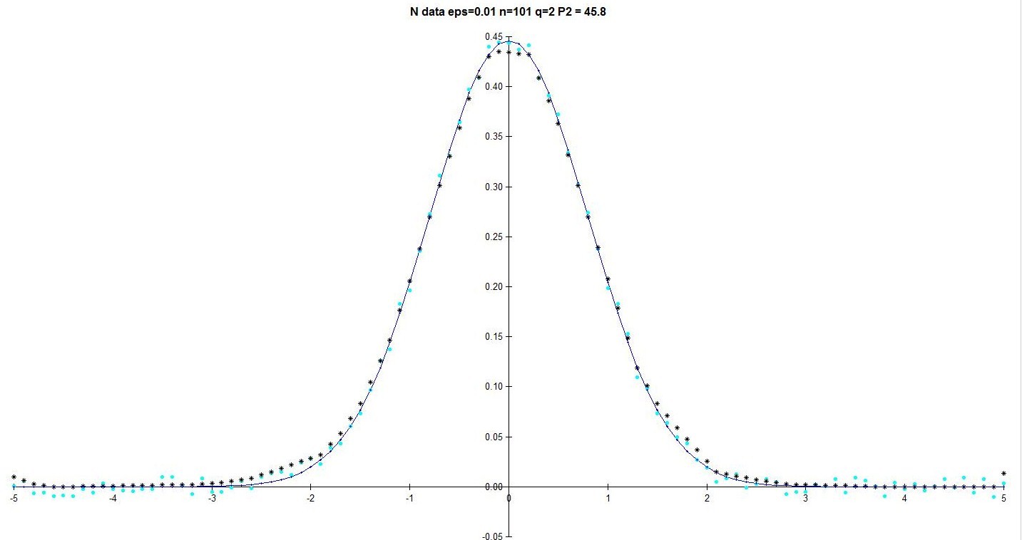
Figure 7: Peaked Data with $n=1$, $q=2$, $\mbox{$\epsilon$}=0.01$, $\mbox{$P_{2}$}=45.8$

The method is very economical, and can give very good results, particularly when the data are close together. Thus it seems a good candidate for large densely packed data, even when the errors are relatively large. BIBLIOGRAPHY

References

• [1] Cullinan, M. P. 1986 Data smoothing by adjustment of divided differences. Ph.D. dissertation, University of Cambridge.
• [2]
• [3] Cullinan, M. P. 1990 Data smoothing using non-negative divided differences and $\ell_{2}$ approximation. IMAJNA 10, pp. 583–608.
• [4]
• [5] Cullinan, M. P. & Powell, M. J. D. 1982 Data smoothing by divided differences. In: Numerical Analysis Proc. Dundee 1981 (G. A. Watson, Ed.). LNIM 912, Berlin: Springer-Verlag, pp.26–37.
• [6]
• [7] Demetriou, I. C. 2002 Signs of divided differences yield least squares data fitting with constrained monotonicity or convexity. Journal of Computational and Applied Mathematics 146.2, pp. 179–211.
• [8]
• [9] Graham, R. L. 1972 An efficient algorithm for determining the convex hull of a finite point set. Inform. Proc. Lett. 1, pp. 132–133.
• [10]
• [11] Hildebrand, F. B. 1956 Introduction to Numerical Analysis. New York: McGraw Hill.
• [12]
• [13] Kruskal, J. B. 1964 Non-metric multidimensional scaling: a numerical method. Psychometrika 29, pp. 115–129.
• [14]
• [15] Miles, R. E. 1959 The complete amalgamation into blocks, by weighted means, of a finite set of real numbers. Biometrika 46, pp. 317–327.
• [16]
• [17] Ubhaya, V. A. 1977 An $O(n)$ algorithm for discrete $n$-point convex approximation with applications to continuous case. Technical Memorandum No. 434 (Operations Research Department, Case Western Reserve University, Cleveland, Ohio 44106, U.S.A.).