Energy spectrum of graphene multilayers in a parallel magnetic field

Abstract

We study the orbital effect of a strong magnetic field parallel to the layers on the energy spectrum of the Bernal-stacked graphene bilayer and multilayers, including graphite. We consider the minimal model with the electron tunneling between the nearest sites in the plane and out of the plane. Using the semiclassical analytical approximation and exact numerical diagonalization, we find that the energy spectrum consists of two domains. In the low- and high-energy domains, the semiclassical electron orbits are closed and open, so the spectra are discrete and continuous, correspondingly. The discrete energy levels are the analogs of the Landau levels for the parallel magnetic field. They can be detected experimentally using electron tunneling and optical spectroscopy. In both domains, the electron wave functions are localized on a finite number of graphene layers, so the results can be applied to graphene multilayers of a finite thickness.

I Introduction

Graphene monolayers have attracted much attention recently because of the unusual Dirac spectrum of electrons Novoselov-2004 . A remarkable manifestation of the Dirac dispersion is the unusual spectrum of the Landau levels in a perpendicular magnetic field, resulting in the anomalous quantum Hall effect (QHE) Novoselov-2005 ; Zhang ; Sadowski ; Gusynin ; Jiang . These results stimulated further investigations of the QHE in the derivatives of graphene. The unusual Landau levels and the QHE were obtained for a graphene bilayer in Ref. McCann . Although the Landau levels in graphite were investigated a long time ago Inoue ; Dresselhaus ; Brandt , recent studies Eva ; Plochocka ; Orlita ; Chuang ; Garcia ; Koshino of graphene multilayers with a moderate number of layers found interesting features in the Landau spectrum. Namely, the spectrum consists of the two families of levels, whose energies scale as $B$ and $\sqrt{B}$, thus indicating the presence of both massive and massless Dirac fermions in the system Eva . The Landau levels for different stacking orders of graphene multilayers were studied in Ref. Guinea .

On the other hand, much less attention was paid to the orbital effect of a magnetic field parallel to the graphene layers. The Shubnikov-de Haas oscillations were extensively studied in graphite in a tilted magnetic field Brandt , but they tend to disappear when the field is parallel to the layers. Ref. Kopelevich studied the influence of a parallel magnetic field on the putative ferromagnetic, superconducting, and metal-insulator transitions in graphite. In Ref. Iye , the angular magnetoresistance oscillations (AMRO) were observed in the stage 2 intercalated graphite (in addition to the Shubnikov-de Haas oscillations) for magnetic fields close to the parallel orientation. AMRO were first discovered in layered organic conductors Kartsovnik88 ; Kajita89 and subsequently observed in many other layered materials: see, e.g., Ref. Cooper and references therein. Motivated by the experiment Iye , a theoretical study of AMRO in graphene multilayers was the original goal of the present paper, with the focus on the peculiarities due to the presence of two sublattice, Dirac spectrum, etc. However, in the standard theory of AMRO Cooper , the interlayer tunneling amplitude is treated as a small perturbation. It is a reasonable approximation for the intercalated graphite Dresselhaus-2002 , but not for the pristine graphite, where it is generally accepted that the interlayer tunneling amplitude is quite large. A non-perturbative treatment of the interlayer tunneling in a tilted magnetic field for graphene multilayers is a very complicated problem. So, we decided to focus first on the simpler case of the parallel magnetic field.

Additional motivation for this work comes from the recent experiment Latyshev-2010 , where the current-voltage $I$-$V$ relation was studied for the current perpendicular to the layers in a mesoscopic graphite mesa consisting of about 20–30 graphene layers. The experimental technique is similar to the previous work on the cuprate superconductors Krasnov and the charge-density-wave materials Latyshev-2005 . When a strong parallel magnetic field up to 55 T is applied to the graphite mesa, the $dI/dV$ curve develops a peak at a non-zero, magnetic-field-dependent voltage $V$ of the order $80$ mV. The appearance of the peak may indicate formation of the Landau levels in the parallel magnetic field, but detailed interpretation of the experimental results is currently unclear.

In this paper, we calculate the electron spectrum of two or many coupled graphene layers in a strong parallel magnetic field. To simplify the problem, we consider only the minimal model with the electron tunneling amplitudes between the nearest sites in the plane ($\gamma_{0}$) and out of the plane ($\gamma_{1}$). The effect of the higher-order tunneling amplitudes Gruneis is briefly discussed in Appendix A. Our results should be valid for the energies greater than the energies of the neglected higher-order tunneling amplitudes and can be verified by tunneling or optical spectroscopy. We focus only on the orbital effect of the magnetic field and disregard possible spin effects Hwang . We find some mathematical similarities between the electron spectrum of graphene multilayers in a parallel magnetic field and that of quasi-one-dimensional Yakovenko ; Goan and quasi-two-dimensional Lebed organic conductors Lebed-book .

We start with the analysis of a graphene bilayer in a parallel magnetic field (Sec. II) and then proceed to the infinite number of layers (Sec. III). We investigate both the quasiclassical electron orbits in momentum space (Sec. III.2.1) and the exact equation for the energy eigenfunctions, which reduces to the Mathieu equation (Sec. III.2.2). We employ both the analytical WKB method and exact numerical diagonalization to find the energy eigenvalues and eigenfunctions. We identify the low-energy domain characterized by closed orbits and discrete spectrum (Sec. III.2.3) and the high-energy domain with open orbits and continuous spectrum (Sec. III.2.4). The case of a finite number of layers is analyzed at the end of Sec. III.2.3. The effect of the tunneling amplitude $\gamma_{3}$ responsible for trigonal warping is discussed in Appendix A.

II Graphene bilayer

II.1 Model

First, we consider a graphene bilayer and then generalize the problem to many layers. The crystal lattice of the Bernal-stacked graphene bilayer is shown in Fig. 1. The distance between the nearest atoms in graphene is $a=1.4$ Å, and the distance between the layers is $d=3.3$ Å. We restrict our analysis to the minimal tight-binding model Koshino with the intra- and inter-layer tunneling amplitudes $\gamma_{0}=3.16$ eV and $\gamma_{1}=0.38$ eV.

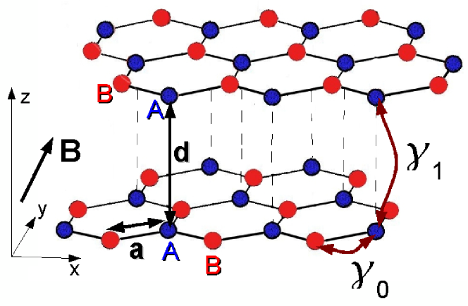
Figure 1: (Color online) A pair of Bernal-stacked graphene layers in the parallel magnetic field $\bm{B}$ applied along the $y$ direction. $\gamma_{0}$ and $\gamma_{1}$ are the electron tunneling amplitudes.

There are two sublattices on each graphene layer. Thus, the electron wave function is the vector

$$\Psi=(\psi_{1}^{A},\psi_{1}^{B},\psi_{2}^{A},\psi_{2}^{B}),$$ (1)

where the subscripts 1 and 2 enumerate the layers, and the superscripts $A$ and $B$ denote sublattices on each layer. Sublattices can be selected in various ways. It is convenient for us to assign the atoms connected by the interlayer tunneling $\gamma_{1}$ in the Bernal stack to sublattice A and other atoms to sublattice B, as shown in Fig. 1.

In the vicinity of the K point in the Brillouin zone, the electron Hamiltonian has the form

$$H=\left(\begin{array}[]{cc}v_{F}(\bm{p}\cdot\bm{\sigma})&\gamma_{1}I^{A}\\ \gamma_{1}I^{A}&v_{F}(\bm{p}\cdot\bm{\sigma}^{\ast})\\ \end{array}\right).$$ (2)

Hamiltonian (2) acts on the vector (1). Correspondingly, $\bm{\sigma}=(\sigma_{x},\sigma_{y})$ are the Pauli matrices acting in the sublattice space; $\bm{p}=p_{x}\hat{\bm{x}}+p_{y}\hat{\bm{y}}$ is the in-plane momentum measured from the K point; $v_{F}=(3/2\hbar)\gamma_{0}a\approx 10^{8}$ cm/s is the electron velocity in graphene. The terms $v_{F}(\bm{p}\cdot\bm{\sigma})$ and $v_{F}(\bm{p}\cdot\bm{\sigma}^{\ast})$ describe the in-plane Hamiltonians of the graphene layers. Our choice of the A and B sublattices results in the diagonal elements having both $\bm{\sigma}$ and $\bm{\sigma}^{\ast}$ (complex-conjugated) terms. The term $\gamma_{1}I^{A}$ represents the interlayer tunneling, where the matrix

$$I^{A}=\frac{1}{2}(I+\sigma_{z})=\left(\begin{array}[]{cc}1&0\\ 0&0\\ \end{array}\right)$$ (3)

connects sublattices A of the adjacent graphene layers.

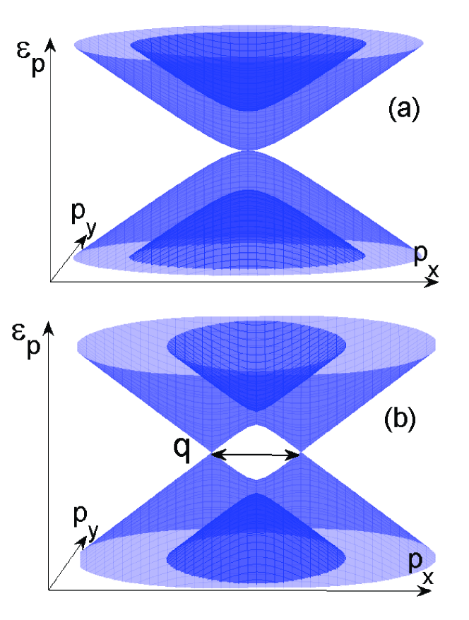
Figure 2: (Color online) (a) The electron spectrum (4) of a graphene bilayer in zero magnetic field. (b) The spectrum (12) in a nonzero parallel magnetic field. The magnetic field splits the parabolic spectrum into the two Dirac cones. An exaggerated value $q=5$ of the magnetic field parameter was utilized here.

Hamiltonian (2) has four eigenvalues

$$\varepsilon(\bm{p})=\pm\frac{\gamma_{1}}{2}\pm\sqrt{\frac{\gamma_{1}^{2}}{4}+v_{F}^{2}p^{2}}.$$ (4)

The well-known spectrum (4) is shown in Fig. 2(a). The spectrum consists of the four bands with the parabolic dispersion for small $p$.

II.2 Parallel magnetic field

Now let us introduce the in-plane magnetic field $\bm{B}=\hat{\bm{y}}B$ applied along the $y$ axis. We choose the gauge $\bm{A}=\hat{\bm{x}}Bz$ and use the Peierls substitution

$$\bm{p}\rightarrow\bm{p}+\frac{e}{c}\bm{A}.$$ (5)

Here, we took into account the negative sign of the electron charge, so $e$ corresponds to its absolute value. If the layer number is denoted by $j$, the in-plane electron momentum on the $j$-th layer changes to

$$\bm{p}_{j}=\bm{p}+j\,\Delta p\,\hat{\bm{x}},$$ (6)

where $\Delta{p}$ is

$$\Delta{p}=\frac{e}{c}Bd,\qquad\frac{\Delta{p}}{\hbar B}=5\times 10^{3}\,\rm{cm^{-1}\,T^{-1}}.$$ (7)

The momentum change $\Delta p$ has the following physical meaning. When an electron tunnels between the layers, the Lorentz force $\bm{F}=-\frac{e}{c}[\bm{v}\times\bm{B}]$ changes the in-plane momentum by

$$\Delta p_{x}=\int F_{x}dt=\frac{e}{c}B_{y}\int v_{z}\,dt=\frac{e}{c}Bd.$$ (8)

The change in the in-plane momentum results in the relative shift of the Dirac points on the different layers in the momentum space.

To simplify equations in the rest of the paper, it is convenient to switch to the dimensionless variables

$$\frac{v_{F}\bm{p}}{\gamma_{1}}\to\bm{p},\quad\frac{v_{F}\Delta p}{\gamma_{1}}\to q,\quad\frac{\varepsilon}{\gamma_{1}}\to\varepsilon.$$ (9)

Here the parameter $q$ is the dimensionless ratio of the “magnetic shift” $v_{F}\Delta p$ and the interlayer tunneling amplitude $\gamma_{1}$

$$q=\frac{v_{F}\Delta p}{\gamma_{1}}=\frac{v_{F}}{\gamma_{1}}\left(\frac{e}{c}Bd\right)=0.88\times 10^{-3}B[\rm{T}].$$ (10)

The parameter $q$ describes the orbital effect of the magnetic field in our model and will be frequently referred to as the magnetic field for shortness. It is worth noting that even for a strong magnetic field this parameter is small $q\ll 1$, e.g., $q=0.044$ for $B=50$ T.

Applying the Peierls substitution (6) to Hamiltonian (2) and switching to the dimensionless variables (9), we obtain

$$H=\left(\begin{array}[]{cc}((\bm{p}-\bm{q})\cdot\bm{\sigma})&I^{A}\\ I^{A}&(\bm{p}\cdot\bm{\sigma}^{\ast})\\ \end{array}\right).$$ (11)

Hamiltonian (11) has the following spectrum:

$$\varepsilon(\bm{p})=\pm{\frac{1}{\sqrt{2}}\sqrt{\bm{p}^{2}+(\bm{p}-\bm{q})^{2}+1\pm W}},$$ (12)

where

$$W=\sqrt{\left[(\bm{p}-\bm{q})^{2}-\bm{p}^{2}\right]^{2}+2\bm{p}^{2}+2(\bm{p}-\bm{q})^{2}+1}.$$ (13)

In contrast to the parabolic dispersion (4), the spectrum (12) has two Dirac points separated by the magnetic shift $q$ with a saddle point in between, as shown in Fig. 2(b). Expanding Eq. (12) around one of the Dirac points

$$\varepsilon(\bm{p})\approx\pm\frac{q}{\sqrt{1+q^{2}}}\,p,$$ (14)

we find that the slope of the Dirac cones is controlled by the magnetic field and is greatly reduced for $q\ll 1$.

A dispersion similar to Eq. (12) was found for the twisted graphene layers in Ref. Santos , where the relative displacement of the two Dirac cones in the momentum space results from the spatial rotation of the layers

$$\Delta p_{\rm{rot}}/\hbar=K_{0}\Delta\phi=6\times 10^{6}\,\rm{cm^{-1}}.$$ (15)

Here $\Delta\phi=2^{\circ}$ is the twist angle, and $K_{0}=4\pi/3\sqrt{3}a$ is the distance between the $\Gamma$ and K points in the reciprocal space. The saddle point between the two Dirac points results in the Van Hove singularity in the density of states, which was observed experimentally in electron tunneling in Ref. Eva1 . Comparing Eq. (7) with Eq. (15), we observe that the magnetic field effect is much weaker than the effect of twisting. Even for $B=50$ T, the magnetic shift is $\Delta p/\hbar=2.5\times 10^{5}\,\rm{cm^{-1}}$ is much smaller than the rotational shift $\Delta p_{\rm{rot}}/\hbar$.

III Graphite

III.1 Model

Now we proceed to the discussion of graphene multilayers. First we solve the problem for an infinite number of layers, i.e., for graphite, and then briefly mention the effect of a finite number of layers.

By analogy with the bilayer Hamiltonian (2), the Hamiltonian of graphite without magnetic field reads in the adopted units (9)

$$H=\left(\begin{array}[]{ccccc}\ddots&&&&\\ &(\bm{p}\cdot\bm{\sigma})&I^{A}&&\\ &I^{A}&(\bm{p}\cdot\bm{\sigma}^{\ast})&I^{A}&\\ &&I^{A}&(\bm{p}\cdot\bm{\sigma})&\\ &&&&\ddots\\ \end{array}\right).$$ (16)

It acts on the vector

$$\Psi=(\cdots\,\tilde{\psi}_{j-1}\,\tilde{\psi}_{j}\,\tilde{\psi}_{j+1}\cdots),\qquad\tilde{\psi}_{j}=(\psi_{j}^{A}\,\psi_{j}^{B}),$$ (17)

where the subscript $j$ denotes the layer number, and the superscripts $A$ and $B$ denote sublattices.

Using the momentum representation in the $z$ direction and introducing the corresponding momentum $k$ (in addition to the in-plane momentum $\bm{p}$), we transform Hamiltonian (16) into a $4\times 4$ matrix similar to the graphene bilayer Hamiltonian (2)

$$H=\left(\begin{array}[]{cc}(\bm{p}\cdot\bm{\sigma})&2I^{A}\cos k\\ 2I^{A}\cos k&(\bm{p}\cdot\bm{\sigma}^{\ast})\\ \end{array}\right).$$ (18)

Hamiltonian (18) has the following spectrum

$$\varepsilon_{1,2}(\bm{p},k) = \pm\cos k+\sqrt{\cos^{2}k+p^{2}},$$ (19)

$$\varepsilon_{3,4}(\bm{p},k) = \pm\cos k-\sqrt{\cos^{2}k+p^{2}}.$$ (20)

The subscripts (1,2) and (3,4) denote positive and negative energies, whereas the subscripts (1,3) and (2,4) correspond to the terms $\pm\cos k$. Because the spectrum has the electron-hole symmetry, we consider only the positive energies $\varepsilon_{1,2}$. The branches 1 and 2 are equivalent, in the sense that $\varepsilon_{1}(\bm{p},k+\pi)=\varepsilon_{2}(\bm{p},k)$. Thus, it is sufficient to consider only one branch $\varepsilon_{1}$, which is plotted in Fig. 3. Since the off-diagonal elements of Hamiltonian (18) vanish for $k=\pi/2$, the dispersion has the Dirac-type form $\varepsilon_{1}(\bm{p},\pi/2)=p$ for $k=\pi/2$, as shown in Fig. 3.

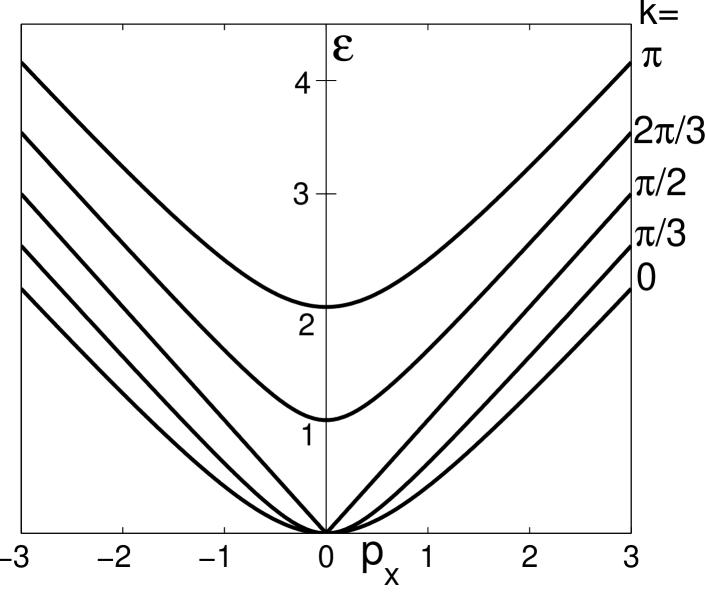
Figure 3: Spectrum $\varepsilon_{1}(\bm{p},k)$ (19) of Hamiltonian (18) for $p_{y}=0$. Each curve corresponds to a given value of the out-of-plane momentum $k$ indicated on the right. The axes are given in the adopted dimensionless units (9).

.

III.2 Parallel magnetic field

III.2.1 Semiclassical analysis

In the presence of a magnetic field, electrons move along the isoenergetic surfaces in the momentum space. For the field $\bm{B}=\hat{\bm{y}}B$ along the $y$ direction, the electron orbits lie on the intersections of the isoenergetic surfaces of the dispersion (19) and the planes parallel to the $(p_{x},k)$ plane. The cross-sections of the isoenergetic surfaces $\varepsilon_{1}(\bm{p},k)=\varepsilon=\rm{const}$ with the $(p_{x},k)$ plane at $p_{y}=0$ are shown in Fig. 4. The arrows indicate the direction of electron motion.

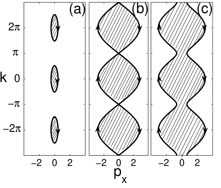
Figure 4: Semiclassical electron orbits in the momentum space for the in-plane magnetic field along the $y$ axis. Only the orbits with $p_{y}=0$ are shown. They are obtained by intersecting the $(p_{x},k)$ plane with the isoenergetic surfaces $\varepsilon_{1}(\bm{p},k)=\varepsilon$ for (a) $\varepsilon=0.1$, (b) $\varepsilon=2$, (c) $\varepsilon=2.2$. The orbits are (a) closed for $|\varepsilon|<2$ and (c) open for $|\varepsilon|>2$.

Topology of the electron orbits changes with the increase of the energy $\varepsilon$. The isoenergetic surfaces for the dispersion (19) are closed for $0<\varepsilon<2$, so the orbits are closed too, see Fig. 4(a). Thus, based on the Onsager quantization rule Onsager , the spectrum is discrete for this energy interval. However, at the critical energy $\varepsilon=2$, the isoenergetic surfaces reconnect, as shown in Fig. 4(b), and become open for $\varepsilon>2$, resulting in the open orbits shown in Fig. 4(c). Open semiclassical orbits lead to a continuous energy spectrum.

Fig. 4 shows only the electron orbits for $p_{y}=0$ and $\varepsilon>0$. We can find the topology of the electron orbits and the character of the spectrum for an arbitrary $p_{y}$, which is a good quantum number for the magnetic field along the $y$ direction. The orbits are open, so the spectrum is continuous in $p_{x}$ for

$$\varepsilon^{2}-2|\varepsilon|>p_{y}^{2}.$$ (21)

The orbits are closed, so the spectrum is discrete and degenerate in $p_{x}$ for

$$\varepsilon^{2}-2|\varepsilon|<p_{y}^{2}<\varepsilon^{2}+2|\varepsilon|.$$ (22)

There are no orbits and no states for

$$p_{y}^{2}>\varepsilon^{2}+2|\varepsilon|.$$ (23)

The domains of the continuous and discrete spectra, defined by the inequalities (21), (22), and (23), are shown in Fig. 5 in the $(p_{y},\varepsilon)$ plane.

III.2.2 Mathieu equation

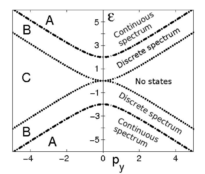
Figure 5: Domains of the continuous and discrete spectra in the ($p_{y},\varepsilon$) plane. The dashed-dotted and dotted curves represent solutions of the equations $\varepsilon^{2}-2|\varepsilon|=p_{y}^{2}$ and $\varepsilon^{2}+2|\varepsilon|=p_{y}^{2}$. The spectrum is continuous in the region A defined by Eq. (21), discrete in the region B defined by Eq. (22), and there are no states in the region C defined by Eq. (23).

Now we present a more formal and exact analysis of the electron spectrum in a parallel magnetic field. Applying the Peierls substitution (6) in the dimensionless units

$$\bm{p}_{j}=\bm{p}+j\bm{q},\qquad\bm{q}=\hat{\bm{x}}q$$ (24)

to Hamiltonian (16), we obtain

$$H=\left(\begin{array}[]{ccccc}\ddots&&&&\\ &(\bm{p_{j-1}}\cdot\bm{\sigma})&I^{A}&&\\ &I^{A}&(\bm{p}_{j}\cdot\bm{\sigma}^{\ast})&I^{A}&\\ &&I^{A}&(\bm{p}_{j+1}\cdot\bm{\sigma})&\\ &&&&\ddots\\ \end{array}\right).$$ (25)

The eigenvalue problem $H\Psi=\varepsilon\Psi$ for $H$ (25) and $\Psi$ (17) reads in components

$$I^{A}(\tilde{\psi}_{j-1}+\tilde{\psi}_{j+1})+\left[\bm{\sigma}^{(\ast)}\cdot(\bm{p}+j\bm{q})-\varepsilon\right]\tilde{\psi}_{j}=0.$$ (26)

Here, $\bm{\sigma}^{(\ast)}$ denotes $\bm{\sigma}$ for even j and $\bm{\sigma}^{\ast}$ for odd j. The matrix equation (26) represents a set of two equations. One of them relates $\psi_{j}^{B}$ and $\psi_{j}^{A}$ on the same layer and has the simple form

$$\psi_{j}^{B}=\frac{p_{x}\pm ip_{y}+jq}{\varepsilon}\psi_{j}^{A},$$ (27)

where the signs $\pm$ correspond to even and odd $j$. Using Eq. (27), we algebraically eliminate $\psi_{j}^{B}$ components in Eq. (26) and reduce it to the simpler equation

$$\psi^{A}_{j+1}+\psi^{A}_{j-1}=\left(\varepsilon-\frac{(\bm{p}+j\bm{q})^{2}}{\varepsilon}\right)\psi^{A}_{j},$$ (28)

which has the same form for even and odd $j$. From now on we drop the superscripts A. In the Fourier representation

$$\psi_{j}=\int_{0}^{2\pi}\psi(k)\,e^{ikj}dk,$$ (29)

Eq. (28) becomes

$$\left(\frac{d}{dk}-i\frac{p_{x}}{q}\right)^{2}\psi(k)-V(k)\,\psi(k)=0,$$ (30)

where

$$V(k)=\frac{2\varepsilon}{q^{2}}\cos k-\frac{\varepsilon^{2}-p_{y}^{2}}{q^{2}}.$$ (31)

Here, $\psi(k)$ is a $2\pi$-periodic, twice-differentiable function $\psi(k)=\psi(k+2\pi)$. To further simplify Eq. (30), we introduce the function $\phi(k)$

$$\psi(k)=e^{ik(p_{x}/q)}\phi(k),$$ (32)

which eliminates the term $ip_{x}/q$ from Eq. (30) and reduces it to the angular Mathieu equation for $\phi(k)$

$$\frac{d^{2}\phi(k)}{dk^{2}}-V(k)\phi(k)=0.$$ (33)

Eq. (33) is equivalent to the Schrödinger equation for a particle moving in the 1D potential $V(k)$ (31). The variables $\varepsilon$ and $p_{y}$ are the parameters that control $V(k)$.

Since $V(k)$ is periodic in $k$, the Bloch theorem can be applied, so the solutions of Eq. (33) have the form

$$\phi_{\kappa}(k)=e^{ik\kappa}u_{\kappa}(k).$$ (34)

Here, $\kappa$ is the quasimomentum in the space reciprocal to the $k$ space, and $u_{\kappa}(k)$ is a $2\pi$-periodic function in $k$. From Eqs. (32) and (34) and the periodicity requirement for $\psi(k)$, we select the solutions of Eq. (33) with $\kappa=-p_{x}/q$. Since the solutions of Eq. (33) are periodic in the quasimomentum $\phi_{\kappa+1}(k)=\phi_{\kappa}(k)$, the parameter $\varepsilon$ in Eq. (30) must be periodic in $p_{x}$: $\varepsilon(p_{x})=\varepsilon(p_{x}+q)$. Therefore, the magnetic field effectively introduces the magnetic Brillouin zone in $p_{x}$ with the period $q$.

We have reduced the original eigenvalue problem (28) to the convenient differential equation (33). Different regimes for its solutions are controlled by the parameters $p_{y}$ and $\varepsilon$. If the criterion (22) is satisfied, the 1D classical motion is bounded by the barriers of $V(k)$, as shown in Fig. 6(a) for $\varepsilon=0.1$ and $p_{y}=0$. Then the energy spectrum is discrete. On the other hand, if the criterion (21) is satisfied, the potential is negative $V(k)<0$ for any $k$, as shown in Fig. 6(b) for $\varepsilon=2.1$ and $p_{y}=0$. Then the motion of a particle is unbounded, and the spectrum is continuous in $p_{x}$. The first regime corresponds to the closed orbits in Fig. 4(a), and the second regime to the open orbits in Fig. 4(c). In the following sections, we use the approaches of both Sec. III.2.1 and this section to obtain and interpret the results.

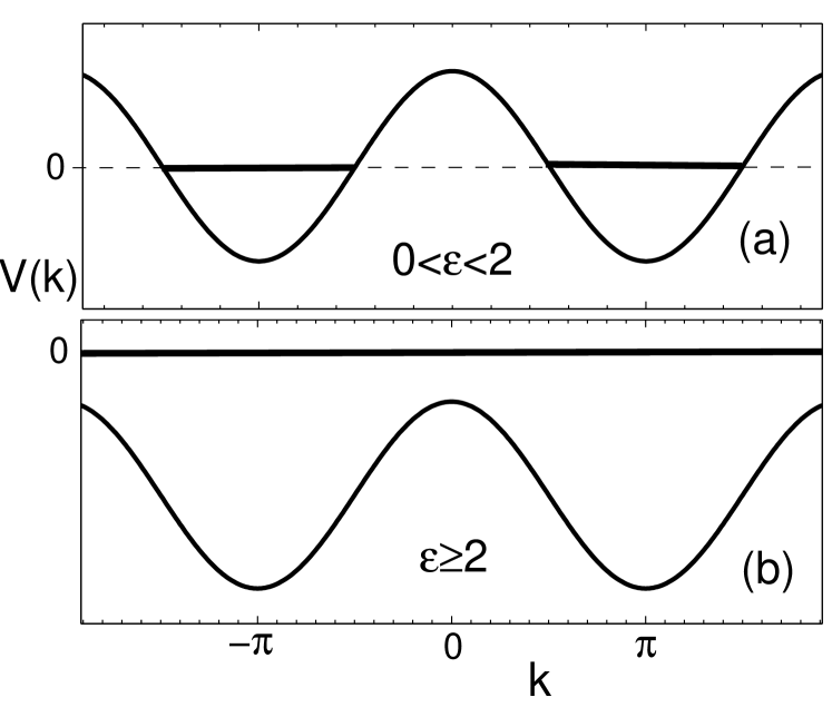
Figure 6: The plots of $V(k)$ (31) for $p_{y}=0$. The cases of $\varepsilon=0.1$ and $\varepsilon=2.1$ are shown on the panels (a) and (b). The classically permitted region corresponds to $V(k)<0$, as indicated by the thick horizontal line. Thus, the panels (a) and (b) represent bounded and unbounded motion.

III.2.3 Closed orbits

In this section, we study the electron spectrum in the domain of the ($p_{y},\varepsilon$) plane defined by the criterion (22) and labeled by the letter B in Fig. 5. In this case, the classical motion of a particle in the 1D potential (31) is restricted to the potential wells separated by the barriers, as shown in Fig. 6(a). The height of the barriers is

$$h(p_{y},\varepsilon)={\rm max}[V(k)]=\frac{\varepsilon(2-\varepsilon)+p_{y}^{2}}{q^{2}}.$$ (35)

The barriers $h(p_{y},\varepsilon)\gg 1$ are high everywhere, except at the boundary of the domain (22). Thus, we can neglect tunneling and use the WKB quantization rule for a single well of $V(k)$

$$4\int\limits_{\arccos{a}}^{\pi}\sqrt{-2\varepsilon\cos k+\varepsilon^{2}-p_{y}^{2}}\,dk=2\pi\left(n+\frac{1}{2}\right)q,$$ (36)

where

$$a=\frac{\varepsilon^{2}-p_{y}^{2}}{2\varepsilon}.$$ (37)

The integral on the left-hand side of Eq. (36) is proportional to the area enclosed by the electron orbit in momentum space, see Fig. 4(a). Thus, Eq. (36) is equivalent to the Onsager quantization rule in a magnetic field Onsager . Using the incomplete elliptic function of the second kind

$$E(\phi,m)=\int_{0}^{\phi}\sqrt{1-m^{2}\sin^{2}\alpha}\,d\alpha,$$ (38)

Eq. (36) can be written as

$$8\sqrt{2\varepsilon}\sqrt{1+a}\,E\left(\frac{\pi+2\arcsin a}{4},\sqrt{\frac{2}{1+a}}\right)$$

$$=2\pi\left(n+\frac{1}{2}\right)q.$$ (39)

Eqs. (39) and (37) implicitly define $\varepsilon_{n}(p_{x},p_{y})$ as a function of $p_{y}$ and $n$ for a given magnetic field $q$, and the spectrum is degenerate in $p_{x}$.

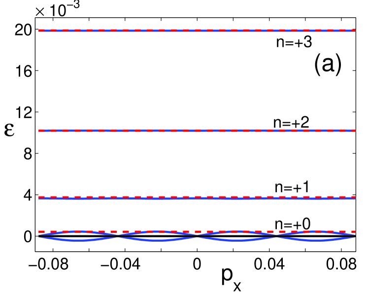
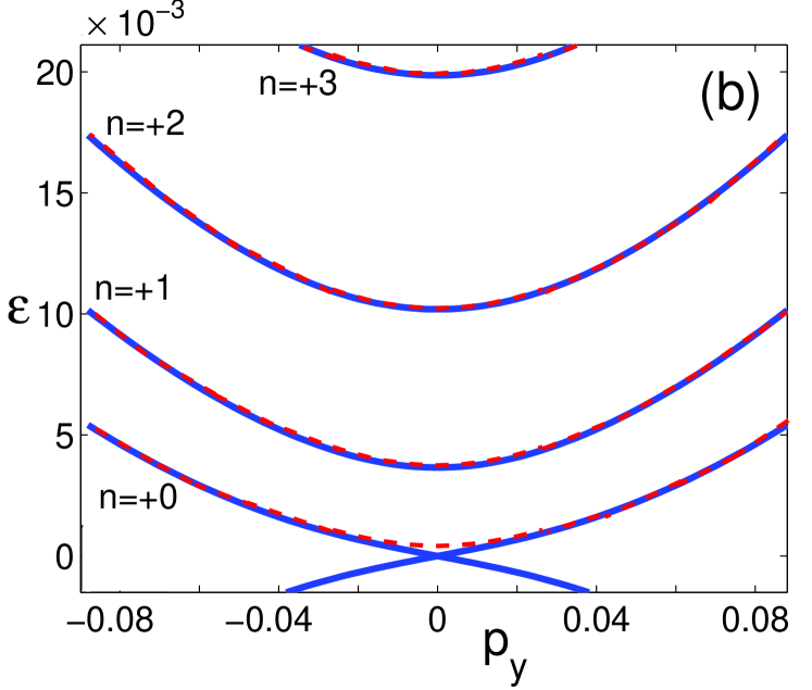
Figure 7: (Color online) Low-energy levels $\varepsilon_{n}(p_{x},p_{y})$ for $q=0.044$. Panel (a) shows $\varepsilon_{n}(p_{x},0)$ vs $p_{x}$ for $p_{y}=0$, and panel (b) shows $\varepsilon_{n}(0,p_{y})$ vs $p_{y}$ for $p_{x}=0$. Solid lines represent exact numerical diagonalization of Hamiltonian (25). Dashed lines represent the WKB analytical approximation (39). All quantities are presented in the adopted dimensionless units (9).

To check validity of the WKB approximation, we diagonalize of the original Hamiltonian (25) numerically and compare results with the solutions of Eq. (39). Momentum dependences of $\varepsilon_{n}(p_{x},0)$ and $\varepsilon_{n}(0,p_{y})$ are shown in Figs. 7(a) and (b) for a few lowest energy levels at $q=0.044$. The analytical approximation (39) agrees well with the numerical results for $n\neq 0$. The discrete energy levels shown in Fig. 7(a) are degenerate in $p_{x}$ and represent the Landau levels in a parallel magnetic field. However, the $n=0$ level has a remarkable dispersion in $p_{x}$. Similarly to the spectrum of the graphene bilayer in Fig. 2(b), the $n=0$ level consists of a series of the Dirac cones shifted by the vector $q$. This dispersion cannot be obtained from the approximate WKB equation (39), because of the divergence at $\varepsilon=0$ in the original equations (27) and (28).

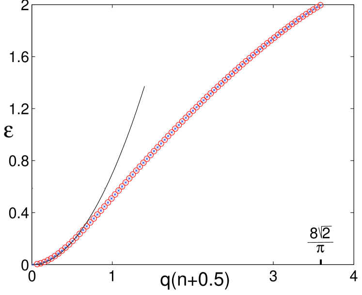
Figure 8: (Color online) Energy levels $\varepsilon_{n}(0,0)$ vs the quantum number $n$ at $p_{x}=0$ and $p_{y}=0$ for $q=0.044$. The horizontal axis shows the combination $q(n+1/2)$. The circles represent solutions of the WKB equation (39), and the small points inside the circles represent numerical data. The quadratic approximation (41) is shown by the solid line. All quantities are presented in the adopted dimensionless units (9).

Fig. 7(b) shows that the energy levels $\varepsilon_{n}(0,p_{y})$ have a quadratic dispersion in $p_{y}$, except for the $n=0$ level. Given the degeneracy in $p_{x}$, the energy levels $\varepsilon_{n}(p_{x},p_{y})$ form one-dimensional bands in $p_{y}$, so the density of states diverges at the bottom points $\varepsilon_{n}(p_{x},0)$ of the bands. These singularities in the density of state can be detected experimentally by electron tunneling or optical spectroscopy. The energies $\varepsilon_{n}(0,0)$ are plotted in Fig. 8 in the interval $0<\varepsilon<2$ vs the combination $q(n+1/2)$ appearing in Eq. (39). Depending on the magnetic field $q$, a different number $n_{\rm{max}}$ of the discrete levels fills the curve. By setting $\varepsilon=2$ in Eq. (36), we obtain

$$n_{\mathrm{max}}+\frac{1}{2}=\frac{8\sqrt{2}}{\pi q}=\frac{3.6}{q}.$$ (40)

For example, for $q=0.044$, we have $n_{\rm{max}}=81$ levels, which are depicted by circles in Fig. 8.

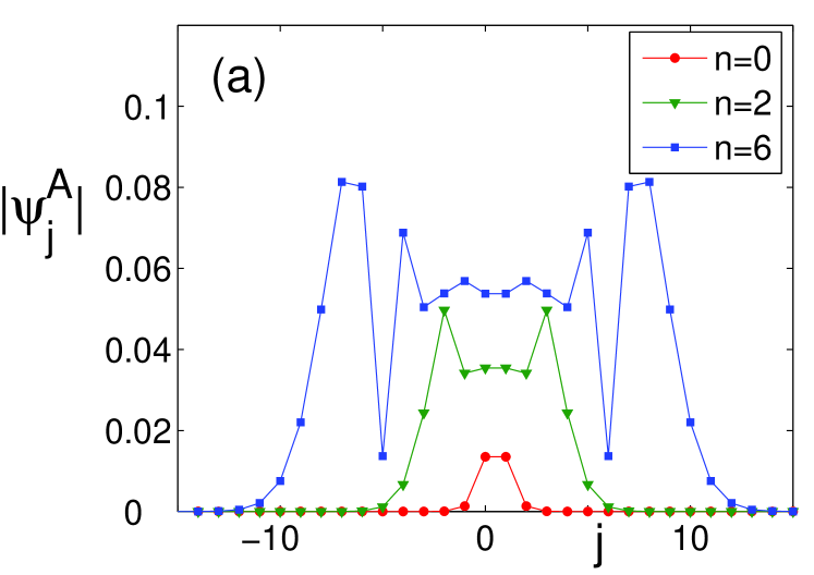
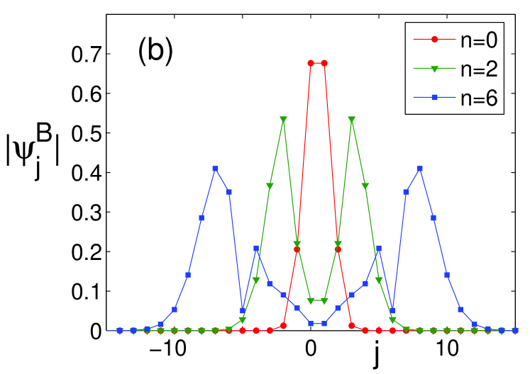
Figure 9: (Color online) The absolute values of the wave functions $|\psi_{j}^{A}|$ and $|\psi_{j}^{B}|$ on the sublattices A and B vs the layer number $j$ for $q=0.044$, $p_{x}=q/2$, and $p_{y}=0$. The variable $n$ denotes the energy level number.

For small $\varepsilon$ and $p_{y}=0$, we find from Eq. (39)

$$\varepsilon_{n}=\frac{\pi^{2}}{32E^{2}\left(\frac{\pi}{4},\sqrt{2}\right)}q^{2}\left(n+\frac{1}{2}\right)^{2}=0.7\,q^{2}\left(n+\frac{1}{2}\right)^{2}.$$ (41)

We observe that the energies (41) depend quadratically on the level number $n$ and the magnetic field $q$. This dependence is different from the usual Landau level dependence, where the energies are linear in the field and in the quantum number. The reason for the unusual dependence in our case is the following. For small $\varepsilon$, the semiclassical orbit in Fig. 4(a) shrinks to a thin ellipsoid of the length $\pi$ in the $k$ direction and the width $\sqrt{2\varepsilon}$ in the $p_{x}$ direction. Thus, the area enclosed by the semiclassical orbit is proportional to $\sqrt{\varepsilon}$, so the Onsager quantization rule gives quadratic dependence of the energy on the magnetic field and the level number $n$. The quadratic approximation (41) is shown by the solid line in Fig. 8 and works well in the region $\varepsilon<0.1$.

Fig. 9 shows the plots of $|\psi_{j}^{A}|$ and $|\psi_{j}^{B}|$ vs the layer number $j$ for several energy levels $n$. We observe that the magnetic field causes localization of the wave function on a finite number of layers. According to Eq. (27), the wave functions for the low energy levels $\varepsilon_{n}$ are localized predominantly on the sublattice B. The magnitudes of $|\psi_{j}^{A}|$ and $|\psi_{j}^{B}|$ are shown by different vertical scales in panels (a) and (b) of Fig. 9.

Now let us briefly discuss the spectrum of a finite system with the total number of layers $N$. Fig. 10 shows $\varepsilon_{n}(p_{x},0)$ for $N=7$, 21, and $\infty$. The degeneracy in $p_{x}$ is lifted for a finite number of layers, but, with increasing $N$, the spectrum approaches to that of the infinite system with $N=\infty$. Indeed, if the localization length for a particular energy level is shorter than the size of the system, the energy of the level is the same as for $N=\infty$. Thus, the results obtained for $N=\infty$ are applicable to a finite system with a sufficient large $N$.

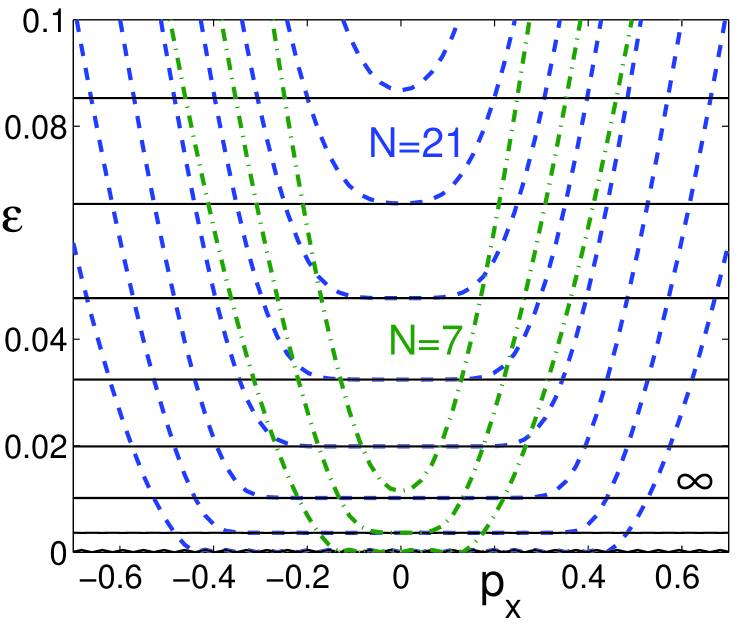
Figure 10: (Color online) Energy spectrum $\varepsilon_{n}(p_{x},0)$ vs $p_{x}$ at $p_{y}=0$ and $q=0.044$ for the system with a finite number of layers $N$. The dashed-dotted, dashed, and solid lines correspond to $N=7$, 21, and $\infty$. All quantities are presented in the adopted dimensionless units (9).

III.2.4 Open orbits

Now we study the energy spectrum in the domain defined by Eq. (21) and labeled by the letter A in Fig. 5. It corresponds to the open electron orbits in Fig. 4(c). In the Mathieu equation (33), the potential $V(k)<0$ is negative for any $k$, so the motion is unbounded, as shown in Fig. 6(b). Then, the WKB solutions of Eq. (33) are

$$\phi(k)=e^{\pm iS(k)},\qquad S(k)=\int_{0}^{k}\sqrt{|V(k)|}\,dk,$$ (42)

where the signs $\pm$ correspond to the direction of motion. Because of the periodicity requirement for $\psi(k)$ and Eq. (32), the phase accumulation in Eq. (42) over the period $2\pi$ must be equal to $-2\pi p_{x}/q$ plus an integer multiple of $2\pi$. Thus we obtain the following quantization condition for the open orbits

$$qS(2\pi)=2\int\limits_{0}^{\pi}\sqrt{-2\varepsilon\cos k+\varepsilon^{2}-p_{y}^{2}}\,dk=\mp 2\pi(p_{x}+\tilde{n}q).$$ (43)

Here the integer $\tilde{n}$ is different from the integer $n$ in Eq. (36) and takes both negative and positive values. The sign of $p_{x}+\tilde{n}q$ corresponds to the two solutions in Eq. (42). Eq. (43) can be represented in terms of the elliptic integral (38)

$$4\sqrt{2\varepsilon}\sqrt{1+a}\,\,E\left(\frac{\pi}{2},\sqrt{\frac{2}{1+a}}\right)=\mp 2\pi(p_{x}+\tilde{n}q),$$ (44)

where the parameter $a$ is given by Eq. (37). In contrast to Eq. (39), Eq. (44) contains $p_{x}$, so the energy levels $\varepsilon_{n}(p_{x},p_{y})$ continuously depend on $p_{x}$.

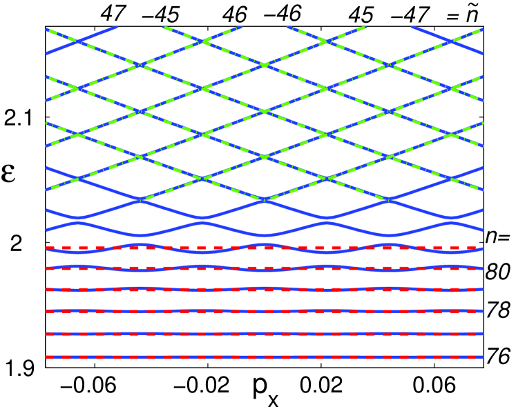
Figure 11: (Color online) Energy spectrum around $\varepsilon=2$ for $q=0.044$ and $p_{y}=0$. The solid lines are obtained by numerical diagonalization of Hamiltonian (25). The dashed lines, obtained from Eq. (39), are labeled by the integer $n$ shown on the right. The dashed-dotted lines, obtained from Eq. (44), are labeled by the integer $\tilde{n}$ shown at the top. This plot illustrates a transition from discrete to continuous spectrum. All quantities are presented in the dimensionless units (9).

The energy spectra obtained from Eqs. (39) and (44) are compared in Fig. 11 with the results of numerical diagonalization of Hamiltonian (25) around the critical energy $\varepsilon=2$ for $p_{y}=0$. For $\varepsilon<2$, the spectrum consists of the energy levels degenerate in $p_{x}$, which are well described by the analytical approximation (39) for closed orbits. The corresponding level number $n$ is shown on the right in Fig. 11. At the energy $\varepsilon=2$, the spectrum undergoes a transition to the regime of continuous dispersion in $p_{x}$. For $\varepsilon>2$, the spectrum consists of the two families of lines with the opposite slopes. This spectrum is well described by the analytical approximation (44) for open orbits. The corresponding number $\tilde{n}$ labels the dispersion lines and takes both positive and negative values shown at the top in Fig. 11. Because the left-hand sides of Eqs. (39) and (44) differ by the factor of 2 at $\varepsilon=2$ and $p_{x}=0$, the numbers $n$ and $\tilde{n}$ are connected as $n\approx 2|\tilde{n}|$. The approximations (39) and (44) stop working in the vicinity of the critical energy $\varepsilon=2$.

For a high energy $\varepsilon$, when the parameter $a$ (37) is large, we can obtain the spectrum explicitly by expanding the square root in Eq. (42) for $S(k)$ in powers of $1/a$

$$S(k)=\frac{\sqrt{\varepsilon^{2}-p_{y}^{2}}}{q}k-\frac{\varepsilon\sin k}{q\sqrt{\varepsilon^{2}-p_{y}^{2}}}.$$ (45)

Then the quantization condition (43) gives

$$\sqrt{\varepsilon^{2}-p_{y}^{2}}=\mp(p_{x}+\tilde{n}q),$$ (46)

which can be written as

$$\varepsilon_{\tilde{n}}^{2}=(p_{x}+\tilde{n}q)^{2}+p_{y}^{2}.$$ (47)

The spectrum Eq. (47) is the same as for decoupled graphene layers with the Peierls substitution (24).

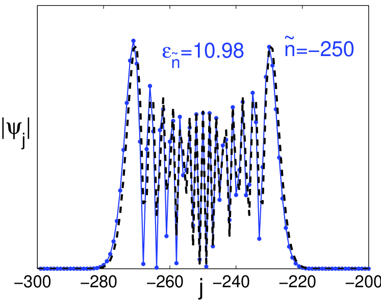
Figure 12: (Color online) The absolute value of the wave function $|\psi_{j}|$ vs the layer number $j$ for a state from the domain of continuous spectrum. The parameters of the plot are $\tilde{n}=-250$, $\varepsilon_{\tilde{n}}=10.98$, $p_{x}=p_{y}=0$, and $q=0.044$. The solid and dashed lines represent exact numerical diagonalization of Hamiltonian (25) and the approximate analytical formula (50), respectively.

Substituting the square root expression from Eq. (46) into Eq. (45), we obtain the approximate WKB wave functions (42) for $\varepsilon>0$

$$\phi(k)=\exp\left(-i\frac{p_{x}+\tilde{n}q}{q}k+i\frac{\sqrt{(p_{x}+\tilde{n}q)^{2}+p_{y}^{2}}}{q(p_{x}+\tilde{n}q)}\sin k\right).$$ (48)

Then, using Eq. (32), we calculate the Fourier transform (29) and find the wave function $\psi_{j}$ in the direct space

$$\psi_{j}=J_{\tilde{n}-j}\left(\frac{\sqrt{(p_{x}+\tilde{n}q)^{2}+p_{y}^{2}}}{q(p_{x}+\tilde{n}q)}\right).$$ (49)

Here $J_{m}(x)$ is the Bessel function of the $m$-th order of the first kind. For $p_{y}=0$, Eq. (49) simplifies to

$$\psi_{j}=J_{\tilde{n}-j}\left(\frac{\mathrm{sign}(p_{x}+\tilde{n}q)}{q}\right).$$ (50)

The wave function (50) is centered at $j=\tilde{n}$, as shown in Fig. 12. We observe that, even though Eq. (47) coincides with the spectrum of effectively decoupled graphene layers, the corresponding wave function (50) is localized on a large number of layers proportional to $1/q$. Similar wave functions are known for the quasi-one-dimensional conductors in a magnetic field Yakovenko ; Goan .

IV Conclusions

In this work, we have studied the orbital effect of a strong magnetic field applied in the $y$ direction parallel to the layers of the graphene bilayer and multilayers. For the former, the magnetic field splits the parabolic bilayer dispersion into the two Dirac cones in the momentum space with the spacing proportional to the magnetic field. For the latter, we have found two domains in the parameter space with distinct energy spectra. In the low-energy domain, the semiclassical electron orbits are closed, so the spectrum is discrete and degenerate in $p_{x}$. The energy levels depends quadratically on $p_{y}$, thus forming a series of one-dimensional bands in $p_{y}$. The discrete energies of the bottoms of the bands are the analogs of the Landau levels but depend quadratically on the energy level number $n$ and the magnetic field $B$. The $n=0$ energy level around zero energy has unusual properties and consists of a series of shifted Dirac cones, similarly to the bilayer case. In the high-energy domain, the semiclassical electron orbits are open, so the spectrum in continuous in $p_{x}$, thus forming two-dimensional bands in $p_{x}$ and $p_{y}$. For high enough energies, these bands evolve into the Dirac cones originating from different layers and shifted in the momentum space due to the applied magnetic field. In both regimes, the wave functions are localized on a finite number of layers. Mathematically, the problem reduces to the Mathieu equation. The WKB approximation for the semiclassical electron orbits in the momentum space in the magnetic field agrees well with exact numerical diagonalization, except for a few special cases, where the WKB approach is not applicable.

The obtained energy spectrum can be verified experimentally using electron tunneling or optical spectroscopy. Our results may help to understand the experimentally measured $I$-$V$ curves for a mesoscopic graphite mesa in a strong parallel magnetic field up to 55 T Latyshev-2010 , although detailed interpretation is not clear at this point.

We studied the minimal model with the two tunneling amplitudes between the nearest neighboring sites in the plane ($\gamma_{0}$) and out of the plane ($\gamma_{1}$). In general, the obtained results should be valid for the energies greater than the neglected higher-order tunneling amplitudes Gruneis , which can be taken into account in future studies, if necessary. A more detailed discussion of the influence of the trigonal warping amplitude $\gamma_{3}$ on our results is given in Appendix A.

Appendix A The effect of the higher-order tunneling amplitudes

In this appendix, we examine how our results are affected by inclusion of the higher-order tunneling amplitudes Gruneis . We focus on the tunneling amplitude $\gamma_{3}=0.29$ eV Gruneis , which connects any given atom B with the three nearest atoms B on the adjacent layers (see Fig. 1). This term has the C₃ rotational symmetry and is responsible for the trigonal warping of the electron spectrum. Given that the amplitudes $\gamma_{3}$ and $\gamma_{1}$ are of the same order, we need to explain why one can disregard $\gamma_{3}$, but use $\gamma_{1}$ at the same time.

In the presence of $\gamma_{3}$, the model Hamiltonian becomes

$$H=\left(\begin{array}[]{cccc}0&v_{F}p&2\gamma_{1}\cos k&0\\ {\rm c.c.}&0&0&2\gamma_{3}^{\prime}v_{F}p\cos k\\ {\rm c.c.}&0&0&v_{F}p^{\ast}\\ 0&{\rm c.c.}&{\rm c.c.}&0\\ \end{array}\right),$$ (55)

where c.c. means complex conjugated, and we introduced $p=p_{x}+ip_{y}$ and the small dimensionless parameter

$$\gamma_{3}^{\prime}\equiv\frac{\gamma_{3}}{\gamma_{0}}=0.08.$$ (56)

Because the $\gamma_{3}$ term vanishes at the K point ($p=0$), we expanded this term in Eq. (55) to the first order in $p$, to be consistent with the linearization of the $\gamma_{0}$ term. In contrast, the $\gamma_{1}$ term does not vanish at the K point. Thus, the $\gamma_{3}$ term in Eq. (55) is smaller than the $\gamma_{1}$ term by the small factor $\gamma_{3}^{\prime}$ for the energies where the linearization in $p$ is applicable, even though $\gamma_{1}$ and $\gamma_{3}$ are of the same order. For this reason, the $\gamma_{3}$ term can be generally neglected relative to the $\gamma_{1}$ term, except for the very low energies, as discussed below.

Hamiltonian (55) is written in the conventional system of units. In the system of units (9), adopted in our work, Hamiltonian becomes

$$H=\left(\begin{array}[]{cccc}0&p&2\cos k&0\\ p^{\ast}&0&0&2\gamma_{3}^{\prime}p\cos k\\ 2\cos k&0&0&p^{\ast}\\ 0&2\gamma_{3}^{\prime}p^{\ast}\cos k&p&0\\ \end{array}\right).$$ (61)

Hamiltonian (61) differs from Hamiltonian (18) by the additional terms proportional to $\gamma_{3}^{\prime}$.

Our results for the electron spectrum in a parallel magnetic field rely mainly on the shape and topology of the isoenergetic surfaces $\varepsilon(\bm{p},k)=\varepsilon=\rm const$ in the momentum space. The isoenergetic surfaces for Hamiltonians (61) and (18) are compared in Fig. 13 for $\varepsilon=0.2$ in panel (a) and for $\varepsilon=3$ in panel (b). The green, cylindrically-symmetric surfaces correspond to Hamiltonian (18) (their cross sections are shown in Fig. 4), whereas the red surfaces with the C₃ symmetry correspond to Hamiltonian (61). We observe that $\gamma_{3}$ produces trigonal warping of the isoenergetic surfaces, but the topology of the surfaces does not change for $|\varepsilon|>0.1$. Thus, our conclusions about the discrete energy spectrum for $|\varepsilon|<2$ and continuous for $|\varepsilon|>2$ in the presence of a parallel magnetic field remain qualitatively valid. However, the energy spectrum acquires anisotropy with respect to the in-plane rotation of the magnetic field, which can be studied experimentally.

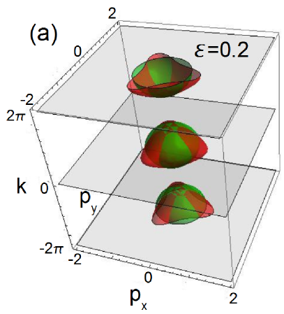
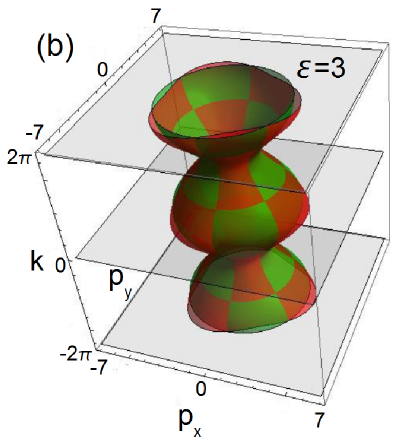
Figure 13: (Color online) Isoenergetic surfaces $\varepsilon(p_{x},p_{y},k)=\varepsilon=\rm const$ are shown for $\varepsilon=0.2$ and $\varepsilon=3$ in panels (a) and (b), respectively. The green cylindrically-symmetric surfaces correspond to Hamiltonian (18), and the red trigonally-warped surfaces to Hamiltonian (61).

Trigonal warping of the isoenergetic surfaces becomes progressively more pronounced at low energies $|\varepsilon|<0.1$. At much lower energies $\varepsilon\sim 0.01$, the isoenergetic surface spits into four separate branches with three new Dirac points surrounding the original Dirac point Brandt ; Gruneis . For such low energies, the isoenergetic surfaces qualitatively differ from the case of $\gamma_{3}=0$, and our results are not applicable. At the low energies, it is also necessary to take into account the other tunneling amplitudes, in particular $\gamma_{2}\sim 10$ meV, which connects the next-nearest layers Gruneis . In the presence of many tunneling amplitudes, the problem becomes very complicated. In addition, disorder may smear out the spectrum at low energies.

Thus, we restrict the applicability of our results to the relatively high energies $|\varepsilon|>0.1$, which is about 40 meV in the dimensional units. The energy spectrum in this range can be studied by tunneling or optical spectroscopy. Notice that the magnetic-field-dependent peak in $dI/dV$ was observed in Ref. Latyshev-2010 at the applied voltage of about 80 meV, although exact nature of this peak is still unclear.

References

- (1) K. S. Novoselov, A. K. Geim, S. V. Morozov, D. Jiang, Y. Zhang, S. V. Dubonos, I. V. Grigorieva, and A. A. Firsov, Science 306, 666 (2004).
- (2) K. S. Novoselov, A. K. Geim, S. V. Morozov, D. Jiang, M. I. Katsnelson, I. V. Grigorieva, S. V. Dubonos, and A. A. Firsov, Nature 438, 197 (2005).
- (3) Y. Zhang, Y.-W. Tan, H. L. Stormer, and P. Kim, Nature 438, 201 (2005).
- (4) M. L. Sadowski, G. Martinez, M. Potemski, C. Berger and W. A. de Heer , Phys. Rev. Lett. 97, 266405 (2006).
- (5) V. P. Gusynin and S. G. Sharapov, Phys. Rev. Lett. 95, 146801 (2005).
- (6) Z. Jiang, E. A. Henriksen, L. C. Tung, Y.-J. Wang, M. E. Schwartz, M. Y. Han, P. Kim, and H. L. Stormer, Phys. Rev. Lett. 98, 197403 (2007).
- (7) E. McCann and V. I. Fal’ko, Phys. Rev. Lett. 96, 086805 (2006).
- (8) M. Inoue, J. Phys. Soc. Jpn. 17, 808 (1962).
- (9) G. Dresselhaus, Phys. Rev. B 10, 3602 (1974).
- (10) N. B. Brandt, S. M. Chudinov, and Ya. G. Ponomarev, Semimetals: Graphite and Its Compounds (North-Holland, Amsterdam, 1988).
- (11) G. Li and E. Y. Andrei, Nat. Phys. 3, 653 (2007).
- (12) P. Plochocka, C. Faugeras, M. Orlita, M. L. Sadowski, G. Martinez, M. Potemski, M. O. Goerbig, J.-N. Fuchs, C. Berger and W. A. de Heer, Phys. Rev. Lett. 100, 087401 (2008).
- (13) M. Orlita, C. Faugeras, J. M. Schneider, G. Martinez, D. K. Maude, and M. Potemski, Phys. Rev. Lett. 102, 166401 (2009).
- (14) K.-C. Chuang, A. M. R. Baker, and R. J. Nicholas, Phys. Rev. B 80, 161410 (R) (2009).
- (15) A. F. Garcia-Flores, H. Terashita, E. Granado, and Y. Kopelevich, Phys. Rev. B 79, 113105 (2009).
- (16) M. Koshino and T. Ando, Phys. Rev. B 77, 115313 (2008).
- (17) F. Guinea, A. H. Castro Neto, and N. M. R. Peres, Phys. Rev. B 73, 245426 (2006).
- (18) Y. Kopelevich, P. Esquinazi, J. H. S. Torres, and S. Moehlecke, J. Low Temp. Phys. 119, 691 (2000); H. Kempa, H. C. Semmelhack, P. Esquinazi, and Y. Kopelevich, Solid State Comm. 125, 1 (2003).
- (19) Y. Iye, M. Baxendale, and V. Z. Mordkovich, J. Phys. Soc. Jpn. 63, 1643 (1994).
- (20) M. V. Kartsovnik, P. A. Kononovich, V. N. Laukhin, and I. F. Schegolev, JETP Lett. 48, 541 (1988).
- (21) K. Kajita, Y. Nishio, T. Takahashi, W. Sasaki, R. Kato, H. Kobayashi, A. Kobayashi, and Y. Iye, Solid State Comm. 70, 1189 (1989).
- (22) V. M. Yakovenko and B. K. Cooper, Physica E 34, 128 (2006).
- (23) M. S. Dresselhaus and G. Dresselhaus, Adv. Phys. 51, 1 (2002).
- (24) Yu. I. Latyshev, A. P. Orlov, A. Yu. Latyshev, and W. Escoffier, Proceedings of the XIV Symposium on Nanophysics and Nanoelectronics, Nizhni Novgorod (2010), in Russian.
- (25) V. M. Krasnov, A. Yurgens, D. Winkler, P. Delsing, and T. Claeson, Phys. Rev. Lett. 84, 5860 (2000).
- (26) Yu. I. Latyshev, P. Monceau, S. Brazovskii, A. P. Orlov, and T. Fournier, Phys. Rev. Lett. 95, 266402 (2005).
- (27) A. Grüneis, C. Attaccalite, L. Wirtz, H. Shiozawa, R. Saito, T. Pichler, and A. Rubio, Phys. Rev. B 78, 205425 (2008).
- (28) E. H. Hwang and S. Das Sarma, Phys. Rev. B 80, 075417 (2009).
- (29) V. M. Yakovenko, Europhys. Lett. 3, 1041 (1987); Sov. Phys. JETP 66, 355 (1987).
- (30) V. M. Yakovenko and H. -S. Goan, Phys. Rev. B 58, 8002 (1998).
- (31) A. G. Lebed, Phys. Rev. Lett. 95, 247003 (2005).
- (32) The Physics of Organic Superconductors and Conductors, edited by A. G. Lebed (Springer, Berlin, 2008).
- (33) J. M. B. Lopes dos Santos, N. M. R. Peres, and A. H. Castro Neto, Phys. Rev. Lett. 99, 256802 (2007).
- (34) Guohong Li, A. Luican, J. M. B. Lopes dos Santos, A. H. Castro Neto, A. Reina, J. Kong and E. Y. Andrei, Nat. Phys. 6, 109 (2010).
- (35) L. Onsager, Phil. Mag. 43, 1006 (1952).