The relationship between induced fluid structure and boundary slip in nanoscale polymer films
Abstract
The molecular mechanism of slip at the interface between polymer melts and weakly attractive smooth surfaces is investigated using molecular dynamics simulations. In agreement with our previous studies on slip flow of shear-thinning fluids, it is shown that the slip length passes through a local minimum at low shear rates and then increases rapidly at higher shear rates. We found that at sufficiently high shear rates, the slip flow over atomically flat crystalline surfaces is anisotropic. It is demonstrated numerically that the friction coefficient at the liquid-solid interface (the ratio of viscosity and slip length) undergoes a transition from a constant value to the power-law decay as a function of the slip velocity. The characteristic velocity of the transition correlates well with the diffusion velocity of fluid monomers in the first fluid layer near the solid wall at equilibrium. We also show that in the linear regime, the friction coefficient is well described by a function of a single variable, which is a product of the magnitude of surface-induced peak in the structure factor and the contact density of the adjacent fluid layer. The universal relationship between the friction coefficient and induced fluid structure holds for a number of material parameters of the interface: fluid density, chain length, wall-fluid interaction energy, wall density, lattice type and orientation, thermal or solid walls.
pacs:
68.08.-p, 83.80.Sg, 83.50.Rp, 47.61.-k, 83.10.RsI Introduction
The study of fluid transport through micro- and nanochannels is important for biotechnological applications and energy conversion processes Eijkel09 . The precise control and manipulation of fluids in systems with large surface-to-volume ratios, however, require fundamental understanding of flow boundary conditions. Fluid velocity profiles can be significantly modified in the presence of slip at a solid surface. The degree of slip is quantified by the slip length, which is defined as a distance between locations of the real interface and imaginary plane where the extrapolated tangential velocity component vanishes. It was shown by numerous experimental studies that the main factors affecting slippage at the liquid-solid interface include surface roughness Granick02 ; Archer03 ; Leger06 , surface wettability Churaev84 ; Charlaix01 ; SchmatkoPRL05 , fluid structure SchmatkoPRL05 ; BruceLaw09 ; Jacobs09 , and shear rate Granick01 ; Breuer03 ; Ulmanella08 . The slip length in the micron range is reported for complex flows near superhydrophobic surfaces Rothstein10 and flows of high molecular weight polymers JacobsRev , while the magnitude of the slip length in the range of a few tens of nanometers is typically measured for flows of water over smooth nonwetting surfaces Charlaix10 .
A number of molecular dynamics (MD) simulation studies have been carried out to investigate the influence of structural properties of the interface between monatomic fluids and flat crystalline walls on the degree of slip Fischer89 ; KB89 ; Thompson90 ; Barrat94 ; Nature97 ; Barrat99 ; Barrat99fd ; Attard04 ; Priezjev07 ; PriezjevJCP ; Li09 ; Asproulis10 . It was shown that the slip length is directly related to the intensity of structure induced in the first fluid layer by the periodic potential from the solid substrate Thompson90 . The slip is reduced with increasing wall-fluid interaction energy and due to the formation of commensurate structures between solid wall and adjacent fluid layer. The solid walls are usually modeled as an array of atoms arranged on sites of a periodic lattice. Two types of walls are considered, solid and thermal, where the wall atoms are either fixed at the lattice sites or allowed to oscillate in the harmonic potential. It was found that the slip length weakly depends on the value of the spring stiffness coefficient for sufficiently strong harmonic bonds PriezjevJCP ; Asproulis10 . In addition, the slope of the shear rate dependence of the slip length is not significantly affected by stiff springs PriezjevJCP , except at very high shear rates LichPRL08 .
At the interface between simple fluids and atomically smooth, weakly attractive surfaces, the slip length is constant at low shear rates and increases nonlinearly at higher shear rates, as originally discovered by Thompson and Troian Nature97 and later confirmed by several studies Fang05 ; Priezjev07 ; Niavarani10 ; Asproulis10 . For sufficiently strong wall-fluid interactions and incommensurate structures of the liquid and solid phases at the interface, the slip length varies almost linearly with shear rate Priezjev07 ; PriezjevJCP . It should be noted, however, that if the slip length at low shear rates is less than about a molecular diameter then the boundary conditions for dense monatomic fluids are rate-independent Thompson90 ; Nature97 ; PriezjevJCP . Also, it was shown that molecular-scale surface roughness reduces the magnitude of the slip length and the slope of its rate dependence Barrat94 ; Priezjev06 ; PriezjevJCP ; Sofos09 ; Niavarani10 .
It was recently demonstrated that the effective slip length for flows over anisotropic surfaces with two-component texture of different wettability is largest (smallest) for parallel (perpendicular) orientation of stripes with respect to the mean flow Vinograd09 . These conclusions hold when the stripe width is comparable to the molecular diameter Priezjev05 . For the transverse orientation of the flow relative to the stripes, the slip is reduced because of the molecular scale corrugation of the composed surface potential, while for the parallel orientation, the fluid molecules are transported along homogeneous stripes with either no-slip or partial slip conditions, and, therefore, the effective slip length is enhanced Priezjev05 . More recently, it was observed that the slip length also depends on the crystal lattice plane in contact with the fluid and on the lattice orientation with respect to the flow direction Tzeng07 . In the present study, we will show that at sufficiently high shear rates, the slip flow is anisotropic for atomically flat crystalline surfaces; and, in particular, the slip length is enhanced when the shear flow is oriented along the crystallographic axis of the wall lattice.
Recent studies of friction between adsorbed monolayers and smooth crystalline surfaces are relevant to the analysis of flow boundary conditions Robbins96 ; Tomassone97 . It was found that the slip time, which represents the transfer of momentum between the adsorbed monolayer and the substrate, is proportional to the phonon lifetime divided by the normalized peak value of the structure factor computed in the monolayer at the main reciprocal lattice vector Robbins96 . Also, the simulation results have shown that the slip time is independent of the sliding direction if the slip velocity of the monolayer is much smaller than the speed of sound Robbins96 . In the linear regime between friction force and sliding velocity and in the range of film coverages from submonolayer to bilayer, the slip times were computed directly from the decay of the film velocity and from the decay of the velocity correlation function at equilibrium Tomassone97 .
During the last two decades, several MD studies have examined slip boundary conditions at the interface between polymeric fluids and flat crystalline surfaces Thompson95 ; Manias96 ; dePablo96 ; StevensJCP97 ; Koike98 ; Tanner99 ; Priezjev04 ; Priezjev08 ; Servantie08 ; Priezjev09 ; Hendy09 . The velocity profiles with stick boundary conditions were observed when a highly viscous interfacial layer was formed because of the strong wall-fluid interaction energy Tanner99 ; Manias96 ; Servantie08 , high fluid density and pressure Thompson95 ; Manias96 ; Priezjev09 , or chemical structure of chain molecules Denniston10 . The variation of the slip length as a function of shear rate was reported for flat polymer-solid interfaces with weak wall-fluid interactions Tanner99 ; Priezjev04 ; Niavarani08 ; Priezjev08 ; LichPRL08 ; Priezjev09 ; Hendy09 . In our previous studies Niavarani08 ; Priezjev08 , it was shown that the rate dependence of the slip length acquires a local minimum at low shear rates followed by a rapid growth at higher shear rates. Furthermore, it was found that in a wide range of fluid densities, the friction coefficient at the liquid-solid interface undergoes a gradual transition from a constant value to the power-law decay as a function of the slip velocity Priezjev08 ; Priezjev09 . Remarkably, the data for the friction coefficient at different fluid densities and shear rates were found to collapse onto a master curve when plotted as a function of the product of the main peak in the structure factor and the contact density of the first fluid layer Priezjev08 ; Priezjev09 . Although promising results were obtained, the simulations were performed at a single wall density and only for one orientation of the fcc lattice with respect to the shear flow direction Priezjev08 ; Priezjev09 .
In this paper, molecular dynamics simulations were conducted for twenty systems that include monatomic and polymeric fluids confined by flat crystalline surfaces. In agreement with previous studies, we report the nonlinear rate dependence of the slip length for systems with weak wall-fluid interaction energies and relatively dense walls. The simulation results indicate that the friction coefficient (the ratio of fluid viscosity and slip length) in the linear-response regime is a function of a single variable that is a product of the height of the normalized main peak in the structure factor and the contact density of the first fluid layer near the solid wall. We will show that the onset of the nonlinear regime between the wall shear stress and slip velocity is determined by the diffusion of fluid monomers within the first layer.
The rest of the paper proceeds as follows. The details of molecular dynamics simulations and parameter values for twenty systems are described in the next section. The results for the rate-dependent slip length, friction coefficient, and fluid structure are presented in Section III. The conclusions are given in the last section.
II Molecular dynamics simulation model and parameter values
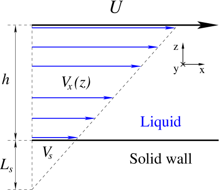
The geometry of the computational domain and the steady flow profile are shown schematically in Figure 1. The fluid undergoes planar shear flow between two atomically flat walls. The fluid phase consists of monomers. The interaction between any two fluid monomers is modeled via the truncated Lennard-Jones (LJ) potential
| (1) |
where and are the energy and length scales of the fluid phase and is a cutoff radius. The interaction between the wall atoms and fluid monomers is also modeled by the LJ potential with parameters (listed in Table 1) and . The wall atoms do not interact with each other via the LJ potential.
Three types of fluid were considered in the present study, i.e., monomeric (or simple) fluid and polymer melts with the number of monomers per chain and . In the case of polymers, the nearest-neighbor monomers in a chain interact through the finitely extensible nonlinear elastic (FENE) potential Bird87
| (2) |
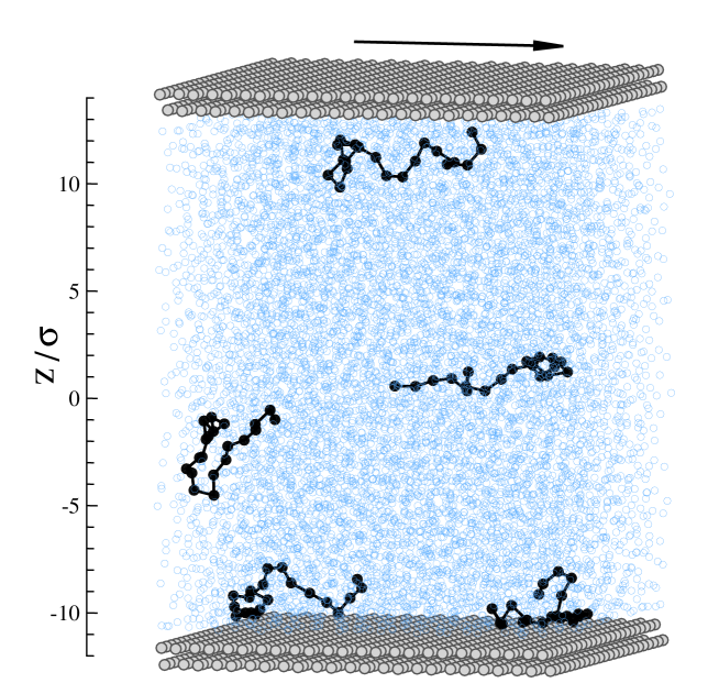
with the energy and length parameters and introduced by Kremer and Grest Kremer90 . Figure 2 shows a snapshot of an unentangled polymer melt with linear flexible chains confined between solid walls.
The heat exchange between the fluid phase and the external heat bath was regulated via a Langevin thermostat Grest86 , which was applied only to the direction of motion perpendicular to the plane of shear Thompson90 . The equations of motion for fluid monomers in all three directions are given as follows:
| (3) | |||||
| (4) | |||||
| (5) |
where the summation is performed over the fluid monomers and wall atoms within the cutoff radius , is the friction coefficient, and is a random force with zero mean and variance determined from the fluctuation-dissipation theorem. The thermostat temperature is , where is the Boltzmann constant. The equations of motion were integrated using the fifth-order gear-predictor algorithm Allen87 with a time step , where is the characteristic time of the LJ potential. The small time step was used in our previous studies Priezjev07 ; Priezjev08 ; Priezjev09 for similar MD setups in order to compute accurately the trajectories of fluid molecules and wall atoms near interfaces.
Each confining wall is composed of atoms arranged in two layers of the face-centered cubic (fcc) or body-centered cubic (bcc) lattice. The wall density, lattice type, its orientation with respect to the shear flow direction, and wall-fluid interaction energy are reported in Table 1. The wall atoms were either fixed at the lattice sites or were allowed to oscillate about their equilibrium lattice positions under the harmonic potential with the spring stiffness coefficient . In the latter case, the Langevin thermostat was applied to the , and components of the wall atom equations of motion. For example, the component of the equation of motion is given by
| (6) |
where , the friction coefficient is and the sum is taken over the neighboring fluid monomers within the cutoff radius . Periodic boundary conditions were imposed along the the and directions parallel to the confining walls.
Initially, the fluid was equilibrated at a constant normal pressure (shown in Table 1) for about . Then, the channel height was fixed and the system was additionally equilibrated for at a constant density ensemble. The steady flow was generated by moving the upper wall with a constant speed in the direction parallel to the immobile lower wall (see Fig. 1). The lowest speed of the upper wall is . Both fluid velocity and density profiles were computed within horizontal bins of thickness for a time period up to .
III Results
III.1 Fluid density and velocity profiles
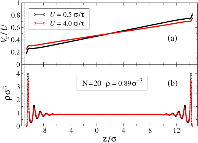
The averaged fluid density and velocity profiles are presented in Fig. 3 for the upper wall speeds and . The density profiles exhibit a typical layered structure which extends for about away from the solid walls. The amplitude of the first peak in the density profile determines the contact density . We emphasize that the thickness of the averaging bins is small enough so that the magnitude of the peaks does not depend on the bin thickness and bin location relative to the walls. On the other hand, the shape of the density profiles will remain unchanged if thinner bins are used; however, the averaging is computationally more expensive. As evident from Fig. 3 (b), the contact density is reduced at higher upper wall speeds.
Two representative velocity profiles normalized by the upper wall speed are shown in Fig. 3 (a). The slip velocity increases at higher upper wall speeds. The location of the liquid-solid interface (marked by the dashed vertical lines in Fig. 3) is defined at the distance away from the wall lattice planes to take into account the excluded volume due to wall atoms. The slip length was computed from the linear fit to the velocity profiles excluding regions of about from the solid walls. At all shear rates examined in the present study, the velocity profiles are linear across the channel and the slip length is larger than about .
III.2 Rate dependence of viscosity and slip length
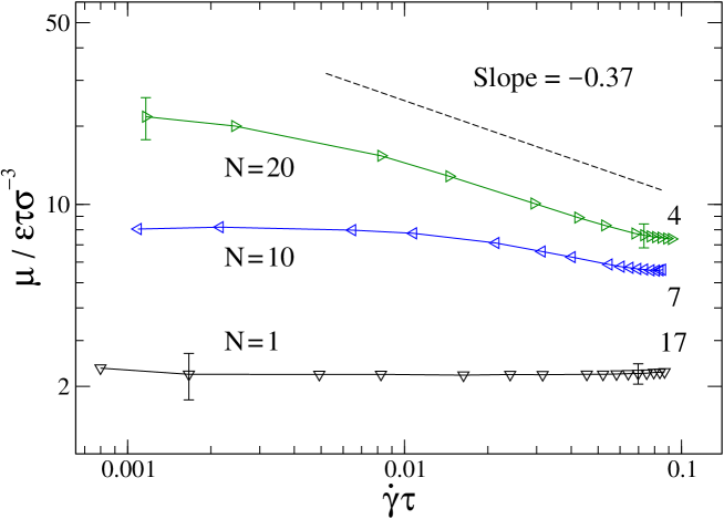
The fluid viscosity was estimated from the relation between shear rate and shear stress which was computed using the Kirkwood formula Kirkwood . The variation of viscosity as a function of shear rate is presented in Fig. 4 for selected systems listed in Table 1. In agreement with previous studies with a similar setup Nature97 ; Priezjev07 ; PriezjevJCP , the viscosity of monatomic fluids is independent of shear rate and equals when the fluid density is . As expected, the shear viscosity of polymer melts with chains and is higher than the viscosity of simple monatomic fluids. For similar flow conditions, the transition from a Newtonian to a shear-thinning flow regime occurs at lower shear rates for polymers with longer chains because of their slower intrinsic relaxation. The slope of the shear-thinning region shown in Fig. 4 is consistent with the results reported in earlier studies for polymer melts at different densities Priezjev08 ; Priezjev09 . The errors arising from averaging over thermal fluctuations are greater at lower shear rates.
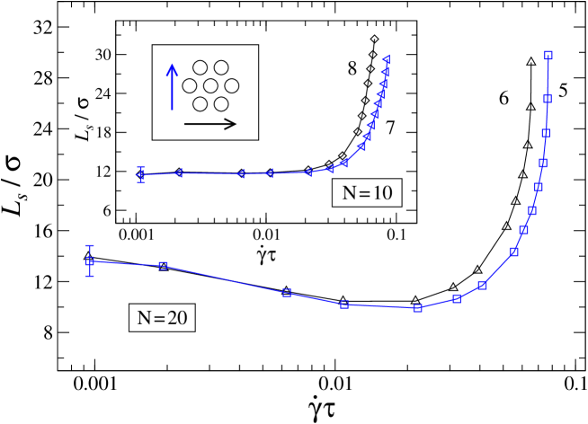
The nonlinear rate dependence of the slip length is shown in Fig. 5 for polymer melts with chains and . The shear flow direction is oriented along the crystallographic axis of the plane of the fcc wall lattice for systems and (see Table 1). In contrast, the fcc lattice plane is rotated by with respect to the flow direction for systems and as indicated by open circles and blue vertical arrow in the inset of Fig. 5. At low shear rates , the slip length is independent of the wall lattice orientation relative to the shear flow direction; while at higher shear rates, the slip length is greater when the shear flow is parallel to the crystallographic axis of the triangular lattice. The same trend for the slip length is observed for monatomic fluids (not shown). These results demonstrate that at sufficiently high shear rates the slip flow is anisotropic even for atomically flat crystalline surfaces.
The appearance of the local minimum in the rate dependence of the slip length reported in Fig. 5 for polymer melts with chains was explained in the previous MD study Priezjev08 . The initial decay of the slip length at low shear rates is associated with a slight decrease in the melt viscosity while the friction coefficient at the liquid-solid interface () remains constant (see also next section). With increasing shear rate, the friction coefficient decreases faster than the shear viscosity, and, therefore, the slip length grows rapidly Priezjev08 ; Niavarani08 . Since the transition to the shear-thinning regime occurs at higher shear rates for polymer melts with shorter chains , the slip length remains nearly constant at low shear rates and then increases rapidly at higher rates (see inset in Fig. 5). These results agree well with the previous simulation results for slip flow of polymers with chain lengths and lower fluid density Priezjev04 .
III.3 Friction coefficient versus slip velocity
The relation between the slip length and shear rate can be expressed in terms of the friction coefficient at the liquid-solid interface and slip velocity. In steady-state shear flow, the shear stress in the bulk of the film () is equal to the wall shear stress (). In addition, if the velocity profile is linear across the channel, then by definition and the friction coefficient is given by . In the previous MD study, the slip flow of polymer melts with chains was studied in the range of fluid densities , and velocity profiles were found to be linear at all shear rated examined Priezjev08 . Furthermore, the friction coefficient () as a function of the slip velocity could be well fitted by the following equation:
| (7) |
where is the friction coefficient at small slip velocities when and is the characteristic slip velocity that determines the onset of the nonlinear regime Priezjev08 . In the later study, the simulations were performed at higher melt densities and the velocity profiles at low shear rates were curved near interfaces, and, as a result, the definition could not be applied Priezjev09 . Therefore, the friction coefficient was computed directly from the ratio of the wall shear stress and slip velocity of the first fluid layer. For polymer melt densities and , the data were also well described by Eq. (7), while at higher melt densities () only the nonlinear regime was observed Priezjev09 .
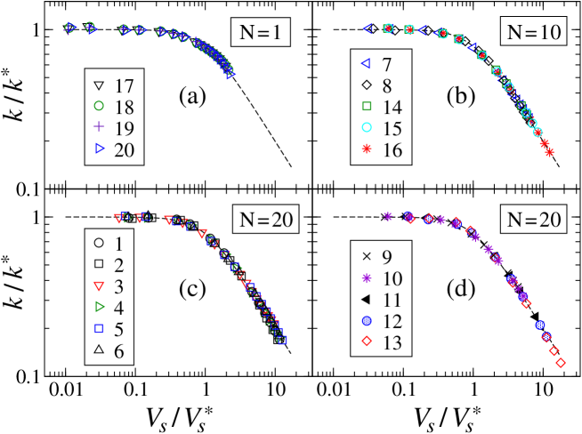
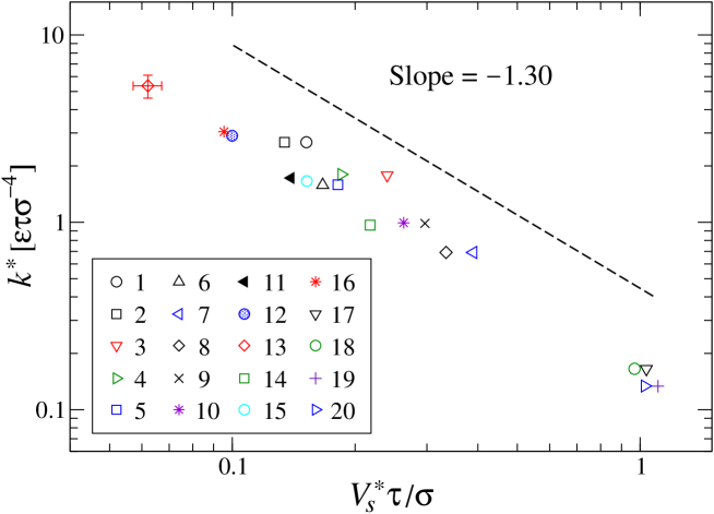
In the present study, we extend the analysis of the friction coefficient at the interface between crystalline walls and polymeric fluids described by the parameters listed in Table 1. Figure 6 shows the friction coefficient as a function of the slip velocity normalized by the parameters and respectively. The data for all systems in Table 1 are well fitted by Eq. (7) over about three orders of magnitude. We also noticed the inverse correlation between the friction coefficient and the characteristic slip velocity (shown in Fig. 7). Note that for every two systems with different orientation of the fcc wall lattice, the values of are nearly the same, but the slip velocity is slightly smaller when the shear flow direction is parallel to the crystallographic axis. This is consistent with the dynamic response of the slip length reported in Fig. 5 for two different orientations of the fcc lattice.
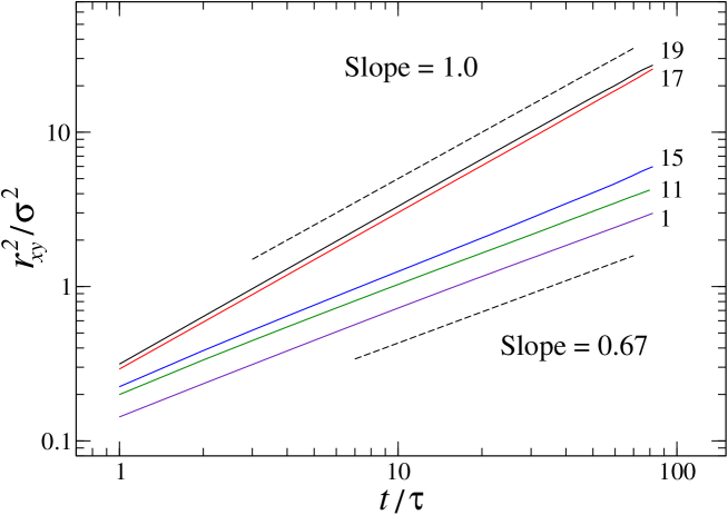
We next argue that the onset of the nonlinear regime in Eq. (7) is determined by the intrinsic relaxation time of the fluid monomers in the first layer near the solid wall. In Figure 8 we plot the mean square displacement of fluid monomers within the first layer for selected systems in Table 1 at equilibrium (i.e., when both walls are at rest). The displacement as a function of time was computed along the trajectory of a fluid monomer only if it remained in the first fluid layer during the time interval between successive measurements of the monomer position. For monatomic fluids, there is a linear dependence between the mean square displacement and time, and, consequently, the diffusion coefficient is well defined. This behavior agrees well with the exponential relaxation of the density-density autocorrelation function evaluated at the wavevector of about in the first layer of monatomic fluids confined by atomistic walls Barrat99fd ; Priezjev04 . In contrast, fluid monomers that belong to a polymer chain diffuse slower than monomers in simple fluids since their dynamics is bounded by diffusion of the center of mass of the polymer chain. The slope of the subdiffusive regime is shown in Fig. 8 by the straight dashed line.
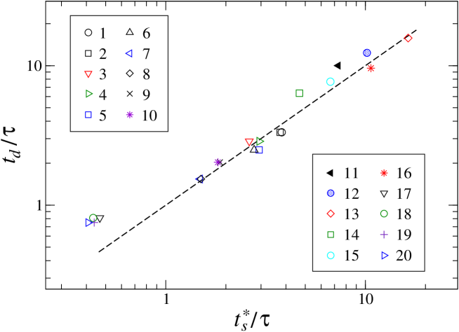
Finally, the comparison of the characteristic slip time of the first fluid layer and the diffusion time of fluid monomers between nearest minima of the surface potential is presented in Fig. 9. The diffusion time was estimated from the mean square displacement of fluid monomers in the first layer at the distance between nearest minima of the periodic surface potential. The same distance divided by the slip velocity defines the characteristic slip time of the first fluid layer. In the case when the shear flow direction is parallel to the fcc lattice orientation (e.g., see inset in Fig. 5), the slipping distance of the first layer was computed by projecting the vector, which connects nearest minima of the surface potential, onto the direction of flow. Figure 9 shows a strong correlation between the characteristic slip time of the adjacent fluid layer and the diffusion time of fluid monomers in that layer at equilibrium. These results indicate that the linear-response regime in Eq. (7) holds when the slip velocity is smaller than the diffusion velocity of fluid monomers in contact with flat crystalline walls.
III.4 Friction coefficient and induced fluid structure
The fluid structure near flat solid walls is characterized by density layering perpendicular to the surface and ordering of fluid monomers within the layers Kaplan06 . Examples of oscillatory density profiles in a polymer melt near confining walls were presented in Fig. 3. It is intuitively expected that enhanced fluid density layering normal to the surface (obtained, for example, by increasing fluid pressure or wall-fluid interaction energy) would correspond to a larger friction coefficient at the liquid-solid interface. However, this correlation does not always hold; for example, the amplitude of fluid density oscillations near flat structureless walls might be large, but the friction coefficient is zero. As emphasized in the original paper by Thompson and Robbins Thompson90 , the surface-induced fluid ordering within the first layer of monomers correlates well with the degree of slip at the liquid-solid interface. The measure of the induced order in the adjacent fluid layer is the static structure factor, which is defined as follows:
| (8) |
where is a two-dimensional wavevector, is the position vector of the -th monomer, and is the number of monomers within the layer Thompson90 . The probability of finding fluid monomers is greater near the minima of the periodic surface potential, and, therefore, the structure factor typically contains a set of sharp peaks at the reciprocal lattice vectors. It is well established that the magnitude of the largest peak at the first reciprocal lattice vector is one of the main factors that determine the value of the slip length at the interface between flat crystalline surfaces and monatomic fluids Thompson90 ; Barrat99fd ; Priezjev07 ; PriezjevJCP or polymer melts Thompson95 ; Priezjev04 ; Priezjev08 ; Priezjev09 .
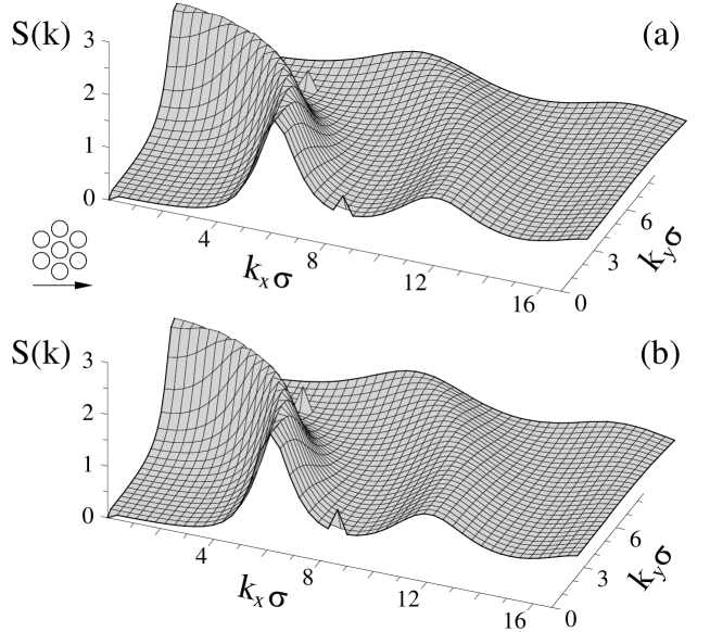
Next, we discuss the influence of the wall-fluid interaction energy, wall lattice type and orientation, and slip velocity on the structure factor computed in the first fluid layer. The effect of the wall-fluid interaction energy is illustrated in Fig. 10 for monatomic fluids in contact with the plane of the fcc wall lattice. The height of the surface-induced peaks in the structure factor is slightly larger at higher surface energy. The magnitude of the peak in the shear flow direction is for and for . Notice that the height of the circular ridge characteristic of short range ordering of fluid monomers is larger than the amplitude of the induced peaks at the reciprocal lattice vectors. A similar trend in the height of the peaks in the structure factor was observed previously for monatomic fluids confined by the fcc walls with higher density Priezjev07 .
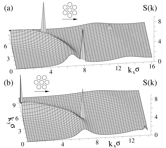
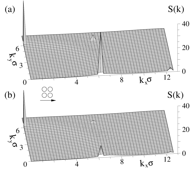
Figure 11 shows the structure factor computed in the first fluid layer for polymer melts with chains in contact with the plane of the fcc wall lattice. Due to the hexagonal symmetry of the lattice, the structure factor exhibits six peaks at the shortest reciprocal lattice vectors. Note that only two main peaks are present in the first quadrant. The magnitude of the peaks is the same at small slip velocities. The lattice orientation with respect to the shear flow direction determines the location of the main peaks. Finally, the effect of slip velocity on the magnitude of the substrate-induced peaks in the structure factor is presented in Fig. 12 for the polymer melt near the plane of the bcc wall lattice. With increasing slip velocity, the height of the induced peak along the shear flow direction decreases significantly, whereas the magnitude of the peak in the perpendicular direction is less affected by slip. In contrast to monatomic fluids, the amplitude of the peak due to short range order of monomers that belong to polymer chains is much smaller than the magnitude of the induced peaks at the shortest reciprocal lattice vectors (see Fig. 12).
The correlation between surface-induced structure in the first fluid layer and the friction coefficient was investigated previously for polymer melts with chains confined by atomically flat walls Priezjev08 ; Priezjev09 . The simulations were performed at fluid densities and the wall density . It was found that the data for the friction coefficient at different shear rates and fluid densities collapsed onto a master curve when plotted as a function of a variable , where is the first reciprocal lattice vector in the shear flow direction Priezjev08 ; Priezjev09 . The collapse of the data holds at relatively small values of the friction coefficient and for slip lengths larger than approximately . Although these results are promising, the simulations were limited to a single wall density and the orientation of the plane of the fcc wall lattice.
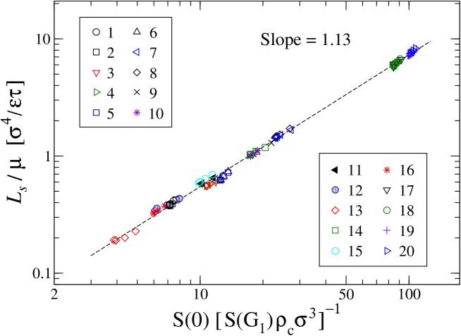
In the present study, a number of parameters that affect slippage at the liquid-solid interface have been examined, i.e., fluid and wall densities, polymer chain length, wall lattice type and orientation, wall-fluid interaction energy, thermal and solid walls (see Table 1). We first consider the linear-response regime where the friction coefficient weakly depends on the slip velocity ( in Fig. 6). Figure 13 shows the ratio (an inverse friction coefficient) as a function of the variable computed in the first fluid layer for twenty systems listed in Table 1. In the case when the shear flow direction is parallel to the orientation of the fcc lattice [e.g., see Fig. 11 (b)], the structure factor was computed at the shortest reciprocal lattice vector aligned at an angle of with respect to the axis. Since the magnitude of the surface-induced peaks in the structure factor scales with the number of monomers in the first fluid layer, the height of the main peak was normalized by the average number of monomers in the layer . The data in Fig. 6 are well described by a power-law fit with the slope . These results suggest that at the interface between simple or polymeric fluids and flat crystalline surfaces, the ratio of the slip length and viscosity at low shear rates [ or the value of parameter in Eq. (7) ] can be estimated from equilibrium measurements of the structure factor and the contact density of the first fluid layer.
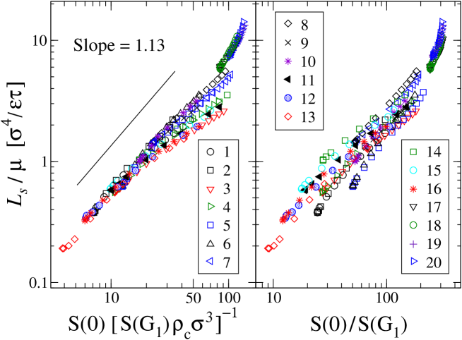
In Figure 14 we report the dependence of the friction coefficient () on the structure factor and contact density of the first fluid layer at all shear rates examined in this study (the same data as in Fig. 6). Note that at higher shear rates the derivative of with respect to for several systems listed in Table 1 deviates significantly from the slope shown for reference in Fig. 14 (a). In addition, for any two systems with the same and , the ratio as a function of depends on the orientation of the fcc wall lattice with respect to the shear flow direction. Although the data in Fig. 14 (b) are somewhat scattered, the results show the same trend, namely, the friction coefficient decreases when the magnitude of the normalized peak in the structure factor is reduced. The collapse of the data for versus was reported in Ref. Thompson90 for monatomic fluids and crystalline walls when and the boundary conditions are rate independent. In the present study, the slip lengths are greater than about except for the systems and where at low shear rates. We finally comment that our results were not analyzed with respect to the relation (between the friction coefficient and induced fluid structure and in-plane diffusion coefficient) derived in Ref. Barrat99fd for simple fluids, because the slope of the mean square displacement versus time for polymer systems (shown in Fig. 8) is less than one and thus the diffusion coefficient is not well defined.
IV Conclusions
In this paper, we investigated the dynamic behavior of the slip length at interfaces between polymeric or monatomic fluids and flat crystalline surfaces using molecular dynamics simulations. The polymer melt was modeled as a collection of bead-spring linear flexible chains below the entanglement length. We considered shear flow conditions at relatively low fluid densities (pressures) and weak wall-fluid interaction energies so that fluid velocity profiles are linear across the channel at all shear rates examined. It was found that the slip length does not depend on the wall lattice orientation with respect to the flow direction only at low shear rates, whereas the slip is enhanced at high shear rates when the flow direction is parallel to the crystallographic axis of the substrate.
In the steady shear flow of either monatomic fluids or polymer melts, the friction coefficient at the liquid-solid interface (computed from the ratio of fluid viscosity and slip length) undergoes a transition from a constant value to the power-law decay as a function of the slip velocity. The characteristic velocity of the transition is determined by the diffusion of fluid monomers over the distance between nearest minima of the substrate potential. It is demonstrated that the friction coefficient at small slip velocities is a function of the magnitude of the surface-induced peak in the structure factor and the contact density of the first fluid layer. These conclusions hold for different wall and fluid densities, chain lengths, surface energies, lattice types and orientations, thermal or solid walls.
Acknowledgments
Financial support from the National Science Foundation and the Petroleum Research Fund of the American Chemical Society is gratefully acknowledged. Computational work in support of this research was performed at Michigan State University’s High Performance Computing Facility.
References
- (1) W. Sparreboom, A. van den Berg and J. C. T. Eijkel, Nature Nanotechnology 4, 713 (2009).
- (2) Y. Zhu and S. Granick, Phys. Rev. Lett. 88, 106102 (2002).
- (3) J. Sanchez-Reyes and L. A. Archer, Langmuir 19, 3304 (2003).
- (4) T. Schmatko, H. Hervet, and L. Leger, Langmuir 22, 6843 (2006).
- (5) N. V. Churaev, V. D. Sobolev, and A. N. Somov, J. Colloid Interface Sci. 97, 574 (1984).
- (6) J. Baudry, E. Charlaix, A. Tonck, and D. Mazuyer, Langmuir 17, 5232 (2001).
- (7) T. Schmatko, H. Hervet, and L. Leger, Phys. Rev. Lett. 94, 244501 (2005).
- (8) S. P. McBride and B. M. Law, Phys. Rev. E 80, 060601(R) (2009).
- (9) O. Baumchen, R. Fetzer, and K. Jacobs, Phys. Rev. Lett. 103, 247801 (2009).
- (10) Y. Zhu and S. Granick, Phys. Rev. Lett. 87, 096105 (2001).
- (11) C. H. Choi, K. J. A. Westin, and K. S. Breuer, Phys. Fluids 15, 2897 (2003).
- (12) U. Ulmanella and C.-M. Ho, Phys. Fluids 20, 101512 (2008).
- (13) J. P. Rothstein, Annu. Rev. Fluid Mech. 42, 89 (2010).
- (14) O. Baumchen and K. Jacobs, J. Phys. Condens. Matter 22, 033102 (2010).
- (15) L. Bocquet and E. Charlaix, Chem. Soc. Rev. 39, 1073 (2010).
- (16) U. Heinbuch and J. Fischer, Phys. Rev. A 40, 1144 (1989).
- (17) J. Koplik, J. R. Banavar, and J. F. Willemsen, Phys. Fluids A 1, 781 (1989).
- (18) P. A. Thompson and M. O. Robbins, Phys. Rev. A 41, 6830 (1990).
- (19) L. Bocquet and J.-L. Barrat, Phys. Rev. E 49, 3079 (1994).
- (20) J.-L. Barrat and L. Bocquet, Phys. Rev. Lett. 82, 4671 (1999).
- (21) J.-L. Barrat and L. Bocquet, Faraday Discuss. 112, 119 (1999).
- (22) T. M. Galea and P. Attard, Langmuir 20, 3477 (2004).
- (23) N. V. Priezjev, Phys. Rev. E 75, 051605 (2007).
- (24) N. V. Priezjev, J. Chem. Phys. 127, 144708 (2007).
- (25) P. A. Thompson and S. M. Troian, Nature (London) 389, 360 (1997).
- (26) C. Liu and Z. Li, Phys. Rev. E 80, 036302 (2009).
- (27) N. Asproulis and D. Drikakis, Phys. Rev. E 81, 061503 (2010).
- (28) A. Martini, H. Y. Hsu, N. A. Patankar, and S. Lichter, Phys. Rev. Lett. 100, 206001 (2008).
- (29) S. C. Yang and L. B. Fang, Molecular Simulation 31, 971 (2005).
- (30) A. Niavarani and N. V. Priezjev, Phys. Rev. E 81, 011606 (2010).
- (31) N. V. Priezjev and S. M. Troian, J. Fluid Mech. 554, 25 (2006).
- (32) F. D. Sofos, T. E. Karakasidis, and A. Liakopoulos, Phys. Rev. E 79, 026305 (2009).
- (33) F. Feuillebois, M. Z. Bazant, and O. I. Vinogradova, Phys. Rev. Lett. 102, 026001 (2009).
- (34) N. V. Priezjev, A. A. Darhuber, and S. M. Troian, Phys. Rev. E 71, 041608 (2005).
- (35) C. Y. Soong, T. H. Yen, P. Y. Tzeng, Phys. Rev. E 76, 036303 (2007).
- (36) P. A. Thompson, M. O. Robbins, and G. S. Grest, Israel Journal of Chemistry 35, 93 (1995).
- (37) E. Manias, G. Hadziioannou, and G. ten Brinke, Langmuir 12, 4587 (1996).
- (38) R. Khare, J. J. de Pablo, and A. Yethiraj, Macromolecules 29, 7910 (1996).
- (39) M. J. Stevens, M. Mondello, G. S. Grest, S. T. Cui, H. D. Cochran, and P. T. Cummings, J. Chem. Phys. 106, 7303 (1997).
- (40) A. Koike and M. Yoneya, J. Phys. Chem. B 102, 3669 (1998).
- (41) A. Jabbarzadeh, J. D. Atkinson, and R. I. Tanner, J. Chem. Phys. 110, 2612 (1999).
- (42) N. V. Priezjev and S. M. Troian, Phys. Rev. Lett. 92, 018302 (2004).
- (43) A. Niavarani and N. V. Priezjev, Phys. Rev. E 77, 041606 (2008).
- (44) J. Servantie and M. Muller, Phys. Rev. Lett. 101, 026101 (2008).
- (45) N. V. Priezjev, Phys. Rev. E 80, 031608 (2009).
- (46) S. Dhondi, G. G. Pereira, and S. C. Hendy, Phys. Rev. E 80, 036309 (2009).
- (47) L.-T. Kong, C. Denniston, and M. H. Muser, Modelling Simul. Mater. Sci. Eng. 18, 034004 (2010).
- (48) A. Niavarani and N. V. Priezjev, J. Chem. Phys. 129, 144902 (2008).
- (49) E. D. Smith, M. O. Robbins, and M. Cieplak, Phys. Rev. B 54, 8252 (1996).
- (50) M. S. Tomassone, J. B. Sokoloff, A. Widom, J. Krim, Phys. Rev. Lett. 79, 4798 (1997).
- (51) R. B. Bird, C. F. Curtiss, R. C. Armstrong, and O. Hassager, Dynamics of Polymeric Liquids 2nd ed. (Wiley, New York, 1987).
- (52) K. Kremer and G. S. Grest, J. Chem. Phys. 92, 5057 (1990).
- (53) G. S. Grest and K. Kremer, Phys. Rev. A 33, 3628 (1986).
- (54) M. P. Allen and D. J. Tildesley, Computer Simulation of Liquids (Clarendon, Oxford, 1987).
- (55) J. H. Irving and J. G. Kirkwood, J. Chem. Phys. 18, 817 (1950).
- (56) W. D. Kaplan and Y. Kauffmann, Annu. Rev. Mater. Res. 36, 1 (2006).