Competition between excitonic gap generation and disorder scattering in graphene

Abstract

We study the disorder effect on the excitonic gap generation caused by strong Coulomb interaction in graphene. By solving the self-consistently coupled equations of dynamical fermion gap $m$ and disorder scattering rate $\Gamma$, we found a critical line on the plane of interaction strength $\lambda$ and disorder strength $g$. The phase diagram is divided into two regions: in the region with large $\lambda$ and small $g$, $m\neq 0$ and $\Gamma=0$; in the other region, $m=0$ and $\Gamma\neq 0$ for nonzero $g$. In particular, there is no coexistence of finite fermion gap and finite scattering rate. These results imply a strong competition between excitonic gap generation and disorder scattering. This conclusion does not change when an additional contact four-fermion interaction is included. For sufficiently large $\lambda$, the growing disorder may drive a quantum phase transition from an excitonic insulator to a metal.

I Introduction

The low-energy elementary excitations in undoped graphene are massless Dirac fermions, which are believed to be responsible for the unusual physical properties of this material CastroNeto ; DasSarma ; Peres ; Mucciolo ; Ziegler ; Kotov . For clean undoped graphene, the density of states (DOS) of fermions $N(\omega)$ vanishes linearly near the Dirac point, so the Coulomb interaction between Dirac fermions is essentially unscreened CastroNeto ; Kotov ; Gonzalez94 . When the Coulomb interaction is sufficiently strong, $\lambda>\lambda_{c}$, it is able to open a finite gap for the Dirac fermions by forming stable excitonic pairs. Once this happens, the graphene then has an insulating ground state Kotov ; Khveshchenko00 ; Khveshchenko04 ; Gusynin ; Herbut ; Hands ; Drut09_1 ; Drut09_2 ; Liu ; Gamayun . This exotic insulator is induced by the strong electron-electron interaction and can be classified as a Mott insulator.

Although the excitonic insulating transition is a well-studied problem in graphene, so far little work has been devoted to the disorder effect on this nonperturbative phenomenon. In any realistic graphene, there are always some kinds of disorders, which affect significantly the low-energy transport properties of Dirac fermions. In practice, the scattering of Dirac fermions by disorder can result in important consequences Liu . On the one hand, the disorder scattering induces a finite density of states, $N(0)$, at the Fermi level. The finite $N(0)$ leads to static screening of the Coulomb interaction. Because the long-range nature of Coulomb interaction plays an essential role in producing excitonic pairing Liu , the fermion gap decreases with the growing disorder strength $g$ and might finally close when $g$ is greater than some critical value $g_{c}$. On the other hand, once the Dirac fermions acquire a finite gap due to excitonic pairing, the scattering rate and low-energy DOS will be quite different from those of gapless Dirac fermions. Therefore, fermion gap generation and disorder scattering are not independent. On the contrary, they have dramatic effects on each other and thus should be treated within a unified formalism. Technically, the fermion gap generation can be studied by the Dyson-Schwinger gap equation approach while the disorder scattering rate can be calculated by means of self-consistent Born approximation (SCBA). In order to examine the disorder effect on excitonic pairing, these two approaches should be combined properly.

In this paper, we examine the disorder effect on the excitonic fermion gap generation caused by Coulomb interaction in graphene. By solving the self-consistent equations for dynamical fermion gap $m$ and disorder scattering rate $\Gamma$, we found a critical line on the plane of interaction strength $\lambda$ and disorder strength $g$. This line separates two regions. In the region with large $\lambda$ and small $g$, $m\neq 0$ and $\Gamma=0$, so the ground state is an excitonic insulator with zero dc electric conductivity. In the other region, $m=0$ and $\Gamma\neq 0$ for nonzero $g$, so the Dirac fermions remain gapless and acquire a finite scattering rate. In this region, the dc electric conductivity is $\sigma=4e^{2}/\pi h$ to the leading order of Kubo formula, which is exactly quantized and independent of disorder. Apparently, the excitonic fermion gap generation due to Coulomb interaction competes strongly with the fermion damping effect caused by disorder scattering. As a consequence, the excitonic fermion gap and disorder scattering rate can not be finite simultaneously in graphene. If we fix the interaction parameter $\lambda$ at a sufficiently large value, then the graphene may undergo a first-order phase transition from an excitonic insulator to a metal at certain critical value $g_{c}$. These results indicate that the excitonic insulating phase transition can take place only in sufficiently clean graphene.

In addition to Coulomb interaction, there might be contact four-fermion interaction in realistic graphene. Such interaction is also able to generate a finite dynamical fermion gap when its strength is sufficiently large. In this paper, we also include the four-fermion interaction term in our self-consistent analysis and find that it does not change the conclusion. In particular, the excitonic fermion gap generation can not coexist with disorder scattering even when additional four-fermion interaction is taken into account.

The paper is organized as follows. In Sec.2, we study the self-consistent equations of excitonic fermion gap and disorder scattering rate when there is only Coulomb interaction. A strong competition between excitonic fermion gap generation and disorder scattering is found and a phase diagram on the $(\lambda,g)$ plane is presented. In Sec.3, we study the self-consistent equations in the presence of an additional contact four-fermion interaction. We show that such interaction does not change our phase diagram. In Sec.4, we discuss the physical implications of our result.

II Self-consistent analysis of excitonic transition and disorder scattering

The Hamiltonian of massless Dirac fermion with Coulomb interaction in graphene is given by

$$H = v_{F}\sum_{\sigma=1}^{N}\int_{\mathbf{r}}\bar{\psi}_{\sigma}(\mathbf{r})i\mathbf{\gamma}\cdot\mathbf{\nabla}\psi_{\sigma}(\mathbf{r})$$ (1)

$$+\frac{v_{F}}{4\pi}\sum_{\sigma,\sigma^{\prime}}^{N}\int_{\mathbf{r},\mathbf{r}^{\prime}}\bar{\psi}_{\sigma}(\mathbf{r})\gamma_{0}\psi_{\sigma}(\mathbf{r})\frac{\lambda}{|\mathbf{r}-\mathbf{r}^{\prime}|}\bar{\psi}_{\sigma^{\prime}}(\mathbf{r}^{\prime})\gamma_{0}\psi_{\sigma^{\prime}}(\mathbf{r}^{\prime}),$$

where the effective interaction strength is defined as $\lambda=2\pi e^{2}/v_{F}\epsilon$ with fermion velocity $v_{F}$ and dielectric constant $\epsilon$. As usual, we adopt the four-component spinor field $\psi$ to describe Dirac fermion and define the conjugate spinor field as $\bar{\psi}=\psi^{\dagger}\gamma_{0}$. The $4\times 4$ $\gamma$-matrices satisfy the Clifford algebra Khveshchenko00 ; *Khveshchenko04; Gusynin . The fermion flavor is taken to be $N$ and we will perform $1/N$ expansion since Coulomb interaction strength may be too large to be an expansion parameter. The disorder potential $U(\textbf{r})$ couples to fermion as

$$H_{\mathrm{dis}}=\sum_{\sigma=1}^{N}v_{F}\int_{\mathbf{r}}U(\textbf{r})\bar{\psi}_{\sigma}(\mathbf{r})\gamma_{0}\psi_{\sigma}(\mathbf{r}),$$ (2)

where $\langle U(\textbf{r})\rangle=0$ and $\langle U(\textbf{r})U(\textbf{r}^{\prime})\rangle=g\delta(\textbf{r}-\textbf{r}^{\prime})$. Here, $U(\textbf{r})$ plays the role of a random chemical potential and $g$ is the disorder strength parameter. For notational convenience, in the following discussion we will assume that $v_{F}=1$ and restore $v_{F}$ whenever necessary. The total Hamiltonian preserves a continuous chiral symmetry $\psi\rightarrow e^{i\theta\gamma_{5}}\psi$, where $\gamma_{5}$ anticommutes with $\gamma_{\mu}$, which will be dynamically broken once a nonzero fermion gap is generated.

The free propagator of Dirac fermion is

$$G_{0}^{-1}(i\omega_{n},\mathbf{k})=i\omega_{n}\gamma_{0}-\mathbf{\gamma}\cdot\mathbf{k},$$ (3)

where $\omega_{n}=(2n+1)\pi/\beta$ with $\beta=1/T$ and $n$ being integers. The Coulomb interaction and disorder scattering modify it to the form

$$G^{-1}(i\omega_{n},\mathbf{k})=(i\omega_{n}+i\mathrm{sgn}(\omega_{n})\Gamma)\gamma_{0}-\mathbf{\gamma}\cdot\mathbf{k}-m,$$ (4)

where $\Gamma$ is the scattering rate due to interaction. The fermion gap $m$ is generated by the excitonic pairing caused by Coulomb interaction and can be obtained from the following Dyson-Schwinger gap equation

$$G^{-1}(p) = G_{0}^{-1}(p)+\int\frac{d^{3}k}{(2\pi)^{3}}\gamma_{0}G(k)\gamma_{0}V(p-k),$$ (5)

to the leading order of $1/N$ expansion. The unscreened Coulomb interaction is $V_{0}(q)=\frac{\lambda}{|\mathbf{q}|}$. After including the dynamical screening effect from collective particle-hole excitations, the effective interaction function has the form

$$V(q)=\frac{1}{V_{0}^{-1}(q)+\Pi(q)}.$$ (6)

The polarization function is defined as

$$\Pi(q)=-N\int\frac{d^{3}k}{(2\pi)^{3}}\mathrm{Tr}\left[\gamma_{0}G(k)\gamma_{0}G(k+q)\right].$$ (7)

It has the simple form

$$\Pi(q)=\frac{N}{8}\frac{\mathbf{q}^{2}}{\sqrt{q_{0}^{2}+|\mathbf{q}|^{2}}},$$ (8)

to the leading order of $1/N$ expansion. It vanishes linearly as $\mathbf{q}\rightarrow 0$ in the static limit $q_{0}=0$, so the Coulomb interaction remains long-ranged. For physical flavor $N=2$, a sufficiently strong Coulomb interaction can trigger excitonic pairing instability, which generates a dynamical gap for Dirac fermions Kotov ; Khveshchenko00 ; *Khveshchenko04; Gusynin ; Herbut ; Hands ; Drut09_1 ; *Drut09_2; Liu ; Gamayun .

When disorder scattering is included, a finite fermion damping rate $\Gamma$ may be generated, which leads to two consequences. First, it changes the energy spectrum of fermions. Second, it yields a finite density of states at Fermi energy, which then screens the long-range Coulomb interaction. Both these effects are important and have to be incorporated into the gap equation. Because the sign of $\Gamma$ is determined by frequency $\omega_{n}$, the gap equation becomes much more complicated than that without $\Gamma$. To make our theoretical analysis tractable, here we adopt the frequently used instantaneous approximation Khveshchenko00 ; *Khveshchenko04; Gusynin . Taking trace on both sides of Eq.(5), we get

$$m(i\varepsilon_{n},\mathbf{p}) = \frac{1}{\beta}\sum_{\omega_{n}}\int\frac{d^{2}\mathbf{k}}{(2\pi)^{2}}\frac{m(i\omega_{n},\mathbf{k})}{(i\omega_{n}+i\Gamma\mathrm{sgn}(\omega_{n}))^{2}+|\mathbf{k}|^{2}+m^{2}(i\omega_{n},\mathbf{k})}$$ (9)

$$\times V(i\varepsilon_{n}-i\omega_{n},\mathbf{p}-\mathbf{k},\Gamma).$$

It is possible to sum over $\omega_{n}$ only when the frequency-dependence of fermion mass function is neglected, which is the so-called instantaneous approximation Khveshchenko00 ; *Khveshchenko04; Gusynin ; Liu . In this approximation, this equation becomes

$$m(\mathbf{p}) = \frac{1}{\beta}\sum_{\omega_{n}}\int\frac{d^{2}\mathbf{k}}{(2\pi)^{2}}\frac{m(\mathbf{k})}{(i\omega_{n}+i\Gamma\mathrm{sgn}(\omega_{n}))^{2}+|\mathbf{k}|^{2}+m^{2}(\mathbf{k})}$$ (10)

$$\times V(\mathbf{p}-\mathbf{k},\Gamma).$$

After carrying out the frequency summation, we have

$$m(\mathbf{p}) = \int\frac{d^{2}\mathbf{k}}{(2\pi)^{2}}\frac{m(\mathbf{k})}{\sqrt{|\mathbf{k}|^{2}+m^{2}(\mathbf{k})}}\frac{1}{\pi}$$ (11)

$$\times\mathrm{Im}\psi\left(\frac{1}{2}+\frac{\Gamma}{2\pi T}+i\frac{\sqrt{|\mathbf{k}|^{2}+m^{2}\left(\mathbf{k}\right)}}{2\pi T}\right)V(\mathbf{p}-\mathbf{k},\Gamma).$$

To make an analytical computation, we take the limit $T\rightarrow 0$, so that

$$\lim_{T\rightarrow 0}\mathrm{Im}\psi\left(\frac{1}{2}+\frac{\Gamma}{2\pi T}+i\frac{\sqrt{\mathbf{k}^{2}+m^{2}\left(\mathbf{k}\right)}}{2\pi T}\right)=\arctan\left(\frac{\sqrt{\mathbf{k}^{2}+m^{2}\left(\mathbf{k}\right)}}{\Gamma}\right),$$ (12)

which then leads to

$$m(\mathbf{p}) = \int\frac{d^{2}\mathbf{k}}{(2\pi)^{2}}\frac{m(\mathbf{k})}{\sqrt{|\mathbf{k}|^{2}+m^{2}(\mathbf{k})}}\frac{1}{\pi}\arctan\Big{(}\frac{\sqrt{|\mathbf{k}|^{2}+m^{2}(\mathbf{k})}}{\Gamma}\Big{)}$$ (13)

$$\times\frac{1}{\frac{|\mathbf{p-k}|}{\lambda}+\Pi(\mathbf{p-k},\Gamma)},$$

We now need an analytical expression for the polarization function $\Pi(\mathbf{q},\Gamma)$, which is crucial to describe the screening of long-range Coulomb interaction from particle-hole excitations. In the Matsubara formalism, the polarization function within instantaneous approximation is given by

$$\Pi(\mathbf{q},T,\Gamma)=-\frac{N}{\beta}\sum_{n=-\infty}^{+\infty}\int\frac{d^{2}\mathbf{k}}{(2\pi)^{2}}\mathrm{Tr}\left[G_{0}(i\omega_{n},\mathbf{k})\gamma_{0}G_{0}(i\omega_{n},\mathbf{k}+\mathbf{q})\gamma_{0}\right].$$ (14)

After introducing Feynman parameter and summing up imaginary frequencies, the polarization function is found to have the form

$$\Pi(\mathbf{q},T,\Gamma) = \frac{2N}{\pi^{2}}\int_{0}^{1}dx\int_{C_{q}}^{\Lambda}dt\left\{\frac{C_{q}^{2}}{t^{2}}\mathrm{Im}\left[\psi(\frac{1}{2}+\frac{\Gamma+it}{2\pi T})\right]\right.$$ (15)

$$\left.+\frac{t^{2}-C_{q}^{2}}{t}\frac{\partial\mathrm{Im}\left[\psi(\frac{1}{2}+\frac{\Gamma+it}{2\pi T})\right]}{\partial t}\right\},$$

where $C_{q}=\sqrt{x(1-x)}|\mathbf{q}|$ and an ultraviolet cutoff $\Lambda$ is introduced. This expression is very complicated, but can be further simplified in the zero temperature limit. As $T\rightarrow 0$, we have $\lim_{T\rightarrow 0}\mathrm{Im}\left[\psi\left(\frac{1}{2}+\frac{\Gamma+it}{2\pi T}\right)\right]=\arctan\left(\frac{t}{\Gamma}\right)$. After tedious but straightforward computation, we finally have

$$\Pi(\mathbf{q},\Gamma) = \frac{2N}{\pi^{2}}\left[\Gamma\ln\left(\frac{\Lambda}{\Gamma}\right)+F(|\mathbf{q}|,\Gamma)+|\mathbf{q}|\int_{0}^{1}dx\sqrt{x(1-x)}\right.$$ (16)

$$\left.\times\arctan\Big{(}\frac{\sqrt{x(1-x)}|\mathbf{q}|}{\Gamma}\Big{)}\right],$$

where the function $F(x)$ is

$$F(|\mathbf{q}|,\Gamma) = \left\{\begin{array}[]{ll}-\Gamma+\frac{\Gamma\sqrt{4\Gamma^{2}-|\mathbf{q}|^{2}}}{|\mathbf{q}|}\arctan\left(\frac{|\mathbf{q}|}{\sqrt{4\Gamma^{2}-|\mathbf{q}|^{2}}}\right)&0<\frac{|\mathbf{q}|}{\Gamma}<2\\ -\Gamma-\frac{\Gamma\sqrt{|\mathbf{q}|^{2}-4\Gamma^{2}}}{2|\mathbf{q}|}\ln\left(\frac{|\mathbf{q}|-\sqrt{|\mathbf{q}|^{2}-4\Gamma^{2}}}{|\mathbf{q}|+\sqrt{|\mathbf{q}|^{2}-4\Gamma^{2}}}\right)&\frac{|\mathbf{q}|}{\Gamma}>2\\ -\Gamma.&\frac{|\mathbf{q}|}{\Gamma}=2\end{array}\right.$$ (20)

If we further let $|\mathbf{q}|=0$, the polarization function takes a finite value

$$\Pi(0,\Gamma)=\frac{2N}{\pi^{2}}\Gamma\ln\left(\frac{\Lambda}{\Gamma}\right),$$ (21)

which implies that the long-range Coulomb interaction now becomes short-ranged. In fact, $\Pi(0,\Gamma)$ is precisely the Dirac fermion DOS at zero energy $N(0)$ induced by disorder scattering Durst . As shown previously Liu , the long-range nature of Coulomb interaction plays an important role in driving excitonic gap generation. Once the long-range Coulomb interaction is statically screened by disorder scattering, excitonic gap generation may be suppressed.

In the above equations, the scattering rate $\Gamma$ is simply assumed to be an arbitrary constant. However, $\Gamma$ reflects the fermion damping due to disorder scattering and may depends heavily on the fermion gap. Indeed, fermion scattering rate $\Gamma$ and fermion gap $m(\mathbf{p})$ can affect each other. In a more refined treatment, $\Gamma$ should be calculated on the same footing with fermion gap $m(\mathbf{p})$.

One frequently used approach of calculating $\Gamma$ is to first average over random potential $U(\mathbf{r})$ and then make mean-field analysis in the saddle point approximation, which amounts to SCBA Fradkin ; Lee93 ; Ando ; Mirlin . Although SCBA was questioned recently Aleiner , at present there is no better choice when dealing with the interplay of disorder and excitonic pairing. Within this approximation, the disorder scattering rate is determined by the following equation

$$\Gamma(\omega_{n})=\frac{i}{4}\mathrm{Tr}\Big{[}\gamma_{0}\int\frac{d^{2}\mathbf{k}}{(2\pi)^{2}}\frac{g}{(i\omega_{n}+i\mathrm{sgn}(\omega_{n})\Gamma(\omega_{n}))\gamma_{0}-\mathbf{\gamma}\cdot\mathbf{k}-m(\mathbf{k})}\Big{]}.$$ (22)

In principle, the scattering rate $\Gamma$ receives contributions from both elastic scattering by quenched disorder and inelastic scattering by Coulomb interaction. However, the later contribution is forced to vanish at zero energy by the phase space restriction originated from the Pauli exclusion principle. However, the scattering rate from disorder can be finite even at zero energy. Thus, we simply ignore the Coulomb interaction in this equation.

From the above equation, we know that $\Gamma(\omega_{n})$ does not depend on momentum $\mathbf{k}$ because any $\mathbf{k}$-dependence will be lost after integration over $\mathbf{k}$. Further, no energy is transferred during the disorder scattering process, so the scattering rates $\Gamma(\omega_{n})$ at different $\omega_{n}$ are completely independent. Thus, we can drop the energy dependence of $\Gamma(\omega_{n})$ and focus only on the equation for $\Gamma(0)$. In fact, in the derivation of gap equation, we have already assumed that the scattering rate $\Gamma$ is independent of both momentum and energy (otherwise it is impossible to get an analytical expression for gap equation). Now we see that this assumption is reasonable. Taking advantages of these simplifications, we eventually have

$$1=\frac{g}{2\pi}\int_{0}^{\Lambda}d|\mathbf{k}|\frac{|\mathbf{k}|}{\Gamma^{2}+|\mathbf{k}|^{2}+m^{2}(\mathbf{k})}.$$ (23)

When $m=0$, the integration over $\mathbf{k}$ can be precisely done yielding a scattering rate $\Gamma=\Lambda e^{-2\pi/g}$, which has been known for many years Fradkin . If we require that the function $m(\mathbf{k})$ be given by fermion gap equation Eq.(13), then we obtain two self-consistently coupled equations for dynamical fermion gap and disorder scattering rate.

Before doing numerical computation, it is helpful to first make some qualitative analysis. For simplicity, we assume a constant fermion $m_{0}$. Now the integration over $\mathbf{k}$ in Eq.(20) can be performed, yielding the solution

$$\Gamma^{2}=\frac{\Lambda^{2}}{e^{4\pi/g}-1}-m_{0}^{2}.$$ (24)

From this result, we know that $\Gamma$ can have a nonzero solution only when $g$ is greater than some critical value

$$g>\frac{4\pi}{\ln(1+\frac{\Lambda^{2}}{m_{0}^{2}})}.$$ (25)

Apparently, only sufficiently strong disorder can induce a finite scattering rate when fermions are massive. From this qualitative analysis, we expect a competition between excitonic gap generation and disorder scattering.

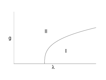
Figure 1: Phase diagram of graphene on the plane of $(\lambda,g)$. In region I, $m\neq 0$ and $\Gamma=0$. In region II, $m=0$ and $\Gamma\neq 0$ when $g\neq 0$. This phase diagram is valid for weak disorder.

In reality, the fermion gap $m(\mathbf{k})$ is not a constant, but is a function of fermion momentum. It is therefore essential to solve the equations (13) and (20) self-consistently. After carrying out extensive numerical computation at physical flavor $N=2$, we found a critical line on the plane of $(\lambda,g)$ and show the phase diagram in Fig.1. In region I with large $\lambda$ and small $g$, the dynamical fermion gap has a nontrivial solution, $m\neq 0$, but the disorder scattering rate have only trivial solution, $\Gamma=0$. In region II, the fermion gap has only trivial solution, $m=0$, while the disorder scattering rate acquires a finite value, $\Gamma\neq 0$ (certainly, $\Gamma$ vanishes when $g=0$). We did not find any evidence for the coexistence of nontrivial $m$ and nontrivial $\Gamma$ in numerical computation. The numerical results confirm our expectation that there is a competition between the generation of excitonic fermion gap and the generation of disorder scattering rate: fermion damping $\Gamma$ suppresses the formation of excitonic pairs, and fermion gap $m$ prevents the appearance of fermion damping.

In region I on Fig.1, the excitonic gap generation wins the competition, hence the ground state is an excitonic insulator with zero dc electric conductivity $\sigma=0$. In region II, the disorder scattering wins, then the ground state is gapless and the Dirac fermions acquire a finite scattering rate. In region II, the accurate calculation of electric conductivity is a problem in debate CastroNeto ; DasSarma . To the leading order of the Kubo formula, the dc electric conductivity is known to be $\sigma=4e^{2}/\pi h$, which is independent of disorder and universal Fradkin ; Lee93 ; Ando ; Mirlin ; Durst . When disorder strength $g$ grows from I to II, $\sigma$ jumps suddenly from zero to a universal value at certain critical value $g_{c}$. This is a first-order excitonic insulator to metal phase transition driven by growing disorder. Note, however, that the excitonic phase transition is of first-order only in the presence of finite disorder, $g\neq 0$. In the clean limit, $g=0$, the excitonic transition is not of first-order but is continuous as the Coulomb interaction parameter $\lambda$ is varied. There is indeed a debate on the nature of this transition in the clean graphene. An infinite-order transition was claimed in some theoretical analysis Gusynin ; Gamayun , whereas a conventional second-order transition was found in recent numerical work Drut09_1 .

As mentioned earlier, the disorder considered in this work is random chemical potential, which may be generated by local defects, neutral impurity atoms, or neutral adsorbed atoms in the plane of graphene Peres ; Mucciolo . When this type of disorder is smooth at the atomic scale, it will not mix the two inequivalent Dirac points. The parameter $g$ is indeed the product of the concentration of impurity atom (or defect) and the strength of a single impurity atom. In practice, the magnitude of the critical disorder parameter $g_{c}$ depends on the fermion flavor and the Coulomb interaction strength $\lambda$. If we take physical flavor $N=2$ and assume that graphene is suspended in vacuum so that $e^{2}/v_{F}\epsilon\approx 2.16$ CastroNetoPhysics , namely $\lambda\approx 13.57$, then it is easy to obtain $g_{c}\approx 0.36$. When graphene is placed on certain substrate, the Coulomb interaction strength is reduced by the screening due to substrate. From Fig. 1, we know that critical value $g_{c}$ decreases as $\lambda$ is lowered.

We would like to emphasize the importance of making a self-consistent analysis in our problem. In fact, if we solve the fermion gap function (13) by assuming a finite constant scattering rate $\Gamma$, then there is a critical value $\Gamma_{c}$. The gap equation has no nontrivial solution for $\Gamma>\Gamma_{c}$, but a finite fermion gap is opened for $\Gamma<\Gamma_{c}$. In this case, there is coexistence of finite fermion gap and finite scattering rate when $\Gamma<\Gamma_{c}$. Similarly, if we solve the SCBA equation (20) by assuming a free constant gap $m_{0}$, there will be coexistence of finite fermion gap and finite scattering rate when the inequality (22) is satisfied. In both these cases, there will be the third region with finite fermion gap $m$ and disorder scattering rate $\Gamma$ lying between region I and region II on the phase diagram. In this third region, the dc electric conductivity would be

$$\sigma=\frac{4e^{2}}{\pi h}\frac{\Gamma^{2}}{\Gamma^{2}+m^{2}},$$ (26)

which depends on disorder strength and displays metallic behavior even when the fermions are gapped. However, when the equations (13) and (20) are solved self-consistently, the fermion gap $m$ and scattering rate $\Gamma$ can not be finite simultaneously, and can not be zero simultaneously when $g\neq 0$. As a consequence, the dc electric conductivity is either zero or exactly quantized, and does not explicitly depend on disorder strength.

III Effect of additional four-fermion interaction

In additional to Coulomb interaction, the contact four-fermion interaction may also be important in realistic graphene. In the language of field theory, such contact interaction is normally described by the Gross-Neveu model Gross ; Rosenstein . It can make additional contributions to the generation of finite excitonic fermion gap Gross ; Rosenstein . A natural question is whether the contact interaction alters the phase diagram shown in Fig.1. When a four-fermion interaction is included in our self-consistent analysis, it is in principle possible to obtain a coexistence of finite excitonic fermion gap and finite scattering rate. In this section, we will examine this possibility.

As an concrete example, we consider the following Gross-Neveu model

$$H_{\mathrm{GN}}=\frac{G}{N}\sum_{\sigma=1}^{N}\int\left(\bar{\psi}_{\sigma}(\mathbf{r})\psi_{\sigma}(\mathbf{r})\right)^{2}.$$ (27)

This interaction term does not respect the continuous chiral symmetry, but respects a discrete chiral symmetry. Its role in excitonic gap generation was analyzed in recent years Herbut ; Hands ; Liu ; Gamayun . Unlike Coulomb interaction, the interaction strength does not depend on fermion momentum and energy and there is no dynamical or static screening.

We first ignore the Coulomb interaction and consider the Gross-Neveu model only. The corresponding gap equation is

$$m(\mathbf{p}) = \frac{g^{\prime}}{N\pi\Lambda}\int\frac{d^{2}\mathbf{k}}{(2\pi)^{2}}\frac{m(\mathbf{k})}{\sqrt{|\mathbf{k}|^{2}+m^{2}(\mathbf{k})}}$$ (28)

$$\times\mathrm{Im}\psi\left(\frac{1}{2}+\frac{\Gamma}{2\pi T}+i\frac{\sqrt{|\mathbf{k}|^{2}+m^{2}(\mathbf{k})}}{2\pi T}\right).$$

where $g^{\prime}=GN\Lambda$. From this equation, it is clear that fermion gap is indeed independent of momentum. At zero temperature, we can reduce gap equation to

$$1 = \frac{g^{\prime}}{2N\pi^{2}\Lambda}\int_{0}^{\Lambda}d|\mathbf{k}||\mathbf{k}|\frac{1}{\sqrt{|\mathbf{k}|^{2}+m^{2}}}\arctan\left(\frac{\sqrt{|\mathbf{k}|^{2}+m^{2}}}{\Gamma}\right).$$ (29)

In the clean limit, $\Gamma=0$, then

$$1 = \frac{g^{\prime}}{4N\pi\Lambda}\int_{0}^{\Lambda}d|\mathbf{k}||\mathbf{k}|\frac{1}{\sqrt{|\mathbf{k}|^{2}+m^{2}}},$$ (30)

which has solution

$$\frac{m}{\Lambda}=\frac{1-\left(\frac{4N\pi}{g^{\prime}}\right)^{2}}{\frac{8N\pi}{g^{\prime}}}.$$ (31)

There is a critical coupling $g^{\prime}_{c}=4N\pi$. When $g^{\prime}<g^{\prime}_{c}$, there is no non-trial solution for $m$; when $g^{\prime}>g^{\prime}_{c}$, there is non-trivial solution for $m$. In the presence of disorder, the scattering rate $\Gamma$ is given by the SCBA equation (20). Since now fermion gap $m$ is a constant, it is easy to obtain the following expression

$$\Gamma^{2}=\frac{\Lambda^{2}}{e^{4\pi/g}-1}-m^{2}.$$ (32)

After solving fermion gap equation (26) using this $\Gamma$, we found no coexistence of finite fermion gap and finite scattering rate.

We next consider the case when both Coulomb and Gross-Neveu interactions are present in graphene. Recently, Gamayun et al. showed that the analytical results can agree with numerical simulation results once the Gross-Neveu model is included Gamayun . Now the whole gap equation has the form

$$m(\mathbf{p}) = \int\frac{d^{2}\mathbf{k}}{4\pi^{2}}\frac{m(\mathbf{k})}{\sqrt{|\mathbf{k}|^{2}+m^{2}(\mathbf{k})}}\frac{1}{\frac{\mathbf{|p-k|}}{\lambda}+\Pi(0,\mathbf{p-k},\Gamma)}$$ (33)

$$\times\frac{1}{\pi}\arctan\left(\frac{\sqrt{|\mathbf{k}|^{2}+m^{2}(\mathbf{k})}}{\Gamma}\right)$$

$$+\frac{g^{\prime}}{N\Lambda}\int\frac{d^{2}\mathbf{k}}{4\pi^{2}}\frac{m(\mathbf{k})}{\sqrt{|\mathbf{k}|^{2}+m^{2}(\mathbf{k})}}\frac{1}{\pi}\arctan\left(\frac{\sqrt{|\mathbf{k}|^{2}+m^{2}(\mathbf{k})}}{\Gamma}\right),$$

which couples self-consistently to SCBA equation (20). After numerically solving these equations, we found no coexistence of finite fermion gap and finite scattering rate. Although the magnitude of fermion gap in the excitonic insulating phase becomes larger after Gross-Neveu interaction is included, the qualitative phase diagram shown in Fig.1 does not change.

IV Summary and discussion

In this paper, we studied the disorder effect on excitonic fermion gap generation, i.e., excitonic insulating transition, due to Coulomb interaction in graphene. By solving the self-consistent equations of fermion gap and disorder scattering rate, we found a strong competition between excitonic fermion gap generation and disorder scattering. As a consequence of this competition, fermion gap generation can not occur simultaneously with disorder scattering in graphene. The phase diagram presented in Fig.(1) is the main new output of this paper. We also showed that this phase diagram is not changed by additional contact four-fermion interaction.

In any realistic graphene, the Dirac fermions are always scattered by some kinds of disorder. Our results indicate that, even if the Coulomb interaction is indeed sufficiently strong, the excitonic transition will be completely suppressed if the disorder strength is not small enough. Apparently, the excitonic transition can most possibly be observed in very clean graphene.

We would point out that our results are obtained using SCBA. It would be interesting to examine the effect of higher order corrections. The most important corrections come from the fluctuation effect associated with the Anderson localization. When $\Gamma\neq 0$, the metallic electric conductivity $\sigma=4e^{2}/\pi h$ is subjected to diffusion and Cooperon vertex corrections Lee85 , which will lead to Anderson metal-insulator transition. When Coulomb interaction is absent, $\lambda=0$, the localization of massless Dirac fermions was found Aleiner ; Altland . For small but finite $\lambda$, though Coulomb interaction is not strong enough to open fermion gap, it can have important influence on transport properties Kotov ; Khveshchenko06 ; Mishchenko ; Schmalian ; Mishchenkoepl ; Herbut2008 ; Muller ; Herbut2010 . In particular, it may destroy the fermion localization Abrahams . However, there is currently no widely accepted theory for the interaction effect on localization Abrahams . On the experimental side, earlier measurements suggested that the undoped graphene exhibits a universal minimum conductivity CastroNeto , $\sigma=4e^{2}/h$. More recently, it becomes clear from extensive transport experiments that the minimum conductivity in undoped graphene is not universal but instead strongly sample-dependent Mucciolo ; Tan ; ChenNP ; ChenPRL . Regardless of the precise value of minimum conductivity, it seems that the undoped, gapless graphene is metallic and free of localization at experimentally accessible temperature DasSarma ; Peres ; Mucciolo , at least for weak disorder.

In this paper, we are mainly interested in the regime of strong Coulomb interaction. For large $\lambda$, the localization effect is even more involved because it is entangled with the non-perturbative phenomenon of excitonic gap generation. As already explained, a self-consistent treatment is crucial in our problem, hence excitonic gap generation and fermion localization can not be studied separately. Technically, the fermion gap function $m(\mathbf{p})$ appearing in (13) should be used when computing the diffusion and Cooperon vertex corrections, while these vertex corrections should be included in the polarization function $\Pi(\mathbf{p})$ and the fermion gap equation (13), which correspond to the Altshuler-Aronov type corrections Lee85 . Unfortunately, although in principle it is possible to examine the importance of Anderson localization effect, the self-consistent equations obtained in this way are too complicated to be analyzed theoretically or numerically.

In this paper, we considered only one particular type of disorder, i.e., random chemical potential. Our self-consistent analysis may be extended to study the effects of other types of disorders Ludwig , such as random gauge field or random mass, on excitonic pairing formation. Specifically, ripples are believed by many people to be important in graphene and thus attracted intensive investigation Guinea . Such ripple configuration can be described by a random gauge potential Guinea . It is interesting to study the ripple effect and to examine whether ripples can drive an analogous phase transition in the future.

We would like to thank P. Pyatkovskiy for pointing out a mistake in our previous calculation of polarization function and W. Li and J. Wang for helpful discussion. G.Z.L. is supported by the National Science Foundation of China under Grant No.11074234 and the project sponsored by the Overseas Academic Training Funds of University of Science and Technology of China.

References

References

- (1) A. H. Castro Neto, F. Guinea, N. M. R. Peres, K. S. Novoselov, and A. K. Geim, Rev. Mod. Phys. 81, 109 (2009).
- (2) S. Das Sarma, S. Adam, E. H. Hwang, and E. Rossi, arXiv:1003.4731v2.
- (3) N. M. R. Peres, Rev. Mod. Phys. 82, 2673 (2010).
- (4) E. R. Mucciolo and C. H. Lewenkopf, J. Phys.: Condens. Matter 22, 273201 (2010).
- (5) D. S. L. Abergel, V. Apalkov, J. Berashevich, K. Ziegler, and T. Chakraborty, Adv. Phys. 59, 261 (2010).
- (6) V. N. Kotov, B. Uchoa, V. M. Pereira, A. H. Castro Neto, and F. Guinea, arXiv:1012.3484v1.
- (7) J. Gonzalez, F. Guinea, and M. A. H. Vozmediano, Nucl. Phys. B 424, 595 (1994).
- (8) D. V. Khveshchenko, Phys. Rev. Lett. 87, 246802 (2001).
- (9) D. V. Khveshchenko and H. Leal, Nucl. Phys. B 687, 323 (2004).
- (10) E. V. Gorbar, V. P. Gusynin, V. A. Miransky, and I. A. Shovkovy, Phys. Rev. B 66, 045108 (2002).
- (11) I. F. Herbut, Phys. Rev. Lett. 97, 146401 (2006).
- (12) S. J. Hands and C. G. Strouthos, Phys. Rev. B 78, 165423 (2008).
- (13) J. E. Drut and T. A. Lahde, Phys. Rev. Lett. 102, 026802 (2009).
- (14) J. E. Drut and T. A. Lahde, Phys. Rev. B 79, 165425 (2009).
- (15) G.-Z. Liu, W. Li, and G. Cheng, Phys. Rev. B 79, 205429 (2009).
- (16) O. V. Gamayun, E. V. Gorbar, and V. P. Gusynin, Phys. Rev. B 81, 075429 (2010).
- (17) A. Durst and P. A. Lee, Phys. Rev. B 62, 1270 (2000).
- (18) E. Fradkin, Phys. Rev. B 33, 3263 (1986).
- (19) P. A. Lee, Phys. Rev. Lett. 71, 1887 (1993).
- (20) Y. Zheng and T. Ando, Phys. Rev. B 65, 245420 (2002).
- (21) P. M. Ostrovsky, I. V. Gornyi, and A. D. Mirlin, Phys. Rev. B 74, 235443 (2006).
- (22) I. L. Aleiner and K. B. Efetov, Phys. Rev. Lett. 97, 236801 (2006).
- (23) A. H. Castro Neto, Physics 2, 30 (2009).
- (24) D. J. Gross and A. Neveu, Phys. Rev. D 10, 3235 (1974).
- (25) B. Rosenstein, B. J. Warr, and S. H. Park, Phys. Rep. 205, 59 (1991).
- (26) P. A. Lee and T. V. Ramakrishnan, Rev. Mod. Phys. 57, 287 (1985).
- (27) A. Altland, Phys. Rev. Lett. 97, 236802 (2006).
- (28) D. V. Khveshchenko, Phys. Rev. B 74, 161402(R) (2006).
- (29) E. G. Mishchenko, Phys. Rev. Lett. 98, 216801 (2007).
- (30) D. E. Sheehy and J. Schmalian, Phys. Rev. Lett. 99, 226803 (2007).
- (31) E. G. Mishchenko, Europhys. Lett. 83, 17005 (2008).
- (32) I. F. Herbut, V. Juricic, and O. Vafek, Phys. Rev. Lett. 100, 046403 (2008).
- (33) M. Muller, J. Schmalian, and L. Fritz, Phys. Rev. Lett. 103, 025301 (2009).
- (34) V. Juricic, O. Vafek, and I. F. Herbut, Phys. Rev. B 82, 235402 (2010).
- (35) E. Abrahams, S. V. Kravchenko, and M. P. Sarachik, Rev. Mod. Phys. 73, 251 (2001).
- (36) Y. W. Tan, Y. Zhang, K. Bolotin, Y. Zhao, S. Adam, E. H. Hwang, S. Das Sarma, H. L. Stormer, and P. Kim, Phys. Rev. Lett. 99, 246803 (2007).
- (37) J. H. Chen, C. Jang, S. Adam, M. S. Fuhrer, E. D. Williams, and M. Ishigami, Nat. Phys. 4, 377 (2008).
- (38) J. H. Chen, W. G. Cullen, C. Jang, M. S. Fuhrer, and E. D. M. Williams, Phys. Rev. Lett. 102, 236805 (2009).
- (39) A. W. W. Ludwig, M. P. A. Fisher, R. Shankar, and G. Grinstein, Phys. Rev. B 50, 7526 (1994).
- (40) M. A. J. Vozmediano, M. I. Katsnelson, and F. Guinea, Phys. Rep. 496, 109 (2010).