Very Large Telescope Kinematics for omega Centauri: Further Support for a Central Black Hole.

Abstract

The Galactic globular cluster $\omega$ Centauri is a prime candidate for hosting an intermediate mass black hole. Recent measurements lead to contradictory conclusions on this issue. We use VLT-FLAMES to obtain new integrated spectra for the central region of $\omega$ Centauri. We combine these data with existing measurements of the radial velocity dispersion profile taking into account a new derived center from kinematics and two different centers from the literature. The data support previous measurements performed for a smaller field of view and show a discrepancy with the results from a large proper motion data set. We see a rise in the radial velocity dispersion in the central region to 22.8$\pm$1.2 $\rm{km}~{}\rm s^{-1}$, which provides a strong sign for a central black hole. Isotropic dynamical models for $\omega$ Centauri imply black hole masses ranging from $3.0$ to $5.2\times 10^{4}M_{\odot}$ depending on the center. The best-fitted mass is $(4.7\pm 1.0)\times 10^{4}M_{\odot}$.

1. Introduction

Intermediate-mass black holes (IMBHs) may bridge the gap between stellar mass black holes and super-massive black holes found in the center of most galaxies. Their existence is appealing in various ways: they could extend the $M_{\bullet}-\sigma$ relation for galaxies (Gebhardt et al., 2000a; Ferrarese & Merritt, 2000) down to dwarf galaxies and globular clusters, and present a potential connection to nuclear star clusters (Seth et al., 2010). They could also be the seeds for super-massive black holes and alleviate problems with difficulties to account for the rapid growth necessary to explain massive QSOs at high redshift (Tanaka & Haiman, 2009).

The existence of an IMBH at the center of $\omega$ Centauri (NGC 5139) has been controversial. Noyola et al. (2008) (hereafter NGB08) obtain line-of-sight velocity dispersion (LOSVD) measurements using the Gemini-GMOS integral field unit (IFU). They find a velocity dispersion rise toward the center implying the presence of a $(4\pm 1)\times 10^{4}M_{\odot}$ black hole when compared to spherical isotropic dynamical models. In contrast, van der Marel & Anderson (2010) (hereafter vdMA10), using proper motions from HST-ACS imaging, find a lower black hole mass of $(1.8\pm 0.3)\times 10^{4}M_{\odot}$ for an isotropic model and their profile with a central cusp. Their anisotropic model sets an upper limit of $7.4\times 10^{3}M_{\odot}$. The comparison is complicated by the fact that the cluster centers between NGB08 and Anderson & van der Marel (2010) (hereafter AvdM10) are separated by $\sim 12\arcsec$.

The nature of $\omega$ Centauri has been under discussion for a while. This object has been regarded as the largest globular cluster in the Galactic system, but the clear metallicity spread (Norris et al., 1996; Sollima et al., 2005), as well as a double main sequence (Bedin et al., 2004; Piotto et al., 2005) has led to the suggestion that it might be the stripped core of a dwarf galaxy (Freeman, 1993; Meza et al., 2005; Bekki & Norris, 2006). $\omega$ Cen has a large central velocity dispersion of $22\pm 4$ $\rm{km}~{}\rm s^{-1}$ (Meylan et al., 1995), as well as a fast global rotation of 8 $\rm{km}~{}\rm s^{-1}$ (Merritt et al., 1997), at 11 pc from the center. It is the most flattened Galactic globular cluster (White & Shawl, 1987), and has a retrograde orbit around the galaxy (Dinescu et al., 2001). Using both radial velocities and proper motions van de Ven et al. (2006) calculate a total mass of $2.5\times 10^{6}M_{\odot}$, making $\omega$ Cen the most massive Galactic globular cluster.

The extrapolation of the $M_{\bullet}-\sigma$ relation for galaxies (Tremaine et al., 2002) predicts a $1.3\times 10^{4}M_{\odot}$ black hole for $\omega$ Cen. At a distance of $4.8\pm 0.3$ kpc (van de Ven et al., 2006), the sphere of influence of such a black hole is $\sim$ 5″. In this Letter, we present new VLT-ARGUS data that we compare to previous measurements.

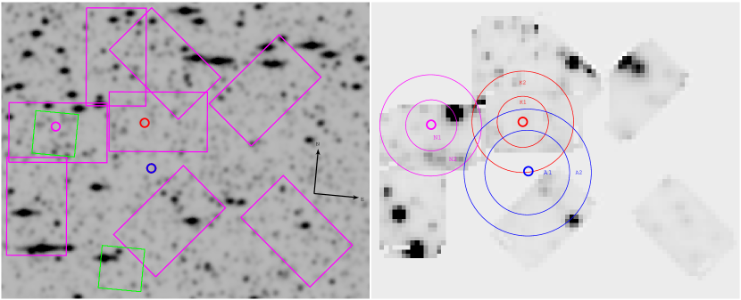
Figure 1.— Left: Area of the eight pointings observed with ARGUS overlaid on a convolved HST-ACS image of $\omega$ Centauri (about 30″$\times$ 40″). The two explored centers (magenta circle: NGB08, blue circle: AvdM10), the new kinematic center (red), and the previous GMOS IFU pointings (green squares) are marked for comparison. Right: reconstructed ARGUS images for the eight pointings. The overlaid circles show the two central annuli in which the velocity dispersion is measured as a function of radius.

2. Observations and Data Reduction

We obtain central kinematics data of $\omega$ Cen using the ARGUS IFU with FLAMES on the Very Large Telescope (VLT). With a central $\sigma$ around 20 $\rm{km}~{}\rm s^{-1}$, a spectral resolving power of $R\sim$10,000 is sufficient to measure the dispersion from integrated stellar light. The Ca-triplet region (8450–8700Å) is well suited for kinematic analysis. The LR8 setup of the GIRAFFE spectrograph (Pasquini et al., 2002), covering the range 820–940 nm at $R\sim$10,400 in ARGUS mode, is ideally suited for our study.

The ARGUS IFU was used in the 1:1 magnification mode providing a field of view of 11.5″$\times$7.3″, sampled by 0.52″$\times$0.52″pixels. The FLAMES observations were taken during two nights (2009 June 15 and 16). Eight different pointings were obtained at and around the two contended center determinations (see Figure 1). While the pointings aimed at including both centers, position inaccuracies in the guide star catalogs made us miss the second from AvdM10. The final set of observations consists of three exposures for the first ARGUS pointings (around the NGB08 center) and two exposures for the seven other pointings, with exposure times of 1500s for the first two, 1020s for the next two (90^∘ tilted, see Fig. 1) and 900s for the four peripheral pointings ($\pm$45^∘ tilted).

The first reduction steps are done with the GIRAFFE pipeline (based on the Base Line Data Reduction Software developed by the Observatoire de Genève). The pipeline recipes gimasterbias, gimasterdark, gimasterflat and giscience produce bias corrected, dark subtracted, fiber-to-fiber transmission and pixel-to-pixel variations corrected spectra. Sky subtraction and wavelength calibration are performed with our own tools, which test the wavelength solution with arc exposures and skylines.

We reconstruct the ARGUS data cubes to images in order to determine the exact location of the pointings with respect to reference Hubble Space Telescope (HST) images. We use a large Advanced Camera for Surveys (ACS) mosaic of $\omega$ Cen (GO-9442, PI: A. Cool), which we convolve to ground-based observed spatial resolution. The reconstructed ARGUS images are matched to the convolved ACS image and used to assign the correct location and position angle from both centers to each pixel and to identify pixels which are dominated by single stars (i.e., not suited to derive a velocity dispersion).

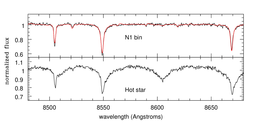
Figure 2.— Examples of integrated spectra for the N1 bin (top), as well as for one of the hot stars (bottom). The black line shows the combined spectra, and the red line shows the fit used for kinematics

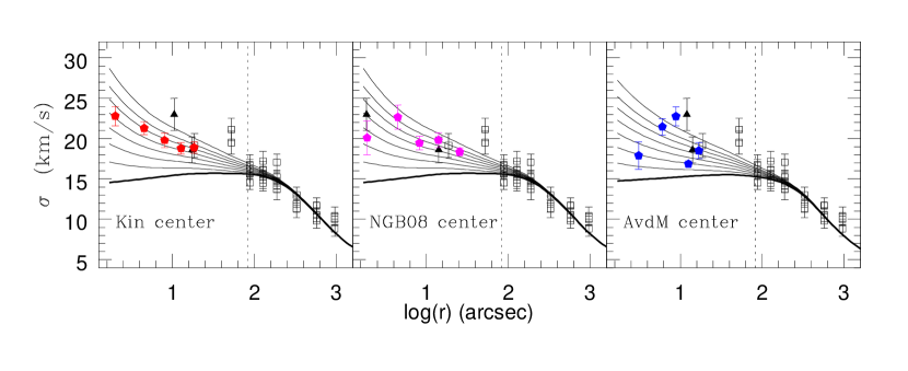
Figure 3.— Velocity dispersion as a function of radius. The dashed line marks the core radius. The open squares are measurements taken from van de Ven et al. (2006). The solid lines show isotropic spherical models assuming various black holes masses (0,1,2,3,4,5,6, and 7.5$\times 10^{4}~{}M_{\odot}$). The left panel shows the measured $\sigma$ assuming the new kinematic center (filled red pentagons), while the middle and right panels show the same for the NGB08and AvdM10 center. Black triangles mark the kinematic measurements from NGB08.

3. Kinematic Measurements

Measuring kinematics of globular clusters from integral field spectroscopy is challenging. For details, we refer to NGB08. A key aspect to consider is the fact that bright stars might dominate the integrated light and increase the shot noise of the velocity dispersion . In order to minimize the shot noise from bright stars, we can choose which pixels to combine for the integrated light measure of the velocity dispersion.

There are hot stars with strong Paschen-series lines present (see Fig 2). We exclude regions dominated by these stars and those dominated by bright stars. We identify these regions by including one of these stars in the velocity template library and then exclude those regions which have a significant contribution, $\sim$5% of the pixels are excluded in this way. We also exclude those regions dominated by bright stars. After these two cuts, about 85% of the pixels remain to derive kinematics. To further minimize the effect from bright stars, we divide each spectrum by its mean value, thereby giving all pixels equal weight when combining..

We consider the shot noise from having a small number of stars contribute to a spatial bin. We calculate the shot noise using the HST $R$-band photometry from AvdM10. We use Monte Carlo simulations to generate a mock velocity data set in a given spatial bin, using magnitudes of present stars. We then estimate a velocity dispersion weighted by the fluxes of the stars. After 1000 realizations, we get sample velocity dispersion estimates from which we obtain the scatter, and hence the shot noise.

We rely on both centers by NGB08 and AvdM10, which differ by 12″. AvdM10 claim that the center of NGB08 is biased toward bright stars and that these stars do not trace the center well. On the other hand, using corrected star counts biases one away from bright stars. Thus, there may be reasons to expect increased noise for the center position in both techniques. Given that we have two-dimensional (2D) kinematics, we can provide another center based on kinematics by running a kernel of 5″ across the field and estimating the velocity dispersion within that kernel. From the 2D dispersion map there is a clear peak at the location highlighted in Fig. 2. It lies about 10″from NGB08 and 3.5″ from AvdM10. We make dynamical models using the three centers.

We use five annuli centered on each center for the dynamical analysis. We combine the pixels within each annulus using a biweight estimator (Beers et al., 1990). The average radius of the annuli are given in Table 1, they are chosen to provide a signal-to-noise ratio of at least 40 in each bin. The central annulus has about 60 pixels and the outer has 500. The shot noise in any of the outer annuli is below 3% of the velocity dispersion. In the central bins, the shot noise is 3% for the kinematic center, 6% for AvdM10 and 9% for NGB08. The uncertainties in Table 1 include the shot noise added in quadrature with the measured uncertainties.

In order to extract the kinematics from the spectra, we use the technique described in Gebhardt et al. (2000b) and Pinkney et al. (2003), also employed in NGB08. This technique provides a non-parametric estimate of the LOSVD. Starting from velocity bins of 8 $\rm{km}~{}\rm s^{-1}$, we adjust the height of each LOSVD bin to define a sample LOSVD. This LOSVD is convolved with a template. The parameters, bin heights and template mix are changed to minimize the $\chi^{2}$ fitted with the data spectrum. For the template, we use two individual stars within the IFU; these are a normal late-type giant star, and a hot star (shown in Fig. 2). The program then determines the relative weight of these two stars.

Table 1Velocity measurements.

Bin	$R$	$V$	$\Delta V$	$\sigma$	$\Delta\sigma$	$h_{3}$	$\Delta h_{3}$	$h_{4}$	$\Delta h_{4}$
	″	$km/s$	$km/s$	$km/s$	$km/s$
K1	2.0	1.1	0.5	22.8	1.2	0.05	0.03	-0.05	0.01
K2	4.5	-1.1	0.4	21.3	0.8	0.03	0.03	-0.05	0.01
K3	8.0	3.0	0.4	19.8	0.9	0.01	0.03	-0.04	0.01
K4	12.7	2.3	0.4	18.8	0.7	-0.01	0.02	-0.04	0.01
K5	18.3	1.9	0.4	18.9	0.7	-0.00	0.03	-0.05	0.01
N1	1.9	-0.6	0.4	20.1	2.1	0.00	0.02	-0.05	0.01
N2	4.5	1.4	0.5	22.7	1.5	-0.01	0.04	-0.06	0.01
N3	8.2	1.3	0.4	19.5	0.8	-0.01	0.04	-0.05	0.01
N4	14.0	1.0	0.4	19.8	0.9	0.01	0.03	-0.04	0.01
N5	25.5	3.9	0.4	18.4	0.5	0.01	0.03	-0.05	0.01
A1	3.1	8.7	0.3	17.9	1.7	0.01	0.03	-0.04	0.01
A2	6.0	-2.2	0.4	21.5	1.0	0.05	0.03	-0.05	0.01
A3	8.8	-0.5	0.5	22.8	1.2	0.00	0.03	-0.08	0.01
A4	12.6	4.2	0.4	16.9	0.4	0.03	0.02	-0.06	0.01
A5	16.9	0.6	0.4	18.5	1.0	-0.01	0.04	-0.04	0.01

The non-parametric LOSVD estimate requires a smoothing parameter (see Gebhardt et al. (2000b) for a discussion) in order to produce a realistic profile, otherwise, adjacent velocity bins can show large variations. We use the smallest smoothing value just before the noise in the LOSVD bins becomes large (similar to a cross-validation technique). In addition to a non-parametric estimate, we fit a Gaussian–Hermite profile including the first four moments. The second moment of both the Gauss–Hermite profile and the non-parametric LOSVD is similar, which implies that we have a good estimate for the smoothing value. We first fit all individual 4700 pixels in all dithered positions of the IFU. This step allows us to identify those pixels where hot stars provide a significant contribution. We then exclude those pixels from the combined spectra. The top spectrum in Fig. 2 shows the spectral fit to the central radial bin.

The uncertainties for the LOSVD come from Monte Carlo simulations. For each spectrum, we generate a set of realizations from the best-fitted spectrum (template convolved with the LOSVD), and add noise according to the rms of the fit. We then fit a new LOSVD, varying the template mix. From the run of realizations we take the 68% confidence band to determine the LOSVD uncertainties.

Given that $\omega$ Cen contains stars with different spectral types, we also allow the equivalent widths to be an additional parameter. This parameter allows for mismatch between the stars chosen as templates and different regions of the cluster. We have tried a variety of different template stars and find no significant changes. Table 1 presents the first four moments ($v$, $\sigma$, $h_{3}$, and $h_{4}$) of a Gauss-Hermite expansion fitted to the non-parametric LOSVD. We note that the LOSVDs have statistically-significant non-zero $h_{4}$ components, which are important for the dynamical modeling in terms of constraining the stellar orbital properties.

Fig. 3 shows velocity dispersions from the LOSVDs for spectra combined around all centers. Every case shows an increase in the dispersion compared to data outside 50″, while isotropic models without a black hole expect a drop in the central velocity dispersion. The dispersion profile obtained for the kinematic center shows a smooth rise, the one for the NGB08 center is still relatively smooth, while the profile for the AvdM10 center shows larger variation. While the larger scatter is not evidence that the two previous centers are not proper, it is suggestive.

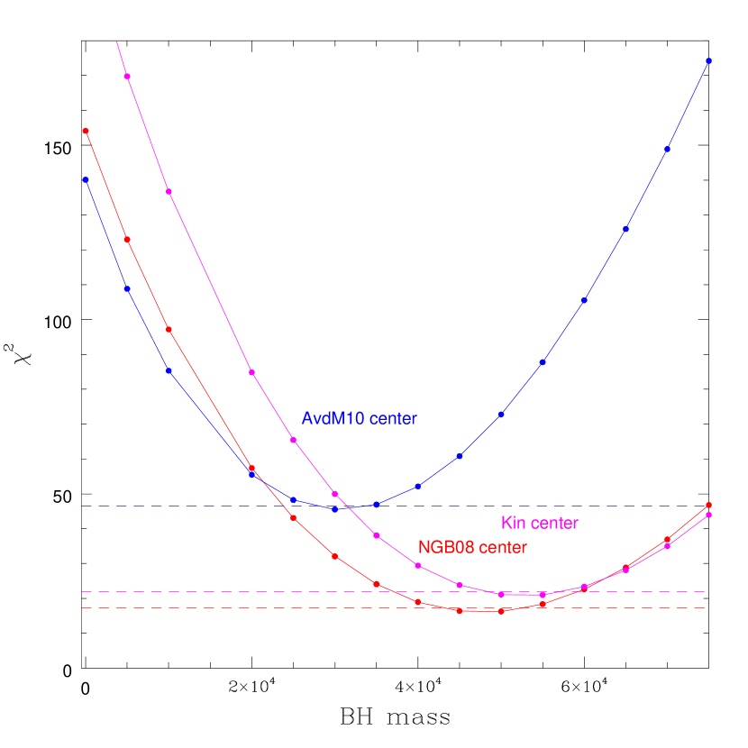
Figure 4.— $\chi^{2}$ for our isotropic, spherical model fits to the data, shown for the three cases: the kinematic center (magenta curve) the AvdM10 center [blue curve], and the NGB08 ( red curve). In both cases the best fit is obtained with a black hole of a few $10^{4}~{}M_{\odot}$, while a better fit is achieved assuming our original center.

4. Isotropic Models and Discussion

A detailed comparison with N-body simulations and orbit based models is in preparation. These models will also consider possible velocity anisotropy and contribution of dark remnants, as well as include a comparison with the large proper motion dataset in AvdM10. For the scope of this Letter, we limit ourselves to a comparison of the present data with isotropic models. These models have represented the projected quantities for globular clusters extremely well, starting with King (1966) all the way to a recent analysis by McLaughlin et al. (2006), where the conclusion is that clusters are isotropic within their core. Thus, while isotropy needs to be explored in detail, it provides a very good basis for comparison.

For the details of the isotropic analysis, we refer to NGB08, essentially following the non-parametric method described in Gebhardt & Fischer (1995). The surface brightness profile is the one obtained in NGB08, which is smoothed and deprojected assuming spherical symmetry in order to obtain a luminosity density profile (Gebhardt et al., 1996). By assuming an $M/L$ ratio, we calculate a mass density profile, from which the potential and the velocity dispersion can be derived. We repeat the calculation adding various central point masses ranging from 0 to $7.5\times 10^{4}M_{\odot}$ while keeping the global $M/L$ value fixed. Since vdMA10 obtain a density profile from star counts, we use their Nuker fit to the star-count profile to create a similar set of models. We note that the $M/L$ value needed to fit the kinematics outside the core radius is 2.7 for both profiles. For comparison, van de Ven et al. (2006) found an $M/L$ value of 2.5.

Binaries could potentially bias a velocity dispersion measured from radial velocities, which is not an issue for proper motions. Carney et al. (2005) estimate an 18% binary fraction for $\omega$ Cen (with large uncertainties); this implies that at any given time, the observed fraction is about a few percent due to chance inclination and phase (Hut et al., 1992). Also, Ferraro et al. (2006) find no mass segregation for this cluster tracing the blue straggler population with radius. Both facts imply that the expected binary contamination is low (a few percent), which at most would cause a few percent increase in the measured velocity dispersion (i.e., within our errors).

Figure 3 shows the comparison between the different models and the measured dispersion profiles. As in our previous study, the most relevant part of the comparison is the rise inside the core radius. As can be seen, an isotropic model with no black hole predicts a slight decline in the velocity dispersion toward the center which is not observed for any of the assumed centers. The calculated $\chi^{2}$ values for each model are plotted in Fig. 4, as well as a line showing $\Delta\chi^{2}=1$. The $\chi^{2}$ curve implies a best-fitted black hole mass of several $10^{4}M_{\odot}$ in every case, but with lower $\chi^{2}$ for the NGB08 center. Specifically, a black hole of mass of $(5.2\pm 0.5)\times 10^{4}M_{\odot}$ is found for the kinematic center $(4.75\pm 0.75)\times 10^{4}M_{\odot}$ for the NGB08 center, and of $(3.0\pm 0.4)\times 10^{4}M_{\odot}$ for the AvdM10 center.

The velocity dispersion at 100″ is well measured at around 17 $\rm{km}~{}\rm s^{-1}$. The radial velocities inward show a continual rise in the dispersion with smaller radii to the central value around 22.8 $\rm{km}~{}\rm s^{-1}$, which is statistically significant. This rise is now seen in multiple radial velocity datasets. It is this gradual rise that provides the significance for a central black hole. The proper motion data of AvdM10 show a slight rise in the velocity dispersion, but not all the way into their center. It is unclear why the two dispersion measurements differ.

References

- Anderson & van der Marel (2010) Anderson, J., & van der Marel, R. P. 2010, ApJ, 710, 1032
- Bedin et al. (2004) Bedin, L. R., Piotto, G., Anderson, J., Cassisi, S., King, I. R., Momany, Y., & Carraro, G. 2004, ApJL, 605, L125
- Beers et al. (1990) Beers, T. C., Flynn, K., & Gebhardt, K. 1990, AJ, 100, 32
- Bekki & Norris (2006) Bekki, K., & Norris, J. E. 2006, ApJ, 637, L109
- Carney et al. (2005) Carney, B. W., Aguilar, L. A., Latham, D. W., & Laird, J. B. 2005, AJ, 129, 1886
- Dinescu et al. (2001) Dinescu, D. I., Majewski, S. R., Girard, T. M., & Cudworth, K. M. 2001, AJ, 122, 1916
- Ferrarese & Merritt (2000) Ferrarese, L., & Merritt, D. 2000, ApJL, 539, L9
- Ferraro et al. (2006) Ferraro, F. R., Sollima, A., Rood, R. T., Origlia, L., Pancino, E., & Bellazzini, M. 2006, ApJ, 638, 433
- Freeman (1993) Freeman, K. C. 1993, in ASP Conf. Ser. 48: The Globular Cluster-Galaxy Connection, 608–+
- Gebhardt & Fischer (1995) Gebhardt, K., & Fischer, P. 1995, AJ, 109, 209
- Gebhardt et al. (1996) Gebhardt, K., et al. 1996, AJ, 112, 105
- Gebhardt et al. (2000a) —. 2000a, ApJ, 539, L13
- Gebhardt et al. (2000b) —. 2000b, AJ, 119, 1157
- Hut et al. (1992) Hut, P., et al. 1992, PASP, 104, 981
- King (1966) King, I. R. 1966, AJ, 71, 64
- McLaughlin et al. (2006) McLaughlin, D. E., et al. 2006, ApJS, 166, 249
- Merritt et al. (1997) Merritt, D., Meylan, G., & Mayor, M. 1997, AJ, 114, 1074
- Meylan et al. (1995) Meylan, G., Mayor, M., Duquennoy, A., & Dubath, P. 1995, A&A, 303, 761
- Meza et al. (2005) Meza, A., Navarro, J. F., Abadi, M. G., & Steinmetz, M. 2005, MNRAS, 359, 93
- Norris et al. (1996) Norris, J. E., Freeman, K. C., & Mighell, K. J. 1996, ApJ, 462, 241
- Noyola et al. (2008) Noyola, E., Gebhardt, K., & Bergmann, M. 2008, ApJ, 676, 1008
- Pasquini et al. (2002) Pasquini, L., et al. 2002, The Messenger, 110, 1
- Pinkney et al. (2003) Pinkney, J., et al. 2003, ApJ, 596, 903
- Piotto et al. (2005) Piotto, G., et al. 2005, ApJ, 621, 777
- Seth et al. (2010) Seth, A. C., et al. 2010, ApJ, 714, 713
- Sollima et al. (2005) Sollima, A., Pancino, E., Ferraro, F. R., Bellazzini, M., Straniero, O., & Pasquini, L. 2005, ApJ, 634, 332
- Tanaka & Haiman (2009) Tanaka, T., & Haiman, Z. 2009, ApJ, 696, 1798
- Tremaine et al. (2002) Tremaine, S., et al. 2002, ApJ, 574, 740
- van de Ven et al. (2006) van de Ven, G., van den Bosch, R. C. E., Verolme, E. K., & de Zeeuw, P. T. 2006, A&A, 445, 513
- van der Marel & Anderson (2010) van der Marel, R. P., & Anderson, J. 2010, ApJ, 710, 1063
- White & Shawl (1987) White, R. E., & Shawl, S. J. 1987, ApJ, 317, 246