11email: ncrocket@umich.edu 22institutetext: California Institute of Technology, Cahill Center for Astronomy and Astrophysics 301-17, Pasadena, CA 91125 USA 33institutetext: Department of Physics and Astronomy, Johns Hopkins University, 3400 North Charles Street, Baltimore, MD 21218, USA 44institutetext: Centre d’étude Spatiale des Rayonnements, Université de Toulouse [UPS], 31062 Toulouse Cedex 9, France 55institutetext: CNRS/INSU, UMR 5187, 9 avenue du Colonel Roche, 31028 Toulouse Cedex 4, France 66institutetext: Laboratoire d’Astrophysique de l’Observatoire de Grenoble, BP 53, 38041 Grenoble, Cedex 9, France. 77institutetext: Centro de Astrobiología (CSIC/INTA), Laboratiorio de Astrofísica Molecular, Ctra. de Torrejón a Ajalvir, km 4 28850, Torrejón de Ardoz, Madrid, Spain 88institutetext: Max-Planck-Institut für Radioastronomie, Auf dem Hügel 69, 53121 Bonn, Germany 99institutetext: LERMA, CNRS UMR8112, Observatoire de Paris and École Normale Supérieure, 24 Rue Lhomond, 75231 Paris Cedex 05, France 1010institutetext: LPMAA, UMR7092, Université Pierre et Marie Curie, Paris, France 1111institutetext: LUTH, UMR8102, Observatoire de Paris, Meudon, France 1212institutetext: I. Physikalisches Institut, Universität zu Köln, Zülpicher Str. 77, 50937 Köln, Germany 1313institutetext: Jet Propulsion Laboratory, Caltech, Pasadena, CA 91109, USA 1414institutetext: Departments of Physics, Astronomy and Chemistry, Ohio State University, Columbus, OH 43210, USA 1515institutetext: National Research Council Canada, Herzberg Institute of Astrophysics, 5071 West Saanich Road, Victoria, BC V9E 2E7, Canada 1616institutetext: Infrared Processing and Analysis Center, California Institute of Technology, MS 100-22, Pasadena, CA 91125 1717institutetext: Canadian Institute for Theoretical Astrophysics, University of Toronto, 60 St George St, Toronto, ON M5S 3H8, Canada 1818institutetext: Harvard-Smithsonian Center for Astrophysics, 60 Garden Street, Cambridge MA 02138, USA 1919institutetext: National University of Ireland Maynooth. Ireland 2020institutetext: SRON Netherlands Institute for Space Research, PO Box 800, 9700 AV, Groningen, The Netherlands 2121institutetext: Department of Physics and Astronomy, University of Calgary, 2500 University Drive NW, Calgary, AB T2N 1N4, Canada 2222institutetext: MPI für Sonnensystemforschung, D 37191 Katlenburg-Lindau, Germany 2323institutetext: Leiden Observatory, Leiden University, PO Box 9513, NL-2300 RA Leiden, The Netherlands 2424institutetext: LERMA & UMR8112 du CNRS, Observatoire de Paris, 61, Av. de l’Observatoire, 75014 Paris, France 2525institutetext: LERMA, CNRS UMR8112, Observatoire de Paris and École Normale Supérieure, 24 Rue Lhomond, 75231 Paris Cedex 05, France
Herschel observations of EXtra-Ordinary Sources: The Terahertz spectrum of Orion KL seen at high spectral resolution††thanks: Herschel is an ESA space observatory with science instruments provided by European-led Principal Investigator consortia and with important participation from NASA.
We present the first high spectral resolution observations of Orion KL in the frequency ranges 1573.4 – 1702.8 GHz (bands 6b) and 1788.4 – 1906.8 GHz (band 7b) obtained using the HIFI instrument on board the Herschel Space Observatory. We characterize the main emission lines found in the spectrum, which primarily arise from a range of components associated with Orion KL including the hot core, but also see widespread emission from components associated with molecular outflows traced by H2O, SO2, and OH. We find that the density of observed emission lines is significantly diminished in these bands compared to lower frequency Herschel/HIFI bands.
Key Words.:
Astrochemistry — ISM: general — ISM: clouds — ISM: molecules — Submillimeter: ISM1 Introduction
The Kleinmann-Low nebula within the Orion molecular cloud (Orion KL) is the best studied massive star forming region in the Milky Way. This region is characterized by a high IR luminosity (Kleinmann & Low, 1967) and rich molecular line emission. As such, it has been the subject of numerous molecular line surveys in the millimeter and submillimeter that have characterized its mm/sub-mm wave spectrum (see e.g. Schilke et al., 1997; Comito et al., 2005; Tercero et al., 2010, and references therein). These surveys reveal the presence of a prodigious variety of molecular species in addition to several distinct spatial/velocity components (i.e. the hot core, compact ridge, plateau, and extended ridge; Blake et al., 1987; Persson et al., 2007). These observations provide insight into the complex chemical and physical processes that characterize how massive stars form and interact with their natal environment. Because Orion KL is the closest such massive star forming region (414 pc; Menten et al. 2007), it is an ideal choice for further inquiry in understanding the chemistry and physics of the gas in close proximity to these stars.
Although the subject of much spectroscopic study in the mm /sub-mm ( 300m) during the past 30 years, high resolution observations at Terahertz (THz) frequencies of Orion KL have been unavailable from the ground due to atmospheric absorption. ISO provided the first comprehensive spectroscopic view of Orion KL at these wavelengths. Lerate et al. (2006) presented spectroscopic observations in the wavelength range 44 – 188 m (1.6 – 6.8 THz) with a resolving power of 6800-9700 using the long wavelength spectrometer (LWS) on board ISO. These data showed a spectrum dominated by emission from H2O, OH, and CO, but little or no emission from more complex species (such as methanol, methyl formate, dimethyl ether, etc.), which litter the spectrum at submillimeter wavelengths.
The HIFI instrument (de Graauw et al., 2010) on board the Herschel Space Observatory (Pilbratt et al., 2010) provides the first opportunity to characterize the THz spectrum with high spectral resolution and sensitivity. In this Letter, we present the first high resolution ( ) spectrum of Orion KL above 1.57 THz obtained using the HIFI instrument. These observations, taken as part of the guaranteed time key program Herschel observations of EXtra-Ordinary Sources: The Orion and Sagittarius B2 Starforming Regions (HEXOS), are able to probe the chemical inventory and kinematic structure of Orion KL at an unprecedented level. In this work , we characterize the high resolution THz spectrum. We further demonstrate and discuss why the observed line density is reduced when compared to lower frequencies.

2 Observations
The observations were carried out on March 22-23, 2010 using the wide band spectrometer (WBS) with a spectral resolution of 1.1 MHz (0.19 km s-1 at 1.75 THz) over a 2.4 GHz IF bandwidth. The data were taken in dual beam switch (DBS) mode using the fast chop setting pointed towards the Orion hot core at coordinates and . The beam size at 1.75 THz is 12′′ and the DBS reference beams lie approximately 3′ east and west. Both H and V polarization data were obtained. However, we only present the H polarization here because the mixer is optimized for the H polarization. These data were reduced using HIPE (Ott, 2010) with pipeline version 2.4.
The observations presented here are full spectral scans of Bands 6b and 7b, meaning they cover a frequency range of 1573.4 - 1702.8 GHz (176.2 - 190.7 m) and 1788.4 - 1906.8 GHz (157.3 - 167.7 m), respectively. These spectral scans consist of double-sideband (DSB) spectra with a redundancy of 4, which are deconvolved into single-sideband (SSB) spectra. This procedure is outlined in Bergin et al. (2010, this volume). We applied the standard HIFI deconvolution using the doDeconvolution task within HIPE with no channel weighting or gain correction. Strong spurs and noisy DSB data sets were not included in the deconvolution and no fringing correction was applied. All data presented in this Letter are deconvolved SSB spectra.
After the deconvolution was performed, the data were exported to FITS format and all subsequent data reduction and analysis was performed using the IRAM GILDAS package. Main beam efficiencies for bands 6b and 7b were assumed to be 0.64 and 0.63, respectively. We estimate the typical RMS in both bands to be 0.9 K at the original spectral resolution.
3 Results
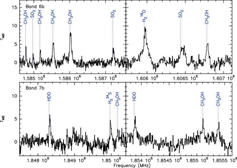
The SSB spectra for Bands 6b and 7b are given in Fig. 1 smoothed to a velocity resolution of 4.5 km s-1 and corrected for a VLSR = 9 km s-1 with the most prominent lines (peak TMB 7 K) labelled. Polynomial baselines of order 2 are also subtracted from each spectrum. We find that these observations are dominated by strong lines of CO, H2O, and OH as was reported by Lerate et al. (2006). With the higher spectral resolution of HIFI, we also detect additional strong lines of CH3OH, H2S, HCN, and HDO. Line identifications were made with the aid of the XCLASS program111http://www.astro.uni-koeln.de/projects/schilke/XCLASS which accesses both the CDMS (Müller et al., 2001, 2005, http://www.cdms.de) and JPL (Pickett et al., 1998, http://spec.jpl.nasa.gov) molecular databases. We list these transitions along with their integrated intensities in Table 2. Line intensities were measured using the CLASS data reduction and analysis software package. In instances where there were blends, Gaussian profiles were fit to the lines and the results from the fitted profiles are reported; otherwise the total intensity is measured directly using the BASE command. All line intensities were measured using spectra smoothed to a velocity resolution of 1 km s-1. Uncertainties in the integrated intensities, , were computed using the relation (K km s-1) = where is the resolution in velocity space, N is the number of channels over which the intensity is measured, and RMS is the root mean square deviation in the vicinity of the line. In addition to the lines listed in Table 2, we also detect many additional weak transitions of CH3OH, SO2, H2S, and H2O along with their isotopologues. Examples of several weak lines detected in Bands 6b and 7b are plotted in Fig. 2. Integrated line intensities for these weaker transitions along with peak intensities for all lines will be reported in a later study.
When comparing these spectra to other lower frequency HIFI bands, it is readily apparent that the line density is significantly diminished when compared to the lower frequency bands (see e.g. Bergin et al., 2010, this volume; Wang et al., 2010, in press). We estimate that the total fraction of channels taken up by lines is 0.23 in the lower frequency bands compared to 0.07 in Bands 6 and 7. We reached these estimates by counting the number of channels in emission in the frequency ranges 858.1 – 958.1 GHz (Band 3b) and 1788.4 – 1898.5 GHz (Band 7b). We adopt these line density estimates as being representative of the low and high frequency bands, respectively. Although not formally presented in this Letter, a full spectral scan of Orion KL taken in Band 3b was also obtained as part of the HEXOS key program and used to estimate the line density here. These data were reduced in the same way as Bands 6b/7b. Both bands were smoothed to a velocity resolution of 1 km s-1 and any channel that had a value TMB 2.5 K (after baseline subtraction) was flagged as being in emission in 7b. This threshold is approximately what we have estimated as 3 the RMS in TMB in Band 7b at a resolution of 1 km s-1 (RMS 0.8 K). Because the beam size, , decreases as a function of frequency (24′′), this value was scaled to an equivalent RMS in Band 3b using the following relation,
| (1) |
which assumes that the source is significantly smaller than both beam sizes. Thus the reduced beam size should be more coupled to the smaller spatial components (e.g. the hot core). One might therefore naively expect the line density to increase at THz frequencies. The opposite trend, however, is observed.
| Molecule | Frequency | Transition | Notes | |
| (MHz) | (K km s-1) | |||
| Band 6b | ||||
| H2O | 1574232.073 | 64,3 – 71,6 | 70.8 6.7 | |
| CH3OH | 1586012.991 | 85,1 – 74,1 | 85.3 3.0 | 3 |
| 1586013.008 | 85,0 – 74,0 | 3 | ||
| H2S | 1592669.425 | 72,5 – 71,6 | 69.5 3.4 | |
| HCN | 1593341.504 | 18–17 | 138.4 5.5 | 1 |
| H234S | 1595984.323 | 42,3 – 31,2 | 76.3 5.1 | |
| CH3OH | 1597947.024 | 96,0 – 85,0 | 84.4 4.1 | 3 |
| 1597947.024 | 96,1 – 85,1 | 3 | ||
| H2S | 1599752.748 | 42,3 – 31,2 | 258.0 6.4 | |
| H2O | 1602219.182 | 41,3 – 40,4 | 959.0 8.5 | |
| H234S | 1605957.883 | 61,5 – 60,6 | 116.0 6.0 | 3 |
| H218O | 1605962.460 | 41,3 – 40,4 | 3 | |
| H2S | 1608602.794 | 62,5 – 61,6 | 91.8 4.2 | |
| CO | 1611793.518 | 14 – 13 | 4653.0 12.0 | 2 |
| H218O | 1633483.600 | 22,1 – 21,2 | 192.0 9.3 | 3 |
| CH3OH | 1633493.496 | 134,0 – 123,0 | 3 | |
| H2S | 1648712.816 | 42,2 – 33,1 | 124.9 4.9 | 1 |
| 13CO | 1650767.302 | 15 – 14 | 287.0 8.0 | 3 |
| CH3OH | 1650817.827 | 214,0 – 203,0 | 3 | |
| H218O | 1655867.627 | 21,2 – 10,1 | 75.6 8.2 | 2 |
| H2O | 1661007.637 | 22,1 – 21,2 | 1008.0 9.2 | 2 |
| H217O | 1662464.387 | 21,2 – 10,1 | 155.0 7.4 | 2 |
| H2O | 1669904.775 | 21,2 – 10,1 | 2266.0 10.4 | 2 |
| HCN | 1681615.473 | 19 – 18 | 136.0 5.8 | |
| CH3OH | 1682556.723 | 105,1 – 94,1 | 76.6 3.9 | 3 |
| 1682556.856 | 105,0 – 94,0 | 3 | ||
| HDO | 1684605.824 | 61,5 – 60,6 | 71.9 4.2 | |
| Band 7b | ||||
| H2O | 1794788.953 | 62,4 – 61,5 | 969.0 8.5 | |
| H2O | 1797158.762 | 73,4 – 72,5 | 648.0 4.9 | |
| NH3 | 1808935.550 | 31,1 – 21,0 | 158.0 6.4 | 2 |
| NH3 | 1810377.792 | 32,1 – 22,0 | 50.1 8.3 | 2 |
| H218O | 1815853.411 | 53,2 – 52,3 | 91.0 5.5 | |
| CH3OH | 1817752.285 | 77,0 – 66,0 | 35.7 3.2 | |
| OH | 1834747.350 | – 1/2+ | 627.0 9.7 | 2, 4 |
| OH | 1837816.820 | – 1/2- | 640.0 11.5 | 2, 4 |
| CO | 1841345.506 | 16 – 15 | 3820.0 10.4 | 2 |
| H2S | 1846768.559 | 61,6 – 50,5 | 237.0 5.8 | |
| H2S | 1852685.693 | 51,4 – 42,3 | 181.0 4.8 | |
| H2S | 1862435.697 | 52,4 – 41,3 | 84.7 5.2 | |
| H2S | 1865620.670 | 33,0 – 22,1 | 173.6 7.8 | |
| H2O | 1867748.594 | 53,2 – 52,3 | 864.0 8.8 | |
| H2O | 1880752.750 | 63,4 – 70,7 | 135.0 5.4 | |
| H2S | 1882773.396 | 83,6 – 82,7 | 37.9 4.0 | |
| H2O | 1893686.801 | 33,1 – 40,4 | 265.0 5.9 | |
| H218O | 1894323.823 | 32,2 – 31,3 | 161.0 6.4 | |
| H2S | 1900140.572 | 71,6 – 70,7 | 83.80 6.7 | 3 |
| 1900177.906 | 72,6 – 71,7 | 3 |
4 Discussion
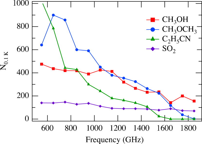
One of the primary reasons for the reduced line density in the high frequency bands is the fall off in emission from complex organic molecules – in particular the “weeds” such as CH3OCH3, SO2, C2H5CN, and, of course, CH3OH. In Fig. 3 we present the number of emissive lines for select “weeds” as a function of frequency. To estimate these numbers we assumed LTE and predicted the emission for each species assuming T K. We use the total column estimated for each molecule on the basis of Comito et al. (2005) and in addition assumed a velocity width of 5 km s-1. If the predicted emission was above 0.1 K then we counted the line as potentially emissive in our 100 GHz bins. In this fashion we counted , which is shown in the figure. As can be seen, there is a general decrease in emission for all species but its particularly evident for CH3OCH3 and C2H5CN. CH3OH has a small factor of 2 decrease in the number of lines and, at the zeroth level, this is seen in our data which has numerous weak methanol transitions scattered throughout the band.
Another possibility is that the dust emission from the hot core is optically thick in the high frequency bands; thus the dust would absorb all of the photons emitted from the molecules in the hot core. To explore this more closely we can examine the dust opacity expected within the hot core itself. Plume et al. (2010, in preparation) used multiple transitions of C18O and spectrally isolated the hot core. They estimate an N(C18O) = 1.71016 cm-2 which yields a total H2 column of 3.41023 cm-2 assuming n(C18O)/n(H2) = 1.710-7 (Frerking et al., 1982). Using the relation given in Hildebrand (1983, Equation 10), we estimate a 0.1 at 171 m, putting it slightly lower than being optically thick.
It is clear that there are other emission components in this region as we see widespread emission from a variety of molecules in the high frequency bands. However, we still observe many molecules (CH3OH, H2O, HDO, and HCN) that have velocity components in their spectral profiles that are coincident to those expected from the hot core and other components (e.g. the outflows). If these emission components do arise in the the hot core, it is likely that the molecular emission region must lie in front of any optically thick core. Given the presence of strong physical gradients in the density and temperature profiles (Wright et al., 1996; Blake et al., 1996) and the fact that the dust is marginally optically thick, this is not unrealistic.
A final contributor to the decrease in the line emission could be non-LTE excitation. At high frequencies there are a larger number of high excitation lines which could be more difficult to excite even at densities of 106 – 107 cm-3. This needs to be more directly calculated using a molecule such as CH3OH with collision rates that extend to temperatures greater than 200 – 300 K.
5 Summary
We have characterized the high frequency spectrum of Orion KL. We find that the spectrum is dominated by strong lines of CO, H2O, HDO, OH, CH3OH, H2S, HCN, and NH3. We also detect many weaker transitions of CH3OH, H2O, HDO, and SO2. We find that the line density is diminished in the high frequency bands when compared to the lower frequency bands and provide a number of explanations as to why this may be.
Acknowledgements.
HIFI has been designed and built by a consortium of institutes and university departments from across Europe, Canada and the United States under the leadership of SRON Netherlands Institute for Space Research, Groningen, The Netherlands and with major contributions from Germany, France and the US. Consortium members are: Canada: CSA, U.Waterloo; France: CESR, LAB, LERMA, IRAM; Germany: KOSMA, MPIfR, MPS; Ireland, NUI Maynooth; Italy: ASI, IFSI-INAF, Osservatorio Astrofisico di Arcetri- INAF; Netherlands: SRON, TUD; Poland: CAMK, CBK; Spain: Observatorio Astron mico Nacional (IGN), Centro de Astrobiolog a (CSIC-INTA). Sweden: Chalmers University of Technology - MC2, RSS & GARD; Onsala Space Observatory; Swedish National Space Board, Stockholm University - Stockholm Observatory; Switzerland: ETH Zurich, FHNW; USA: Caltech, JPL, NHSC. Support for this work was provided by NASA through an award issued by JPL/Caltech. CSO is supported by the NSF, award AST-0540882.References
- Bergin et al. (2010, this volume) Bergin, E. A., Phillips, T. G., Comito, C., et al. 2010, A&A, this volume
- Blake et al. (1996) Blake, G. A., Mundy, L. G., Carlstrom, J. E., et al. 1996, ApJ, 472, L49+
- Blake et al. (1987) Blake, G. A., Sutton, E. C., Masson, C. R., & Phillips, T. G. 1987, ApJ, 315, 621
- Comito et al. (2005) Comito, C., Schilke, P., Phillips, T. G., et al. 2005, ApJS, 156, 127
- de Graauw et al. (2010) de Graauw, T., Helmich, F. P., Phillips, T. G., et al. 2010, A&A, 518, L6+
- Frerking et al. (1982) Frerking, M. A., Langer, W. D., & Wilson, R. W. 1982, ApJ, 262, 590
- Hildebrand (1983) Hildebrand, R. H. 1983, QJRAS, 24, 267
- Kleinmann & Low (1967) Kleinmann, D. E. & Low, F. J. 1967, ApJ, 149, L1+
- Lerate et al. (2006) Lerate, M. R., Barlow, M. J., Swinyard, B. M., et al. 2006, MNRAS, 370, 597
- Menten et al. (2007) Menten, K. M., Reid, M. J., Forbrich, J., & Brunthaler, A. 2007, A&A, 474, 515
- Müller et al. (2005) Müller, H. S. P., Schlöder, F., Stutzki, J., & Winnewisser, G. 2005, Journal of Molecular Structure, 742, 215
- Müller et al. (2001) Müller, H. S. P., Thorwirth, S., Roth, D. A., & Winnewisser, G. 2001, A&A, 370, L49
- Ott (2010) Ott, S. 2010, in ASP Conference Series, Astronomical Data Analysis Software and Systems XIX,Y. Mizumoto, K. I. Morita, and M.Ohishi, eds., in press
- Persson et al. (2007) Persson, C. M., Olofsson, A. O. H., Koning, N., et al. 2007, A&A, 476, 807
- Pickett et al. (1998) Pickett, H. M., Poynter, I. R. L., Cohen, E. A., et al. 1998, Journal of Quantitative Spectroscopy and Radiative Transfer, 60, 883
- Pilbratt et al. (2010) Pilbratt, G. L., Riedinger, J. R., Passvogel, T., et al. 2010, A&A, 518, L1+
- Schilke et al. (1997) Schilke, P., Groesbeck, T. D., Blake, G. A., & Phillips, T. G. 1997, ApJS, 108, 301
- Tercero et al. (2010) Tercero, B., Cernicharo, J., Pardo, J. R., & Goicoechea, J. R. 2010, ArXiv e-prints
- Wang et al. (2010, in press) Wang, S., Bergin, E. A., Crockett, N. R., et al. 2010, A&A, in press
- Wright et al. (1996) Wright, M. C. H., Plambeck, R. L., & Wilner, D. J. 1996, ApJ, 469, 216