Hydrodynamic Correlation Functions of a Driven Granular Fluid in Steady State

Abstract

We study a homogeneously driven granular fluid of hard spheres at intermediate volume fractions and focus on time-delayed correlation functions in the stationary state. Inelastic collisions are modeled by incomplete normal restitution, allowing for efficient simulations with an event-driven algorithm. The incoherent scattering function, $F_{\rm incoh}(q,t)$, is seen to follow time-density superposition with a relaxation time that increases significantly as volume fraction increases. The statistics of particle displacements is approximately Gaussian. For the coherent scattering function $S(q,\omega)$ we compare our results to the predictions of generalized fluctuating hydrodynamics which takes into account that temperature fluctuations decay either diffusively or with a finite relaxation rate, depending on wave number and inelasticity. For sufficiently small wave number $q$ we observe sound waves in the coherent scattering function $S(q,\omega)$ and the longitudinal current correlation function $C_{\mathrm{l}}(q,\omega)$. We determine the speed of sound and the transport coefficients and compare them to the results of kinetic theory.

I I Introduction

The long wavelength, low frequency dynamics of granular fluids is frequently described by phenomenological hydrodynamic equations Campbell (1990); Brey et al. (1998); Sela and Goldhirsch (1998); Goldhirsch (2003). In contrast to a fluid composed of elastically colliding particles, the total energy of the system is not conserved, implying a finite decay rate of the temperature in the limit of long wavelength. Hence, strictly speaking, the temperature is not a hydrodynamic variable. More generally, the scale separation required by hydrodynamics has been questioned Tan and Goldhirsch (1998). If the system is not driven, the homogeneous state is unstable Goldhirsch and Zanetti (1993) and large spatial gradients develop — invalidating a hydrodynamic approach. A third point of criticism refers to the pressure in the Navier-Stokes equation. Closure of the hydrodynamic equations requires an equation of state to express the pressure Herbst et al. (2004) in terms of density and temperature. However, an equation of state is expected to exist only in an equilibrium state. Given these problems, the hydrodynamic approach has been mainly restricted to small inelasticity, such that the decay rate of the temperature is small, the time for the build-up of spatial inhomogeneities is long, and an equation of state is approximately valid. In this limit, kinetic theory has provided a basis for the hydrodynamic equations and given explicit expressions for the transport coefficients Jenkins and Savage (1983); Lun et al. (1984); Brilliantov and Pöschel (2004).

Driving a granular fluid allows for a compensation of the energy which is dissipated in collisions, such that a non-equilibrium stationary state (NESS) is reached. In experiment, the driving is frequently performed by shearing Lutsko (2001); Santos (2008), with vibrating walls Olafsen and Urbach (1999); Reyes and Urbach (2008); Brey and Ruiz-Montero (2010) or by driving the system homogeneously Schröter et al. (2005); Abate and Durian (2006). To test a hydrodynamic approach in the NESS we want to avoid new length scales, which might be generated by driving through the boundaries, when the agitation decays over a characteristic length, e.g. the width of a shear band. Hence in the following, we consider a homogeneously driven granular fluid van Noije et al. (1998, 1999); Pagonabarraga et al. (2001); Fiege et al. (2009); Kranz et al. (2010) and set out to investigate the validity of the hydrodynamic approach in the NESS.

We present in this paper results for a homogeneously driven system of hard spheres with moderate inelasticity, parametrized by a coefficient of restitution $\epsilon=0.8,0.9$ and $1.0$ (elastic). We use event-driven simulations to focus on the dynamics of the system. Previous studies of correlation functions for granular fluids have been either on density-density correlations at the same time, such as the structure factor $S(q)$ van Noije et al. (1998, 1999) and the pair correlation function Panaitescu and Kudrolli (2010), or on velocity-velocity correlations Fiege et al. (2009) (and references therein). We focus here on time dependent spatial correlations Kranz et al. (2010) at volume fraction $0.05\leq\eta\leq 0.4$ and compute the incoherent and coherent intermediate scattering functions.

The former entails information about the motion of a tagged particle, which is expected to be diffusive at long times. We find that the incoherent scattering function is well approximated by a Gaussian and obeys time-density superposition. The divergence of the relaxation time as a function of $\eta$ occurs not only for the elastic case but also for the inelastic case, consistent with the results of Reyes et al. Reyes and Urbach (2008) and Kranz et al. (2010).

The coherent correlations reveal the collective dynamics of the fluid: damped sound waves and relaxation of temperature fluctuations. We determine the dynamic structure factor $S(q,\omega)$ and compare our data quantitatively to the predictions of van Noije et al. van Noije et al. (1999) using fluctuating hydrodynamics. The agreement between simulations and theory is quite good: damped sound waves are indeed observed for small wave numbers $q$ and the velocity and damping of sound can be determined. Temperature fluctuations are found to decay either diffusively or with a finite rate, depending on $q$. The transport coefficients are compared to the predictions of kinetic theory and found to agree well.

In the following we specify model and simulation details in Sec. II. Subsequently, in Sec. III we discuss the incoherent scattering function, the mean square displacement, and the diffusion constant. Data for the intermediate coherent scattering function and longitudinal current correlation function are presented in Sec. IV. A hydrodynamic model, which was first introduced in Ref. van Noije et al. (1998), is discussed in Sec. V and compared to the simulation data for the coherent scattering function in Sec. VI.

II II Model and Simulation Details

We investigate a system of $N$ monodisperse hard spheres of diameter $a$ and mass $m$ at volume fraction $\eta=\frac{N\pi a^{3}}{6V}$. The time evolution is governed by instantaneous inelastic two-particle collisions. We consider here only the simplest model of an inelastic two-body collision, described by incomplete normal restitution. The change of the relative velocity $\mathbf{g}:=\mathbf{v}_{1}-\mathbf{v}_{2}$ of the two colliding particles is given by

$$\left(\mathbf{g}\cdot\mathbf{n}\right)^{\prime}=-\varepsilon\left(\mathbf{g}\cdot\mathbf{n}\right),$$ (1)

where primed quantities indicate post-collisional velocities and unprimed ones refer to precollisional ones. The unit vector $\mathbf{n}:=(\mathbf{r}_{1}-\mathbf{r}_{2})/\left|(\mathbf{r}_{1}-\mathbf{r}_{2})\right|$ connects the centers of the two spheres, and $\varepsilon=$const. $\in\left[0,1\right]$ denotes the coefficient of normal restitution, with $\varepsilon=1.0$ in the elastic limit. The postcollisional velocities of the two colliding spheres are given by

$${\mathbf{v}}_{1}^{\prime}=\mathbf{v}_{1}-\frac{\left(1+\varepsilon\right)}{2}(\mathbf{n}\cdot\mathbf{g})\mathbf{n}$$ (2)

$${\mathbf{v}}_{2}^{\prime}=\mathbf{v}_{2}+\frac{\left(1+\varepsilon\right)}{2}(\mathbf{n}\cdot\mathbf{g})\mathbf{n}.$$ (3)

Due to the inelastic nature of the collisions, we have to feed energy into the system in order to maintain a stationary state. The simplest bulk driving Williams and MacKintosh (1996) consists of a kick of a given particle, say particle $i$, instantaneously at time $t$, which corresponds to

$$\mathbf{v}_{i}(t)=\mathbf{v}_{i}(t_{o})+\int_{t_{0}}^{t}ds\bm{\xi}_{i}(s).$$ (4)

The noise $\bm{\xi}_{i}(t)$ is Gaussian with zero mean and variance

$$\langle\xi_{i}^{(\alpha)}(t)\xi_{j}^{(\beta)}(t^{\prime})\rangle=\xi_{0}^{2}\delta_{i,j}\delta_{\alpha\beta}\delta(t-t^{\prime})$$ (5)

for the cartesian components $\xi_{i}^{(\alpha)}$, $\alpha=x,y,z$. The stochastic process is implemented in the simulation by kicking the particles randomly with amplitude $v_{\mathrm{Dr}}$ and frequency $f_{\mathrm{Dr}}$.

If a single particle is kicked at a particular instant, momentum is not conserved. Due to the random direction of the kicks the time average will restore the conservation of global momentum, but only on average. Momentum conservation is known to be essential for the dynamic correlation functions in the limit of long wavelength and long times. Hence we choose a driving mechanism in which pairs of particles are kicked in opposite directions Espanol and Warren (1995). The pairs are fixed globally so that the total momentum is conserved at each instant of time. Denoting the partner of particle $i$ by $p(i)$, the random force correlation is given by

$$\langle\xi_{i}^{(\alpha)}(t)\xi_{j}^{(\beta)}(t^{\prime})\rangle=\xi_{0}^{2}(\delta_{j,i}-\delta_{j,p(i)})\delta_{\alpha\beta}\delta(t-t^{\prime}).$$ (6)

It is also possible to ensure momentum conservation on small scales by choosing pairs of neighboring particles and by kicking them in opposite directions. However this is not pursued here.

For the event-driven simulations we use the optimized algorithm of Lubachevsky Lubachevsky (1991) adapted to granular media Fiege et al. (2009). To avoid the inelastic collapse we use the technique of virtual hulls around the spheres as described in Fiege et al. (2009). Particles are colliding elastically when they are a diameter $a$ apart and the dissipation takes place when the colliding spheres are receding and separated by $\left(1+10^{-4}\right)a$. With the appropriate choice of $v_{\mathrm{Dr}}^{2}f_{\mathrm{Dr}}=\xi_{0}^{2}$ we ensured constant temperature and in all following we chose units such that $m=a=T=1$. All simulations were with a cubic box and periodic boundary conditions. The simulation results of Sec. III are for $N=200000$ and two independent simulation runs , whereas for the results of Sec. IV and Sec. VI we needed more statistics and therefore used $N=10000$ and 100 independent simulation runs. In each set of simulations we first equilibrated at $\varepsilon=1.0$ at the desired volume fraction, followed by a relaxation to a stationary state at $\varepsilon\neq 1$ (achieved with a simulation run of at least 100 time units) and consecutive production runs. Independent configurations were taken from the initial elastic equilibration run separated in time by at least 1000 time units.

III III Intermediate Incoherent Scattering Function and Self Diffusion Constant

In this section we investigate time delayed correlations of a single tagged particle. In Fig. 1 we show for volume fractions $0.05\leq\eta\leq 0.4$ and for inelasticities $\varepsilon=0.8,0.9,1.0$ the incoherent intermediate scattering function

$$F_{\mathrm{incoh}}(\mathbf{q},t)=\left\langle\frac{1}{N}\sum_{i=1}^{N}e^{i\mathbf{q}\cdot(\mathbf{r}_{i}(t)-\mathbf{r}_{i}(0)}\right\rangle.$$ (7)

Since $F_{\mathrm{incoh}}(\mathbf{q},t)$ is a measure of the correlation of particle $i$ at position $\mathbf{r}_{i}(t)$ at time $t$ and at position $\mathbf{r}_{i}(0)$ at time $t=0$, we find as expected that $F_{\mathrm{incoh}}(\mathbf{q},t)$ decreases with increasing time. With decreasing densities the $\mathbf{r}_{i}(t)$ and $\mathbf{r}_{i}(0)$ become more quickly uncorrelated and therefore the decay is faster for smaller volume fractions. For the lowest densities the inelastic system can hardly be distinguished from the elastic case. For higher densities the relaxation is increasingly faster for the more inelastic systems. To quantify this effect we plot in Fig. 2 the relaxation time $\tau$ when the incoherent intermediate scattering function has decayed to $1/e$ of its initial value, i.e. $F_{\mathrm{incoh}}(\mathbf{q},\tau)=1/e$. Clearly the elastic system shows the most rapid increase of relaxation time with density, even though the highest volume fraction ($\eta=0.4$) is still well below the critical value for the glass transition. The slowing down is weaker for the inelastic systems. However, the inelastic system also shows an increase by a factor of 12 ($\varepsilon=0.9$) and 7 ($\varepsilon=0.8$). This indication for a precursor of a glass transition even for the inelastic system is consistent with the higher density results of Kranz et al. Kranz et al. (2010) (theory and simulation) and of Reis et al. Reis et al. (2007) and Reyes et al. Reyes and Urbach (2008) (experiment.)

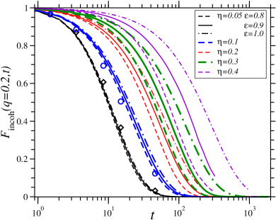
Figure 1: Incoherent intermediate scattering function for several values of volume fraction $\eta$ and coefficient of restitution $\varepsilon$. All lines for $N=200000$ where $\varepsilon=0.8/0.9/1.0$ are indicated with dashed/solid/dot-dashed lines respectively. $\eta=0.05$ corresponds to the left and $\eta=0.4$ to the right lines. All error bars are of the order of $10^{-3}$. Open diamonds and circles are for $N=10000$, $\varepsilon=0.8$ and $\eta=0.05,0.1$ respectively.

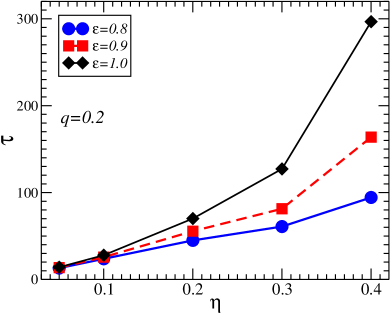
Figure 2: Relaxation time of the incoherent scattering function as a function of volume fraction $\eta$ for several values of $\varepsilon$ for simulation runs with $N=200000$ particles.

The intermediate incoherent scattering function, $F_{\mathrm{incoh}}(\mathbf{q},t)$, is often approximated by a Gaussian

$$F_{\mathrm{incoh}}(\mathbf{q},t)=e^{\frac{-q^{2}}{6}\left\langle\Delta r^{2}(t)\right\rangle},$$ (8)

assuming that the mean square displacement

$$\left\langle\Delta r^{2}(t)\right\rangle=\left\langle\frac{1}{N}\sum_{i=1}^{N}\big{(}\mathbf{r}_{i}(t)-\mathbf{r}_{i}(0)\big{)}^{2}\right\rangle$$ (9)

obeys Gaussian statistics. To test this hypothesis we first compute the mean square displacement $\left\langle\Delta r^{2}(t)\right\rangle$. Fig. 3 shows the resulting $\left\langle\Delta r^{2}(t)\right\rangle$ for $\varepsilon=0.8$ and several volume fractions. One clearly observes a ballistic regime for small times with a crossover to diffusive behavior around $t\sim 1$.

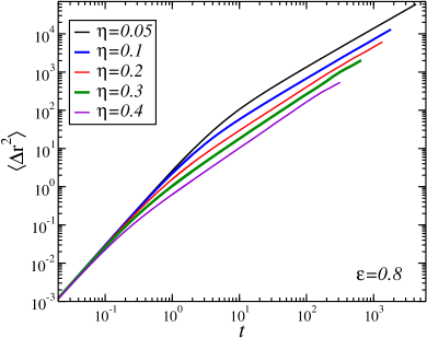
Figure 3: Mean square displacement for $\varepsilon=0.8$ and various volume fractions.

The computed $\left\langle\Delta r^{2}(t)\right\rangle$ is then substituted in the Gaussian approximation of Eq. (8) and compared to the full scattering function in Fig. 4. The Gaussian approximation works very well for the densities under consideration, in particular for small $q$.

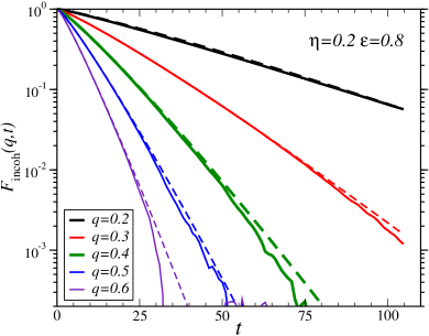
Figure 4: Intermediate incoherent scattering function $F_{\mathrm{incoh}}(\mathbf{q},t)$ using Eq. (7) (solid lines) and for comparison the Gaussian approximation using Eqs. (8) and (9) (dashed lines.)

We can also extract the self diffusion,

$$D=\lim_{t\to\infty}\frac{\left\langle\Delta r^{2}(t)\right\rangle}{6t},$$ (10)

via a linear fit to $\left\langle\Delta r^{2}(t)\right\rangle$ at long times. The resulting $D$ is plotted in Fig. 5 as a function of density (filled symbols) and compared with theoretical predictions (open symbols). As expected, the diffusion constant decreases strongly with density. Whereas the prediction of Enskog (see Eq. (5) of Fiege et al. (2009)) is in excellent agreement for the elastic case (see inset), the prediction of Garzó Garzó et al. (2007) is very good for the inelastic case and $\eta>0.1$.

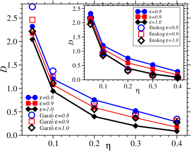
Figure 5: Self diffusion constant $D$ as a function of volume fraction $\eta$. The filled symbols with lines for the eye are obtained via linear fits to the mean-square displacement for large times. Garzó results are corresponding to Eq. (2.10) of Garzó et al. (2007) and the Enskog result corresponds to Eq. (5) of Fiege et al. (2009).

For the glass transition in elastic systems, one observes dynamic scaling as the transition is approached. In other words, the scattering function does not depend separately on time and control parameter — either temperature or density — but only on the ratio $t/\tau$. We have tested this time-density superposition principle by plotting $F_{\mathrm{incoh}}(\mathbf{q},t/\tau)$ for five volume fractions in Fig. 6. Even though the volume fractions under consideration are far away from the critical value, the data collapse for $\eta\geq 0.1$.

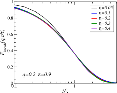
Figure 6: Time-density superposition for the incoherent scattering function.

IV IV Intermediate Coherent Scattering Function and Longitudinal Current Correlation

Information about the collective dynamics and in particular collective density fluctuations is contained in the intermediate coherent scattering function, defined by

$$F(\mathbf{q},t)=\left\langle\frac{1}{N}\sum_{i,j=1}^{N}e^{i\mathbf{q}\cdot(\mathbf{r}_{i}(t)-\mathbf{r}_{j}(0)}\right\rangle.$$ (11)

In the hydrodynamic regime, i.e. small wave numbers, we expect to see sound modes. This expectation is indeed born out by the data with an example shown in Fig. 7 for volume fraction $\eta=0.1$, restitution coefficient $\epsilon=0.9$, and for several $q$ values. We observe oscillations which are overdamped for large $q$.

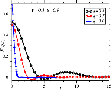
Figure 7: Intermediate coherent scattering function $F(q,t)$.

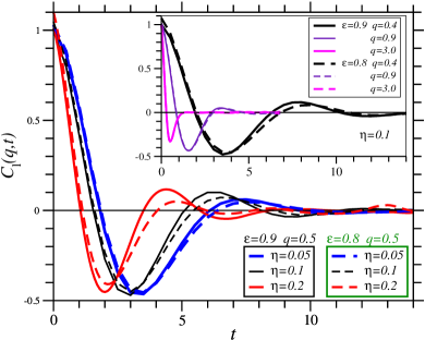
Figure 8: Longitudinal current correlation as a function of time for several densities; inset: variation with $q$.

A detailed analysis of the coherent correlation in terms of damped sound waves and temperature fluctuations will be given in Sec. VI, using a hydrodynamic model discussed in the next section. Here we consider the longitudinal current correlation to obtain an approximation to the sound velocity which we analyze in dependence on volume fraction and inelasticity. The correlation of the longitudinal current is defined as

$$C_{l}(\mathbf{q},t) = \left\langle\frac{1}{N}\sum_{i,j=1}^{N}\frac{1}{q^{2}}\left(\mathbf{q}\cdot\mathbf{v}_{i}\right)\,\left(\mathbf{q}\cdot\mathbf{v}_{j}\right)e^{i\mathbf{q}\cdot(\mathbf{r}_{i}(t)-\mathbf{r}_{j}(0)}\right\rangle$$ (12)

$$= -\frac{1}{q^{2}}\partial_{t}^{2}F(\mathbf{q},t).$$

In Fig. 8 we show data for two values of restitution and volume fractions $0.05\leq\eta\leq 0.2$. For all parameters we observe well-defined oscillations which are more strongly damped for the more inelastic system.

In Fig. 9 we plot $C_{l}(\mathbf{q},\omega)$ the corresponding Fourier transform of the current correlation.

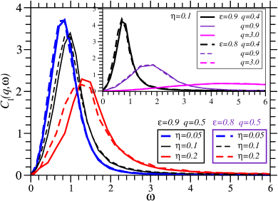
Figure 9: Longitudinal current correlation as a function of angular frequency.

The position of the maximum of $C_{l}(\mathbf{q},\omega)$ can be used to estimate the speed of sound. The peak position $\omega_{\mathrm{max}}$ as a function of wave number $q$ is shown in Fig. 10. As shown in the inset, the peak position does not depend on $\varepsilon$. For small wave numbers a linear dispersion is observed (dashed lines in Fig. 10), while deviations from linear behavior for larger wave numbers are more pronounced for the denser systems.

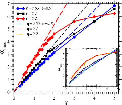
Figure 10: Position of the maximum, $\omega_{\mathrm{max}}$ of longitudinal current correlation $C_{l}(\mathbf{q},\omega)$. Solid lines and filled symbols are for $\epsilon=0.9$ and dashed lines indicate linear fits with slopes as listed in Table 3. The inset shows for comparison $\omega_{\mathrm{max}}$ for $\epsilon=0.9$ (solid lines) and for $\epsilon=0.8$ (dash-dotted lines).

V V Fluctuating Hydrodynamics

In this section we compute $S(q,\omega)$ from fluctuating hydrodynamics. Our presentation follows closely the work of van Noije et al. van Noije et al. (1999), except that we take care to conserve momentum at each instant of time, thereby avoiding a divergence of the static structure factor.

The hydrodynamic equations for the number density $n$ and flow velocity $\mathbf{u}$ are the same as for an elastic fluid. However the equation for the temperature differs due to the energy dissipation in collisions and the energy input due to driving:

$$\partial_{t}T=D_{T}\Delta T-\frac{2p}{dn}\nabla\mathbf{u}-\Gamma+m\xi_{0}^{2}+\theta.$$ (13)

Here we present results in $d=3$ dimensions. The energy dissipation due to collisions, $\Gamma$, is estimated as $\Gamma=2T\nu_{\mathrm{coll}}\frac{1-\varepsilon^{2}}{2d}$ with the collision frequency $\nu_{\mathrm{coll}}$. The input of kinetic energy due to driving is given by $m\xi_{0}^{2}$, $p$ denotes the pressure and $D_{T}$ the thermal diffusivity. We have ignored nonlinear terms involving the flow field because we will consider only linear hydrodynamics. In the stationary state the energy dissipation in collisions and the energy input due to driving balance on average:

$$\Gamma_{0}=m\xi_{0}^{2}.$$ (14)

We expand in fluctuations around the stationary state: $n=n_{0}+\delta n,T=T_{0}+\delta T$ and $\Gamma=\Gamma_{0}+\delta\Gamma$. The collision frequency should be proportional to the density, the pair correlation function at contact, $\chi$, and the thermal velocity: $\nu_{\mathrm{coll}}\propto n\chi T^{1/2}$, hence linearization around the stationary state $\Gamma_{0}$ yields: $\Gamma\sim\Gamma_{0}(1+\frac{\delta n}{n_{0}}+\frac{1}{\chi}\frac{\mathrm{d}\chi}{\mathrm{d}n}\delta n+\frac{3\delta T}{2T_{0}})$.

Following van Noije et al. van Noije et al. (1999), we consider a hydrodynamic description of a granular fluid based on conservation of particle number and momentum and the relaxation of temperature to its stationary value, $T_{0}$. The transverse momentum decouples so that we are left with three equations for the fluctuating density $\delta n$, the longitudinal flow velocity $u(\mathbf{q},t)=\mathbf{q}\cdot\mathbf{u}/q$, and the fluctuating temperature $\delta T$:

$$\partial_{t}\delta n(\mathbf{q},t) = -iqn_{0}u(\mathbf{q},t)$$ (15)

$$\partial_{t}u(\mathbf{q},t) = -\frac{iq}{mn_{0}}\left(\frac{\partial p}{\partial n}\delta n(\mathbf{q},t)+\frac{\partial p}{\partial T}\delta T(\mathbf{q},t)\right)$$

$$- \nu_{\mathrm{l}}q^{2}u(\mathbf{q},t)+\xi_{\mathrm{l}}(\mathbf{q},t)$$

$$\partial_{t}\delta T(\mathbf{q},t) = -D_{T}q^{2}\delta T(\mathbf{q},t)-iq\frac{2p_{0}}{dn_{0}}u(\mathbf{q},t)$$

$$- \Gamma_{0}\left(\frac{\delta n(\mathbf{q},t)}{n_{0}}+\frac{1}{\chi}\frac{\mathrm{d}\chi}{\mathrm{d}n}\delta n(\mathbf{q},t)+\frac{3}{2}\frac{\delta T(\mathbf{q},t)}{T_{0}}\right)$$

$$+ \theta(\mathbf{q},t),$$

where $D_{T}=\frac{2\kappa}{dn_{0}}$ with the heat conductivity $\kappa$, and where $\nu_{\mathrm{l}}$ is the longitudinal viscosity. Fluctuating hydrodynamics for an elastic fluid ($\epsilon=1$) is based on internal noise, $\xi^{\mathrm{in}}_{\mathrm{l}}$ and $\theta^{\mathrm{in}}$, consistent with the fluctuations-dissipation theorem. Here we consider a randomly driven system: the particles are kicked randomly, giving rise to external noise in the equation for the velocity as well as the temperature. The external contributions are

$$\xi_{\mathrm{l}}^{\mathrm{ex}}(\mathbf{r},t)=\frac{1}{n_{0}}\sum_{i}\xi_{i\mathrm{l}}(t)\delta(\mathbf{r}-\mathbf{r}_{i})$$ (18)

and

$$\theta^{\mathrm{ex}}(\mathbf{r},t)=\frac{2m}{dn_{0}}\sum_{i}\mathbf{v}_{i}\cdot\bm{\xi}_{i}(t)\delta(\mathbf{r}-\mathbf{r}_{i}(t)),$$ (19)

with variance

$$\langle\xi_{\mathrm{l}}^{\mathrm{ex}}(\mathbf{q},t)\xi_{\mathrm{l}}^{\mathrm{ex}}(-\mathbf{q},t^{\prime})\rangle=V\frac{\xi_{0}^{2}}{n_{0}}\delta(t-t^{\prime})(1-\delta_{\mathbf{q},\mathbf{0}})$$ (20)

and

$$\langle\theta^{\mathrm{ex}}(\mathbf{q},t)\theta^{\mathrm{ex}}(-\mathbf{q},t^{\prime})\rangle=V\frac{4mT_{0}}{dn_{0}}\xi_{0}^{2}\delta(t-t^{\prime})(1-\delta_{\mathbf{q},\mathbf{0}}).$$ (21)

Here we have taken care of global momentum conservation, as realized by our driving mechanisms involving pairs of particles. These terms occur only for $q=0$ and ensure that the driving force vanishes at zero wave number. Including both types of noise, $\xi_{\mathrm{l}}=\xi_{\mathrm{l}}^{\mathrm{in}}+\xi_{\mathrm{l}}^{\mathrm{ex}}$ and $\theta_{\mathrm{l}}=\theta_{\mathrm{l}}^{\mathrm{in}}+\theta_{\mathrm{l}}^{\mathrm{ex}}$, as suggested by Noije et al. van Noije et al. (1999), one obtains

$$\langle\xi_{\mathrm{l}}(\mathbf{q},t)\xi_{\mathrm{l}}(-\mathbf{q},t^{\prime})\rangle=V\left(\frac{\xi_{0}^{2}}{n_{0}}+\frac{2\nu_{\mathrm{l}}T_{0}q^{2}}{mn_{0}}\right)\delta(t-t^{\prime})(1-\delta_{\mathbf{q},\mathbf{0}})$$ (22)

and

$$\langle\theta(\mathbf{q},t)\theta(-\mathbf{q},t^{\prime})\rangle=4V\left(\frac{mT_{0}\xi_{0}^{2}}{dn_{0}}+\frac{2\kappa T_{0}^{2}q^{2}}{d^{2}n_{0}^{2}}\right)\delta(t-t^{\prime})(1-\delta_{\mathbf{q},\mathbf{0}}).$$ (23)

To complement the above equations, we need an expression for the pressure $p$ in terms of the density and temperature. Since the driven granular gas is far from equilibrium, we cannot expect that a thermodynamic description including an equation of state should hold in general. Nevertheless for small to moderate inelasticities an equation of state has been found empirically (Eq. (17.29) in Brilliantov and Pöschel (2004)): $p\approxeq nT\left(1+2\eta\chi(1+\varepsilon)\right)$. We use the Carnahan-Starling approximation (for $d=3$)

$$\chi=\frac{\left(1-\eta/2\right)}{\left(1-\eta\right)^{3}}.$$ (24)

This leaves us with two unknown parameters in the hydrodynamic description, namely the longitudinal viscosity, $\nu_{\mathrm{l}}$, and the thermal diffusivity, $D_{T}$.

The linearized equations can be solved for the frequency and wave number dependent correlation functions, $S(q,\omega)$ and $C_{l}(q,\omega)=\frac{\omega^{2}}{q^{2}}S(q,\omega)$. Of particular interest is the pole structure in the complex $\omega$-plane, describing damped sound modes and the decay of temperature fluctuations. The latter can be either diffusive or with a finite relaxation rate, depending on wave number $q$. For $D_{T}q^{2}\ll\frac{3\Gamma_{0}}{2T_{0}}$, the thermal diffusivity can be ignored and we have poles at

$$\omega_{T} = \pm i\frac{3\Gamma_{0}}{2T_{0}}$$ (25)

$$\omega_{s} = \pm cq\pm i\gamma q^{2}.$$ (26)

The latter correspond to sound modes with sound velocity

$$c^{2}=v_{\mathrm{th}}^{2}-\frac{2p_{0}}{3mn_{0}}\left(1+\frac{n_{0}}{\chi}\frac{\partial\chi}{\partial n}\right)$$ (27)

where $v_{\mathrm{th}}^{2}=\frac{1}{m}\left(\frac{\partial p}{\partial n}\right)_{T}$, and damping

$$2\gamma=\nu_{\mathrm{l}}+\frac{4p_{0}T_{0}}{3\Gamma_{0}mn_{0}}\left(\frac{1}{3}\left[1+\frac{n_{0}}{\chi}\frac{\partial\chi}{\partial n}\right]+\frac{p_{0}}{dT_{0}n_{0}}\right).$$ (28)

In the opposite limit $D_{T}q^{2}\gg\frac{3\Gamma_{0}}{2T_{0}}$, we recover ordinary hydrodynamics of an elastic fluid. The sound speed is given by the adiabatic value

$$c^{2}=v_{s}^{2}=v_{\mathrm{th}}^{2}+\frac{2p_{0}^{2}}{dmT_{0}n_{0}^{2}}$$ (29)

and the temperature decay is diffusive $\omega_{T}=\pm iD_{T}q^{2}\frac{v_{\mathrm{th}}^{2}}{v_{s}^{2}}$.

In general, we expect to see a crossover, when $D_{T}q_{\mathrm{c}}^{2}=\frac{3\Gamma_{0}}{2T_{0}}$. In order to estimate $q_{\mathrm{c}}$, we use the Enskog values for the collision frequency in three dimensions and the thermal diffusivity:

$$\nu_{\mathrm{coll}} = \omega_{\mathrm{E}}=4\pi\chi n_{0}a^{2}\sqrt{\frac{T_{0}}{\pi m}}$$ (30)

$$D_{T} = \frac{75}{d(1+\varepsilon)(49-33\varepsilon)n_{0}a^{2}\chi}\sqrt{\frac{T_{0}}{\pi m}}.$$ (31)

These yield for the crossover wave number

$$q_{\mathrm{c}}^{2}a^{2}=\frac{6(1-\varepsilon^{2})(1+\varepsilon)(49-33\varepsilon)\chi^{2}36\eta^{2}}{75\pi}.$$ (32)

Numerical values of estimated $q_{\mathrm{c}}a$ for the simulated volume fractions $\eta$ and inelasticities $\epsilon$ are given in Table 1

$\eta$	$\epsilon$	$q_{\mathrm{c}}a$
0.05	0.8	0.21
0.05	0.9	0.14
0.1	0.8	0.48
0.1	0.9	0.33
0.2	0.8	1.29
0.2	0.9	0.89

Table 1: Estimates for $q_{\mathrm{c}}a$ using Eq. (32).

For the case of $D_{T}q^{2}\approx\frac{3\Gamma_{0}}{2T_{0}}$ it is necessary to use the more general solution for the dynamic structure factor

$$S(q,\omega)=n_{0}q^{2}\left(\frac{\left[\omega^{2}+\left(3\gamma_{0}\omega_{\mathrm{E}}+D_{T}q^{2}\right)^{2}\right]\left[\frac{\xi_{0}^{2}}{n_{0}}+\frac{2\nu_{\mathrm{l}}T_{0}q^{2}}{mn_{0}}\right]+q^{2}\left(\frac{p_{0}}{mn_{0}T_{0}}\right)^{2}\left[\frac{4mT_{0}\xi_{0}^{2}}{dn_{0}}+\frac{4D_{T}T_{0}^{2}q^{2}}{dn_{0}}\right]}{\left|{\mathrm{det}}M\right|^{2}}\right),$$ (33)

where we have used $\nu_{\mathrm{coll}}=\omega_{\mathrm{E}}$, the abbreviation $\gamma_{0}=\frac{1-\varepsilon^{2}}{2d}$ and where

$$\left|{\mathrm{det}}M\right|^{2} = \left[-\omega^{2}\left(3\gamma_{0}\omega_{\mathrm{E}}+D_{T}q^{2}+\nu_{\mathrm{l}}q^{2}\right)+q^{2}\left(3\gamma_{0}\omega_{\mathrm{E}}v_{\mathrm{th}}^{2}-\frac{2p_{0}\gamma_{0}\omega_{\mathrm{E}}}{mn_{0}}\left\{1+\frac{n_{0}}{\chi}\frac{\partial\chi}{\partial n}\right\}+v_{\mathrm{th}}^{2}D_{T}q^{2}\right)\right]^{2}$$ (34)

$$+ \left[\omega^{3}-\omega q^{2}\left(3\nu_{\mathrm{l}}\gamma_{0}\omega_{\mathrm{E}}+\nu_{\mathrm{l}}D_{T}q^{2}+v_{\mathrm{th}}^{2}+\frac{2p_{0}^{2}}{dmT_{0}n_{0}^{2}}\right)\right]^{2}.$$

VI VI Coherent Scattering Function and Transport Coefficients

According to the $q_{\mathrm{c}}$ estimates given in Table 1, we see that our data are neither clearly in the hydrodynamic regime nor in the inelastic regime, but in general the two relaxation terms in the equation for the temperature are comparable in magnitude. Hence, we fit the simulation results of the dynamic structure factor to the full expression for $S(q,\omega)$ as given in Eqs. (33) and (34). We allow for two fit parameters, $D_{T}$ and $\nu_{l}$, with all other parameters determined by the approximate equation of state. The best fits (solid line) are shown in Figs. 11 – 14; in comparison with the simulation data (symbols) for $S(q,\omega)$. We find excellent agreement not only for very small $q$, for which we would expect best agreement with the hydrodynamic equations, but also for $q\lesssim 1.0$. Both features, the shoulder due to the sound wave as well as the damping, are quantitatively in agreement with Eqs. (33) and (34). Similarly, we find very good agreement for the $\eta=0.1$ results.

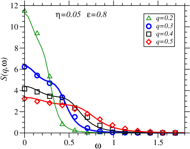
Figure 11: Dynamic structure factor $S(q,\omega)$ for $\eta=0.05,\,\varepsilon=0.8$ and $q=0.2$ – $0.5$. Symbols indicate simulation results obtained via Fourier transform of $F(q,t)$ and lines indicate fits with Eq. (33).

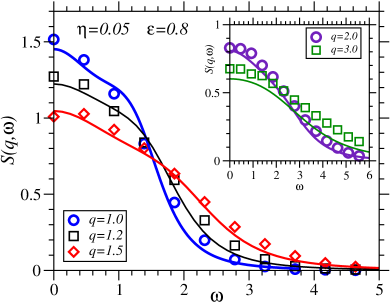
Figure 12: $S(q,\omega)$ for $\eta=0.05,\,\varepsilon=0.8$ and $q=1.0$ – $3.0$.

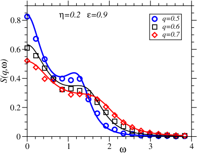
Figure 13: $S(q,\omega)$ for $\eta=0.2,\,\varepsilon=0.9$ and $q=0.5$ – $0.7$.

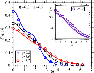
Figure 14: $S(q,\omega)$ for $\eta=0.2,\,\varepsilon=0.9$ and $q=0.8$ – $1.5$.

The corresponding best fit parameters are the transport coefficients $D_{T}$ and $\nu_{\mathrm{l}}$ which are shown graphically in Figs. 15 & 16. The fits require $q$-dependent transport coefficients because we consider wave numbers outside the hydrodynamic regime. It is difficult to estimate the hydrodynamic regime, but we need at least $q<q_{c}$ (see Table 2), corresponding to $D_{T}q^{2}<\frac{3\Gamma_{0}}{2T_{0}}$. For $\eta=0.2$, we are able to reach this regime and indeed find that $D_{T}$ and $\nu_{\mathrm{l}}$ are approximately independent of $q$. For $\eta=0.05$ even the smallest $q$ values are not in the hydrodynamic regime yet, and for $\eta=0.1$ the smallest wave numbers are in the crossover regime. As far as temperature fluctuations are concerned, the diffusive regime is restricted to larger wave numbers $D_{T}q^{2}>\frac{3\Gamma_{0}}{2T_{0}}$, so that $D_{T}$ can only be extracted from an intermediate range of $q$-values, such that $q>q_{c}$ but $q$ still small enough to ignore higher order terms in $q$. Again, for $\eta=0.2$ this seems possible, whereas for $\eta=0.05$ our data are not sufficient.

Tabulated in Table 2 is a quantitative comparison of the fit results for small $q$ with the theoretical predictions for $D_{T}=\frac{2\kappa}{dn}$ and $\nu_{\mathrm{l}}=\frac{1}{\rho}\left(\frac{2\eta_{\mathrm{shear}}(d-1)}{d}+\zeta\right)$, where $\eta_{\mathrm{shear}}$ and $\zeta$ are shear and bulk viscosity respectively. For the comparison with Brilliantov et al. we use Eqs. (20.13) & (20.30) of Ref. Brilliantov and Pöschel (2004) for $\eta_{\mathrm{shear}}$ and $\kappa$ respectively and $\zeta$ of Eq. (32) of Ref. Dufty et al. (1997). For the predictions of Dufty et al. we used Eqs. (29), (30) and (32) of Ref. Dufty et al. (1997) and for the predictions of Garzó et al. we used Eqs. (B1), (2.2), (3.8), (2.3) and (3.9) of Ref. Garzó et al. (2007).

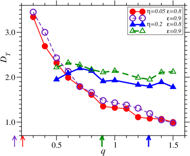
Figure 15: Thermal diffusivity $D_{T}(q)$ obtained via fits to $S(q,\omega)$ with Eq. (33). The arrows indicate the $q_{c}$ values from Table 1.

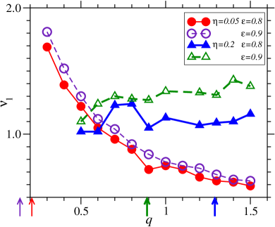
Figure 16: Longitudinal viscosity $\nu_{\rm l}(q)$ obtained via fits to $S(q,\omega)$ with Eq. (33). The arrows indicate the $q_{c}$ values from Table 1.

$\eta=0.05$
	$\varepsilon=0.8$		$\varepsilon=0.9$
	$D_{T}$	$\nu_{\rm l}$	$D_{T}$	$\nu_{\rm l}$
Fit Results: $q=0.2$	4.72	2.55	4.63	3.23
$q=0.3$	3.34	1.69	3.45	1.81
$q=0.4$	2.69	1.39	3.00	1.52
Brilliantov et al. Brilliantov and Pöschel (2004)	3.19	2.26	3.54	2.25
Dufty et al. Dufty et al. (1997)	4.71	2.82	4.07	2.77
Garzó et al. Garzó et al. (2007)	5.62	2.78	5.06	2.67
$\eta=0.1$
	$\varepsilon=0.8$		$\varepsilon=0.9$
	$D_{T}$	$\nu_{\rm l}$	$D_{T}$	$\nu_{\rm l}$
Fit Results: $q=0.3$	2.23	1.20	2.67	1.70
$q=0.4$	2.25	1.02	2.42	1.25
$q=0.5$	2.15	1.07	2.33	1.20
Brilliantov et al. Brilliantov and Pöschel (2004)	1.39	1.13	1.55	1.13
Dufty et al. Dufty et al. (1997)	2.67	1.69	2.42	1.71
Garzó et al. Garzó et al. (2007)	2.81	1.53	2.53	1.48
$\eta=0.2$
	$\varepsilon=0.8$		$\varepsilon=0.9$
	$D_{T}$	$\nu_{\rm l}$	$D_{T}$	$\nu_{\rm l}$
Fit Results: $q=0.5$	1.95	1.02	2.22	1.10
$q=0.6$	2.09	1.02	2.32	1.24
$q=0.7$	2.20	1.23	2.27	1.30
Brilliantov et al. Brilliantov and Pöschel (2004)	0.52	0.83	0.57	0.85
Dufty et al. Dufty et al. (1997)	2.03	1.63	2.01	1.72
Garzó et al. Garzó et al. (2007)	1.40	1.15	1.26	1.15

Table 2: Comparison of theoretical predictions and fit results for $D_{T}$ and $\nu_{\mathrm{l}}$.

We find best agreement between the simulation results for the smallest $q$ and the predictions of Dufty et al. Dufty et al. (1997) and fairly good agreement with the predictions of Garzó et al. Garzó et al. (2007).

Finally, we compare the speed of sound as obtained from the maximum of the current correlation with the predictions from the hydrodynamic theory in either the inelastic regime (see Eq. (27)) or the diffusive regime (see Eq. (29)). We find very good agreement (see Table 3) of the simulation results with Eq. (29), implying $D_{T}q^{2}\gg\frac{3\Gamma_{0}}{2T_{0}}$ and adiabatic sound propagation. However one should keep in mind that our procedure to extract the sound velocity from the maximum of the current correlation yields only an estimate of the sound velocity.

	via $\omega_{\mathrm{max}}(q)$	$D_{T}q^{2}\ll\frac{3\Gamma_{0}}{2T_{0}}$	$D_{T}q^{2}\gg\frac{3\Gamma_{0}}{2T_{0}}$
$\epsilon=0.8\quad\eta=0.05$	1.58	0.73	1.55
$\eta=0.1$	1.81	0.90	1.87
$\eta=0.2$	2.57	1.37	2.79
$\epsilon=0.9\quad\eta=0.05$	1.62	0.74	1.56
$\eta=0.1$	1.89	0.92	1.90
$\eta=0.2$	2.66	1.40	2.86

Table 3: The speed of sound, $c$, determined via the slope of the simulation results for $\omega_{\mathrm{max}}(q)$ (see Fig. 10) compared with the predicted values of Eq. (27) in the case of $D_{T}q^{2}\ll\frac{3\Gamma_{0}}{2T_{0}}$ and with Eq. (29) in the case of $D_{T}q^{2}\gg\frac{3\Gamma_{0}}{2T_{0}}$.

VII Conclusions and Outlook

We have investigated a homogeneously driven granular fluid of hard spheres at intermediate volume fractions $0.05\leq\eta\leq 0.4$ and for constant normal restitution coefficients $0.8\leq\varepsilon\leq 1.0$. Using event-driven simulations we have determined time-delayed correlation functions in the stationary state.

We find for the incoherent intermediate scattering function that it follows time-density superposition and that it is well approximated by the Gaussian $F_{\mathrm{incoh}}(\mathbf{q},t)=e^{\frac{-q^{2}}{6}\left\langle\Delta r^{2}(t)\right\rangle}$, where $\left\langle\Delta r^{2}(t)\right\rangle$ is the mean square displacement. The decay time of $F_{\mathrm{incoh}}(\mathbf{q},t)$ is rapidly increasing with increasing $\eta$, giving rise to a corresponding decrease of the diffusion constant. This precursor of a glass transition, which occurs at significantly larger $\eta$, is thus present not only in the elastic fluid but also in the inelastic case consistent with previous results at larger densities Kranz et al. (2010); Reis et al. (2007); Reyes and Urbach (2008).

We also determine the coherent intermediate scattering function $F(q,t)$, the longitudinal current correlation function $C_{\mathrm{l}}(q,t)$, and their Fourier transforms $S(q,\omega)$, $C_{\mathrm{l}}(q,\omega)$. Because we are interested in the long term dynamics we have simulated comparatively small systems of $N=10000$ particles and averaged over 100 independent simulation runs. We observe sound waves in the form of oscillations in $F(q,t)$ and estimate the sound velocity from the peak of $C_{\mathrm{l}}(q,t)$. For a quantitative comparison with the predictions of generalized fluctuating hydrodynamics, we use the linear hydrodynamic equations of Noije et al. van Noije et al. (1999) and fit the solutions thereof to the simulation results for $S(q,\omega)$. Depending on wave number and inelasticity the temperature fluctuations are predicted to be governed by inelastic collisions or diffusion van Noije et al. (1999); McNamara (1993). Our results are consistent with being in the “standard regime” van Noije et al. (1999) in which the speed of sound is the same as for elastic particles (see Table 3) and the damping of the sound wave depends on inelasticity. The most accurate fits were obtained assuming generalized hydrodynamic equations which account for both temperature diffusion as well as dissipation due to inelastic collisions (Eq. (33)). The resulting transport coefficients $D$, $D_{T}$ and $\nu_{\mathrm{l}}$ compare well with the predictions of Dufty et al. Dufty et al. (1997) and Garzó et al. Garzó et al. (2007).

We conclude that the time delayed correlations of a fluid of inelastically colliding particles are well described by generalized hydrodynamics. It would be interesting to extend our study in several directions. First, one would like to see still smaller $q$, requiring significantly larger systems (and yet also many independent runs for sufficient statistics). Second, it would be interesting to go to higher density and study sound propagation as the glass transition is approached. Finally, time- or frequency-dependent response functions are largely unexplored.