Nonequilibrium transport via spin-induced sub-gap states in superconductor/quantum dot/normal metal cotunnel junctions

Abstract

We study low-temperature transport through a Coulomb blockaded quantum dot (QD) contacted by a normal (N), and a superconducting (S) electrode. Within an effective cotunneling model the conduction electron self energy is calculated to leading order in the cotunneling amplitudes and subsequently resummed to obtain the nonequilibrium T-matrix, from which we obtain the nonlinear cotunneling conductance. For even occupied dots the system can be conceived as an effective S/N-cotunnel junction with subgap transport mediated by Andreev reflections. The net spin of an odd occupied dot, however, leads to the formation of sub-gap resonances inside the superconducting gap which gives rise to a characteristic peak-dip structure in the differential conductance, as observed in recent experiments.

I Introduction

Magnetic impurities in normal metals are known to give rise to so-called Abrikosov-Suhl resonances, Kondo64 ; Abrikosov65 ; Suhl65 which in turn lead to the celebrated Kondo conductance anomaly observed in normal (N/barrier/N) tunnel junctions with magnetic impurities in the barrier, Logan64 ; Wyatt64 ; Shewchun65 ; Appelbaum66 ; Anderson66 as well as in normal (N/QD/N) cotunnel junctions based on Coulomb blockaded quantum dots (QD) holding an odd number of electrons. Ng88 ; Glazman88 ; Goldhaber98 ; Cronenwett98 ; vanderWiel00 ; Nygaard00 Magnetic impurities in superconducting metals, on the other hand, give rise to localized Yu-Shiba-Rusinov bound states inside the superconducting gap, Yu65 ; Soda67 ; Shiba68 ; Rusinov69 ; Shiba69 which can be observed by measuring the local density of states (DOS) in scanning tunneling microscopy (STM) as sub-gap conductance peaks offset from the gap edge roughly by the magnitude of the exchange coupling (cf. Refs. Yazdani97, ; Salkola97, ; Flatte97, ; Flatte99, ; Balatsky06, ; Moca08, and references therein).

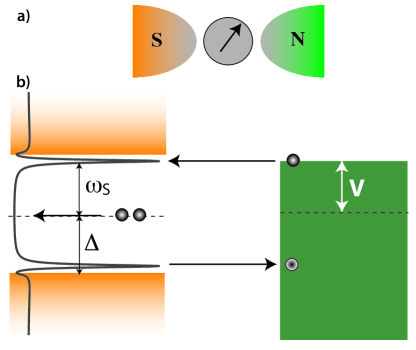
Figure 1: a) Sketch of the S/QD/N cotunnel junction comprised by a (gray) quantum dot holding a net spin, which is tunnel coupled to an (orange) superconducting and a (green) normal metal lead. b) Illustration of the basic Andreev reflection process giving rise to sub-gap transport and how it is enhanced by the presence of localized resonances induced by the spin on the quantum dot. The right (green) region illustrates the constant density of states (DOS) in the normal lead, shifted by the voltage $V$, and the left (orange) region illustrates the BCS DOS in the superconducting lead. The line is the local dot-electron DOS, with sub-gap resonances inside the gap and a pronounced dip at each gap edge.

In this paper, we explore the effects of spin-induced bound states in (S/QD/N) cotunnel junctions based on Coulomb blockaded quantum dots contacted to one superconducting and to one normal metal lead (cf. Fig. 1a). As we shall demonstrate, a coupling to the normal lead will broaden the localized bound states and the resulting scattering resonances will be reflected as characteristic sub-gap peaks, accompanied by pronounced dips at the gap edges in the nonlinear conductance. Basically, for a spinful quantum dot, sub-gap transport via Andreev reflections Andreev64 ; Blonder82 probes the profile of the sub-gap states rather than simply the bare BCS DOS (cf. Fig. 1b).

Transport measurements on such S/QD/N systems in the cotunneling regime have been already carried out. Graeber04 ; Deacon10a ; Deacon10b Most recently, Deacon et al. Deacon10a ; Deacon10b have indeed observed sub-gap conductance peaks for odd occupied S/InAs-QD/N devices, which they interpret as signatures of Andreev energy levels inside the gap. Tanaka07 ; Bauer07 Below, we argue that these peaks can be ascribed to Yu-Shiba-Rusinov resonances forming in a spinful cotunnel junction. This is consistent with the results of Refs. Tanaka07, ; Bauer07, , but allows for a simpler interpretation and calculation in terms of the Kondo model rather than the Anderson model. As we show, the experimental observation of enhanced Andreev current in spinful dots, conductance dips near the gap edges and gate-dependence of the sub-gap peak positions can all be explained in terms of such spin-induced resonances.

A number of works have addressed the problem of an Anderson impurity coupled to a single superconductor, either by numerical renormalization group (NRG) calculations Satori92 ; Bauer07 ; Hecht08 ; Lim08 or auxiliary boson methods, Clerk00 ; Sellier05 and have explored the intricate competition between Cooper-pairing and local correlations as a function of tunnel coupling $\Gamma$, charging energy $U$, and superconducting gap $\Delta$. Even a simple non-interacting ($U=0$) model gives rise to sub-gap states, Beenakker92 ; Khlus93 ; Bauer07 ; Hecht08 which may affect the nonlinear conductance, and sub-gap states are thus sustained in many different parameter regimes and possibly with many different characteristics. The present paper, however, focuses on quantum dots in the cotunneling regime safely inside a Coulomb diamond where charge fluctuations are strongly suppressed. Restricting ourselves to the cotunneling (Kondo) model, which is far simpler than the Anderson model, we retain crucial correlation features and, at the same time, we are able to capture the important physics of spin-induced bound states in a quantum dot setting, even out of equilibrium.

As already mentioned, a finite coupling to the normal metal lead will change the sub-gap bound states into broadened resonances but for low enough temperatures, Kondo correlations will become important and the resonances will be either suppressed, or supplemented by a Kondo resonance pinned to the normal metal Fermi surface. The full S/QD/N problem is an inherently complicated problem, Yamada10 ; Fazio98 ; Schwab99 ; Sun01 ; Cuevas01 ; Krawiec04 ; Domanski07 ; Domanski08 ; Tanaka07 ; Governale08 which we shall not attempt to solve here. In order to isolate and explore the observable consequences of the spin-induced sub-gap resonances, we neglect the log-singular terms arising from Kondo correlations with the normal lead, thus tacitly assuming the coupling between dot and normal lead to be sufficiently weak such that the corresponding Kondo temperature, $T_{K}$, is much smaller than than either temperature, $T$, or applied bias-voltage, $V$. Staying with an effective cotunneling model, it would indeed be interesting to investigate the competition between these sub-gap resonances and Kondo instabilities in the regime $\Delta\ll T_{K}$ where nonlinear conductance has been reported Graeber04 to be very different from the regime $\Delta\gg T_{K}$, which we study here.

After introducing the model, we explain how to get from lowest order self-energies to the current via the nonequilibrium T-matrix. Using this setup, we then start by investigating the case of a spinless even-occupied quantum dot, for which the effective cotunneling model takes the form of a simple potential scattering term. The nonlinear conductance is shown to be the same as for an ordinary S/N junction, Blonder82 ; Beenakker92 ; Cuevas96 which is to say that the spinless quantum dot can be viewed as an effective S/N-cotunnel junction.

Next, we treat the case studied originally by YuYu65 , ShibaShiba68 , and RusinovRusinov69 of a classical spin, modelled by a spin-dependent potential scattering term and determine again the nonlinear conductance. In this case we can still obtain exact analytical expressions for the current and comparing the expressions with the potential scattering case we find that already the classical spin leads to a peak below the gap accompanied by a square root dip at the gap edge (as opposed to the usual BCS square root divergence).

In contrast to the case of potential scattering and the classical spin approximation, which can be solved exactly, the full quantum mechanical spin is investigated by T-matrix resummed perturbation theory within leading order in the cotunneling amplitude. The numerically determined results for the nonlinear conductance are summarized in Fig. 2 for three different regimes of coupling asymmetry. For stronger coupling to the S-lead, resonances similar to the Yu-Shiba-Rusinov states below the gap are very sharp and the dip at the gap edge well defined. As the coupling to the normal lead increases, these resonances become broader and start filling-in the dip. Eventually the sub-gap resonances merge with the dip and reproduce the usual BCS-profile at the gap edge.

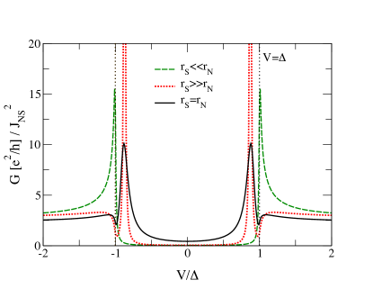
Figure 2: Comparison of the nonlinear conductance through an odd occupied quantum dot holding a net spin for different choices of coupling asymmetry. The spin exchange interaction is parametrized by $J_{\alpha\alpha^{\prime}}=J_{0}r_{\alpha}r_{\alpha^{\prime}}$. A spin-induced bound state is seen as a sub-gap resonance for strong coupling to the superconducting lead $r_{S}\gg r_{N}$ (factor of $10$ different) and for symmetric coupling, though broadened in that case. A dip appears at the superconducting gap, where one would expect a square root divergence like in the case of $r_{N}\gg r_{S}$, where the normal lead is stronger coupled.

II Model

II.1 Model system

We consider a quantum dot coupled to a normal and a superconducting lead (cf. Fig. 1a). The highest partially occupied orbital on the dot is represented by a single-orbital Anderson model:

$$H=H_{S}+H_{N}+H_{T}+H_{Dot},$$ (1)

with

$$H_{\alpha}= \sum_{\mathbf{k}\sigma}(\varepsilon_{k}-\mu_{\alpha})c^{\dagger}_{\alpha\mathbf{k}\sigma}c_{\alpha\mathbf{k}\sigma}$$

$$+\sum_{\mathbf{k}}(\Delta_{\alpha}^{\ast}c_{\alpha\mathbf{k}\uparrow}c_{\alpha-\mathbf{k}\downarrow}+\Delta_{\alpha}c_{\alpha-\mathbf{k}\downarrow}^{\dagger}c_{\alpha\mathbf{k}\uparrow}^{\dagger})\;,$$

$$H_{T}= \sum_{\alpha\mathbf{k}\sigma}\left(t_{\alpha}c_{\alpha\mathbf{k}\sigma}^{\dagger}d_{\sigma}+t_{\alpha}^{\ast}d_{\sigma}^{\dagger}c_{\alpha\mathbf{k}\sigma}\right),$$

$$H_{Dot}= \sum_{\sigma}\varepsilon_{d}d_{\sigma}^{\dagger}d_{\sigma}+Un_{d\uparrow}n_{d\downarrow},$$ (2)

where $\alpha=N,S$ labels respectively a normal metal electrode ($\Delta_{N}=0$) and a superconducting lead with an ordinary s-wave BCS DOS and a gap which is assumed to be real ($\Delta_{S}=\Delta$). This can be safely assumed, since the phase of the superconductor does not play a role in an S/N junction. Dot electrons of spin $\sigma$ are created by $d^{\dagger}_{\sigma}$ in an orbital of energy $\varepsilon_{d}$ and with a mutual Coulomb interaction strength $U$. The tunnelling amplitude between dot and electrodes is denoted by $t_{\alpha}$, and the Coulomb blockaded dot is tuned by the gate-voltage ($V_{g}\sim\varepsilon_{d}$) to hold a well-defined number of electrons. For a partial filling of this highest lying dot-orbital of one, i.e. a single electron on the dot, we thus assume that $\Gamma_{\alpha}=\pi\nu_{F}|t_{\alpha}|^{2}\ll\max(-\varepsilon_{d},\varepsilon_{d}+U)$.

In order to represent the exchange interaction between conduction electrons and the spinful quantum dot, it is necessary to augment the standard BCS Nambu-spinors to liberate the spin, from the charge. To this end, we introduce the four-spinors

$$\psi_{\alpha\mathbf{k}}^{\dagger} = \left(\begin{array}[c]{cccc}c_{\alpha\mathbf{k}\uparrow}^{\dagger},&c_{\alpha-\mathbf{k}\uparrow},&c_{\alpha\mathbf{k}\downarrow}^{\dagger},&c_{\alpha-\mathbf{k}\downarrow}\end{array}\right),$$ (4)

$$\psi_{\alpha\mathbf{k}} = \left(\begin{array}[c]{l}c_{\alpha\mathbf{k}\uparrow}\\ c_{\alpha-\mathbf{k}\uparrow}^{\dagger}\\ c_{\alpha\mathbf{k}\downarrow}\\ c_{\alpha-\mathbf{k}\downarrow}^{\dagger}\end{array}\right),$$ (9)

satisfying the anti-commutation relations

$$\{\psi_{\alpha\mathbf{k}\eta},\psi_{\alpha^{\prime}\mathbf{k}^{\prime}\eta^{\prime}}^{\dagger}\} = \delta_{\alpha\alpha^{\prime}}\delta_{\mathbf{k}\mathbf{k}^{\prime}}m_{\eta\eta^{\prime}}^{0},$$ (10)

$$\{\psi_{\alpha\mathbf{k}\eta}^{(\dagger)},\psi_{\alpha\mathbf{k}^{\prime}\eta^{\prime}}^{(\dagger)}\} = \delta_{\alpha\alpha^{\prime}}\delta_{-\mathbf{k}\mathbf{k}^{\prime}}m_{\eta\eta^{\prime}}^{c},$$ (11)

where we have introduced the following set of $4\times 4$ matrices:

$$m^{0} =\left(\begin{array}[c]{cccc}1&0&0&0\\ 0&1&0&0\\ 0&0&1&0\\ 0&0&0&1\end{array}\right),\qquad m^{a}=\left(\begin{array}[c]{cccc}1&0&0&0\\ 0&-1&0&0\\ 0&0&1&0\\ 0&0&0&-1\end{array}\right),$$ (20)

$$m^{b} =\left(\begin{array}[c]{cccc}0&0&0&-1\\ 0&0&1&0\\ 0&1&0&0\\ -1&0&0&0\end{array}\right),\qquad m^{c}=\left(\begin{array}[c]{cccc}0&1&0&0\\ 1&0&0&0\\ 0&0&0&1\\ 0&0&1&0\end{array}\right).$$ (29)

Within this notation, the Hamiltonian for the leads reads

$$H_{\alpha}=\frac{1}{2}\sum_{\mathbf{k}}\psi_{\mathbf{k}}^{\dagger}\ \xi_{\mathbf{k}}m^{a}\ \psi_{\mathbf{k}}+\frac{1}{2}\sum_{\mathbf{k}}\psi_{\mathbf{k}}^{\dagger}\ \Delta_{\alpha}m^{b}\ \psi_{\mathbf{k}}\;,$$ (30)

where $\alpha=S,N$, using $\Delta_{N}=0$ and $\Delta_{S}=\Delta$.

Since we focus entirely on cotunneling, we project out charge-fluctuations by means of a Schrieffer-Wolff transformation. Schrieffer66 ; Salomaa88 This simplifies the Anderson model to the effective cotunneling model:

$$H_{cotun}=H_{exch}+H_{pot},$$ (31)

with

$$H_{exch}=\frac{1}{4}\sum_{\alpha^{\prime}\mathbf{k}^{\prime}\eta^{\prime},\alpha\mathbf{k}\eta i}\ \sum_{i=x,y,z}\ J_{\alpha^{\prime}\alpha}S^{i}\psi_{\alpha^{\prime}\mathbf{k}^{\prime}\eta^{\prime}}^{\dagger}m_{\eta^{\prime}\eta}^{i}\psi_{\alpha\mathbf{k}\eta},$$ (32)

where the 4-spinor notation has been supplemented by the following augmentation of the Pauli matrices:

$$m^{x} =\left(\begin{array}[c]{cccc}0&0&1&0\\ 0&0&0&-1\\ 1&0&0&0\\ 0&-1&0&0\end{array}\right),\qquad m^{y}=\left(\begin{array}[c]{cccc}0&0&-i&0\\ 0&0&0&-i\\ i&0&0&0\\ 0&i&0&0\end{array}\right),$$ (41)

$$\qquad\qquad m^{z}=\left(\begin{array}[c]{cccc}1&0&0&0\\ 0&-1&0&0\\ 0&0&-1&0\\ 0&0&0&1\end{array}\right)\;.$$ (46)

The spin exchange interaction, Eq. (32), applies only to a spinful quantum dot holding a net spin, $\vec{S}=\frac{1}{2}d^{\dagger}_{\sigma^{\prime}}\vec{\tau}_{\sigma^{\prime}\sigma}d_{\sigma}$, whereas the potential scattering term

$$H_{pot}=\frac{1}{2}\sum_{\alpha^{\prime}\mathbf{k}^{\prime}\eta^{\prime},\alpha\mathbf{k}\eta}W_{\alpha^{\prime}\alpha}\psi_{\alpha^{\prime}\mathbf{k}^{\prime}\eta^{\prime}}^{\dagger}m_{\eta^{\prime}\eta}^{a}\psi_{\alpha\mathbf{k}\eta}\;,$$ (47)

applies to spinless quantum dots, as well as to spinful dots away from the particle-hole symmetric point in the middle of the relevant Coulomb blockade diamond. For a dot holding one electron, the two different cotunneling amplitudes are given by

$$J_{\alpha\alpha^{\prime}} =\frac{2Ut_{\alpha}t_{\alpha^{\prime}}^{*}}{(\varepsilon_{d}+U)(-\varepsilon_{d})},$$ (48)

and

$$W_{\alpha\alpha^{\prime}} =\frac{(2\varepsilon_{d}+U)t_{\alpha}t_{\alpha^{\prime}}^{*}}{2(\varepsilon_{d}+U)(-\varepsilon_{d})}\;,$$ (49)

where indeed $W_{\alpha\alpha^{\prime}}=0$ at the particle-hole symmetric point $\varepsilon_{d}=-U/2$. This result is readily generalized to any odd number of electrons on the dot, as long as only single-electron charge fluctuations are being eliminated by the Schrieffer-Wolff transformation. In the case of an even occupied dot, we denote the corresponding 2nd order cotunneling amplitude by $W_{\alpha\alpha^{\prime}}^{e}$.

As an illustrative intermediate step, we shall also discuss the case of a classical spin, where we replace the full exchange cotunneling term by a spin-dependent potential scattering term:

$$H_{exch}^{cl.}=\frac{1}{2}\sum_{\alpha^{\prime}\mathbf{k}^{\prime}\eta^{\prime},\alpha\mathbf{k}\eta}W_{\alpha^{\prime}\alpha}^{s}\psi_{\alpha^{\prime}\mathbf{k}\eta^{\prime}}^{\dagger}m_{\eta^{\prime}\eta}^{z}\psi_{\alpha\mathbf{k}\eta}\;.$$ (50)

We stress that this is merely a simplification of $H_{exch}$ corresponding to the limit of $J\to 0$ and $S\to\infty$, keeping the product, $JS$, constant. This was in fact the problem considered e.g by Shiba Shiba68 and as we shall demonstrate it already captures the essential physics of the spin-induced sub-gap resonances even for the full quantum spin.

II.2 Unperturbed Green functions

Since we want to study transport beyond the linear regime, we do the perturbation theory using Keldysh formalism. We define the contour-ordered conduction electron Green functions:

$$G_{\alpha\mathbf{k}\eta,\alpha^{\prime}\mathbf{k}^{\prime}\eta^{\prime}}(\tau,\tau^{\prime}) =-i\left\langle T_{C}\left\{\psi_{\alpha\mathbf{k}\eta}(\tau)\psi_{\alpha^{\prime}\mathbf{k}^{\prime}\eta^{\prime}}^{\dagger}(\tau^{\prime})\right\}\right\rangle.$$ (51)

In all expressions encountered below, the Green functions are summed over momentum. Therefore we start out by stating the unperturbed momentum summed Green functions for the leads. We have for the retarded and advanced Green functions

$$G^{(0),R/A}(\omega) =\sum_{\mathbf{k}}G^{(0),R/A}(\mathbf{k},\omega)$$

$$=-\pi\nu_{F}\theta(D-|\omega|)\frac{(\omega\pm i0^{+})m^{0}+\Delta m^{b}}{\sqrt{\Delta^{2}-(\omega\pm i0^{+})^{2}}},$$ (52)

where $D$ denotes the conduction electron half-bandwidth and we assume a constant DOS (pr. spin), $\nu_{F}$. For the spectral function, we then have

$$A^{(0)}(\omega) =2\pi\nu_{F}\theta(D-|\omega|)\theta(|\omega|-|\Delta|)\text{sign}(\omega)$$

$$\quad\times\frac{\omega m^{0}+\Delta m^{b}}{\sqrt{\omega^{2}-\Delta^{2}}}.$$ (53)

Notice that the anomalous part of the DOS is an odd function of $\omega$, which falls off as $\Delta/\omega$ for large $\omega$. For the normal lead, where $\Delta=0$, the spectral function reduces to

$$A_{N}^{(0)}(\omega) =2\pi\nu_{F}\theta(D-|\omega|)\;.$$ (54)

From the momentum-integrated spectral function, the lesser and greater Green functions are readily obtained as

$$G^{(0),<}(\omega) =iA(\omega)f(\omega),$$ (55)

and

$$G^{(0),>}(\omega) =-iA(\omega)(1-f(\omega)),$$ (56)

where $f$ denotes the Fermi function. The voltage is applied to the normal lead only, thus avoiding the complication with a running phase in the superconducting lead, and therefore the voltage $V$ enters only in the normal lead Green functions

$$G_{N,\eta\eta^{\prime}}^{(0),<} =if(\omega-m^{a}_{\eta\eta}V)m^{0}_{\eta\eta^{\prime}}A_{N}^{(0)}(\omega),$$ (57)

$$G_{N,\eta\eta^{\prime}}^{(0),>} =-i(1-f(\omega-m^{a}_{\eta\eta}V))m^{0}_{\eta\eta^{\prime}}A_{N}^{(0)}(\omega),$$ (58)

where the chemical potential shift has opposite sign for particle and hole components.

II.3 Current and T-matrix

Since we will be particularly interested in bound states (or resonances) as poles in the conduction electron T-matrix, it is convenient to express the current in terms of the T-matrix. To do this, we momentarily revert to the underlying Anderson model for which the current operator is found as the rate of change of the number of particles in the superconducting lead:

$$\hat{I} =\partial_{t}(Q_{S})=\frac{(-e)}{2i\hbar}\sum_{\mathbf{k}}[H_{T},\widehat{\psi}_{S\mathbf{k}}^{\dagger}m^{a}\widehat{\psi}_{S\mathbf{k}}].$$ (59)

Introducing four-spinors for the dot electrons:

$$\phi^{\dagger}=\left(\begin{array}[c]{cccc}d_{\uparrow}^{\dagger},&d_{\uparrow},&d_{\downarrow}^{\dagger},&d_{\downarrow}\end{array}\right),\;\;\;\;\;\;\;\phi=\left(\begin{array}[c]{l}d_{\uparrow}\\ d_{\uparrow}^{\dagger}\\ d_{\downarrow}\\ d_{\downarrow}^{\dagger}\end{array}\right),$$ (60)

the tunneling term takes the following form:

$$H_{T}=\frac{1}{2}\sum_{\alpha,\mathbf{k},\eta}t_{\alpha}m_{\eta\eta}^{a}\Big{(}\hat{\psi}_{\alpha\mathbf{k}\eta}^{\dagger}\phi_{\eta}+\phi_{\eta}^{\dagger}\hat{\psi}_{\alpha\mathbf{k}\eta}\Big{)},$$ (61)

where the tunneling amplitude has been chosen to be real, which is always possible for a single-level model with one normal lead, since a phase can be absorbed by a gauge transformation.

The expectation value of the current operator now involves the mixed $4\times 4$ Nambu Green functions, $i\langle T_{C}\psi_{S,\eta^{\prime}}(\tau)\phi^{\dagger}_{\eta}(\tau^{\prime})\rangle$, and one can show that

$$\langle\hat{I}\rangle =\frac{1}{2}\frac{e}{\hbar}\sum_{\gamma\eta}t_{S}^{2}m_{\gamma\gamma}^{a}\int\frac{d\omega}{2\pi}$$

$$\times\left(\big{[}G_{d;\eta\gamma}(\omega)G^{(0)}_{S;\gamma\eta}(\omega)\big{]}^{<}-\big{[}G^{(0)}_{S;\eta\gamma}(\omega)G_{d;\gamma\eta}(\omega)\big{]}^{<}\right),$$ (62)

where $G_{d;\eta\gamma}$ is the dot electron Green function in spinor space. In Eq. (62) we use the shorthand $[A(\omega)B(\omega)]^{<}=A^{R}(\omega)B^{<}(\omega)+A^{<}(\omega)B^{A}(\omega)$ implied by Langreth rules and subsequent Fourier-transformation. From equations of motion, the dot electron Green function can be obtained from the conduction electron T-matrix as

$$t_{\alpha}^{2}G^{R}_{d;\eta\eta^{\prime}}(t,t^{\prime}) =m_{\eta\eta}^{a}m_{\eta^{\prime}\eta^{\prime}}^{a}T^{R}_{\alpha;\eta\eta^{\prime}}(t,t^{\prime}),$$ (63)

which may be inserted to obtain the following formula for the current:

$$\langle I\rangle =\frac{e}{h}\sum_{\eta\gamma}m_{\eta\eta}^{a}\int\limits_{-\infty}^{\infty}d\omega\;{\mathrm{R}e}\Big{\{}[T_{S;\eta\gamma}(\omega)G^{(0)}_{S;\gamma\eta}(\omega)]^{<}\Big{\}},$$ (64)

where we have used the relation ${\cal G}^{<}_{\eta\eta^{\prime}}=-({\cal G}_{\eta^{\prime}\eta}^{<})^{\dagger}$. The current now relies solely on the conduction electron T-matrix, which we calculate within the effective cotunneling model derived from the Schrieffer-Wolff transformation. Thus the details of the quantum dot enter only via the interaction with the leads and in the following we study Eq. (64) for $H_{pot}$ and/or $H_{exch}$ as defined in section II.1.

The T-matrix effectively sums up an infinite repetition of the one-particle irreducible self energy $\Sigma$, which we obtain either exactly (for spinless dots and for the limit of a classical spin) or to leading order perturbation theory in the exchange cotunneling amplitude. In general, the retarded or advanced $SS$ component of the conduction electron T-matrix is found as

$$T_{SS}^{R/A}(\omega) =\Sigma^{R/A}_{SS,\mathrm{eff}}(\omega)\big{(}m^{0}-G^{(0),R/A}_{S}(\omega)\Sigma^{R/A}_{SS,\mathrm{eff}}(\omega)\big{)}^{-1},$$ (65)

with an effective $SS$ self energy which incorporates as well all processes going via the normal lead back into the superconducting lead:

$$\Sigma^{R/A}_{SS,\mathrm{eff}}(\omega)=\Sigma^{R/A}_{SS}(\omega)$$

$$\quad+\Sigma^{R/A}_{SN}(\omega)\big{[}[G_{N}^{(0),R/A}(\omega)]^{-1}-\Sigma^{R/A}_{NN}(\omega)\big{]}^{-1}\Sigma^{R/A}_{NS}(\omega).$$ (66)

This effective self energy also enters the Dyson equation for the interacting $SS$ Green function

$$G_{SS}^{R/A}(\omega) =\Big{\{}[G^{(0),R/A}_{S}(\omega)]^{-1}-\Sigma^{R/A}_{SS,\mathrm{eff}}(\omega)\Big{\}}^{-1}.$$ (67)

In the current formula Eq. (64), the lesser T-matrix enters through the following combination of Nambu matrices (omitting the $\omega$-dependence in the following):

$$T_{SS}^{<}G_{S}^{(0),A}+T^{R}_{SS}G_{S}^{(0),<}=T^{R}_{SS}G_{S}^{(0),<}+\Sigma^{<}_{SS,\mathrm{eff}}G^{A}_{SS}$$

$$\quad+T_{SS}^{R}\Big{(}G_{S}^{(0),<}\Sigma_{SS,\mathrm{eff}}^{A}+G_{S}^{(0),R}\Sigma_{SS,\mathrm{eff}}^{<}\Big{)}G_{SS}^{A}$$

$$\quad+T_{SN}^{R}\Big{(}G_{N}^{(0),<}\Sigma_{NS,\mathrm{eff}}^{A}+G_{N}^{(0),R}\Sigma_{NS,\mathrm{eff}}^{<}\Big{)}G_{SS}^{A},$$ (68)

where

$$\Sigma^{A}_{NS,\mathrm{eff}} =\Sigma^{A}_{NS}+\Sigma^{A}_{NN}(m^{0}-G^{(0),A}_{N}\Sigma^{A}_{NN})^{-1}G^{(0),A}_{N}\Sigma^{A}_{NS},$$ (69)

$$\Sigma^{<}_{\alpha\alpha^{\prime},\mathrm{eff}} =\Sigma_{\alpha\alpha^{\prime}}^{<}+\Sigma_{\alpha N}^{<}(m^{0}-G_{N}^{(0),A}\Sigma_{NN}^{A})^{-1}G_{N}^{(0),A}\Sigma_{N\alpha^{\prime}}^{A},$$ (70)

and

$$T_{SN}^{R} =\Big{(}m^{0}+T^{R}_{SS}G_{S}^{(0),R}\Big{)}\Sigma_{SN}^{R}\Big{(}m^{0}-G_{N}^{(0),R}\Sigma_{NN}^{R}\Big{)}^{-1}.$$ (71)

The irreducible self energy $\Sigma_{\alpha\alpha^{\prime}}$ depends on the details of the interacting system, thus determining the expressions for the T-matrix and the conductance as will be discussed now for the various cases.

III Results - Exactly solvable

III.1 Spinless dot - potential scattering

For a spinless dot, as for example one of even occupation with a singlet ground state, the effective cotunneling model has only the potential scattering term (47), and the irreducible conduction electron self energy is then exact already to first order in the potential scattering amplitude, $W^{e}_{\alpha\alpha^{\prime}}$:

$$\Sigma_{\alpha\eta,\alpha^{\prime}\eta^{\prime}}^{e} =\frac{1}{2}m^{a}_{\eta\eta^{\prime}}W^{e}_{\alpha\alpha^{\prime}}\;.$$ (72)

Since the self energy is independent of frequency, it has $\Sigma^{R}=\Sigma^{A}\equiv\Sigma^{e}$ and $\Sigma^{<}=0$, and the effective $SS$ Nambu matrix self energy therefore takes the following simple form:

$$\Sigma^{e,R/A}_{SS,\mathrm{eff}} =\frac{1}{\pi\nu_{F}}(\sigma_{r}^{e}\ m^{a}\mp i\sigma_{t}^{e}\ m^{0}),$$ (73)

where $\mp$ refers to retarded and advanced components and the real dimensionless coefficients are defined by

$$\sigma_{t}^{e} =\frac{\sigma^{e}_{SN}\sigma^{e}_{NS}}{1+(\sigma^{e}_{NN})^{2}},$$ (74)

$$\sigma_{r}^{e} =\sigma^{e}_{SS}-\sigma^{e}_{NN}\ \sigma_{t}^{e},$$ (75)

with the definition

$$\sigma_{\alpha\alpha^{\prime}}^{e}\equiv\frac{1}{2}\pi\nu_{F}W_{\alpha\alpha^{\prime}}^{e}.$$ (76)

Here $\sigma_{t}$ is responsible for transmission and $\sigma_{r}$ can be related to reflections back to the superconducting lead. Note that all expressions are in terms of the T-matrix $T_{SS}$ only. The T-matrix $T_{NN}$ cannot be written in the simple fashion of Eq. (73) since superconducting correlations are induced in the normal lead, whereas in $T_{SS}$ the coupling to normal lead only modulates the already present anomalous contributions in the superconducting lead.

If the normal lead was decoupled from the quantum dot, i.e. $W^{e}_{NS}=W^{e}_{SN}=0$, we would have no transport, i.e. $\sigma^{e}_{t}=0$, and $\sigma_{r}^{e}=\sigma_{SS}$. In the opposite limit where there are no reflections, i.e. $W^{e}_{SS}=W^{e}_{NN}=0$, the system becomes equivalent to a tunnel junction, with $\sigma_{r}^{e}=0$ and $\sigma_{t}^{e}=\sigma_{NS}\sigma_{SN}$. In general, however, the cotunnel junction studied here involves both numbers, $\sigma^{e}_{t/r}$. Even though the self energy is exact in this case, it should be kept in mind that the validity of our initial Schrieffer-Wolff transformation relies on the fact that the four dimensionless numbers, $\sigma_{\alpha\alpha^{\prime}}$, are all much smaller than one.

Inserting the above self energy (73) into Eqs. (68-71) and using current formula (64), we can now obtain a closed analytical expression for the nonlinear conductance at zero temperature. For voltages outside the gap, $V>\Delta$, we have

$$\frac{dI}{dV} =\frac{2e^{2}}{h}\frac{4\sigma_{t}^{e}}{\mathcal{D}^{e}_{V>\Delta}},$$ (77)

with the denominator defined as:

$$\mathcal{D}^{e}_{V>\Delta} =2\sigma_{t}^{e}+(1+(\sigma_{t}^{e})^{2}+(\sigma_{r}^{e})^{2})\ \sqrt{1-(\Delta/V)^{2}}.$$ (78)

For voltages inside the gap, $V<\Delta$, we have instead

$$\frac{dI}{dV} =\frac{4e^{2}}{h}\frac{4(\sigma_{t}^{e})^{2}}{\mathcal{D}^{e}_{V<\Delta}},$$ (79)

with denominator

$$\mathcal{D}^{e}_{V<\Delta} =(1+(\sigma_{t}^{e})^{2}+(\sigma_{r}^{e})^{2})^{2}(1-(V/\Delta)^{2})$$

$$\qquad+4(\sigma_{t}^{e})^{2}(V/\Delta)^{2}.$$ (80)

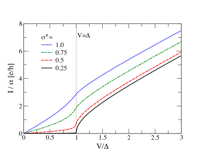
Figure 3: Current $I/\alpha$ for the spinless dot (even occupation) with equal dimensionless cotunneling amplitudes to S and N given by respectively $\sigma^{e}\equiv\pi\nu_{F}W^{e}/2=1,0.75,0.5,0.25$, corresponding to a cotunnel junction transmission of $\alpha=0.8,0.56,0.2,0.015$. Dotted line indicates the superconducting gap $V=\Delta$.

In the limit of $\Delta\to 0$ or $V\to\infty$, the differential conductance reaches the value $\frac{2e^{2}}{h}\alpha$, with a cotunnel junction transmission

$$\alpha =\frac{4\sigma_{t}^{e}}{(1+\sigma_{t}^{e})^{2}+(\sigma_{r}^{e})^{2}}\;,$$ (81)

which differs from that of a tunnel junction Cuevas96 ; Blonder82 merely by the presence of the reflection terms $W^{e}_{SS}$ and $W^{e}_{NN}$ comprising $\sigma_{r}^{e}$. Note that a rewriting of the full nonlinear conductance, (77-80), in terms of this $\alpha$ makes it identical to the expression found in Ref. Cuevas96, for a tunnel junction, and to the one by BTK Blonder82 , when expressing their barrier parameter $Z$ in terms of the transmission, $Z^{2}=\alpha^{-1}-1$.

The conductance at $V=\Delta$ is exactly $4e^{2}/h$, whereas the zero-bias conductance is given by

$$\frac{dI}{dV}\Big{|}_{V=0} =\frac{4e^{2}}{h}\left(\frac{2\sigma_{t}^{e}}{1+(\sigma_{t}^{e})^{2}+(\sigma_{r}^{e})^{2}}\right)^{2},$$ (82)

which agrees with the general result for the linear conductance of an N/S interface Beenakker92 : $G=4e^{2}/h\ \alpha^{2}/(2-\alpha)^{2}$, valid for any transmission $\alpha$.

Sub-gap transport for $V<\Delta$ is allowed by Andreev scattering processes, which proliferate with increasing cotunneling amplitudes $W^{e}_{\alpha\alpha}$. This is clearly seen in Fig. 3 where we plot the I-V curves for different tunneling amplitudes. The corresponding nonlinear conductances are shown in Fig. 4 and seen to simply reflect the BCS DOS for the smallest chosen tunneling amplitude.

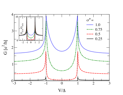
Figure 4: Differential conductance $G=dI/dV$ for the even dot with same parameters as in Fig. 3. Inset: the nonlinear conductance $G_{S/N}$ normalized by the value of $G_{N/N}=2e^{2}/h\ \alpha$.

III.2 Classical spin - spin dependent potential scattering

We commence with an extension of the spinless dot, described by a potential scattering term $W^{e}$, to a dot holding a classical spin, which we describe by Eq. (50) in terms of a spin-dependent potential scattering term $W^{s}$. In this case, the exact irreducible self energy is given by

$$\Sigma_{\alpha\eta,\alpha^{\prime}\eta^{\prime}}^{s} =\frac{1}{2}m^{z}_{\eta\eta^{\prime}}W^{s}_{\alpha\alpha^{\prime}}\;.$$ (83)

In line with the spinless case, the effective $SS$ self energy can be written as

$$\Sigma^{s,R/A}_{SS,\mathrm{eff}} =\frac{1}{\pi\nu_{F}}(\sigma_{r}^{s}\ m^{z}\mp i\sigma_{t}^{s}\ m^{0})\;,$$ (84)

where the same definitions (74) and (75) apply to the dimensionless coefficients, $\sigma_{t/r}$, when simply replacing $W^{e}_{\alpha\alpha^{\prime}}$ by $W^{s}_{\alpha\alpha^{\prime}}$. Note that the spin symmetry is broken by $m^{z}$ in contrast to the potential scattering case.

As before, we can find a closed expression for the nonlinear conductance at zero temperature. In Figs. 5 and 6 we first show the resulting I-V curves and corresponding nonlinear conductance for the same coupling strengths as used for the spinless case in Figs. 3-4. We limit the plots to the case of symmetric couplings and return to investigate asymmetric couplings for the full quantum mechanical spin in the next section. For weak coupling, the conductance in Fig. 6 is similar to the potential scattering case and merely reflects the BCS density of states. For increasing coupling strength a sub-gap peak appears symmetrically around zero bias and the conductance peak at $V=\Delta$ changes to a dip, as discussed below. As the peak moves closer to zero energy, it also becomes broader for our choice of symmetrically coupled leads. Note that for very strong coupling the two Yu-Shiba-Rusinov states mix and one sees only a broad peak centered at zero voltage, which we should emphasize has nothing to do with a Kondo resonance. All of these features can be identified in the following analytical formulas for the nonlinear conductance.

As in the case of potential scattering we find for the classical spin exact expressions for the differential conductance from perturbation theory. For voltages outside the gap, $V>\Delta$, we have

$$\frac{dI}{dV} =\frac{2e^{2}}{h}\ 4\sigma_{t}^{s}\ \frac{\mathcal{D}_{V>\Delta}^{s}}{4(\sigma_{r}^{s})^{2}(\Delta/V)^{2}+\big{(}\mathcal{D}_{V>\Delta}^{s}\big{)}^{2}},$$ (85)

with $\mathcal{D}_{V>\Delta}^{s}$ given by (78) with $\sigma^{e}$ replaced by $\sigma^{s}$. In the limit $\Delta\to 0$ or $V\to\infty$ we find again that the conductance is given by $2e^{2}/h\ \alpha$ with the cotunnel junction transmission, Eq. (81), in terms of $\sigma_{t/r}^{s}$. However, due to the term with $\sigma_{r}^{s}$ in the denominator, the differential conductance here cannot be expressed in terms of $\alpha$ alone.

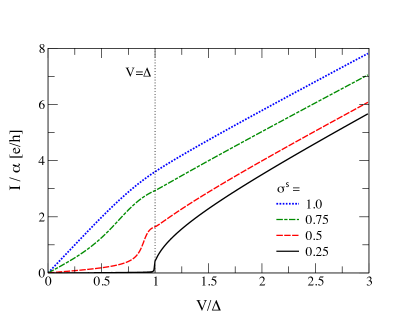
Figure 5: Current $I/\alpha$ for a symmetrically coupled quantum dot occupied by an odd number of electron where the spin is treated classically. The coupling strengths are chosen $\sigma^{s}\equiv\pi\nu_{F}W^{s}/2=1,0.75,0.5,0.25$ similarly to Fig. 3.

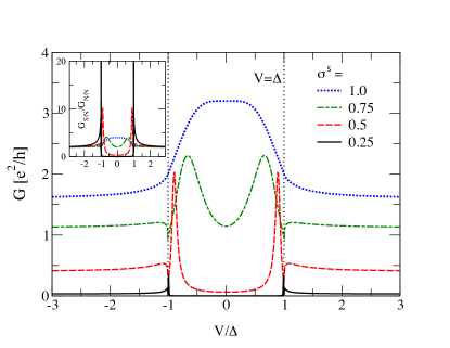
Figure 6: Differential conductance $G=dI/dV$ for the odd occupied dot with a classical spin where the coupling strengths are the same as in Fig. 5. Inset: Conductance $G_{S/N}$ normalized by $G_{N/N}=2e^{2}/h\ \alpha$.

For $\sigma_{r}^{s}\approx 0$, i.e. weak coupling to the superconducting lead $\sigma_{SS}\approx 0$, the conductance outside the gap is identical to that in the spinless case with a BCS-like square root singularity at $|eV|\approx\Delta$. This changes rapidly with increasing $\sigma_{r}^{s}$, which changes the singularity at $|eV|=\Delta$ into a dip with a square root increase with voltage (cf. Figs. 5 and 6). At $V=\Delta$ the differential conductance takes the value

$$\frac{dI}{dV}\Big{|}_{V=\Delta} =\frac{4e^{2}}{h}\frac{(\sigma_{t}^{s})^{2}}{(\sigma_{r}^{s})^{2}+(\sigma_{t}^{s})^{2}},$$ (86)

which reaches the $4e^{2}/h$, attained in the spinless case, when $\sigma_{r}^{s}\ll\sigma_{t}^{s}$, i.e. in the case where the dot is coupled much stronger to the normal, than to the superconducting lead. On the contrary, for strong coupling to the superconducting lead, $\sigma_{r}^{s}\gg\sigma_{t}^{s}$, the value of the conductance is suppressed and the dip is clearly visible.

The spectral weight which has been removed at the gap edge can instead be found inside the gap. For voltages inside the gap, $V<\Delta$, the conductance takes the following form:

$$\frac{dI}{dV} =\frac{4e^{2}}{h}\Big{(}2V^{2}-\Delta^{2}+\frac{\Delta^{2}}{4(\sigma_{r}^{s})^{2}}\mathcal{D}_{V<\Delta}^{s}\Big{)}$$

$$\qquad\times\frac{\Gamma_{S}}{(V-\omega_{S})^{2}+\Gamma_{S}^{2}}\frac{\Gamma_{S}}{(V+\omega_{S})^{2}+\Gamma_{S}^{2}},$$ (87)

where

$$\omega_{S} =\pm\Delta\frac{1-((\sigma_{r}^{s})^{2}+(\sigma_{t}^{s})^{2})^{2}}{(1+(\sigma_{r}^{s})^{2}-(\sigma_{t}^{s})^{2})^{2}+4(\sigma_{r}^{s})^{2}(\sigma_{t}^{s})^{2}}\;,$$ (88)

$$\Gamma_{S} =\Delta\frac{4\sigma_{r}^{s}\sigma_{t}^{s}}{(1+(\sigma_{r}^{s})^{2}-(\sigma_{t}^{s})^{2})^{2}+4(\sigma_{r}^{s})^{2}(\sigma_{t}^{s})^{2}}\;.$$ (89)

The sub-gap conductance shows two peaks of approximately Lorentzian form, centered at energies $\pm\omega_{S}$ and having a width of $\Gamma_{S}$. In the case of vanishing coupling to the normal lead, i.e. $\sigma_{t}^{s}=0$ and $\sigma_{r}^{s}=\sigma_{SS}^{s}$, the resonances sharpen to form real bound states, located at:

$$\omega_{S} =\pm\Delta\frac{1-(\sigma_{r}^{s})^{2}}{1+(\sigma_{r}^{s})^{2}}.$$ (90)

This limit reproduces the case of a classical spin embedded in a bulk superconductor.Yu65 ; Soda67 ; Shiba68 ; Rusinov69 . For weak coupling this bound state is thus offset from the superconducting gap by roughly the interaction strength. For strong coupling the dependence changes, but interactions of the order of the band width will on the other hand conflict with the confinement of electrons on the quantum dot. The classical spin case is artificial in the sense that the spin symmetry is broken although the spin exchange interaction does not break this symmetry. In the next section it is shown that spin-induced sub-gap bound states, qualitatively similar to those found in this section, are still present if the spin is treated quantum mechanically.

IV Results - Quantum spin

IV.1 Exchange cotunneling

Whereas the calculation for the classical spin is exact, we have to rely on leading order perturbation theory when it comes to calculating the conduction electron self energy in the case of exchange cotunneling with a quantum mechanical spin. For zero magnetic field, the leading term in the conduction electron self energy is of second order in the exchange interaction:

$$\Sigma_{\alpha\eta,\alpha^{\prime}\eta^{\prime}}(t-t^{\prime})= \frac{1}{16}\sum_{\gamma,\gamma^{\prime}}\sum_{ij}\langle S^{i}(t)S^{j}(t^{\prime})\rangle_{(0)}m_{\eta\gamma}^{i}m_{\gamma^{\prime}\eta^{\prime}}^{j}$$

$$\times\sum_{\alpha^{\prime\prime}}J_{\alpha\alpha^{\prime\prime}}^{\eta\gamma}G_{\alpha^{\prime\prime},\gamma\gamma^{\prime}}^{(0)}(t-t^{\prime})J_{\alpha^{\prime\prime}\alpha^{\prime}}^{\gamma^{\prime}\eta^{\prime}}\;.$$ (91)

Before presenting the general results, let us first take a look at the limit of negligible coupling to the normal lead, i.e. $J_{NS}\approx 0$. With the experience from last section, we expect to find bound states showing up as zeros in the denominator of the T-matrix. These are located at energies $\omega_{S}$ for which

$$0 =\mathrm{det}\Big{\{}[G^{(0),R/A}_{S}(\omega_{S})]^{-1}-\Sigma^{R/A}_{SS}(\omega_{S})\Big{\}},$$ (92)

and inserting the self energy (91), we can identify bound states at energies

$$\omega_{S} =\pm\Delta\frac{1-3/4\,g_{SS}^{2}}{1+3/4\,g_{SS}^{2}}\;.$$ (93)

in terms of the dimensionless exchange cotunneling amplitude

$$g_{SS}=\frac{1}{4}\pi\nu_{F}J_{SS}\;.$$ (94)

Expression (93) is also valid for the general case of a spin exchange interaction (32) with a higher spin (e.g. spin-$1$ in an even dot) by replacing $3/4$ with $S(S+1)$.

The bound state energies in Eq. (93) match those found for the classical spin (90) (in the limit of vanishing coupling to the normal lead) if one replaces $W^{s}_{SS}$ by $\sqrt{3}/4\,J_{SS}$. However, this analogy to the classical (or polarized) spin case does not hold anymore when the coupling to the normal lead is non-zero. We shall return to this comparison in Section IV.2.

As for the classical spin, a finite coupling to the normal lead broadens the bound states into resonances. Unlike for the classical spin, however, we cannot give a closed analytical expression for the T-matrix nor for the nonlinear conductance.

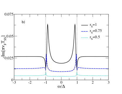
Figure 7: Imaginary part of the T-matrix, - Im$[\pi\nu_{F}T_{SS}]$, for a spinful quantum dot asymmetrically coupled to a superconducting and normal lead with $g_{0}\equiv\pi\nu_{F}J_{0}/4=0.3$ leading to $\omega_{S}\approx 0.8735\Delta$ for $r_{N}=0$; a) $r_{S}=1$ is kept constant and the coupling to the normal lead $r_{N}$ is changed; b) $r_{N}=1$ is kept constant and the coupling to the superconducting lead is reduced.

To obtain the retarded T-matrix, we insert (91) into (65) and (66). The imaginary part of the T-matrix, which is proportional to the local DOS on the dot (cf. Eq. (63)), is plotted in Fig. 7. We parametrize the exchange cotunneling amplitudes from Eq. (48) by $J_{\alpha\alpha^{\prime}}=J_{0}r_{\alpha}r_{\alpha^{\prime}}$, where $J_{0}=4g_{0}/\pi\nu_{F}$ and $r_{\alpha}=t_{\alpha}/t_{0}$ is the ratio between the tunneling amplitude to lead $\alpha=S,N$ and $t_{0}=\max\{t_{N},t_{S}\}$.

The spin-induced sub-gap resonance is seen to stay at the same position as long as the coupling to the superconducting lead is stronger than the coupling to the normal lead, i.e. $1=r_{S}\geq r_{N}$ in Fig. 7a. The peak though gets broader and lower with increasing coupling, $r_{N}$, to the normal lead. In Fig. 7b we show the behavior when the spin is stronger coupled to the normal lead by reducing the coupling to the superconducting lead $1=r_{N}\geq r_{S}$. Besides a strong suppression of the overall value, we also observe that the resonance moves out towards the gap edge and, for very weak coupling to the superconducting leads, eventually gives back spectral weight to reconstruct the usual square root divergence at the superconducting gap $\Delta$. These characteristics will be present again in the nonlinear conductance through the quantum dot as discussed later on in this section.

IV.1.1 Gate dependence of the spin-induced sub-gap resonance energy

At the particle-hole symmetric point, $\varepsilon_{d}=-U/2$, the spinful dot derived from the Anderson model has no potential scattering term, i.e. $W=0$ at this point (cf. Eq. (49)). Leaving this point by adjusting the gate-voltage (which is proportional to $\varepsilon_{d}$), however, the potential scattering term has to be included, and it is clear from Eqs. (48-49) that both $J$ and $W$ will in fact increase in magnitude until eventually the Schrieffer-Wolff transformation breaks down as one comes too close to a charge-degeneracy point for the Coulomb blockaded quantum dot.

To investigate the dependence of the resonance frequency, $\omega_{S}$, on gate-voltage, we again consider the case where the dot is coupled only to the superconducting lead. As before, this is found as a root for the denominator in the T-matrix (cf. Eq. (92)), but now we have to include also the first order term from potential scattering, $\Sigma^{(1)}=W_{\alpha\alpha^{\prime}}m^{a}/2$, in the irreducible self energy. Doing this, one finds that the T-matrix pole will be located at

$$\omega_{S} =\pm\Delta\sqrt{\frac{(1-3/4\,g_{SS}^{2})^{2}+w_{SS}^{2}}{(1+3/4\,g_{SS}^{2})^{2}+w_{SS}^{2}}}\;,$$ (95)

where $w_{SS}=\pi\nu_{F}W_{SS}/2$. For $w_{SS}=0$ and $S=1/2$, we thus reproduce Eq. (93) for a spin coupled to a superconductor and for $g_{SS}=0$ we find $\omega_{S}=\pm\Delta$, i.e. no spin-induced sub-gap state if there is no exchange coupling and only potential scattering as discussed in section III.1.

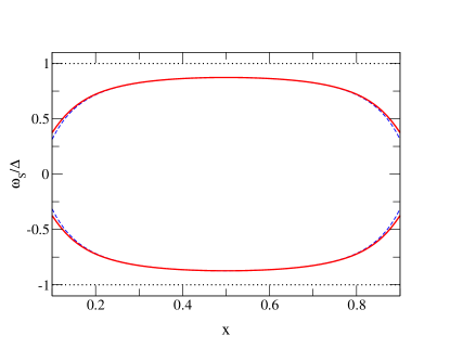
Figure 8: Gate dependence of the spin-induced sub-gap resonance $\omega_{S}/\Delta$ in terms of $x=|\epsilon_{d}|/U$, and with $g_{SS}=0.3$; red (full) line including potential scattering and blue (dashed) line without. Black (dotted) line indicates the energy of the superconducting gap.

In Fig. 8 we show how the position of the sub-gap state changes inside the Coulomb diamond as a function of $x=|\epsilon_{d}|/U$. As the coupling strength defined in Eq. (48) increases towards the edges of the diamond (i.e. $x=0$ and $x=1$), the bound state moves closer to zero. At the same time we of course expect the width of the peak to increase both due to the added influence of the potential scattering term but first and foremost due to the increase in cotunneling amplitudes as one moves away from the particle-hole symmetric point ($x=1/2$). Notice that the potential scattering term, with the gate dependence as defined in Eq. (49), makes practically no difference until perturbation theory breaks down anyway. Interestingly, the gate dependence shown in Fig. 8 is very similar to that reported in recent experiments on N/QD/S Deacon10a and S/QD/S junctions. Grove09

For the rest of the paper we solely deal with the particle-hole symmetric point where the potential scattering is zero.

IV.2 Transport via spin-induced sub-gap resonances

To derive the nonlinear conductance in the case of a quantum mechanical spin, we need to include the full Keldysh matrix structure in Eq. (64) and (68). Therefore we cannot provide an analytic expression for this case, but the calculations are straightforward and do not need extensive numerical effort.

We can distinguish between a hierarchy of contributions in Eq. (68). Summing over $m^{a}_{\eta\eta}$ in Eq. (64), $T^{R}_{SS}G^{(0),<}_{S}$ cancels out while $\Sigma_{SS,eff}^{<}G_{SS}^{A}$ contributes to the current already to second order in the spin exchange interaction $J_{\alpha\alpha^{\prime}}$. This is the dominant contribution in the conductance as illustrated in Fig. 9.

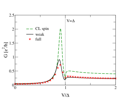
Figure 9: Comparison of the differential conductance through a spinful quantum dot, treated quantum mechanically, taking into account all terms (red data points) or the the weak coupling term only (black line) for symmetric coupling $r_{S}/r_{N}=1$ and $g_{0}=0.3$ . Furthermore, conductance treating the spin classically, dashed (green) line, with a coupling of $W^{s}_{\alpha\alpha^{\prime}}=\sqrt{3}/4\ \sqrt{J_{\alpha\alpha^{\prime}}}$.

There “weak coupling” refers to calculating the nonlinear conductance including $\Sigma_{SS,eff}^{<}G^{A}_{SS}$ only, while “full” refers to including furthermore all contributions in Eq. (68) which are of fourth order in lowest order in $J_{\alpha\alpha^{\prime}}$. As can be seen in Fig. 9, the weak coupling term actually overestimates the height of the spin-induced sub-gap resonance and the value at the edge of the superconducting gap slightly. However, for the coupling $g_{0}=0.3$ (cf. Fig. 9) studied in the following, this provides a very good approximation and therefore Figs. 10-13 are calculated with the contribution from $\Sigma_{SS,eff}^{<}G_{SS}^{A}$ only. For stronger coupling the deviation is more severe. Furthermore, Kondo correlation effects have to be taken into account for strong coupling to the normal lead and this regime is not discussed here.

Fig. 9 also shows a comparison with the conductance in the case of a spin treated classically. For symmetrically coupled junctions we find that $W^{s}_{\alpha\alpha^{\prime}}=\sqrt{3}/4\ \sqrt{J_{\alpha\alpha^{\prime}}}$ provides a reasonable agreement although the energy of the spin-induced sub-gap state is slightly shifted and the value of the conductance is in general overestimated. Whereas a linear relation, $W^{s}_{SS}=\sqrt{3}/4\ J_{SS}$, is a good approximation for a spin decoupled from the normal lead, a square root dependence ($W^{s}_{\alpha\alpha^{\prime}}=\sqrt{3}/4\sqrt{J_{\alpha\alpha^{\prime}}}$) fits the quantum mechanical case for symmetrically coupled junctions. In practise, we can always find a value for the classical spin case, which fits rather well the full spin-flip scattering case, but (as already clear from the two simple limiting cases) there is no obvious systematics involved and the value is strongly dependent on asymmetry and strength of the coupling to the leads. Nevertheless, we claim that the classical spin case provides good qualitative insight into the problem of a spin coupled to a superconductor.

Since the conductance is directly related to the local DOS, i.e. Im$[G^{A}_{SS}]$, it is not surprising, that sub-gap states are observed in the transport through an N/QD/S cotunnel junction. As already illustrated in Fig. 1, the local DOS of the superconductor is probed by Andreev scattering processes to the normal lead. The enhanced spectral density at the energy of the spin-induced sub-gap state leads to a sub-gap peak in the differential conductance and a reduced DOS at the superconducting gap $\Delta$ as reflected in $dI/dV$.

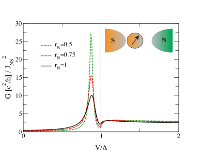
Figure 10: Differential conductance $G=dI/dV$ for increasing coupling to normal lead, $r_{S}=1$ and $g_{0}=0.3$. The conductance is renormalized by the “transport” coupling strength, $J_{NS}^{2}$, across the dot in order to compare the different curves. Inset: Illustration of a spin state coupled to the superconducting lead, thus forming a bound state, which is probed by the normal lead.

Comparing Figs. 10 and 11 with Fig. 7 we find significant agreement, since Im$[T^{R}_{SS}]$ is (besides a prefactor proportional to the interaction) given by the interacting local DOS.

As shown in Fig. 10 the spin-induced sub-gap state stays at roughly the same energy $\omega_{S}$ given by Eq. (93) (for a spinful quantum dot decoupled from the normal lead) as long as the superconducting lead is stronger coupled to the dot than the normal lead, $r_{S}\geq r_{N}$. This can be understood schematically as illustrated in the inset of Fig. 10: If the spin is coupled strongly to the superconducting lead, a bound state is created and can be probed in transport through the N/S setup with a weakly coupled normal lead.

On the contrary, if the normal lead is stronger coupled to the impurity, $r_{N}\gg r_{S}$, we only probe the BCS superconducting DOS (i.e. no spin-induced sub-gap resonances).

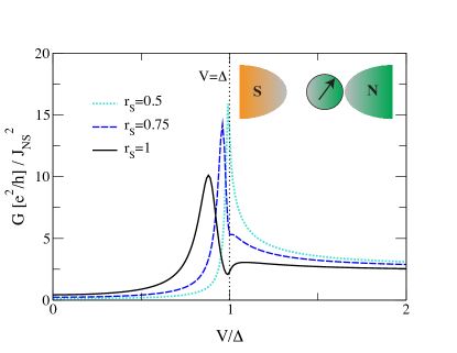
Figure 11: Renormalized nonlinear conductance $G/J_{NS}^{2}$ for increasing coupling to the superconducting lead and $r_{N}=1$; Inset: Illustration of a spin state strongly coupled to the normal lead and thus only the superconducting DOS is probed in transport.

This is sketched in the inset of Fig. 11. Starting from a nonlinear conductance displaying a clear sub-gap peak for $r_{N}=r_{S}$, the resonance moves closer towards the energy of the superconducting gap $\Delta$ as the coupling to the normal lead is increased, $r_{N}>r_{S}$ in Fig. 11. If the coupling to the normal lead dominates, no sub-gap resonance can be distinguished from the square-root singularity at $\Delta$. As was also illustrated in Fig. 2 and is shown again in Figs. 10 and 11 an experiment of the transport through an N/QD/S junction can therefore have very different signatures depending on the asymmetry of the coupling.

It is expected from the expression of $\omega_{S}$, (93), that the spin-induced sub-gap bound state moves into the gap for increasing coupling strength. This is illustrated in Fig. 12 choosing symmetric coupling to the superconducting and normal lead.

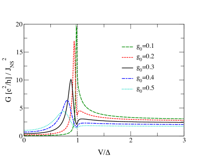
Figure 12: Renormalized differential conductance $G/J_{NS}^{2}$ for increasing coupling strength, $g_{0}=0.1,0.2,0.3,0.4,$ and $0.5$, where both leads are symmetrically coupled, $r_{N}=r_{S}=1$.

For $g_{0}=0.1$ the sub-gap resonance state is present, but hidden at $V=\Delta$. However, already for $g_{0}=0.2$ the conductance is seen to change into a peak at $\omega_{S}\approx 0.94\Delta$ and an associated dip at $\Delta$ instead of the square root divergence of the clean superconducting DOS. Note that the conductance value at $\Delta$ decreases with increasing coupling to the superconducting lead. Since we have chosen symmetric coupling in Fig. 12, the increasing coupling to the normal lead causes a concomitant life time broadening of the peak inside the gap similar to the case of a classical spin.

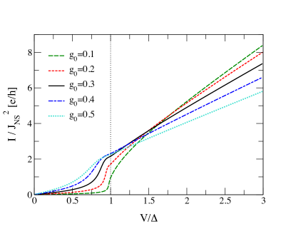
Figure 13: Renormalized current $I/J_{NS}^{2}$ for the same parameters as Fig. 12.

Finally, Fig. 13 shows the current for the same parameters as the conductance in Fig. 12. The dip in the conductance at the superconducting gap is hardly visible in the current, where it should show up as a kink. Most interestingly, the current has a sharp increase at the energy of the spin-induced sub-gap resonance $\omega_{S}$. This could easily be misinterpreted as a reduced superconducting gap $\Delta$, since there is no obvious difference between the line shapes of the curves with $g_{0}=0.1$ and $g_{0}=0.4$ in Fig. 13. Therefore, a clear distinction between a reduced superconducting gap and a spin-induced sub-gap resonance signature is best seen in the differential conductance.

V Summary and discussion

We have investigated the transport characteristics of a Coulomb blockaded quantum dot sandwiched between a normal and a superconducting lead. The focus has been on the difference between a dot with an even number of electrons and one with an odd number of electrons or, in more general terms, the difference between dots with zero or finite spin.

We have restricted the calculations to the cotunneling regime, where charge fluctuations are strongly suppressed. The effective model is in this situation a ”cotunnel junction”, where for even occupancy (or a spinless dot) one obtains a simple tunneling Hamiltonian for tunneling between N and S, plus reflection terms (N to N, and S to S). In the language of the Schrieffer-Wolff transformation, this is known as potential scattering, see Eq. (47). In contrast, for odd occupancy (or a spinful dot) there is an additional term, namely the Kondo, or exchange-cotunneling, Hamiltonian, see Eq. (32), where the tunneling electrons couple to the spin on the dot and hence may induce spin flips. Furthermore, at the particle-hole symmetric point, i.e. in the middle of the odd occupancy diamonds, the potential scattering term is absent and only the Kondo Hamiltonian remains.

Because the effective even-occupied dot Hamiltonian is quadratic, the current-voltage characteristic can be calculated exactly, and a general expression that only depends on the transmission (i.e. the normal state conductance) has been derived here and also previously in the literature for N/S tunnel-junctions. Blonder82 ; Beenakker92 ; Cuevas96 For weak transparency, the resulting differential conductance is suppressed inside the gap and develops the well-known BCS square-root singular DOS at the gap edge. With larger transparency the conductance is finite inside the gap due to Andreev reflections, in full accordance with the BTK model.Blonder82

The problem with a spinful odd-occupied dot Hamiltonian cannot be solved analytically, and in order to study the influence of the quantum spin we calculate the lead electron self energy to second order in perturbation theory which is subsequently summed in the $T$-matrix. For this purpose, a general expression for the current in terms of the lead electron $T$-matrix has been derived. For weak tunnel couplings (also weak enough that Kondo physics is not relevant, $T_{K}\ll\Delta$), this approximation captures the important physics. Interestingly, we show that the calculation gives results which are qualitatively similar to a “classical” approximation, where the spin operator is replaced by a static magnetic moment. The static spin approximation could for example result from a mean-field approach with an (unjustified) breaking of spin-rotational symmetry. Nevertheless, the classical spin model provides good insight by analogy to the well-known Yu-Shiba-Rusinov bound states, which appear when electrons in a superconductor scatter off a magnetic impurity. In the classical case, the bound state energy can be determined exactly, and is located inside the gap. For the quantum spin case there is also a bound state inside the gap, but it does not rely on the unphysical assumption of broken spin rotation symmetry. One may understand the origin of this spin-induced sub-gap bound state from dynamically reduced superconducting correlations due to the presence of an uncompensated magnetic spin. A Cooper pair consisting of a spin-up and a spin-down electron is roughly speaking both repelled and attracted by the impurity. Thus when breaking a Cooper pair, the energy of the localized excited state is smaller than the superconducting gap by roughly the exchange energy as a quasiparticle can gain energy by a spin-flip process.

The spin-induced resonance states have profound consequences for the transport characteristics, because they give rise to a sub-gap feature in the differential conductance. This feature moves further inside the gap for stronger coupling to the superconducting lead. The position of the resonance depends only weakly on the normal lead coupling, which on the other hand serves to broaden the resonance. In measurements, the sub-gap conductance peak could easily be mistaken for a reduced-gap peak, and even more so since at $eV=\Delta$ there is a dip instead of a peak. This characteristic dip-peak structure has already been seen in experiments in Refs. Deacon10b, ; Grove09, . Another clear prediction resulting from the calculation is that the position of the sub-gap structure moves away from the gap edge, to lower voltages, when the gate potential is tuned away from the particle-hole symmetric point in the middle of the diamond.

The notion of spin-induced sub-gap resonances in the differential conductance of S/QD/N junctions leaves some interesting questions unanswered. First of all, it is not understood how the Yu-Shiba-Rusinov state gradually changes into a Kondo resonance with increased coupling to the normal lead. Secondly, the influence of an applied magnetic field is not clear. Naively one would expect the sub-gap conductance peaks to split in a $B$-field. However, from the classical spin model we know that a spin dependent cotunneling model gives a very similar $IV$ curve and from this analogy one expects little dependence on magnetic field, other than the overall suppression of superconductivity, of course. Finally, we mention the interesting problem of a spinful QD coupled to two superconducting leads, where the interplay between spin-induced sub-gap resonances and multiple Andreev reflections can be expected o give rise to unusual transport features.SandJespersen ; Eichler

VI Acknowledgements

B.M.A. acknowledges support from The Danish Council for Independent Research $|$ Natural Sciences.

References

- (1) J. Kondo, Progr. Theoret. Phys. 32, 37 (1964).
- (2) A. A. Abrikosov, Physics 2, 5 (1965); Physics 2, 61 (1965).
- (3) H. Suhl, Phys. Rev. 138, A515 (1965).
- (4) R. A. Logan and J. M. Rowell, Phys. Rev. Lett. 13, 404 (1964).
- (5) A. F. G. Wyatt, 13, 401 (1964).
- (6) J. Shewchun and R. M. Williams, Phys. Rev. Lett. 15, 160 (1965).
- (7) J. Appelbaum, Phys. Rev. Lett. 17, 91 (1966).
- (8) P. W. Anderson, Phys. Rev. Lett. 17, 95 (1966).
- (9) L. Glazman and M. Raikh, JETP Letters 47, 452 (1988).
- (10) T. K. Ng and P. A. Lee, Phys. Rev. Lett. 61, 1768 (1988).
- (11) D. Goldhaber-Gordon, H. Shtrikman, D. Mahalu, D. Abusch-Magder, U. Meirav, and M. A. Kastner, Nature 391, 156 (1998).
- (12) S. M. Cronenwett, T. H. Oosterkamp, and L. P. Kouwenhoven, Science 281, 540 (1998).
- (13) W. G. van der Wiel, S. De Franceschi, T. Fujisawa, J. M. Elzerman, S. Tarucha, and L. P. Kouwenhoven, Science 289, 2105 (2000).
- (14) J. Nygård, D. H. Cobden, and P. E. Lindelof, Nature 408, 342 (2000)
- (15) L. Yu, Acta Phys. Sin. 21, 75 (1965).
- (16) T. Soda, T. Matsuura, and Y. Nagaoka, Prog. Theor. Phys. 38, 551 (1967).
- (17) H. Shiba, Prog. Theor. Phys. 40, 435 (1968).
- (18) A. I. Rusinov, Zh. Eksp. Teor. Fiz. 56, 2047 (1969) [Sov. Phys. JETP 29, 1101 (1969)].
- (19) H. Shiba and T. Soda, Prog. Theor. Phys. 41, 25 (1969).
- (20) A. Yazdani, B. A. Jones, C. P. Lutz, M. F. Crommie, and D. M. Eigler, Science 275, 1767 (1997).
- (21) M. I. Salkola, A. V. Balatsky, and J. R. Schrieffer, Phys. Rev. B 55, 12648 (1997).
- (22) M. E. Flatté and J. M. Byers, Phys. Rev. Lett. 78, 3761 (1997); Phys. Rev. B 56, 11213 (1997).
- (23) M. E. Flatté and J. M. Byers, in Solid State Physics, edited by H. Ehrenreich and F. Spaepen (Academic Press, New York, 1999), Vol. 52, pp. 137-228.
- (24) A. V. Balatsky, I. Vekhter, and J.-X. Zhu, Rev. Mod. Phys. 78, 373 433 (2006).
- (25) C. P. Moca, E. Demler, B. Jankó and G. Zarand, Phys. Rev. B 77, 174516 (2008).
- (26) A. F. Andreev, Sov. Phys. JETP 19, 1228 (1964).
- (27) G. E. Blonder, M. Tinkham and T. M. Klapwijk, Phys. Rev. B 25, 4515 (1982).
- (28) M. R. Gräber, T. Nussbaumer, W. Belzig, and C. Schönenberger, Nanotechnology 15, S479 (2004).
- (29) R. S. Deacon, Y. Tanaka, A. Oiwa, R. Sakano, K. Yoshida, K. Shibata, K. Hirakawa, and S. Tarucha, Phys. Rev. Lett. 104, 076805 (2010).
- (30) R. S. Deacon, Y. Tanaka, A. Oiwa, R. Sakano, K. Yoshida, K. Shibata, K. Hirakawa, and S. Tarucha, Phys. Rev. B 81, 121308(R) (2010).
- (31) Y. Tanaka, N. Kawakami, and A. Oguri, J. Phys. Soc. Jpn. 76, 074701 (2007).
- (32) J. Bauer, A. Oguri, and A. C. Hewson, J. Phys.: Cond. Mat. 19, 486211 (2007).
- (33) K. Satori, H. Shiba, O. Sakai, and Y, Shimizu, J. Phys. Soc. Jpn. 61, 3239 (1992).
- (34) T. Hecht, A. Weichselbaum, J. von Delft, and R. Bulla, J. Phys.: Cond. Mat. 20, 275213 (2008).
- (35) J. S. Lim and M. -S. Choi, J. Phys.: Cond. Mat. 20, 415225 (2008).
- (36) A. A. Clerk, V. Ambegaokar, and S. Hershfield, Phys. Rev. B 61, 3555 (2000).
- (37) G. Sellier, T. Kopp, J. Kroha, and Y. S. Barash, Phys. Rev. B 72, 174502 (2005).
- (38) C. W. J. Beenakker, Phys. Rev. B 46,12841 (1992).
- (39) V. A. Khlus, A. V. Dyomin and A. L. Zazunov, Physica C 214, 413 (1993).
- (40) J. C. Cuevas, A. Levy Yeyati, and A. Martin-Rodero, Phys. Rev. B 63, 094515 (2001).
- (41) Y. Yamada, Y. Tanaka, and N. Kawakami, J. Phys. Soc. Jpn. 79 043705, (2010); J. Phys. 150 022101, (2009).
- (42) R. Fazio and R. Raimondi, Phys. Rev. Lett. 80, 2913 (1998).
- (43) P. Schwab and R. Raimondi, Phys. Rev. B 59, 1637 (1999).
- (44) Q. -F. Sun, H. Guo, and T.-H. Lin, Phys. Rev. Lett. 87, 176601 (2001).
- (45) M. Krawiec and K. I. Wysokiński, Supercond. Sci. Technol. 17, 103 (2004).
- (46) T. Domanski, A. Donabidowicz, and K. I. Wysokiński, Phys. Rev. B 76, 104514 (2007).
- (47) T. Domanski, A. Donabidowicz, and K. I. Wysokiński, Phys. Rev. B 78, 144515 (2008).
- (48) M. Governale, M. G. Pala, and J. König, Phys. Rev. B 77, 134513 (2008).
- (49) J. C. Cuevas, A. Martin-Rodero, and A. Levy Yeyati, Phys. Rev. B 54, 7366 (1996).
- (50) J. R. Schrieffer and P. A. Wolff, Phys. Rev. 149, 491 (1966).
- (51) M. M. Salomaa, Phys. Rev. B 37, 9312 (1988).
- (52) K. Grove-Rasmussen, H. I. Jørgensen, B. M. Andersen, J. Paaske, T. S. Jespersen, J. Nygård, K. Flensberg, and P. E. Lindelof, Phys. Rev. B 79, 134518 (2009).
- (53) T. Sand-Jespersen, J. Paaske, B. M. Andersen, K. Grove-Rasmussen, H. I. Jørgensen, M. Aagesen, C. B. Sørensen, P. E. Lindelof, K. Flensberg, J. Nygård, Phys. Rev. Lett. 99, 126603 (2007).
- (54) A. Eichler, M. Weiss, S. Oberholzer, C. Schönenberger, A. Levy Yeyati, J. C. Cuevas, and A. Martin-Rodero, Phys. Rev. Lett. 99, 126602 (2007).