Holographic QCD Integrated back to Hidden Local Symmetry

Abstract

We develop a previously proposed gauge-invariant method to integrate out infinite tower of Kaluza-Klein (KK) modes of vector and axialvector mesons in a class of models of holographic QCD (HQCD). The HQCD is reduced by our method to the chiral perturbation theory with the hidden local symmetry (HLS) having only the lowest KK mode identified as the HLS gauge boson. We take the Sakai-Sugimoto model as a concrete HQCD, and completely determine the ${\cal O}(p^{4})$ terms as well as the ${\cal O}(p^{2})$ terms from the DBI part and the anomaly-related (intrinsic parity odd) gauge-invariant terms from the CS part. Effects of higher KK modes are fully included in these terms. To demonstrate power of our method, we compute momentum-dependences of several form factors such as the pion electromagnetic form factors, the $\pi^{0}$-$\gamma$ and $\omega$-$\pi^{0}$ transition form factors compared with experiment, which was not achieved before due to complication to handle infinite sums. We also study other anomaly-related quantities like $\gamma^{*}$-$\pi^{0}$-$\pi^{+}$-$\pi^{-}$ and $\omega$-$\pi^{0}$-$\pi^{+}$-$\pi^{-}$ vertex functions.

I Introduction

Holography, based on gauge/gravity duality Maldacena:1997re ; AdS/CFT , has been of late fashion to reveal a part of features in strongly coupled gauge theories. Application to QCD, which is called holographic QCD (HQCD), is useful to check the validity of the holographic correspondence. In some models Sakai:2004cn ; Erlich:2005qh ; Da Rold:2005zs ; Sakai:2005yt which realize the chiral symmetry breaking of QCD, it has been shown in the large $N_{c}$ limit that some observables of low-energy QCD are consistent with the experiment. There are two types of holographic approaches: One is called “top-down” approach starting with a stringy setting; the other is called “bottom-up” approach beginning with a five-dimensional gauge theory defined on an AdS (anti-de Sitter space) background. It is a key point to notice that, whichever approaches, one eventually employs a five-dimensional gauge model with a characteristic induced-metric and some boundary conditions on a certain brane configuration.

Holographic recipe tells us that classical solutions for boundary values of bulk fields serve as sources coupled to currents in the dual four-dimensional QCD. Green functions in QCD like current correlators are thus evaluated straightforwardly from the boundary action as a generating functional in the large $N_{c}$ limit Erlich:2005qh ; Da Rold:2005zs . Equivalently, one can show that those things are calculable from the five-dimensional action by performing Kaluza-Klein (KK) decomposition of the bulk gauge fields and identifying KK fields themselves as vector and axialvector fields of a low-energy effective model dual to QCD Sakai:2004cn ; Sakai:2005yt . In this sense, one can say that, in the low-energy region, any model of HQCD is reduced to a certain effective hadron model in four dimensions. Such effective models include vector and axialvector mesons as an infinite tower of KK modes together with the Nambu-Goldstone bosons (NGBs) associated with the spontaneous chiral symmetry breaking. Infinite tower of KK modes (vector and axialvector mesons) then contributes to Green functions such as current correlators and form factors. Here we follow the latter approach Sakai:2004cn ; Sakai:2005yt dealing with the bulk action as a functional of the gauge fields.

It was pointed out Hill:2000mu ; ArkaniHamed:2001ca ; Sakai:2004cn ; Sakai:2005yt ; Son:2003et that the infinite tower of KK modes is interpreted as a set of gauge bosons of hidden local symmetries (HLSs) Bando:1984ej ; Bando:1987br ; Harada:2003jx . Note that since the KK modes as the gauge bosons of HLSs are not necessarily mass eigenstates, we should distinguish them (“HLS-KK modes”, $V_{\mu}^{(n)}$ in Eq.(12)) from the conventional KK modes ($B_{\mu}^{(n)}$ in Eq.(14)). Hereafter we shall call the HLS-KK modes simply the KK modes. Solving away higher KK modes through the equations of motion derived from the five-dimensional effective action, which is equivalent to integrating out KK modes in terms of functional integral, we showed Harada:2006di that, in the low-energy region, any holographic model can be formulated in the HLS notion to be reduced to the HLS model having a finite set of HLS gauge bosons with the lowest one identified as the $\rho$ meson and its flavor partners.

Instead of dealing with the infinite tower of KK modes, we demonstrated Harada:2006di that effects from the higher KK modes are fully incorporated into coefficients of the ${\cal O}(p^{4})$ terms in the HLS field theory extended from the conventional chiral perturbation theory (ChPT) Gas:84 , so-called the HLS-ChPT Tanabashi:1993sr ; Harada:2003jx . (Similar method of integration out was also considered in Ref.Belitsky:2010fj .) Furthermore, since it is a manifestly HLS-gauge invariant formulation, one can calculate any Green function order by order in the derivative expansion, or loop expansion, in which higher order corrections may be identified with the $1/N_{c}$-subleading effects which are not easily figured out in HQCD. In fact we calculated meson-loop corrections as $1/N_{c}$-subleading effects in terms of the HLS-ChPT for the Dirac-Born-Infeld (DBI) part in the Sakai-Sugimoto (SS) model Sakai:2004cn ; Sakai:2005yt .

In this paper, our method will be developed in details including external gauge fields such as photon in a class of HQCD models including the SS model. By construction our method is manifestly invariant under the HLS and the chiral symmetry including the external gauge symmetry. It will be shown that on the contrary, a naive truncation simply neglecting higher KK modes of the HLS gauge bosons violates the HLS and the chiral symmetry including the external gauge symmetry. We further extend our method to the Chern-Simons (CS) part. In the case of the SS model we present a full set of the ${\cal O}(p^{4})$ terms of the HLS Lagrangian computed from the DBI part at the leading order of $1/N_{c}$ expansion, which was partially reported in the previous work Harada:2006di . In addition, the anomaly-related (intrinsic-parity odd (IP-odd)) gauge-invariant terms introduced in Refs. Fujiwara:1984mp ; Bando:1987br ; Harada:2003jx are completely determined from the CS part. Once the ${\cal O}(p^{4})$ terms are determined, calculation of meson-loop corrections of subleading order in $1/N_{c}$ expansion in terms of the HLS-ChPT can be performed.

Throughout this paper, we will confine ourselves to the large $N_{c}$ limit, leaving calculations of $1/N_{c}$-subleading order in future works. Even in the large $N_{c}$ limit, our method is useful especially for studying momentum-dependences of several form factors, which was not achieved due to complication to deal with the infinite sum. Actually, given a concrete holographic model not restricted to the SS model, our method enables us to deduce definite predictions of the model for any physical quantity to be compared with experimental data.

Here we demonstrate power of our method in the case of the SS model. The form factors are calculable in the general framework of the HLS model with its parameters determined by the SS model for IP-odd processes as well as IP-even ones. The electromagnetic (EM) gauge invariance and the chiral invariance are automatically maintained since our method is manifestly invariant under the external gauge symmetry as well as the HLS. As to IP-even processes, an explicit form of the pion EM form factor is given to be compared with the experimental data. As to IP-odd processes, we also give explicit forms of the $\pi^{0}$-$\gamma$ and $\omega$-$\pi^{0}$ transition form factors and the related quantities such as $\gamma^{*}$-$\pi^{0}$-$\pi^{+}$-$\pi^{-}$ and $\omega$-$\pi^{0}$-$\pi^{+}$-$\pi^{-}$ vertex functions. To show that our formulation correctly includes contributions from infinite set of higher KK modes, we further derive the same results by a different method dealing with the infinite sum explicitly without using the general HLS Lagrangian. It reveals the fact that infinite sum is crucial for the gauge invariance. Actually, the EM gauge symmetry and chiral symmetry (low-energy theorem) are obviously violated by a naive truncation simply neglecting higher KK modes instead of taking the infinite sum. Note that the importance of the higher KK modes is visible only in the HLS basis: The higher KK modes in the mass eigenstates basis (KK modes in the usual sense) do not contribute at all, since our method is equivalent to setting zero the higher mass eigenstate fields $B_{\mu}^{(n)}=0\,(n\neq 1)$ via equation of motion of $B_{\mu}^{(n)}$ (see Eq.(34)). This is in accord with the fact that the SS model may not be reliable beyond the scale of $M_{KK}\sim$ 1 GeV.

This paper is organized as follows:

In Sec. II we start with a class of models of HQCD including the SS model Sakai:2004cn ; Sakai:2005yt and explain our formulation integrating out arbitrary parts of infinite tower of vector and axialvector mesons in a manner manifestly invariant under the HLS and the external gauge symmetry. We demonstrate that low-energy effective models of HQCD can be formulated by the HLS with ${\cal O}(p^{4})$ terms. In Sec. III we calculate the parameters of the HLS Lagrangian from the SS model for the IP-even and IP-odd ${\cal O}(p^{4})$ terms. In Sec. IV we present several applications of our method including the pion EM form factor and IP-odd form factors such as $\pi^{0}$-$\gamma$ and $\omega$-$\pi^{0}$ transition form factors. Sec. V is devoted to summary and discussion. Appendix A is a proof that $\Gamma_{3}$ defined in the text as a part of the CS action of the SS model is HLS-invariant (and thereby provides the HLS-invariant terms of the IP-odd part of the HLS Lagrangian). In Appendix B DBI and CS terms are expanded in terms of the HLS building blocks. Appendix C is to demonstrate that, as done for the IP-even processes in the text, the same result as that of our integrating out method for the IP-odd form factors is obtained by an alternative method explicitly using sum rules of the infinite tower of the HLS-KK modes.

II A gauge-invariant way to integrate out HQCD

In this section, we develop detailed formulation of our method Harada:2006di : Starting with a class of holographic QCD (HQCD) models including the Sakai-Sugimoto (SS) model Sakai:2004cn ; Sakai:2005yt , we introduce a way to obtain a low-energy effective model in four dimensions described only by the lightest vector meson identified as the $\rho$ meson, based on the hidden local symmetry (HLS) together with the Nambu-Goldstone bosons (NGBs). Although most of notations adopted here follow the SS model Sakai:2004cn ; Sakai:2005yt , our methodology is applicable to other types of HQCD.

II.1 Reducing 5d-models to 4d-models with infinite tower of vector and axialvector mesons

Suppose that the fifth direction, spanned by the coordinate $z$, extends from minus infinity to plus infinity ($-\infty<z<\infty$) . The parity is introduced by imposing a reflection symmetry under an interchange $z\leftrightarrow-z$ along the fifth direction. We employ a five-dimensional gauge theory which has a vectorial $U(N)$ gauge symmetry defined on a certain background associated with the gauge/gravity duality.

The five-dimensional gauge field, $A_{M}(x^{\mu},z)$ with $M=(\mu,z)$, transforms inhomogeneously under the $U(N)$ gauge symmetry as

$$A_{M}(x^{\mu},z)\to g(x^{\mu},z)A_{M}(x^{\mu},z)g^{\dagger}(x^{\mu},z)-i\partial_{M}g(x^{\mu},z)g^{\dagger}(x^{\mu},z)\,,$$ (1)

where $g(x^{\mu},z)$ is the transformation matrix of the gauge symmetry. As far as gauge-invariant sector such as the Dirac-Born-Infeld part of the SS model Sakai:2004cn ; Sakai:2005yt is concerned, the five-dimensional action in the large $N_{c}$ limit can be written as 

$$S_{5}=N_{c}\int d^{4}xdz\Bigg{(}-\frac{1}{2}K_{1}(z){\rm tr}[F_{\mu\nu}F^{\mu\nu}]+K_{2}(z)M_{\rm KK}^{2}{\rm tr}[F_{\mu z}F^{\mu z}]\Bigg{)}\,,$$ (2)

where $K_{1,2}(z)$ denote a set of metric-functions of $z$ constrained by the gauge/gravity duality. $M_{\rm KK}$ is a typical mass scale of the Kaluza-Klein (KK) modes of the gauge field $A_{M}$.

We choose the same boundary condition of the five-dimensional gauge field $A_{M}$ as done in Refs. Sakai:2004cn ; Sakai:2005yt :

$$A_{M}(x^{\mu},z=\pm\infty)=0\,.$$ (3)

A transformation which does not change this boundary condition satisfies $\partial_{M}g(x^{\mu},z)|_{z=\pm\infty}=0$. This implies an emergence of global chiral $U(N)_{L}\times U(N)_{R}$ symmetry in four dimensions characterized by the transformation matrices $g_{R,L}=g(z=\pm\infty)$. With the boundary condition (3) imposed, the zero mode of $A_{z}$ is identified with the NGB associated with the spontaneous breaking of the chiral symmetry. The chiral field

$$U(x^{\mu})={\rm P}\exp\left[i\int_{-\infty}^{\infty}dz^{\prime}A_{z}(x^{\mu},z^{\prime})\right]\,$$ (4)

is parameterized by the NGB field $\pi$ as

$$U(x^{\mu})=e^{\frac{2i\pi(x^{\mu})}{F_{\pi}}}\,,$$ (5)

where $F_{\pi}$ denotes the decay constant of $\pi$. $U$ is divided as

$$U(x^{\mu})=\xi_{L}^{\dagger}(x^{\mu})\cdot\xi_{R}(x^{\mu})\,,$$ (6)

such that $\xi_{R,L}$ transform as

$$\xi_{R,L}\rightarrow h(x^{\mu})\cdot\xi_{R,L}\cdot g_{R,L}^{\dagger}\,,$$ (7)

with $h(x^{\mu})$ being the transformation of the hidden local symmetry (HLS) Bando:1984ej ; Bando:1987br ; Harada:2003jx . Here we note that we can introduce an infinite number of HLSs by dividing $U$ into a product of an infinite number of $\xi$ fields Bando:1984ej ; Bando:1987br .

Chiral $U(N_{f})_{L}\times U(N_{f})_{R}$ symmetry can be gauged by the external fields ${\mathcal{L}}_{\mu}$ and ${\mathcal{R}}_{\mu}$ including the photon field through the boundary condition Sakai:2005yt

$$A_{\mu}(x^{\mu},z=+\infty) = {\mathcal{R}}_{\mu}(x^{\mu})={\cal V}_{\mu}(x^{\mu})+{\cal A}_{\mu}(x^{\mu})\,$$

$$A_{\mu}(x^{\mu},z=-\infty) = {\mathcal{L}}_{\mu}(x^{\mu})={\cal V}_{\mu}(x^{\mu})-{\cal A}_{\mu}(x^{\mu})\,,$$ (8)

instead of Eq. (3).

Following Refs. Sakai:2004cn ; Sakai:2005yt ; Harada:2006di , we work in $A_{z}=0$ gauge. There still exists a four-dimensional gauge symmetry under which $A_{\mu}(x^{\mu},z)$ transforms as

$$A_{\mu}(x^{\mu},z)\to h(x^{\mu})\cdot A_{\mu}(x^{\mu},z)\cdot h^{\dagger}(x^{\mu})-i\partial_{\mu}h(x^{\mu})\cdot h^{\dagger}(x^{\mu})\,.$$ (9)

This gauge symmetry is identified Sakai:2004cn ; Sakai:2005yt ; Harada:2006di with the above HLS. In this gauge the NGB fields reside in the boundary condition for the five-dimensional gauge field $A_{\mu}$ as

$$A_{\mu}(x^{\mu},z=+\infty)=\alpha^{R}_{\mu}(x^{\mu})\,,\qquad A_{\mu}(x^{\mu},z=-\infty)=\alpha^{L}_{\mu}(x^{\mu})\,,$$ (10)

where

$$\alpha^{R}_{\mu}(x^{\mu}) = i\xi_{R}(x^{\mu}){\mathcal{D}}_{\mu}\xi^{\dagger}_{R}(x^{\mu})=i\xi_{R}(x^{\mu})\left(\partial_{\mu}-i{\mathcal{R}}_{\mu}\right)\xi^{\dagger}_{R}(x^{\mu})\,,$$

$$\alpha^{L}_{\mu}(x^{\mu}) = i\xi_{L}(x^{\mu}){\mathcal{D}}_{\mu}\xi^{\dagger}_{L}(x^{\mu})=i\xi_{L}(x^{\mu})\left(\partial_{\mu}-i{\mathcal{L}}_{\mu}\right)\xi^{\dagger}_{L}(x^{\mu})\,,$$ (11)

which transform under the HLS in the same way as in Eq. (9). Note that, in this gauge, we explicitize a single HLS among an infinite number of HLSs while the chiral symmetry is “hidden”.

We introduce an infinite tower of the massive KK modes of the vector $(V_{\mu}^{(n)}(x^{\mu}))$ and the axialvector $(A_{\mu}^{(n)}(x^{\mu}))$ meson fields. The vector meson fields $V_{\mu}^{(n)}(x^{\mu})$ transform as the HLS gauge boson:

$$V_{\mu}^{(n)}(x^{\mu})\to h(x^{\mu})\cdot V_{\mu}^{(n)}(x^{\mu})\cdot h^{\dagger}(x^{\mu})-i\partial_{\mu}h(x^{\mu})\cdot h^{\dagger}(x^{\mu})\,,$$ (12)

while the axialvector meson fields $A_{\mu}^{(n)}(x^{\mu})$ transform as the matter fields:

$$A_{\mu}^{(n)}(x^{\mu})\to h(x^{\mu})\cdot A_{\mu}^{(n)}(x^{\mu})\cdot h^{\dagger}(x^{\mu})\,.$$ (13)

It should be noted that the vector meson fields $V_{\mu}^{(n)}(x^{\mu})$ are different from the mass-eigenstate fields $B_{\mu}^{(n)}(x^{\mu})$ in Refs. Sakai:2004cn ; Sakai:2005yt which transform as matter fields,

$$B_{\mu}^{(n)}(x^{\mu})\to h(x^{\mu})\cdot B_{\mu}^{(n)}(x^{\mu})\cdot h^{\dagger}(x^{\mu})\,.$$ (14)

The five-dimensional gauge field $A_{\mu}(x^{\mu},z)$ is now expanded as 

$$A_{\mu}(x^{\mu},z)=\alpha_{\mu}^{R}(x^{\mu})\phi^{R}(z)+\alpha_{\mu}^{L}(x^{\mu})\phi^{L}(z)+\sum_{n=1}^{\infty}\left(A_{\mu}^{(n)}(x^{\mu})\psi_{2n}(z)-V_{\mu}^{(n)}(x^{\mu})\psi_{2n-1}(z)\right)\,.$$ (15)

The functions $\{\psi_{2n-1}(z)\}$ and $\{\psi_{2n}(z)\}$ are the eigenfunctions  satisfying the eigenvalue equation obtained from the action (2):

$$-K_{1}^{-1}(z)\partial_{z}(K_{2}(z)\partial_{z}\psi_{n}(z))=\lambda_{n}\psi_{n}(z)\quad\quad(n=0,1,2,\ldots)\,,$$ (16)

where $\lambda_{n}$ denotes the $n$th eigenvalue. On the other hand, the gauge invariance requires the functions $\phi^{R,L}(z)$ to be different from the eigenfunctions: From the transformation properties in Eqs.(9) and (11)-(13), we see that the functions, $\phi^{R,L}(z)$, $\{\psi_{2n-1}(z)\}$ and $\{\psi_{2n}(z)\}$ are constrained as

$$\phi^{R}(z)+\phi^{L}(z)-\sum_{n=1}^{\infty}\psi_{2n-1}(z)=1\,.$$ (17)

Using this, we may rewrite Eq.(15) to obtain

$$A_{\mu}(x^{\mu},z) = \alpha_{\mu||}(x^{\mu})+\alpha_{\mu\perp}(x^{\mu})(\phi^{R}(z)-\phi^{L}(z))$$ (18)

$$+\sum_{n=1}^{\infty}A_{\mu}^{(n)}(x^{\mu})\psi_{2n}(z)+\sum_{n=1}^{\infty}\left(\alpha_{\mu||}(x^{\mu})-V_{\mu}^{(n)}(x^{\mu})\right)\psi_{2n-1}(z)\,,$$

where

$$\alpha_{\mu||,\perp}(x^{\mu})=\frac{\alpha^{R}_{\mu}(x^{\mu})\pm\alpha^{L}_{\mu}(x^{\mu})}{2}\,$$ (19)

respectively transform under the HLS as

$$\alpha_{\mu||}(x^{\mu}) \to h(x^{\mu})\cdot\alpha_{\mu||}(x^{\mu})\cdot h^{\dagger}(x^{\mu})-i\partial_{\mu}h(x^{\mu})\cdot h^{\dagger}(x^{\mu})\,,$$ (20)

$$\alpha_{\mu\perp}(x^{\mu}) \to h(x^{\mu})\cdot\alpha_{\mu\perp}(x^{\mu})\cdot h^{\dagger}(x^{\mu})\,.$$ (21)

Note that $\alpha_{\mu\perp}$ includes the NGB fields as $\alpha_{\mu\perp}=\frac{1}{F_{\pi}}\partial_{\mu}\pi+\cdots$. The corresponding wave function $(\phi^{R}-\phi^{L})$ should therefore be the eigenfunction for the zero mode ($n=0$ in Eq.(16)), $\psi_{0}$:

$$\phi^{R}(z)-\phi^{L}(z)=\psi_{0}(z)\,.$$ (22)

Thus we see from Eqs.(17) and (22) that the wave functions $\phi^{R}$ and $\phi^{L}$ are not the eigenfunctions but are given as

$$\phi^{R,L}(z)=\frac{1}{2}\left[1+\sum_{n=1}^{\infty}\psi_{2n-1}(z)\pm\psi_{0}(z)\right]\,.$$ (23)

By substituting Eq.(18) into the action (2) with Eq.(22) taken into account, the five-dimensional theory is now described by the NGB fields along with an infinite tower of the vector and the axialvector meson fields in four dimensions: The action (2) is expressed as

$$S_{5} = N_{c}M_{\rm KK}^{2}\int dzd^{4}x\,\Bigg{\{}K_{2}(z)\dot{\psi}_{0}^{2}(z){\rm tr}[\alpha_{\mu\perp}(x^{\mu})]^{2}+K_{2}(z)\sum_{n=1}^{\infty}\lambda_{2n}\psi_{2n}^{2}(z){\rm tr}[A_{\mu}^{(n)}(x^{\mu})]^{2}$$ (24)

$$+K_{2}(z)\sum_{n=1}^{\infty}\lambda_{2n-1}\psi_{2n-1}^{2}(z){\rm tr}[\alpha_{\mu||}(x^{\mu})-V_{\mu}^{(n)}(x^{\mu})]^{2}\Bigg{\}}-\frac{1}{2}N_{c}\int dzd^{4}xK_{1}(z){\rm tr}[F_{\mu\nu}F^{\mu\nu}]\,,$$

where we have used the eigenvalue equation (16) and the orthogonality relation among the eigenfunctions. In the last term of Eq.(24) the five-dimensional field strength $F_{\mu\nu}(x^{\mu},z)$ can be decomposed into three parts:

$$F_{\mu\nu}(x^{\mu},z)=F_{\mu\nu}^{(0)}(x^{\mu},z)+\sum_{n=1}^{\infty}F_{\mu\nu}^{(n)}(x^{\mu},z)+\sum_{n=1}^{\infty}\sum_{m=1}^{\infty}F_{\mu\nu}^{(n,m)}(x^{\mu},z)\,,$$ (25)

where

$$F_{\mu\nu}^{(0)}(x^{\mu},z) = F_{\mu\nu}(\alpha_{||})+\psi_{0}(z)(D_{\mu}\alpha_{\nu\perp}(x^{\mu})-D_{\nu}\alpha_{\mu\perp}(x^{\mu}))-i\psi_{0}^{2}(z)[\alpha_{\mu\perp}(x^{\mu}),\alpha_{\nu\perp}(x^{\mu})]\,,$$

$$F_{\mu\nu}^{(n)}(x^{\mu},z) = \psi_{2n}(z)(D_{\mu}A_{\nu}^{(n)}-D_{\nu}A_{\mu}^{(n)})-\psi_{2n-1}(z)(D_{\mu}\tilde{V}_{\nu}^{(n)}-D_{\nu}{\tilde{V}}_{\mu}^{(n)})$$

$$\hskip 30.0pt-i\psi_{2n}^{2}(z)[A_{\mu}^{(n)},A_{\nu}^{(n)}]-i\psi_{2n-1}^{2}(z)[{\tilde{V}}_{\mu}^{(n)},{\tilde{V}}_{\nu}^{(n)}]$$

$$\hskip 30.0pt-i\psi_{0}(z)\psi_{2n}(z)([\alpha_{\mu\perp},A_{\nu}^{(n)}]-[\alpha_{\nu\perp},A_{\mu}^{(n)}])+i\psi_{0}(z)\psi_{2n-1}(z)([\alpha_{\mu\perp},{\tilde{V}}_{\nu}^{(n)}]-[\alpha_{\nu\perp},{\tilde{V}}_{\mu}^{(n)}])\,,$$

$$F_{\mu\nu}^{(n,m)}(x^{\mu},z) = i\psi_{2n-1}(z)\psi_{2m}(z)([A_{\mu}^{(m)},{\tilde{V}}_{\nu}^{(n)}]-[A_{\nu}^{(m)},{\tilde{V}}_{\mu}^{(n)}])\,,$$ (26)

with

$$F_{\mu\nu}(\alpha_{||}) \equiv \partial_{\mu}\alpha_{\nu||}(x^{\mu})-\partial_{\nu}\alpha_{\mu||}(x^{\mu})-i[\alpha_{\mu||}(x^{\mu}),\alpha_{\nu||}(x^{\mu})]\,,$$

$$D_{\mu} \equiv \partial_{\mu}-i[\alpha_{\mu||},\quad]\,,$$

$${\tilde{V}}_{\mu}^{(n)} \equiv V_{\mu}^{(n)}-\alpha_{\mu||}\,.$$ (27)

II.2 Integrating out KK-modes of vector and axialvector mesons

We are interested in constructing a low-energy effective theory of HQCD written in terms of the meson fields with their masses lower than a certain energy scale. Suppose that those mesons are given by the KK-modes of the HQCD at the level of $m\leq M$ for the axialvector mesons $A_{\mu}^{(m)}(x^{\mu})$ and the level of $n\leq N$ for the vector mesons $V_{\mu}^{(n)}(x^{\mu})$.

Let us first discuss naive truncation of KK-modes of the HLS gauge bosons as the vector and the axialvector mesons simply by putting $A_{\mu}^{(m)}(x^{\mu})=0$ for $m>M$ and $V_{\mu}^{(n)}(x^{\mu})=0$ for $n>N$ in Eq. (15):

$$A_{\mu}^{\rm trun}(x^{\mu},z)=\alpha_{\mu}^{R}(x^{\mu})\phi^{R}(z)+\alpha_{\mu}^{L}(x^{\mu})\phi^{L}(z)+\sum_{m=1}^{M}A_{\mu}^{(m)}(x^{\mu})\psi_{2m}(z)-\sum_{n=1}^{N}V_{\mu}^{(n)}(x^{\mu})\psi_{2n-1}(z)\,$$ (28)

with the constraint in Eqs. (17) and (22) unchanged:

$$\phi^{R}(z)+\phi^{L}(z)-\sum_{n=1}^{\infty}\psi_{2n-1}(z)=1\,,$$ (29)

$$\phi^{R}(z)-\phi^{L}(z)=\psi_{0}(z)\,.$$ (30)

As a result, $A_{\mu}^{\rm trun}(x^{\mu},z)$ transforms under the HLS as

$$A_{\mu}^{\rm trun}(x^{\mu},z)\rightarrow h(x^{\mu})\cdot A_{\mu}^{\rm trun}(x^{\mu},z)\cdot h^{\dagger}(x^{\mu})-iC^{\rm trun}(z)\,\partial_{\mu}h(x^{\mu})\cdot h^{\dagger}(x^{\mu})\,,$$ (31)

where

$$C^{\rm trun}(z)\equiv\phi^{R}(z)+\phi^{L}(z)-\sum_{n=1}^{N}\psi_{2n-1}(z)=1+\sum_{n=N+1}^{\infty}\psi_{2n-1}(z)\neq 1\ .$$ (32)

Then $A_{\mu}^{\rm trun}(x^{\mu},z)$ no longer transforms as the gauge field. Since the action in Eq. (2) is invariant under the transformation in Eq. (9) but not in Eq. (31), then this truncation violates the gauge symmetry (HLS) and hence the chiral symmetry .

The violation of the HLS/chiral symmetry can also be seen in the expression of Eq. (24) with naive truncation, $A_{\mu}^{(m)}(x^{\mu})=0$ for $m>M$ and $V_{\mu}^{(n)}(x^{\mu})=0$ for $n>N$:

$$S_{5}^{\rm trun} = N_{c}M_{\rm KK}^{2}\int dzd^{4}x\,\Bigg{\{}K_{2}(z)\dot{\psi}_{0}^{2}(z){\rm tr}[\alpha_{\perp\mu}(x^{\mu})]^{2}+K_{2}(z)\sum_{m=1}^{M}\lambda_{2m}\psi_{2m}^{2}(z){\rm tr}[A_{\mu}^{(m)}(x^{\mu})]^{2}$$ (33)

$$+K_{2}(z)\sum_{n=1}^{N}\lambda_{2n-1}\psi_{2n-1}^{2}(z){\rm tr}[\alpha_{\mu||}(x^{\mu})-V_{\mu}^{(n)}(x^{\mu})]^{2}+K_{2}(z)\sum_{n=N+1}^{\infty}\lambda_{2n-1}\psi_{2n-1}^{2}(z){\rm tr}[\alpha_{\mu||}(x^{\mu})]^{2}$$

$$-\frac{1}{2}N_{c}\int dzd^{4}xK_{1}(z){\rm tr}\left[\left(F_{\mu\nu}^{\rm trun}\right)^{2}\right]\,,$$

where $F_{\mu\nu}^{\rm trun}=\partial_{\mu}A_{\nu}^{\rm trun}-\partial_{\nu}A_{\nu}^{\rm trun}-i\left[A_{\mu}^{\rm trun}\,,\,A_{\nu}^{\rm trun}\right]$. It is obvious that the last line is not invariant under the HLS/chiral symmetry since $F_{\mu\nu}^{\rm trun}\not\rightarrow h\cdot F_{\mu\nu}^{\rm trun}\cdot h^{\dagger}$ under the HLS. Similarly, one can easily see from Eq.(20) that the last term in the second line also violates the chiral symmetry as well as the HLS.

Now we shall discuss a method Harada:2006di to integrate out KK modes of the HLS gauge bosons, or solving them away through the equations of motion in an HLS/chiral-invariant manner. Equivalently, our method Harada:2006di is nothing but eliminating the mass-eigenstate fields $B_{\mu}^{(n)}$ in Eq.(14) through the equations of motion, $B_{\mu}^{(n)}=0$, which may be phrased as “neglecting the higher mass excitation modes” Nawa:2006gv . Consider a low-energy effective theory below the axialvector-meson mass of $m=M+1$ level and the vector-meson mass of $n=N+1$ level, where the higher dimensional terms such as the kinetic terms may be ignored. Then the equations of motion for $B_{\mu}^{(2m)}=A_{\mu}^{(m)}$ with $m>M$ and $B_{\mu}^{(2n-1)}=(V_{\mu}^{(n)}-\alpha_{\mu||})$ with $n>N$ read

$$B_{\mu}^{(2m)}(x^{\mu}) = A_{\mu}^{(m)}(x^{\mu})=0\qquad(m=M+1,M+2,\cdots,\infty)\,,\qquad$$

$$B_{\mu}^{(2n-1)}(x^{\mu}) = \left(V_{\mu}^{(n)}(x^{\mu})-\alpha_{\mu||}(x^{\mu})\right)=0\qquad(n=N+1,N+2,\cdots,\infty)\,.$$ (34)

Note that naive truncation is to eliminate the HLS fields $V_{\mu}^{(n)}=A_{\mu}^{(m)}=0$ in contrast to integrating out as $B_{\mu}^{(n)}=0$. Putting these solutions into Eq. (15), we obtain

$$A_{\mu}^{\rm integ}(x^{\mu},z) = \alpha_{\mu}^{R}(x^{\mu})\phi^{R}(z)+\alpha_{\mu}^{L}(x^{\mu})\phi^{L}(z)+\sum_{m=1}^{M}A_{\mu}^{(m)}(x^{\mu})\psi_{2m}(z)-\sum_{n=1}^{N}V_{\mu}^{(n)}(x^{\mu})\psi_{2n-1}(z)$$ (35)

$${}-\sum_{n=N+1}^{\infty}\alpha_{\mu\parallel}(x^{\mu})\psi_{2n-1}(z)\,.$$

This $A_{\mu}^{\rm integ}$ transforms under the HLS as

$$A_{\mu}^{\rm integ}(x^{\mu},z)\rightarrow h(x^{\mu})\cdot A_{\mu}^{\rm integ}(x^{\mu},z)\cdot h^{\dagger}(x^{\mu})-iC^{\rm integ}(z)\,\partial_{\mu}h(x^{\mu})\cdot h^{\dagger}(x^{\mu})\,,$$ (36)

where $C^{\rm integ}(z)$ is identically unity from Eq. (29):

$$C^{\rm integ}(z)\equiv\phi^{R}(z)+\phi^{L}(z)-\sum_{n=1}^{\infty}\psi_{2n-1}(z)=1,$$ (37)

in comparison with $C^{\rm trun}(z)\neq 1$ in Eq.(32). This implies that $A_{\mu}^{\rm integ}$ transforms as the gauge field in contrast to $A_{\mu}^{\rm trun}$ in the naive truncation, and hence the action (2) remains invariant under the HLS/chiral transformation after higher KK-modes are integrated out. The reason why $A_{\mu}^{\rm integ}$ transforms correctly is that the presence of the last term of Eq.(35) consisting of $\alpha_{\mu||}$ as a result of equations of motion (34) keeps the transformation property of the original higher KK fields, in contrast to $A_{\mu}^{\rm trun}$ which lacks the corresponding term. It is convenient to rewrite the expression in Eq. (35) as Harada:2006di

$$A_{\mu}^{\rm integ}(x^{\mu},z)=\alpha_{\mu}^{R}(x^{\mu})\varphi^{R}(z)+\alpha_{\mu}^{L}(x^{\mu})\varphi^{L}(z)+\sum_{m=1}^{M}A_{\mu}^{(m)}(x^{\mu})\psi_{2m}(z)-\sum_{n=1}^{N}V_{\mu}^{(n)}(x^{\mu})\psi_{2n-1}(z)\,.$$ (38)

where

$$\varphi^{R}(z)+\varphi^{L}(z)-\sum_{n=1}^{N}\psi_{2n-1}(z)=1\,,$$ (39)

$$\varphi^{R}(z)-\varphi^{L}(z)=\psi_{0}(z)\,.$$ (40)

Note the crucial difference between the finite sum in Eq. (39) and the infinite sum in Eq. (29). This point will be discussed in Sec. IV to be important for the HLS/chiral invariance which includes the electromagnetic gauge invariance when the system is coupled to the photon as in the pion form factor.

The invariance can also be seen by the action (24) with the condition of integrating out KK-modes in Eq.(34):

$$S_{5}^{\textrm{integ}} = N_{c}M_{\rm KK}^{2}\int dzd^{4}x\,\Bigg{\{}K_{2}(z)\dot{\psi}_{0}^{2}(z){\rm tr}[\alpha_{\perp\mu}(x^{\mu})]^{2}+K_{2}(z)\sum_{m=1}^{M}\lambda_{2m}\psi_{2m}^{2}(z){\rm tr}[A_{\mu}^{(m)}(x^{\mu})]^{2}$$ (41)

$$+K_{2}(z)\sum_{n=1}^{N}\lambda_{2n-1}\psi_{2n-1}^{2}(z){\rm tr}[\alpha_{\mu||}(x^{\mu})-V_{\mu}^{(n)}(x^{\mu})]^{2}\Bigg{\}}$$

$$-\frac{1}{2}N_{c}\int dzd^{4}xK_{1}(z){\rm tr}\left[\left(F_{\mu\nu}^{\rm integ}\right)^{2}\right]\,.$$

where

$$F_{\mu\nu}^{\rm integ}(x^{\mu},z) = \partial_{\mu}A_{\nu}^{\rm integ}-\partial_{\nu}A_{\mu}^{\rm integ}-i\left[A_{\mu}^{\rm integ}\,,\,A_{\nu}^{\rm integ}\right]\,.$$ (42)

It is obvious that each term in Eq. (41) is invariant under the HLS.

II.3 Integrating out HQCD back to HLS

Let us next consider a low-energy effective model obtained by integrating out all the higher vector and axialvector meson fields in HQCD except the lowest vector meson field $V_{\mu}^{(1)}(x^{\mu})\equiv V_{\mu}(x^{\mu})$, i.e. $M=0$ and $N=1$ in Eqs. (38)-(40). Such an effective model can be described by the HLS model having only the NGBs and the lightest vector mesons denoted by $\rho$ ($\rho$ meson and its flavor partners) plus the ${\mathcal{O}}(p^{4})$ terms coming from the last term in Eq. (41). Given a particular HQCD we can compute all the coefficients of ${\mathcal{O}}(p^{4})$ terms Harada:2006di : The ${\cal O}(p^{4})$ terms include the effects from infinite tower of higher KK modes and are completely determined as will be explicitly seen in the next sections.

Substituting Eqs. (39) and (40) into Eq. (38) with $M=0$ and $N=1$, we obtain

$$A_{\mu}^{\rm integ}(x^{\mu},z)=\hat{\alpha}_{\mu\perp}(x^{\mu})\psi_{0}(z)+(\hat{\alpha}_{\mu||}(x^{\mu})+V_{\mu}(x^{\mu}))+\hat{\alpha}_{\mu||}(x^{\mu})\psi_{1}(z)\,,$$ (43)

where

$$\hat{\alpha}_{\mu\perp} = \frac{i}{2}\left(\xi_{R}D_{\mu}\xi_{R}^{\dagger}-\xi_{L}D_{\mu}\xi_{L}^{\dagger}\right)=\alpha_{\mu\perp}\,,$$ (44)

$$\hat{\alpha}_{\mu||} = \frac{i}{2}\left(\xi_{R}D_{\mu}\xi_{R}^{\dagger}+\xi_{L}D_{\mu}\xi_{L}^{\dagger}\right)=-V_{\mu}+\alpha_{\mu||}\,,$$ (45)

with

$$D_{\mu}\xi_{R}^{\dagger} = \partial_{\mu}\xi_{R}^{\dagger}-i{\cal R}_{\mu}\xi_{R}^{\dagger}+i\xi_{R}^{\dagger}V_{\mu}\,,$$ (46)

$$D_{\mu}\xi_{L}^{\dagger} = \partial_{\mu}\xi_{L}^{\dagger}-i{\cal L}_{\mu}\xi_{L}^{\dagger}+i\xi_{L}^{\dagger}V_{\mu}\,.$$ (47)

The resultant low-energy effective theory is given by putting Eq. (43) into Eq. (41) with $M=0$ and $N=1$ through Eq. (42).

III Application to Sakai-Sugimoto Model

In this section, we apply our integrating-out method to the Sakai-Sugimoto (SS) model based on $D8/\bar{D}8/D4$ brane configuration Sakai:2004cn ; Sakai:2005yt . As a result of integrating out higher KK modes other than the lowest one ($\rho$ and its flavor partners), we give a complete list of the ${\cal O}(p^{4})$ terms of the hidden local symmetry (HLS) at large $N_{c}$ limit, which was partially reported in the previous work Harada:2006di . The anomaly-related (intrinsic-parity odd (IP-odd)) gauge-invariant terms introduced in Ref. Fujiwara:1984mp are also completely determined by integrating out higher KK modes in the Chern-Simons (CS) term.

We shall first summarize the action of the SS model relevant to our discussion, following Refs. Sakai:2004cn ; Sakai:2005yt . The model consists of two parts, the Dirac-Born-Infeld (DBI) part and the CS part.

The DBI part is given by

$$S_{\rm SS}^{\rm DBI} = N_{c}G\int d^{4}xdz\Bigg{(}-\frac{1}{2}K^{-1/3}(z){\rm tr}[F_{\mu\nu}F^{\mu\nu}]+K(z)M_{\rm KK}^{2}{\rm tr}[F_{\mu z}F^{\mu z}]\Bigg{)}\,,$$ (48)

where $K(z)=1+z^{2}$ is the induced metric of the five-dimensional space-time; the overall coupling $G$ is the rescaled ’t Hooft coupling expressed as $G=N_{c}g_{\rm YM}^{2}/(108\pi^{3})$ with $g_{\rm YM}$ being the gauge coupling of the $U(N_{c})$ gauge symmetry on the $N_{c}$ D4-branes the mass scale $M_{KK}$ is related to the scale of the compactification of the $N_{c}$ D4-branes onto the $S^{1}$. Comparing Eq.(48) with Eq.(2), we read off

$$K_{1}(z) = GK^{-1/3}(z)\,,$$

$$K_{2}(z) = GK(z)\,.$$ (49)

Referring to Eq.(16), furthermore, we can easily see that Eq.(48) yields the eigenvalue equation

$$-K^{1/3}(z)\partial_{z}\left(K(z)\partial_{z}\psi_{n}\right)=\lambda_{n}\psi_{n}\,,$$ (50)

with the eigenvalues $\lambda_{n}$ and the eigenfunctions $\psi_{n}$ of the KK modes of the five-dimensional gauge field $A_{\mu}(x^{\mu},z)$.

The CS action in the SS model is given by

$$S_{\rm SS}^{CS}(A)=\frac{N_{c}}{24\pi^{2}}\int_{M^{4}\times R}w_{5}(A)\,,$$ (51)

where $M^{4}$ and $R$ represent the four-dimensional Minkowski space-time and the $z$-coordinate space, respectively. In terms of five-dimensional differential forms, the gauge field and the field strength are written as $A=A_{M}dx^{M}=A_{\mu}dx^{\mu}+A_{z}dz$, $F=dA-iA^{2}$, where we use the hermitian gauge field instead of the anti-hermitian one used in Refs. Sakai:2004cn ; Sakai:2005yt . Then the CS five-form $w_{5}(A)$ is expressed in terms of these five-dimensional differential forms as

$$w_{5}(A)={\rm tr}\left[AF^{2}+\frac{1}{2}iA^{3}F-\frac{1}{10}A^{5}\right]\,.$$ (52)

Crucial is to notice that the CS action (51) is not gauge-invariant under the five-dimensional gauge symmetry: Once the $A_{z}\equiv 0$ gauge is realized by the gauge transformation $A\to A^{g}=gAg^{\dagger}+igdg^{\dagger}$, the CS five-form $w_{5}(A)$ in Eq.(52) no longer takes the same form as in Eq.(52) but is modified as

$$w_{5}(A)=w_{5}(A^{g})-\frac{1}{10}{\rm tr}[gdg^{\dagger}]^{5}-d\alpha_{4}(idg^{\dagger}g,A)\,,$$ (53)

where $\alpha_{4}$ is the four-form function given by

$$\alpha_{4}(V,A)=-\frac{1}{2}{\rm tr}[V(iAdA+idAA+A^{3})-\frac{1}{2}VAVA-V^{3}A]\,,$$ (54)

and the modified CS five-form $w_{5}(A^{g})$ becomes

$$w_{5}(A^{g}) = {\rm tr}[A^{g}dA^{g}dA^{g}-\frac{3}{2}i(A^{g})^{3}dA^{g}]\,.$$ (55)

Putting Eq.(53) with Eq.(55) into the CS action (51), we have

$$S_{\rm SS}^{\rm CS} = \frac{N_{c}}{24\pi^{2}}\int_{M^{4}}\left\{\alpha_{4}(idg^{\dagger}(+\infty)g(+\infty),{\cal R})-\alpha_{4}(idg^{\dagger}(-\infty)g(-\infty),{\cal L})\right\}$$ (56)

$$+\frac{N_{c}}{240\pi^{2}}\int_{M^{4}\times R}{\rm tr}[gdg^{\dagger}]^{5}$$

$$-\frac{N_{c}}{24\pi^{2}}\int_{M^{4}\times R}{\rm tr}[A^{g}dA^{g}dA^{g}-\frac{3}{2}i(A^{g})^{3}dA^{g}]\,$$

$$\equiv \Gamma_{1}+\Gamma_{2}+\Gamma_{3}\,,$$

where we have introduced external gauge fields ${\cal R}$ and ${\cal L}$ at the boundaries $z=\pm\infty$, and

$$g(\pm\infty)\equiv g(x^{\mu},\pm\infty)\,.$$ (57)

$\Gamma_{1}$ and $\Gamma_{2}$ in Eq.(56) exactly reproduce the covariantized Wess-Zumino-Witten (WZW) term Wess:1971yu ; Witten:1983tw , while $\Gamma_{3}$ is HLS-gauge invariant as shown in Appendix A and provides the IP-odd interactions involving vector and axialvector mesons.

III.1 Dirac-Born-Infeld part

In this subsection, we shall integrate out higher KK modes in the DBI part of the SS model given in Eq.(48):

$$S_{\rm DBI}^{\rm SS}(A)\to S_{\rm DBI\,integ}^{\rm SS}(A^{\rm integ})\,,$$ (58)

where $A^{\rm integ}$ is the integrated-out five-dimensional gauge field given in Eq.(43). The integrated-out action $S_{\rm DBI\,integ}^{\rm SS}=\int d^{4}x{\cal L}$ is expanded in terms of derivatives: The leading order terms counted as $\mathcal{O}(p^{2})$ arise from $(F^{\rm integ}_{\mu z})^{2}$ term together with the kinetic term of the HLS gauge field $V_{\mu}$ from $(F^{\rm integ}_{\mu\nu})^{2}$ term. On the other hand, the $\mathcal{O}(p^{4})$ terms come from the remainder of $(F^{\rm integ}_{\mu\nu})^{2}$ term. The Lagrangian ${\cal L}$ thus takes the form of the HLS Lagrangian Bando:1984ej ; Bando:1987br ; Harada:2003jx :

$$\mathcal{L} = F_{\pi}^{2}{\rm tr}[\widehat{\alpha}_{\mu\perp}\widehat{\alpha}^{\mu}_{\perp}]+aF_{\pi}^{2}{\rm tr}[\widehat{\alpha}_{\mu||}\widehat{\alpha}^{\mu}_{||}]-\frac{1}{2g^{2}}{\rm tr}[V_{\mu\nu}V^{\mu\nu}]+\mathcal{L}_{(4)}\,,$$ (59)

where $a$ is a parameter and $V_{\mu\nu}$ the field strength of the HLS gauge field defined as $V_{\mu\nu}=\partial_{\mu}V_{\nu}-\partial_{\nu}V_{\mu}-i[V_{\mu},V_{\nu}]$. $\mathcal{L}_{(4)}$ includes the ${\mathcal{O}}(p^{4})$ terms Tanabashi:1993sr ; Harada:2003jx given by

$${\mathcal{L}}_{(4)} = y_{1}\,{\rm tr}[{\hat{\alpha}}_{\mu\perp}{\hat{\alpha}}^{\mu}_{\perp}{\hat{\alpha}}_{\nu\perp}{\hat{\alpha}}^{\nu}_{\perp}]+y_{2}\,{\rm tr}[{\hat{\alpha}}_{\mu\perp}{\hat{\alpha}}_{\nu\perp}{\hat{\alpha}}^{\mu}_{\perp}{\hat{\alpha}}^{\nu}_{\perp}]$$ (60)

$$+y_{3}\,{\rm tr}[{\hat{\alpha}}_{\mu||}{\hat{\alpha}}^{\mu}_{||}{\hat{\alpha}}_{\nu||}{\hat{\alpha}}^{\nu}_{||}]+y_{4}\,{\rm tr}[{\hat{\alpha}}_{\mu||}{\hat{\alpha}}_{\nu||}{\hat{\alpha}}^{\mu}_{||}{\hat{\alpha}}^{\nu}_{||}]$$

$$+y_{5}\,{\rm tr}[{\hat{\alpha}}_{\mu\perp}{\hat{\alpha}}^{\mu}_{\perp}{\hat{\alpha}}_{\nu||}{\hat{\alpha}}^{\nu}_{||}]+y_{6}\,{\rm tr}[{\hat{\alpha}}_{\mu\perp}{\hat{\alpha}}_{\nu\perp}{\hat{\alpha}}^{\mu}_{||}{\hat{\alpha}}^{\nu}_{||}]+y_{7}\,{\rm tr}[{\hat{\alpha}}_{\mu\perp}{\hat{\alpha}}_{\nu\perp}{\hat{\alpha}}^{\nu}_{||}{\hat{\alpha}}^{\mu}_{||}]$$

$$+y_{8}\,\left\{{\rm tr}[{\hat{\alpha}}_{\mu\perp}{\hat{\alpha}}^{\mu}_{||}{\hat{\alpha}}_{\nu\perp}{\hat{\alpha}}^{\nu}_{||}]+{\rm tr}[{\hat{\alpha}}_{\mu\perp}{\hat{\alpha}}^{\nu}_{||}{\hat{\alpha}}_{\nu\perp}{\hat{\alpha}}^{\mu}_{||}]\right\}+y_{9}\,{\rm tr}[{\hat{\alpha}}_{\mu\perp}{\hat{\alpha}}^{\nu}_{||}{\hat{\alpha}}_{\mu\perp}{\hat{\alpha}}^{\nu}_{||}]$$

$$+\sum_{i=10}^{18}y_{i}{\cal L}_{i}$$

$$+z_{1}\,{\rm tr}[{\hat{\mathcal{V}}}_{\mu\nu}{\hat{\mathcal{V}}}^{\mu\nu}]+z_{2}\,{\rm tr}[{\hat{\mathcal{A}}}_{\mu\nu}{\hat{\mathcal{A}}}^{\mu\nu}]+z_{3}\,{\rm tr}[{\hat{\mathcal{V}}}_{\mu\nu}V^{\mu\nu}]$$

$$+iz_{4}\,{\rm tr}[V_{\mu\nu}{\hat{\alpha}}^{\mu}_{\perp}{\hat{\alpha}}^{\nu}_{\perp}]+iz_{5}\,{\rm tr}[V_{\mu\nu}{\hat{\alpha}}^{\mu}_{||}{\hat{\alpha}}^{\nu}_{||}]$$

$$+iz_{6}\,{\rm tr}[{\hat{\mathcal{V}}}_{\mu\nu}{\hat{\alpha}}^{\mu}_{\perp}{\hat{\alpha}}^{\nu}_{\perp}]+iz_{7}\,{\rm tr}[{\hat{\mathcal{V}}}_{\mu\nu}{\hat{\alpha}}^{\mu}_{||}{\hat{\alpha}}^{\nu}_{||}]-iz_{8}\,{\rm tr}\left[{\hat{\mathcal{A}}}_{\mu\nu}\left({\hat{\alpha}}^{\mu}_{\perp}{\hat{\alpha}}^{\nu}_{||}+{\hat{\alpha}}^{\mu}_{||}{\hat{\alpha}}^{\nu}_{\perp}\right)\right]\,,$$

where the explicit form Tanabashi:1993sr ; Harada:2003jx of ${\cal L}_{i}$ ($i=10$-$18$) is irrelevant to discussions here, and

$$\hat{\cal V}_{\mu\nu}=\frac{1}{2}\left(\xi_{R}{\cal R}_{\mu\nu}\xi^{\dagger}_{R}+\xi_{L}{\cal L}_{\mu\nu}\xi_{L}^{\dagger}\right)\,,\qquad\hat{\cal A}_{\mu\nu}=\frac{1}{2}\left(\xi_{R}{\cal R}_{\mu\nu}\xi^{\dagger}_{R}-\xi_{L}{\cal L}_{\mu\nu}\xi_{L}^{\dagger}\right)\,.$$ (61)

In the SS model all the HLS parameters in ${\cal L}$ are calculated as  [For details, see Appendix B]

$$F_{\pi}^{2} = N_{c}GM_{KK}^{2}\int dzK(z)\left[\dot{\psi}_{0}(z)\right]^{2}\,,$$ (62)

$$aF_{\pi}^{2} = N_{c}GM_{KK}^{2}\lambda_{1}\langle\psi^{2}_{1}\rangle\quad(\lambda_{1}\simeq 0.669)\,,$$ (63)

$$\frac{1}{g^{2}} = N_{c}G\langle\psi_{1}^{2}\rangle\,,$$ (64)

$$y_{1} = -y_{2}=-N_{c}G\cdot\langle(1+\psi_{1}-\psi_{0}^{2})^{2}\rangle\,,$$ (65)

$$y_{3} = -y_{4}=-N_{c}G\cdot\langle\psi^{2}_{1}\left(1+\psi_{1}\right)^{2}\rangle\,,$$ (66)

$$y_{5} = 2y_{8}=-y_{9}=-2N_{c}G\cdot\langle\psi_{1}^{2}\psi_{0}^{2}\rangle\,,$$ (67)

$$y_{6} = -y_{5}-y_{7}\,,$$ (68)

$$y_{7} = 2N_{c}G\cdot\langle\psi_{1}\left(1+\psi_{1}\right)\left(1+\psi_{1}-\psi_{0}^{2}\right)\rangle\,,$$ (69)

$$y_{i} = 0\,(i=10{\rm-}18)\,\,,$$ (70)

$$z_{1} = -\frac{1}{2}N_{c}G\langle(1+{\psi}_{1})^{2}\rangle\,,$$ (71)

$$z_{2} = -\frac{1}{2}N_{c}G\langle\psi_{0}^{2}\rangle\,,$$ (72)

$$z_{3} = N_{c}G\langle{\psi}_{1}(1+{\psi}_{1})\rangle\,,$$ (73)

$$z_{4} = 2N_{c}G\langle{\psi}_{1}(1+{\psi}_{1}-\psi_{0}^{2})\rangle\,,$$ (74)

$$z_{5} = -2N_{c}G\langle{\psi}_{1}^{2}(1+{\psi}_{1})\rangle\,,$$ (75)

$$z_{6} = -2N_{c}G\langle(1+{\psi}_{1}-\psi_{0}^{2})(1+{\psi}_{1})\rangle\,,$$ (76)

$$z_{7} = 2N_{c}G\langle{\psi}_{1}(1+{\psi}_{1})^{2}\rangle\,,$$ (77)

$$z_{8} = -2N_{c}G\langle{\psi}_{1}\psi_{0}^{2}\rangle\,,$$ (78)

where $\lambda_{1}\simeq 0.669$ is the eigenvalue obtained from Eq.(50) Sakai:2004cn ; Sakai:2005yt and we defined

$$\langle A\rangle\equiv\int_{-\infty}^{\infty}dzK^{-1/3}(z)A(z)$$ (79)

for a function $A(z)$. In obtaining Eq.(63) we used the following identity

$$\int dzK(z)\dot{\psi}_{1}^{2}(z)=\lambda_{1}\int dzK^{-1/3}(z)\psi_{1}^{2}(z)\,.$$ (80)

Note that the result $y_{i}=0$ ($i=10$-18) reflects the fact that the SS model picks up only the large $N_{c}$ limit, since ${\cal L}_{i}$ such as ${\cal L}_{10}={\rm tr}[\hat{\alpha}_{\perp\mu}\hat{\alpha}^{\mu}_{\perp}]{\rm tr}[\hat{\alpha}_{\perp\nu}\hat{\alpha}^{\nu}_{\perp}]$ are of order $1/N_{c}$ subleading.

The ’t Hooft coupling $G$ and the mass scale $M_{KK}$ are free parameters of the SS model to be fixed by physical inputs, e.g., experimental values of $F_{\pi}$ and $m_{\rho}$. In the holographic QCD the normalization of the eigenfunction $\psi_{1}$ is usually taken to be $N_{c}G\langle\psi_{1}^{2}\rangle=1$ corresponding to the canonical normalization of kinetic term of the HLS gauge field $V_{\mu}$ in Eq.(59). In that case, the corresponding HLS gauge coupling $g$ is moved over to the expression $\hat{\alpha}_{\mu||}$, etc., such as $\hat{\alpha}_{\mu||}=-V_{\mu}+\alpha_{\mu||}\to\hat{\alpha}_{\mu||}=-gV_{\mu}+\alpha_{\mu||}$. Thus the HLS gauge coupling $g$ is not determined by the holography. However, as far as tree-level computation including ${\cal O}(p^{4})$ terms is concerned, it turns out that physical quantities are independent of $g$, and thus of normalization of $\psi_{1}$ .

III.2 Chern-Simons part

We shall next turn to the CS part in the SS model. In this subsection we integrate out higher KK modes of the HLS gauge bosons in the CS part of the SS model to determine the anomaly-related IP-odd terms in the HLS model Bando:1984ej ; Bando:1987br ; Fujiwara:1984mp ; Harada:2003jx . In Refs. Sakai:2004cn ; Sakai:2005yt it was shown that $\Gamma_{1}$ and $\Gamma_{2}$ in Eq.(56) exactly reproduce the covariantized WZW term Wess:1971yu ; Witten:1983tw . On the other hand, the HLS-gauge invariant portion $\Gamma_{3}$ produces the IP-odd interactions involving vector and axialvector mesons. After integrating out higher KK modes in $\Gamma_{3}$, we obtain the four HLS-gauge invariant IP-odd terms introduced in Refs. Fujiwara:1984mp ; Bando:1987br ; Harada:2003jx  :

$$\Gamma_{\rm IP-odd}^{\rm HLS} = \frac{N_{c}}{16\pi^{2}}\int_{M^{4}}\Bigg{\{}\hskip 10.0ptc_{1}i{\rm tr}[\hat{\alpha}_{L}^{3}\hat{\alpha}_{R}-\hat{\alpha}_{R}^{3}\hat{\alpha}_{L}]+c_{2}i{\rm tr}[\hat{\alpha}_{L}\hat{\alpha}_{R}\hat{\alpha}_{L}\hat{\alpha}_{R}]$$ (81)

$$+c_{3}{\rm tr}[F_{V}(\hat{\alpha}_{L}\hat{\alpha}_{R}-\hat{\alpha}_{R}\hat{\alpha}_{L})]+c_{4}{\rm tr}[\hat{F}_{V}(\hat{\alpha}_{L}\hat{\alpha}_{R}-\hat{\alpha}_{R}\hat{\alpha}_{L})]\Bigg{\}}\,,$$

where the normalization of $c_{1}$-$c_{4}$ terms followed Ref. Harada:2003jx , and

$$\hat{\alpha}_{R,L} = \hat{\alpha}_{||}\pm\hat{\alpha}_{\perp}\,,$$

$$F_{V} = dV-iV^{2}\,,$$

$$\hat{F}_{V} = \frac{\hat{F}_{L}+\hat{F}_{R}}{2}\,,$$

$$\hat{F}_{L,R} = \xi_{L,R}^{\dagger}\cdot F_{L,R}\cdot\xi_{L,R}\,,$$

$$F_{L,R} = d{\cal L}({\cal R})-i{\cal L}^{2}({\cal R}^{2})\,.$$ (82)

The coefficients of the IP-odd terms are determined as (Detail of the derivation is given in Appendix B. )

$$c_{1} = \left\langle\left\langle\dot{\psi}_{0}\psi_{1}\left(\frac{1}{2}\psi_{0}^{2}+\frac{1}{6}\psi_{1}^{2}-\frac{1}{2}\right)\right\rangle\right\rangle\,,$$ (83)

$$c_{2} = \left\langle\left\langle\dot{\psi}_{0}\psi_{1}\left(-\frac{1}{2}\psi_{0}^{2}+\frac{1}{6}\psi_{1}^{2}+\frac{1}{2}\psi_{1}+\frac{1}{2}\right)\right\rangle\right\rangle\,,$$ (84)

$$c_{3} = \left\langle\left\langle\dot{\psi}_{0}\psi_{1}\left(\frac{1}{2}\psi_{1}\right)\right\rangle\right\rangle\,,$$ (85)

$$c_{4} = \left\langle\left\langle\dot{\psi}_{0}\psi_{1}\left(-\frac{1}{2}\psi_{1}-1\right)\right\rangle\right\rangle\,,$$ (86)

where we have introduced, for a function $A(z)$,

$$\langle\langle A\rangle\rangle\equiv\int_{-\infty}^{\infty}dzA(z)\,.$$ (87)

Thus, after integrating out higher KK modes, the CS action (56) is reduced to the covariantized WZW term $\Gamma_{\rm cov.}^{\rm WZW}$ and the IP-odd HLS-gauge invariant terms:

$$S_{\rm CS}^{\rm SS}\to S_{{\rm CS}\,{\rm integ}}^{\rm SS}=\Gamma_{\rm cov.}^{\rm WZW}(U,{\cal R},{\cal L})+\Gamma^{\rm HLS}_{\rm IP-odd}(\hat{\alpha}_{\perp},\hat{\alpha}_{||},V)\,.$$ (88)

IV Applications

Given a concrete holographic model, our method presented in Sec. II enables us to deduce definite predictions of the model for any physical quantity to be compared with experimental data. In this section we demonstrate power of our method in the case of the Sakai-Sugimoto (SS) model Sakai:2004cn ; Sakai:2005yt . Physical quantities are written in terms of the generic hidden local symmetry (HLS) model with ${\cal O}(p^{4})$ terms, with the Lagrangian parameters being determined by the SS model. Since we have integrated out the higher KK modes of the HLS gauge bosons keeping only the lowest one, the $\rho$ meson (and its flavor partners), the applicable momentum range should be restricted to $0\leq Q^{2}\ll\{m_{\rho^{\prime}}^{2},m_{\rho^{\prime\prime}}^{2},\cdots\}$. We compute momentum dependence of several form factors in the low-energy region ($\lesssim$ 1 GeV), including the pion electromagnetic (EM) form factor (Sec. IV.1) and intrinsic-parity (IP)-odd form factors such as $\pi^{0}$-$\gamma$ and $\omega$-$\pi^{0}$ transition form factors (Sec. IV.2). In Sec. IV.2 we also calculate anomaly-related vertex functions such as $\gamma^{*}$-$\pi^{0}$-$\pi^{+}$-$\pi^{-}$ vertex function. Such results were not obtained in the original formulation of the SS model Sakai:2005yt due to complication to handle infinite sum. We further confirm that our method correctly incorporates contributions from higher KK modes of the HLS gauge bosons, in a different way starting with the original expressions of form factors in the SS model written in terms of infinite sum of KK modes. We perform a low-energy expansion of those form factors in a way consistent with our formalism which integrates out higher KK modes into ${\cal O}(p^{4})$ terms of the HLS Lagrangian. This reproduces the same results as those obtained from our integrating-out method.

Hereafter we will take $N_{f}=3$ in which case the vector meson fields $(\rho_{\mu}^{\pm,0},\cdots)$ and the photon ($A_{\mu}$) field are embedded as follows:

$$V_{\mu} = g\rho_{\mu}=\frac{g}{\sqrt{2}}\left(\begin{array}[]{ccc}\frac{1}{\sqrt{2}}(\rho^{0}_{\mu}+\omega_{\mu})&\rho_{\mu}^{+}&{K_{\mu}^{*}}^{+}\\ \rho_{\mu}^{-}&-\frac{1}{\sqrt{2}}(\rho_{\mu}^{0}-\omega_{\mu})&K_{\mu}^{*0}\\ {K_{\mu}^{*}}^{-}&\bar{K}_{\mu}^{*0}&\phi_{\mu}\end{array}\right)\,,$$ (92)

$${\cal V}_{\mu} = eA_{\mu}\left(\begin{array}[]{ccc}\frac{2}{3}&0&0\\ 0&-\frac{1}{3}&0\\ 0&0&-\frac{1}{3}\end{array}\right)\,.$$ (96)

IV.1 Pion electromagnetic form factor

We shall first derive an expression of the pion EM form factor from the general HLS Lagrangian given in Eq.(59). Taking unitary gauge of the HLS, we expand ${\hat{\alpha}}_{||\mu}$ and ${\hat{\alpha}}_{\perp\mu}$ defined in Eqs.(44) and (45) in terms of the pion fields $\pi$ as Harada:2003jx

$${\hat{\alpha}}_{||\mu} = \frac{1}{F_{\pi}}\partial_{\mu}\pi+{\cal A}_{\mu}-\frac{i}{F_{\pi}}[{\cal V}_{\mu},\pi]+\cdots\,,$$ (97)

$${\hat{\alpha}}_{\perp\mu} = -V_{\mu}+{\cal V}_{\mu}-\frac{i}{2F_{\pi}^{2}}[\partial_{\mu}\pi,\pi]+\cdots\,.$$ (98)

Substituting these expansion forms into the Lagrangian (59), we have

$${\cal L}_{\rho\rho} = -\frac{1}{2}{\rm tr}[(\partial_{\mu}\rho_{\nu}-\partial_{\nu}\rho_{\mu})^{2}]+ag^{2}F_{\pi}^{2}{\rm tr}[\rho_{\mu}\rho^{\mu}]\,,$$

$${\cal L}_{\gamma\pi\pi} = 2ie\left(1-\frac{a}{2}\right){\rm tr}[A_{\mu}[\partial^{\mu}\pi,\pi]]+\frac{iez_{6}}{F_{\pi}^{2}}{\rm tr}[\partial_{\mu}A_{\nu}[\partial^{\mu}\pi,\partial^{\nu}\pi]]\,,$$

$${\cal L}_{\rho\pi\pi} = iag{\rm tr}[\rho_{\mu}[\partial^{\mu}\pi,\pi]]+\frac{iz_{4}}{F_{\pi}^{2}}{\rm tr}[\partial_{\mu}\rho_{\nu}[\partial^{\mu}\pi,\partial^{\nu}\pi]]\,,$$

$${\cal L}_{\gamma\rho} = -2eagF_{\pi}^{2}{\rm tr}[\rho_{\mu}A^{\mu}]+2eagz_{3}{\rm tr}[\partial_{\mu}A_{\nu}(\partial^{\mu}\rho^{\nu}-\partial^{\nu}\rho^{\mu})]\,.$$ (99)

From these, we read off the $\rho$ mass $m_{\rho}$, the direct $\gamma$-$\pi$-$\pi$ vertex $g_{\gamma\pi\pi}(Q^{2})$, $\rho$-$\pi$-$\pi$ vertex $g_{\rho\pi\pi}(Q^{2})$ and $\rho$-$\gamma$ mixing strength $g_{\rho}(Q^{2})$:

$$m_{\rho}^{2} = ag^{2}F_{\pi}^{2}\,,$$ (100)

$$g_{\gamma\pi\pi}(Q^{2}) = \left(1-\frac{a}{2}\right)+\frac{ag^{2}z_{6}}{4}\frac{Q^{2}}{m_{\rho}^{2}}\,,$$ (101)

$$g_{\rho}(Q^{2}) = \frac{m_{\rho}^{2}}{g}\left(1+g^{2}z_{3}\frac{Q^{2}}{m_{\rho}^{2}}\right)\,,$$ (102)

$$g_{\rho\pi\pi}(Q^{2}) = \frac{1}{2}ag\left(1+\frac{g^{2}z_{4}}{2}\frac{Q^{2}}{m_{\rho}^{2}}\right)\,,$$ (103)

and the on-shell $g_{\rho}$ and $g_{\rho\pi\pi}$ couplings: 

$$g_{\rho} \equiv g_{\rho}(Q^{2}=-m_{\rho}^{2})=agF_{\pi}^{2}(1-g^{2}z_{3})\,,$$ (104)

$$g_{\rho\pi\pi} \equiv g_{\rho\pi\pi}(Q^{2}=-m_{\rho}^{2})=\frac{1}{2}ag\left(1-\frac{1}{2}g^{2}z_{4}\right)\,,$$ (105)

where $Q^{2}=-p^{2}$ is space-like momentum squared.

The pion EM form factor $F_{V}^{\pi^{\pm}}$ is thus constructed from two contributions illustrated in Fig. 1, one from $\rho$-mediated diagram (graph $(b)$), and the rest (graph $(a)$). By using quantities in Eqs.(101)-(103), $F_{V}^{\pi^{\pm}}(Q^{2})$ can be written as

$$F_{V}^{\pi^{\pm}}(Q^{2})=g_{\gamma\pi\pi}(Q^{2})+\frac{g_{\rho}(Q^{2})g_{\rho\pi\pi}(Q^{2})}{m_{\rho}^{2}+Q^{2}}\,.$$ (106)

We may rewrite this expression as

$$F_{V}^{\pi^{\pm}}(Q^{2})=\left(1-\frac{1}{2}\tilde{a}\right)+\tilde{z}\frac{Q^{2}}{m_{\rho}^{2}}+\frac{{\tilde{a}}}{2}\frac{m_{\rho}^{2}}{m_{\rho}^{2}+Q^{2}}\,,$$ (107)

where

$$\tilde{a} = a\left(1-\frac{g^{2}z_{4}}{2}-g^{2}z_{3}+\frac{(g^{2}z_{3})(g^{2}z_{4})}{2}\right)\,,$$ (108)

$$\tilde{z} = \frac{1}{4}a\left(g^{2}z_{6}+(g^{2}z_{3})(g^{2}z_{4})\right)\,.$$ (109)

Note that our form factor (107) automatically ensures the EM gauge invariance no matter what values $\tilde{a}$ and $\tilde{z}$ may take,

$$F_{V}^{\pi^{\pm}}(0)=\left(1-\frac{\tilde{a}}{2}\right)+\frac{\tilde{a}}{2}=1\,.$$ (110)

Here we note that the “$\rho$ meson dominance” is defined as

$$F_{V}^{\pi^{\pm}}(Q^{2})=\frac{m_{\rho}^{2}}{m_{\rho}^{2}+Q^{2}}\,,$$ (111)

which is equivalent to taking

$${\tilde{a}}=2\,,\qquad\tilde{z}=0\,,$$ (112)

and is different from taking $g_{\gamma\pi\pi}(Q^{2})=0$ in Eq.(101) (absence of graph $(a)$ of Fig. 1). Were it not for the ${\cal O}(p^{4})$ terms, the definition of the $\rho$ meson dominance would be the same as $g_{\gamma\pi\pi}(Q^{2})=(1-a/2)=0$.

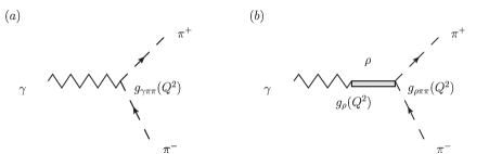
Figure 1: Diagrams relevant to the pion EM form factor $F_{V}^{\pi^{\pm}}$ in the general HLS Lagrangian (59).

Let us now evaluate the form (107) in the SS model. By using Eqs.(64), (73), (74), (76), with Eqs.(62) and (63), $\tilde{a}$ and $\tilde{z}$ are determined in the SS model as

$$\tilde{a}_{{}_{\rm SS}} = \frac{\pi}{4}\lambda_{1}\frac{\langle\psi_{1}\rangle\langle\psi_{1}(1-\psi_{0}^{2})\rangle}{\langle\psi_{1}^{2}\rangle}\simeq 2.62\,,$$ (113)

$$\tilde{z}_{{}_{\rm SS}} = \frac{\pi}{8}\lambda_{1}\left(\frac{\langle\psi_{1}\rangle\langle\psi_{1}(1-\psi_{0}^{2})\rangle}{\langle\psi_{1}^{2}\rangle}-\langle 1-\psi_{0}^{2}\rangle\right)=\frac{\tilde{a}}{2}-\frac{\pi}{8}\lambda_{1}\langle 1-\psi_{0}^{2}\rangle\simeq 0.08\,,$$ (114)

where we have used $\lambda_{1}\simeq 0.669$ in Eq.(63). Substituting the values in Eqs.(113) and (114) into Eq.(107), we evaluate the momentum-dependence of $F_{V}^{\pi^{\pm}}$ as a definite prediction of the SS model for the pion EM form factor. See Fig. 2 (black solid curve). Here we used the experimental input of $m_{\rho}$, $m_{\rho}=775$ MeV Amsler:2008zz . (We do not need an experimental input of $F_{\pi}$ for this quantity.) The experimental data from Refs. Amendolia:1986wj ; Volmer:2000ek ; Tadevosyan:2007yd ; Horn:2006tm are also shown. The $\chi^{2}$-fit results in good agreement with the data ($\chi^{2}/{\rm d.o.f}=147/53=2.8$).

For comparison, we have also shown the best fit curve (denoted by a red dotted line) resulted from fitting the parameters $(\tilde{a},\tilde{z})$ in the general HLS model (107) to the experimental data, which yields the best fit values of ${\tilde{a}}$ and $\tilde{z}$, ${\tilde{a}}|_{\rm best}=2.44$, $\tilde{z}|_{\rm best}=0.08$ ($\chi^{2}/{\rm d.o.f}=81/51=1.6$). It is interesting to note that the best fit values of $\tilde{a}$ and $\tilde{z}$ are quite close to those in the predicted curve, which reflects that the predicted curve fits well the experimental data. Comparison with the $\rho$ meson dominance with ${\tilde{a}}=2$ and ${\tilde{z}}=0$ in Eq,(107) is also shown by a blue dashed curve ($\chi^{2}/{\rm d.o.f}=226/53=4.3$).

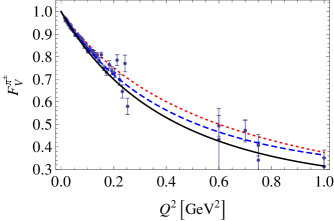
Figure 2: The prediction (black solid curve) of the pion EM form factor $F_{V}^{\pi^{\pm}}$ fitting the experimental data Amendolia:1986wj ; Volmer:2000ek ; Tadevosyan:2007yd ; Horn:2006tm with $\chi^{2}/{\rm d.o.f}=147/53=2.8$. The red dotted curve corresponds to the form factor in the $\rho$ meson dominance hypothesis with ${\tilde{a}}=2$ and ${\tilde{z}}=0$. ($\chi^{2}/{\rm d.o.f}=226/53=4.3$). The blue dashed curve is the best fit to experimental data with ${\tilde{a}}|_{\rm best}=2.44$, $\tilde{z}|_{\rm best}=0.08$ ($\chi^{2}/{\rm d.o.f}=81/51=1.6$).

Given any holographic model, our method can make a definite prediction of the model for the pion EM form factor in terms of two parameters $\tilde{a}$ and $\tilde{z}$ of the general HLS model which are determined by integrating out higher KK modes of the HLS gauge bosons. The best fit values in the above are the reference values to be compared with those of the holographic models. In comparison with the $\rho$ meson dominance, the deviation from ${\tilde{a}}=2$ and ${\tilde{z}}=0$ represents the contributions of higher KK modes in the generic holographic model as will be shown below.

We shall next discuss an implication of our method from a different point of view. We start with the expression of the form factor originally studied in the SS model, which takes the form of the infinite sum of KK modes of the HLS gauge fields:

$$F_{V}^{\pi^{\pm}}(Q^{2})\Bigg{|}_{\rm SS}=\sum_{k=1}^{\infty}\frac{g_{\rho_{k}}g_{\rho_{k}\pi\pi}}{m_{\rho_{k}}^{2}+Q^{2}}\,.$$ (115)

Our method is to integrate out the higher KK mode effects into the ${\cal O}(p^{4})$ terms of the HLS Lagrangian having only the $\rho$ meson as a dynamical degree of freedom. To be consistent with our method, we expand this form factor as

$$F_{V}^{\pi^{\pm}}(Q^{2})\Bigg{|}_{\rm SS} = \frac{g_{\rho}g_{\rho\pi\pi}}{m_{\rho}^{2}+Q^{2}}+\sum_{k=2}^{\infty}\frac{g_{\rho_{k}}g_{\rho_{k}\pi\pi}}{m_{\rho_{k}}^{2}+Q^{2}}\,$$ (116)

$$= \frac{g_{\rho}g_{\rho\pi\pi}}{m_{\rho}^{2}+Q^{2}}+\left(\sum_{k=2}^{\infty}\frac{g_{\rho_{k}}g_{\rho_{k}\pi\pi}}{m_{\rho_{k}}^{2}}\right)+\left(-\sum_{k=2}^{\infty}\frac{g_{\rho_{k}}g_{\rho_{k}\pi\pi}}{m_{\rho_{k}}^{2}}\frac{Q^{2}}{m_{\rho_{k}}^{2}}\right)\,,$$

up to ${\cal O}(Q^{4}/m_{\rho_{k}}^{4})$ ($k\geq 2$). Note that the ${\cal O}(p^{4})$ terms of the Lagrangian correspond to ${\cal O}(Q^{2})$ terms in the expansion of the pion EM form factor. Using the sum rules Sakai:2005yt ,

$$\sum_{k=1}^{\infty}\frac{g_{\rho_{k}}g_{\rho_{k}\pi\pi}}{m_{\rho_{k}}^{2}} = 1\,,$$ (117)

$$\sum_{k=1}^{\infty}\frac{g_{\rho_{k}}g_{\rho_{k}\pi\pi}}{m_{\rho_{k}}^{4}} = \frac{\pi}{8m_{\rho}^{2}}\lambda_{1}\langle 1-\psi_{0}^{2}\rangle\,,$$ (118)

we have

$$\sum_{k=2}^{\infty}\frac{g_{\rho_{k}}g_{\rho_{k}\pi\pi}}{m_{\rho_{k}}^{2}} = 1-\frac{g_{\rho}g_{\rho\pi\pi}}{m_{\rho}^{2}}\,,$$ (119)

$$-\sum_{k=2}^{\infty}\frac{g_{\rho_{k}}g_{\rho_{k}\pi\pi}}{m_{\rho_{k}}^{4}} = \frac{g_{\rho}g_{\rho\pi\pi}}{m_{\rho}^{4}}-\frac{\pi}{8m_{\rho}^{2}}\lambda_{1}\langle 1-\psi_{0}^{2}\rangle\,.$$ (120)

From Ref. Sakai:2005yt , we read off $g_{\rho}$ and $g_{\rho\pi\pi}$ as well as $m_{\rho}$ 

$$m_{\rho}^{2} = \lambda_{1}M_{KK}^{2}\,,$$ (121)

$$g_{\rho} = \sqrt{N_{c}G}\lambda_{1}M_{KK}^{2}\sqrt{\frac{\langle\psi_{1}\rangle^{2}}{\langle\psi_{1}^{2}\rangle}}\,,$$ (122)

$$g_{\rho\pi\pi} = \frac{\pi}{8}\frac{\lambda_{1}}{\sqrt{N_{c}G}}\sqrt{\frac{\langle\psi_{1}(1-\psi_{0}^{2})\rangle^{2}}{\langle\psi_{1}^{2}\rangle}}\,,$$ (123)

where we retained $\langle\psi_{1}^{2}\rangle$ to make explicit the ambiguity of the normalization of $\psi_{1}$ in contrast to Ref. Sakai:2005yt where the normalization of $\psi_{1}$ is fixed as $N_{c}G\langle\psi_{1}^{2}\rangle=1$. Substituting these into the right hand sides of Eqs.(119) and (120), we find

$$\sum_{k=2}^{\infty}\frac{g_{\rho_{k}}g_{\rho_{k}\pi\pi}}{m_{\rho_{k}}^{2}} = 1-\frac{\pi}{8}\lambda_{1}\frac{\langle\psi_{1}\rangle\langle\psi_{1}(1-\psi_{0}^{2})\rangle}{\langle\psi_{1}^{2}\rangle}\,,$$

$$-\sum_{k=2}^{\infty}\frac{g_{\rho_{k}}g_{\rho_{k}\pi\pi}}{m_{\rho_{k}}^{4}} = \frac{\pi}{8m_{\rho}^{2}}\lambda_{1}\left(\frac{\langle\psi_{1}\rangle\langle\psi_{1}(1-\psi_{0}^{2})\rangle}{\langle\psi_{1}^{2}\rangle}-\langle 1-\psi_{0}^{2}\rangle\right)\,.$$ (124)

Comparing Eqs.(113) and (114), we arrive at

$$\sum_{k=2}^{\infty}\frac{g_{\rho_{k}}g_{\rho_{k}\pi\pi}}{m_{\rho_{k}}^{2}} = 1-\frac{\tilde{a}_{{}_{\rm SS}}}{2}\,,$$

$$-\sum_{k=2}^{\infty}\frac{g_{\rho_{k}}g_{\rho_{k}\pi\pi}}{m_{\rho_{k}}^{4}} = \frac{{\tilde{z}}_{{}_{\rm SS}}}{m_{\rho}^{2}}\,.$$ (125)

and hence at the same result as that obtained by our method integrating out higher KK modes (Eq.(110) with Eqs.(113) and (114)):

$$F_{V}^{\pi^{\pm}}(Q^{2})|_{\rm SS}=\left(1-\frac{1}{2}\tilde{a}_{{}_{\rm SS}}\right)+\tilde{z}_{{}_{\rm SS}}\frac{Q^{2}}{m_{\rho}^{2}}+\frac{{\tilde{a}}_{{}_{\rm SS}}}{2}\frac{m_{\rho}^{2}}{m_{\rho}^{2}+Q^{2}}\,.$$ (126)

The deviation from the $\rho$ meson dominance is parameterized as

$$\Delta\tilde{a} \equiv \left(\frac{\tilde{a}-2}{2}\right)\,,$$ (127)

$$\Delta\tilde{z} \equiv (\tilde{z}-0)\,.$$ (128)

From Eq.(125) and referring to Ref. Sakai:2005yt , we may numerically read off these quantities in the SS model as

$$\Delta\tilde{a}_{{}_{\rm SS}} = \frac{{\tilde{a}}_{{}_{\rm SS}}}{2}-1\simeq 0.31\,,$$ (129)

$$= -\sum_{k=2}^{\infty}\frac{g_{\rho_{k}}g_{\rho_{k}\pi\pi}}{m_{\rho_{k}}^{2}}=(0.346)_{\rho^{\prime}}+(-0.0505)_{\rho^{\prime\prime}}+(0.0128)_{\rho^{\prime\prime\prime}}+\cdots\,,$$

$$\Delta\tilde{z}_{{}_{\rm SS}} = -m_{\rho}^{2}\sum_{k=2}^{\infty}\frac{g_{\rho_{k}}g_{\rho_{k}\pi\pi}}{m_{\rho_{k}}^{4}}=(0.0806)_{\rho^{\prime}}+(-0.0051)_{\rho^{\prime\prime}}+(0.0007)_{\rho^{\prime\prime\prime}}+\cdots\,.$$ (130)

This implies that the deviation from the $\rho$ meson dominance (${\tilde{a}}\simeq 2.62,{\tilde{z}}\simeq 0.08$) comes dominantly from the $\rho^{\prime}$-meson contribution.

Since the result is identical to that of our method which is manifestly EM-gauge invariant by construction (See Eqs.(36),(37) and (41)), the resultant form factor (126) should be EM gauge invariant. In fact, we have

$$F_{V}^{\pi^{\pm}}(0)|_{\rm SS}=\left(1-\frac{\tilde{a}_{{}_{\rm SS}}}{2}\right)+\frac{\tilde{a}_{{}_{\rm SS}}}{2}=1\,.$$ (131)

In contrast, a naive truncation corresponding to the Lagrangian in Eq.(33) would read

$$F_{V}^{\pi^{\pm}}(Q^{2})\Bigg{|}_{\rm SS}^{\rm trun}=\frac{g_{\rho}g_{\rho\pi\pi}}{m_{\rho}^{2}+Q^{2}}\,,$$ (132)

which corresponds to ignoring the last two terms in Eq.(116) coming from higher KK modes to both ${\cal O}(p^{2})$ and ${\cal O}(p^{4})$ terms. Since the Lagrangian (33) is gauge non-invariant, so is the form factor above,

$$F_{V}^{\pi^{\pm}}(0)\Bigg{|}_{\rm SS}^{\rm trun}=\frac{g_{\rho}g_{\rho\pi\pi}}{m_{\rho}^{2}}=\frac{\tilde{a}_{{}_{\rm SS}}}{2}\simeq 1.31\neq 1\,,$$ (133)

where we used Eq.(113) together with Eqs. (121), (122) and (123). Note that the truncation (132) is different from the $\rho$ meson dominance (111) which is gauge invariant.

IV.2 Anomaly-related intrinsic parity-odd processes

In this subsection we calculate momentum dependence of the IP-odd form factors, $\pi^{0}$-$\gamma$ and $\omega$-$\pi^{0}$ transition form factors. We also study several IP-odd vertex functions such as $\pi^{0}$-$\gamma^{*}$-$\gamma^{*}$ (Sec. IV.2.1), $\omega$-$\pi^{0}$-$\gamma^{*}$ (Sec. IV.2.2), $\gamma^{*}$-$\pi^{0}$-$\pi^{+}$-$\pi^{-}$ (Sec. IV.2.3), and $\omega\to\pi^{0}\pi^{+}\pi^{-}$ decay (Sec. IV.2.4), and discuss the $\rho/\omega$ meson dominance. Discussion of an alternative method, which leads to the same results as ours shown in this subsection as done in Sec. IV.1 (See Eq.(116)), will be given in Appendix C.

The IP-odd interactions in the general HLS model are read off from Eq.(81) together with the WZW term as  Harada:2003jx

$${\cal L}_{VV\pi} = -\frac{g^{2}N_{c}}{4\pi^{2}F_{\pi}}c_{3}\epsilon^{\mu\nu\lambda\sigma}{\rm tr}[\partial_{\mu}\rho_{\nu}\partial_{\lambda}\rho_{\sigma}\pi]\,,$$

$${\cal L}_{VA\pi} = -\frac{egN_{c}}{8\pi^{2}F\pi}(c_{4}-c_{3})\epsilon^{\mu\nu\lambda\sigma}{\rm tr}[\{\partial_{\mu}\rho_{\nu},\partial_{\lambda}A_{\sigma}\}\pi]\,,$$

$${\cal L}_{AA\pi} = -\frac{e^{2}N_{c}}{4\pi^{2}F\pi}(1-c_{4})\epsilon^{\mu\nu\lambda\sigma}{\rm tr}[\partial_{\mu}A_{\nu}\partial_{\lambda}A_{\sigma}\pi]\,,$$

$${\cal L}_{A\pi^{3}} = -i\frac{eN_{c}}{3\pi^{2}F_{\pi}^{3}}\left(1-\frac{3(c_{1}-c_{2}+c_{3})}{4}\right)\epsilon^{\mu\nu\lambda\sigma}{\rm tr}[A_{\mu}\partial_{\nu}\pi\partial_{\lambda}\pi\partial_{\sigma}\pi]\,,$$

$${\cal L}_{V\pi^{3}} = -i\frac{gN_{c}}{4\pi^{2}F_{\pi}^{3}}(c_{1}-c_{2}-c_{3})\epsilon^{\mu\nu\lambda\sigma}{\rm tr}[\rho_{\mu}\partial_{\nu}\pi\partial_{\lambda}\pi\partial_{\sigma}\pi]\,.$$ (134)

For relevant Feynman graphs for each IP-odd process, see Figs.4, 5, 6, and 7 in Ref. Harada:2003jx .

IV.2.1 $\pi^{0}$-$\gamma^{*}$-$\gamma^{*}$ vertex function and $\pi^{0}$-$\gamma$ transition form factor

We start with an expression of effective $\pi^{0}$-$\gamma^{*}$-$\gamma^{*}$ vertex function from the general HLS Lagrangian (Eqs.(59) and (134)):

$$\Gamma^{\mu\nu}[\pi^{0},\gamma^{*}_{\mu}(q_{1}),\gamma_{\nu}^{*}(q_{2})] = \frac{e^{2}N_{c}}{12\pi^{2}F_{\pi}}\epsilon^{\mu\nu\alpha\beta}q_{1\alpha}q_{2\beta}\cdot\Bigg{[}(1-c_{4})+\frac{(c_{4}-c_{3})}{4}\times$$

$$\left\{D_{\rho}(q_{1}^{2})\left(1-g^{2}z_{3}\frac{q_{1}^{2}}{m_{\rho}^{2}}\right)+D_{\omega}(q_{1}^{2})\left(1-g^{2}z_{3}\frac{q_{1}^{2}}{m_{\omega}^{2}}\right)+(q_{1}^{2}\to q_{2}^{2})\right\}$$

$$+\frac{c_{3}}{2}\left\{D_{\rho}(q_{1}^{2})\left(1-g^{2}z_{3}\frac{q_{1}^{2}}{m_{\rho}^{2}}\right)\cdot D_{\omega}(q_{2}^{2})\left(1-g^{2}z_{3}\frac{q_{2}^{2}}{m_{\omega}^{2}}\right)+(q_{1}^{2}\leftrightarrow q_{2}^{2})\right\}\Bigg{]}\,,$$

where $q_{1,2}$ represent outgoing four-momenta of virtual photons $\gamma^{*}$ and

$$D_{\rho,\omega}(p^{2}) \equiv \frac{m_{\rho,\omega}^{2}}{m_{\rho,\omega}^{2}-p^{2}}\,,$$ (136)

$$g_{\rho,\omega}(p^{2}) \equiv \frac{m_{\rho,\omega}^{2}}{g}\left(1-g^{2}z_{3}\frac{p^{2}}{m_{\rho,\omega}^{2}}\right)\,.$$ (137)

We further rewrite Eq.(LABEL:pi2g:form1) as follows:

$$\Gamma^{\mu\nu}[\pi^{0},\gamma^{*}_{\mu}(q_{1}),\gamma_{\nu}^{*}(q_{2})] = \frac{e^{2}N_{c}}{12\pi^{2}F_{\pi}}\epsilon^{\mu\nu\alpha\beta}q_{1\alpha}q_{2\beta}\Bigg{[}A^{\pi 2\gamma}+\frac{B^{\pi 2\gamma}}{4}\left\{D_{\rho}(q_{1}^{2})+D_{\omega}(q_{1}^{2})+(q_{1}^{2}\to q_{2}^{2})\right\}$$ (138)

$$+\frac{C^{\pi 2\gamma}}{2}\left\{D_{\rho}(q_{1}^{2})\cdot D_{\omega}(q_{2}^{2})+(q_{1}^{2}\leftrightarrow q_{2}^{2})\right\}\Bigg{]}\,,$$

where we have used an identity for an arbitrary coefficient $C$,

$$D_{\rho,\omega}(p^{2})\left(1-C\cdot\frac{p^{2}}{m_{\rho,\omega}^{2}}\right)=(1-C)D_{\rho,\omega}(p^{2})+C\,,$$ (139)

and defined

$$A^{\pi 2\gamma} = 1-(1-g^{2}z_{3})(c_{4}+c_{3}\cdot g^{2}z_{3})\,,$$ (140)

$$B^{\pi 2\gamma} = (1-g^{2}z_{3})\left[(c_{4}+c_{3}\cdot g^{2}z_{3})-c_{3}(1-g^{2}z_{3})\right]\,,$$ (141)

$$C^{\pi 2\gamma} = c_{3}(1-g^{2}z_{3})^{2}\,.$$ (142)

Note that these parameters satisfy

$$A^{\pi 2\gamma}+B^{\pi 2\gamma}+C^{\pi 2\gamma}=1$$ (143)

which reproduces the low-energy theorem:

$$\Gamma^{\mu\nu}[\pi^{0},\gamma^{*}_{\mu}(q_{1}),\gamma_{\nu}^{*}(q_{2})]\stackrel{{\scriptstyle{q_{1}^{2},q_{2}^{2}\to 0}}}{{\longrightarrow}}\frac{e^{2}N_{c}}{12\pi^{2}F_{\pi}}\epsilon^{\mu\nu\alpha\beta}q_{1\alpha}q_{2\beta}\,.$$ (144)

The $\rho/\omega$ meson dominance GellMann:1962jt for this process is defined in a way similar to Eq.(111) by taking $A^{\pi 2\gamma}=B^{\pi 2\gamma}=0$ ($C^{\pi 2\gamma}=1$)

$$\Gamma^{\mu\nu}[\pi^{0},\gamma^{*}_{\mu}(q_{1}),\gamma_{\nu}^{*}(q_{2})]=\frac{e^{2}N_{c}}{24\pi^{2}F_{\pi}}\epsilon^{\mu\nu\alpha\beta}q_{1\alpha}q_{2\beta}\left(D_{\rho}(q_{1}^{2})\cdot D_{\omega}(q_{2}^{2})+(q_{1}^{2}\leftrightarrow q_{2}^{2})\right)\,.$$ (145)

The $\pi^{0}$-$\gamma$ transition form factor $F_{\pi^{0}\gamma}$ is obtained from Eq.(138) by setting one of the photon-momentum squared ($q_{1}^{2}$ or $q_{2}^{2}$) to be zero:

$$F_{\pi^{0}\gamma}(Q^{2})=\left(1-{\tilde{c}}\right)+\frac{{\tilde{c}}}{2}[D_{\rho}(Q^{2})+D_{\omega}(Q^{2})]\,,$$ (146)

where $Q^{2}=-q_{1}^{2}$ (or $-q_{2}^{2}$) and we defined

$${\tilde{c}}\equiv 1-(A^{\pi 2\gamma}+B^{\pi 2\gamma})\,.$$ (147)

The $\rho/\omega$ meson dominance defined by Eq.(145) reads

$$F_{\pi^{0}\gamma}(Q^{2}) = \frac{1}{2}\left(\frac{m_{\rho}^{2}}{m_{\rho}^{2}+Q^{2}}+\frac{m_{\omega}^{2}}{m_{\omega}^{2}+Q^{2}}\right)\,,$$

$${\tilde{c}} = 1\,.$$ (148)

We shall now evaluate the parameters in Eqs.(138) and (146) in the SS model. Using Eqs.(64), (73), (85), and (86), we calculate $A^{\pi 2\gamma}$, $B^{\pi 2\gamma}$, and $C^{\pi 2\gamma}$ to get

$$A^{\pi 2\gamma}_{{}_{\rm SS}} = 1-\left[\frac{\langle\psi_{1}\rangle\langle\langle\dot{\psi}_{0}\psi_{1}\rangle\rangle}{\langle\psi_{1}^{2}\rangle}-\frac{1}{2}\frac{\langle\psi_{1}\rangle^{2}\langle\langle\dot{\psi}_{0}\psi_{1}^{2}\rangle\rangle}{\langle\psi_{1}^{2}\rangle^{2}}\right]\simeq 1-(0.61)=0.39\,,$$ (149)

$$B^{\pi 2\gamma}_{{}_{\rm SS}} = \frac{\langle\psi_{1}\rangle\langle\langle\dot{\psi}_{0}\psi_{1}\rangle\rangle}{\langle\psi_{1}^{2}\rangle}-\frac{\langle\psi_{1}\rangle^{2}\langle\langle\dot{\psi}_{0}\psi_{1}^{2}\rangle\rangle}{\langle\psi_{1}^{2}\rangle^{2}}\simeq-0.09\,,$$ (150)

$$C^{\pi 2\gamma}_{{}_{\rm SS}} = \frac{1}{2}\left[\frac{\langle\psi_{1}\rangle^{2}\langle\langle\dot{\psi}_{0}\psi_{1}^{2}\rangle\rangle}{\langle\psi_{1}^{2}\rangle^{2}}\right]\simeq 0.50\,.$$ (151)

By using these values and Eq.(147), the value of ${\tilde{c}}$ of the SS model is calculated as

$${\tilde{c}}_{{}_{\rm SS}}\simeq 1.31\,,$$ (152)

which implies that the form factor $F_{\pi^{0}\gamma}$ in the SS model violates (about 30%) the $\rho/\omega$ meson dominance. Putting the value in Eq.(152) into Eq.(146), we evaluate momentum dependence of $F_{\pi^{0}\gamma}$ as a definite prediction of the SS model for the $\pi^{0}$-$\gamma$ transition form factor. See Fig. 3 (black solid curve). Here use has been made of the experimental inputs of $m_{\rho}$ and $m_{\omega}$, $m_{\rho}=775$ MeV and $m_{\omega}=783$ MeV Amsler:2008zz . The experimental data are from Ref. Behrend:1990sr which is the only experiment in the space-like region . Figure 3 shows that the momentum dependence of $F_{\pi^{0}\gamma}$ in the SS model disagrees with the experiment ($\chi^{2}/{\rm d.o.f}=63/5=13$).

For a comparison, in Fig. 3 we plot a curve drawn by a blue dashed line obtained by fitting the parameter $\tilde{c}$ of the general HLS model to the experimental data, which yields the best fit value of $\tilde{c}$, $\tilde{c}|_{\rm best}=1.03$ ($\chi^{2}/{\rm d.o.f}=3/4=0.7$). This best fit value is very close to ${\tilde{c}}=1$ of the $\rho/\omega$ meson dominance (red dotted curve in the figure).

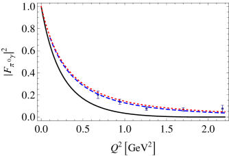
Figure 3: The prediction (black solid curve) of the $\pi^{0}$-$\gamma$ transition form factor $F_{\pi^{0}\gamma}$ with respect to space-like momentum-squared $Q^{2}$. Comparison with the experimental data Behrend:1990sr yields $\chi^{2}/{\rm d.o.f}=63/5=13$. The blue dashed and red dotted curves respectively correspond to the best fit curve with ${\tilde{c}}_{\rm best}=1.03$ ($\chi^{2}/{\rm d.o.f}=3.0/4=0.7$) and the $\rho/\omega$ meson dominance with ${\tilde{c}}=1$ ($\chi^{2}/{\rm d.o.f}=4.8/5=1.0$).

IV.2.2 $\omega$-$\pi^{0}$-$\gamma^{*}$ vertex function and $\omega$-$\pi^{0}$ transition form factor

We begin with an expression of effective $\omega$-$\pi^{0}$-$\gamma^{*}$ vertex function obtained from the general HLS Lagrangian (Eqs.(59) and (134)):

$$\Gamma^{\mu\nu}[\omega_{\mu}(p),\pi^{0},\gamma^{*}_{\nu}(k)] = \frac{eN_{c}}{8\pi^{2}F_{\pi}}\epsilon^{\mu\nu\alpha\beta}p_{\alpha}k_{\beta}\cdot g\left[\left(\frac{c_{4}-c_{3}}{2}\right)+c_{3}\cdot D_{\rho}(k^{2})\left(1-g^{2}z_{3}\frac{k^{2}}{m_{\rho}^{2}}\right)\right]\,,$$ (153)

where $p$ and $k$ respectively denote incoming four-momentum of $\omega$ and outgoing momentum of $\gamma^{*}$. Using the identity (139), we rewrite Eq.(153) into the following form:

$$\Gamma^{\mu\nu}[\omega_{\mu}(p),\pi^{0},\gamma^{*}_{\nu}(k)] = \frac{eN_{c}}{8\pi^{2}F_{\pi}}\epsilon^{\mu\nu\alpha\beta}p_{\alpha}k_{\beta}\cdot\left[A^{\omega\pi\gamma}+B^{\omega\pi\gamma}D_{\rho}(k^{2})\right]\,,$$ (154)

where

$$A^{\omega\pi\gamma} = \frac{1}{2}g\left[(c_{4}+c_{3}\cdot g^{2}z_{3})-c_{3}(1-g^{2}z_{3})\right]\,,$$ (155)

$$B^{\omega\pi\gamma} = gc_{3}(1-g^{2}z_{3})\,.$$ (156)

Note that $(A^{\omega\pi\gamma}+B^{\omega\pi\gamma})$ is not constrained, which is consistent with the fact that there is no low-energy theorem for Eq.(154) in the low-energy limit:

$$\Gamma^{\mu\nu}[\omega_{\mu}(p),\pi^{0},\gamma^{*}_{\nu}(k)] \stackrel{{\scriptstyle k^{2}\to 0}}{{\longrightarrow}} \frac{eN_{c}}{8\pi^{2}F_{\pi}}\epsilon^{\mu\nu\alpha\beta}p_{\alpha}k_{\beta}\cdot\left[A^{\omega\pi\gamma}+B^{\omega\pi\gamma}\right]\,,$$ (157)

in contrast to Eq.(143) for the $\pi^{0}$-$\gamma^{*}$-$\gamma^{*}$ vertex function.

The $\omega$-$\pi^{0}$ transition form factor $F_{\omega\pi^{0}}$ can be extracted from the $\omega\to\pi^{0}l^{+}l^{-}$ decay width $\Gamma(\omega\to\pi^{0}l^{+}l^{-})$ ($l^{\pm}=e^{\pm},\mu^{\pm}$) which is calculated through the effective $\omega$-$\pi^{0}$-$\gamma^{*}$ vertex function as

$$\Gamma(\omega\to\pi^{0}l^{+}l^{-}) = \int^{(m_{\omega}-m_{\pi^{0}})^{2}}_{4m_{l}^{2}}dq^{2}\frac{\alpha}{3\pi}\frac{\Gamma(\omega\to\pi^{0}\gamma)}{q^{2}}\left(1+\frac{2m_{l}^{2}}{q^{2}}\right)\sqrt{\frac{q^{2}-4m_{l}^{2}}{q^{2}}}$$ (158)

$$\times\left[\left(1+\frac{q^{2}}{m_{\omega}^{2}-m_{\pi^{0}}^{2}}\right)^{2}-\frac{4m_{\omega}^{2}q^{2}}{(m_{\omega}^{2}-m_{\pi^{0}}^{2})^{2}}\right]^{3/2}\cdot|F_{\omega\pi^{0}}(q^{2})|^{2}\,,$$

where $\Gamma(\omega\to\pi^{0}\gamma)$ denotes the $\omega\to\pi^{0}\gamma$ decay width ,

$$\Gamma(\omega\to\pi^{0}\gamma)=\frac{3\alpha}{64\pi^{4}F_{\pi}^{2}}\,\,g_{\omega\pi\gamma}^{2}\,\left(\frac{m_{\omega}^{2}-m_{\pi^{0}}^{2}}{2m_{\omega}}\right)^{3}\,,$$ (159)

with

$$g_{\omega\pi\gamma}=A^{\omega\pi\gamma}+B^{\omega\pi\gamma}=\frac{g(c_{3}+c_{4})}{2}\,.$$ (160)

The transition form factor $F_{\omega\pi^{0}}$ is then expressed as

$$F_{\omega\pi^{0}}(q^{2})=(1-\tilde{r})+\tilde{r}D_{\rho}(q^{2})\,,$$ (161)

where

$$\tilde{r}=\frac{B^{\omega\pi\gamma}}{A^{\omega\pi\gamma}+B^{\omega\pi\gamma}}\,.$$ (162)

The $\rho$ meson dominance GellMann:1962jt for this transition form factor is defined in a way similar to Eq.(111) by taking $\tilde{r}=1$ as

$$F_{\omega\pi^{0}}(q^{2}) = \frac{m_{\rho}^{2}}{m_{\rho}^{2}-q^{2}}\,,$$

$$\tilde{r} = 1\,.$$ (163)

Let us now evaluate the parameter ${\tilde{r}}$ in Eq.(161) in the SS model. Using Eqs.(64), (73), (85), and (86), we have

$$A_{{}_{\rm SS}}^{\omega\pi\gamma} = -\frac{1}{2\sqrt{N_{c}G}}\left[\frac{\langle\langle\dot{\psi}_{0}\psi_{1}\rangle\rangle}{\sqrt{\langle\psi_{1}^{2}\rangle}}-\frac{\langle\psi_{1}\rangle\langle\langle\dot{\psi}_{0}\psi_{1}^{2}\rangle\rangle}{\langle\psi_{1}^{2}\rangle^{3/2}}\right]\,,$$ (164)

$$B_{{}_{\rm SS}}^{\omega\pi\gamma} = -\frac{1}{2\sqrt{N_{c}G}}\left[\frac{\langle\psi_{1}\rangle\langle\langle\dot{\psi}_{0}\psi_{1}^{2}\rangle\rangle}{\langle\psi_{1}^{2}\rangle^{3/2}}\right]\,,$$ (165)

and calculate $\tilde{r}$ to get

$${\tilde{r}}_{{}_{\rm SS}}\simeq 1.53\,,$$ (166)

which implies that the form factor $F_{\omega\pi^{0}}$ in the SS model violates (about 50%) the $\rho$ meson dominance with ${\tilde{r}}=1$. The predicted curve in time-like momentum region is shown in Fig. 4 as a black solid line together with the experimental data Akhmetshin:2005vy ; :2009wb . Figure. 4 shows that the momentum dependence of $F_{\omega\pi^{0}}$ in the SS model is consistent with the experimental data ($\chi^{2}/{\rm d.o.f}=45/31=1.5$).

The predicted curve is compared with a blue dashed curve obtained by fitting the parameter $\tilde{r}$ of the general HLS model to the experimental data, which gives the best fit value of ${\tilde{r}}$, ${\tilde{r}}_{\rm best}=2.08$ ($\chi^{2}/{\rm d.o.f}=24/30=0.8$). Comparison with the $\rho$ meson dominance with ${\tilde{r}}=1$ (red dotted curve) is also given ($\chi^{2}/{\rm d.o.f}=124/31=4.0$).

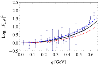
Figure 4: The prediction (black solid curve) of the $\omega$-$\pi^{0}$ transition form factor $F_{\omega\pi^{0}}(q^{2})$ with respect to time-like momentum $q$. Comparison with the experimental data Akhmetshin:2005vy ; :2009wb yields $\chi^{2}/{\rm d.o.f}=45/31=1.5$. The best fit curve with ${\tilde{r}}_{\rm best}=2.08$ ($\chi^{2}/{\rm d.o.f}=24/30=0.8$) and curve corresponding to the $\rho$ meson dominance with ${\tilde{r}}=1$ ($\chi^{2}/{\rm d.o.f}=124/31=4.0$) are drawn by blue dashed and red dotted lines, respectively.

IV.2.3 $\gamma^{*}$-$\pi^{0}$-$\pi^{+}$-$\pi^{-}$ vertex function

We start with an expression of effective $\gamma^{*}$-$\pi^{0}$-$\pi^{+}$-$\pi^{-}$ vertex function obtained from the general HLS Lagrangian (Eqs.(59) and (134)):

$$\Gamma_{\mu}[\gamma^{*}_{\mu}(p),\pi^{0}(q_{0}),\pi^{+}(q_{+}),\pi^{-}(q_{-})]$$ (167)

$$= -\frac{eN_{c}}{12\pi^{2}F_{\pi}^{3}}\epsilon_{\mu\nu\alpha\beta}q_{0}^{\nu}q_{+}^{\alpha}q_{-}^{\beta}\Bigg{[}1-\frac{3}{4}(c_{1}-c_{2}+c_{4})+\frac{3}{4}(c_{1}-c_{2}-c_{3})D_{\omega}(p^{2})\left(1-g^{2}z_{3}\frac{p^{2}}{m_{\omega}^{2}}\right)$$

$$+\left\{\frac{c_{4}-c_{3}}{4}+\frac{c_{3}}{2}D_{\omega}(p^{2})\left(1-g^{2}z_{3}\frac{p^{2}}{m_{\omega}^{2}}\right)\right\}\times\Bigg{\{}D_{\rho}((q_{+}+q_{-})^{2})\left(1-\frac{1}{2}g^{2}z_{4}\frac{(q_{+}+q_{-})^{2}}{m_{\rho}^{2}}\right)$$

$$+D_{\rho}((q_{-}+q_{0})^{2})\left(1-\frac{1}{2}g^{2}z_{4}\frac{(q_{-}+q_{0})^{2}}{m_{\rho}^{2}}\right)+D_{\rho}((q_{0}+q_{+})^{2})\left(1-\frac{1}{2}g^{2}z_{4}\frac{(q_{0}+q_{+})^{2}}{m_{\rho}^{2}}\right)\Bigg{\}}\Bigg{]}\,,$$

where $p$ and $q_{\pm,0}$ respectively stand for incoming four-momentum of $\gamma^{*}$ and outgoing four-momenta of $\pi^{\pm}$ and $\pi^{0}$. By using the identity (139), the expression (167) may be rewritten as

$$\Gamma_{\mu}[\gamma^{*}_{\mu}(p),\pi^{0}(q_{0}),\pi^{+}(q_{+}),\pi^{-}(q_{-})]$$ (168)

$$= -\frac{eN_{c}}{12\pi^{2}F_{\pi}^{3}}\epsilon_{\mu\nu\alpha\beta}q_{0}^{\nu}q_{+}^{\alpha}q_{-}^{\beta}\Bigg{[}A^{\gamma 3\pi}+B^{\gamma 3\pi}\cdot D_{\omega}(p^{2})+\frac{C^{\gamma 3\pi}}{3}\cdot\Bigg{\{}D_{\rho}((q_{+}+q_{-})^{2})+D_{\rho}((q_{-}+q_{0})^{2})+D_{\rho}((q_{0}+q_{+})^{2})\Bigg{\}}$$

$$+\frac{D^{\gamma 3\pi}}{3}\cdot D_{\omega}(p^{2})\cdot\Bigg{\{}D_{\rho}((q_{+}+q_{-})^{2})+D_{\rho}((q_{-}+q_{0})^{2})+D_{\rho}((q_{0}+q_{+})^{2})\Bigg{\}}\Bigg{]}\,,$$

where

$$A^{\gamma 3\pi} = 1-\frac{3}{4}\Bigg{[}(1-g^{2}z_{3})(c_{1}-c_{2}+c_{3})-2c_{3}(1-g^{2}z_{3})\left(1-\frac{1}{2}g^{2}z_{4}\right)+\left(1-\frac{1}{2}g^{2}z_{4}\right)(c_{3}+c_{4})\Bigg{]}\,,$$ (169)

$$B^{\gamma 3\pi} = \frac{3}{4}\left[(1-g^{2}z_{3})(c_{1}-c_{2}+c_{3})-2c_{3}(1-g^{2}z_{3})\left(1-\frac{1}{2}g^{2}z_{4}\right)\right]\,,$$ (170)

$$C^{\gamma 3\pi} = \frac{3}{4}\left[-2c_{3}(1-g^{2}z_{3})\left(1-\frac{1}{2}g^{2}z_{4}\right)+\left(1-\frac{1}{2}g^{2}z_{4}\right)(c_{3}+c_{4})\right]\,,$$ (171)

$$D^{\gamma 3\pi} = \frac{3}{4}\left[2c_{3}(1-g^{2}z_{3})\left(1-\frac{1}{2}g^{2}z_{4}\right)\right]\,.$$ (172)

Note that these parameters satisfy

$$A^{\gamma 3\pi}+B^{\gamma 3\pi}+C^{\gamma 3\pi}+D^{\gamma 3\pi}=1$$ (173)

which reproduces the low-energy theorem:

$$\Gamma_{\mu}[\gamma^{*}_{\mu}(p),\pi^{0}(q_{0}),\pi^{+}(q_{+}),\pi^{-}(q_{-})]\stackrel{{\scriptstyle q_{\pm,0}^{2}\to 0}}{{\longrightarrow}}-\frac{eN_{c}}{12\pi^{2}F_{\pi}^{3}}\epsilon_{\mu\nu\alpha\beta}q_{0}^{\nu}q_{+}^{\alpha}q_{-}^{\beta}\,.$$ (174)

The $\rho/\omega$ meson dominance for this process is defined in a way similar to Eq.(111) by taking $A^{\gamma 3\pi}=B^{\gamma 3\pi}=C^{\gamma 3\pi}=0$ ($D^{\gamma 3\pi}=1$) as

$$\Gamma_{\mu}[\gamma^{*}_{\mu}(p),\pi^{0}(q_{0}),\pi^{+}(q_{+}),\pi^{-}(q_{-})]$$ (175)

$$= -\frac{eN_{c}}{36\pi^{2}F_{\pi}^{3}}\epsilon_{\mu\nu\alpha\beta}q_{0}^{\nu}q_{+}^{\alpha}q_{-}^{\beta}\,\frac{m_{\omega}^{2}}{m_{\omega}^{2}-p^{2}}\left(\frac{m_{\rho}^{2}}{m_{\rho}^{2}-(q_{+}+q_{-})^{2}}+(q_{+}\leftrightarrow q_{0})+(q_{-}\leftrightarrow q_{0})\right)\,.$$

We shall now evaluate the parameters in Eq.(168) in the SS model. Using Eqs.(64), (73), (74), and (83)-(86), we have

$$A_{{}_{\rm SS}}^{\gamma 3\pi} = 1-\frac{3}{4}\Bigg{[}\frac{\langle\psi_{1}\rangle\langle\langle\dot{\psi}_{0}\psi_{1}(1-\psi_{0}^{2})\rangle\rangle}{\langle\psi_{1}^{2}\rangle}+\frac{\langle\langle\dot{\psi}_{0}\psi_{1}\rangle\rangle\langle\psi_{1}(1-\psi_{0}^{2})\rangle}{\langle\psi_{1}^{2}\rangle}-\frac{\langle\langle\dot{\psi}_{0}\psi_{1}^{2}\rangle\rangle\langle\psi_{1}\rangle\langle\psi_{1}(1-\psi_{0}^{2})\rangle}{\langle\psi_{1}^{2}\rangle^{2}}\Bigg{]}\,,$$ (176)

$$B_{{}_{\rm SS}}^{\gamma 3\pi} = \frac{3}{4}\Bigg{[}\frac{\langle\psi_{1}\rangle\langle\langle\dot{\psi}_{0}\psi_{1}(1-\psi_{0}^{2})\rangle\rangle}{\langle\psi_{1}^{2}\rangle}-\frac{\langle\langle\dot{\psi}_{0}\psi_{1}^{2}\rangle\rangle\langle\psi_{1}\rangle\langle\psi_{1}(1-\psi_{0}^{2})\rangle}{\langle\psi_{1}^{2}\rangle^{2}}\Bigg{]}\,,$$ (177)

$$C_{{}_{\rm SS}}^{\gamma 3\pi} = \frac{3}{4}\Bigg{[}\frac{\langle\langle\dot{\psi}_{0}\psi_{1}\rangle\rangle\langle\psi_{1}(1-\psi_{0}^{2})\rangle}{\langle\psi_{1}^{2}\rangle}-\frac{\langle\langle\dot{\psi}_{0}\psi_{1}^{2}\rangle\rangle\langle\psi_{1}\rangle\langle\psi_{1}(1-\psi_{0}^{2})\rangle}{\langle\psi_{1}^{2}\rangle^{2}}\Bigg{]}\,,$$ (178)

$$D_{{}_{\rm SS}}^{\gamma 3\pi} = \frac{3}{4}\left[\frac{\langle\langle\dot{\psi}_{0}\psi_{1}^{2}\rangle\rangle\langle\psi_{1}\rangle\langle\psi_{1}(1-\psi_{0}^{2})\rangle}{\langle\psi_{1}^{2}\rangle^{2}}\right]\,.$$ (179)

They are calculated in the SS model as

$$A_{{}_{\rm SS}}^{\gamma 3\pi} \simeq 1-(1.03)=-0.03\,,$$

$$B_{{}_{\rm SS}}^{\gamma 3\pi} \simeq 0.04\,,$$

$$C_{{}_{\rm SS}}^{\gamma 3\pi} \simeq -0.51\,,$$

$$D_{{}_{\rm SS}}^{\gamma 3\pi} \simeq 1.50\,,$$ (180)

in which $D_{{}_{\rm SS}}^{\gamma 3\pi}\neq 1$ implies that the effective $\gamma^{*}$-$\pi^{0}$-$\pi^{+}$-$\pi^{-}$ vertex function in the SS model violates (about 50%) the $\rho/\omega$ meson dominance.

IV.2.4 $\omega\to\pi^{0}\pi^{+}\pi^{-}$ decay

The $\omega\to\pi^{0}\pi^{+}\pi^{-}$ decay width is given by

$$\Gamma(\omega\to\pi^{0}\pi^{+}\pi^{-})=\frac{m_{\omega}}{192\pi^{3}}\int\int dE_{+}dE_{-}\left(|\vec{q}_{+}|^{2}|\vec{q}_{-}|^{2}-(\vec{q}_{+}\cdot\vec{q}_{-})^{2}\right)|F_{\omega\to 3\pi}|^{2}\,,$$ (181)

where $E_{\pm}$ and $\vec{q}_{\pm}$ are respectively energies and three-momenta of $\pi^{\pm}$ in the rest frame of $\omega$. We construct the $\omega\to 3\pi$ form factor $F_{\omega\to 3\pi}$ from the general HLS Lagrangian (Eqs.(59) and (134)):

$$F_{\omega\to 3\pi} = -\frac{N_{c}}{4\pi^{2}F_{\pi}m_{\rho}^{2}}\Bigg{[}\frac{3ag}{4}g^{2}(c_{1}-c_{2}-c_{3})+\frac{ag^{3}}{2}c_{3}\Bigg{\{}\left(1-\frac{g^{2}z_{4}}{2}\frac{(q_{+}+q_{-})^{2}}{m_{\rho}^{2}}\right)\cdot D_{\rho}((q_{+}+q_{-})^{2})$$ (182)

$$+(q_{+}\leftrightarrow q_{0})+(q_{-}\leftrightarrow q_{0})\Bigg{\}}\Bigg{]}\,,$$

where $q_{0,\pm}$ are four-momenta of $\pi^{0,\pm}$, respectively. Using the identity in Eq.(139) we may rewrite $F_{\omega\to 3\pi}$ into the following form:

$$F_{\omega\to 3\pi}=-\frac{N_{c}}{4\pi^{2}F_{\pi}m_{\rho}^{2}}g_{\rho\pi\pi}\Bigg{[}A^{\omega 3\pi}+\frac{B^{\omega 3\pi}}{3}\Bigg{\{}D_{\rho}((q_{+}+q_{-})^{2})+(q_{+}\leftrightarrow q_{0})+(q_{-}\leftrightarrow q_{0})\Bigg{\}}\Bigg{]}\,,$$ (183)

where

$$A^{\omega 3\pi} = \frac{3}{2}\frac{g^{2}(c_{1}-c_{2}+c_{3})}{1-g^{2}z_{4}/2}-3g^{2}c_{3}\,,$$ (184)

$$B^{\omega 3\pi} = 3g^{2}c_{3}\,.$$ (185)

Note that $(A^{\omega 3\pi}+B^{\omega 3\pi})$ is not constrained because there is no low-energy theorem for Eq.(183) in the low-energy limit:

$$F_{\omega\to 3\pi}\stackrel{{\scriptstyle q^{2}_{\pm,0}\to 0}}{{\longrightarrow}}-\frac{N_{c}}{4\pi^{2}F_{\pi}m_{\rho}^{2}}g_{\rho\pi\pi}\left(A^{\omega 3\pi}+B^{\omega 3\pi}\right)\,,$$ (186)

in contrast to Eqs.(143) and (174) for the $\pi^{0}$-$\gamma^{*}$-$\gamma^{*}$ and $\gamma^{*}$-$\pi^{0}$-$\pi^{+}$-$\pi^{-}$ vertex functions, respectively. The $\rho$ meson dominance GellMann:1962jt for this process is defined in a way similar to Eq.(111) by taking $A^{\omega 3\pi}=0$ in the form factor $F_{\omega\to 3\pi}$ as

$$F_{\omega\to 3\pi}=-\frac{N_{c}}{12\pi^{2}F_{\pi}m_{\rho}^{2}}g_{\rho\pi\pi}\cdot B^{\omega 3\pi}\cdot\left[\frac{m_{\rho}^{2}}{m_{\rho}^{2}-(q_{+}+q_{-})^{2}}+(q_{+}\leftrightarrow q_{0})+(q_{-}\leftrightarrow q_{0})\right]\,.$$ (187)

We shall evaluate the parameters in Eq.(183) in the SS model. Using Eqs.(64), (74), (83), (84), and (85), we have

$$A_{{}_{\rm SS}}^{\omega 3\pi} = \frac{3}{2N_{c}G}\left(\frac{\langle\langle\psi_{1}\dot{\psi}_{0}(1-\psi_{0}^{2})\rangle\rangle}{\langle\psi_{1}(1-\psi_{0}^{2})\rangle}-\frac{\langle\langle\dot{\psi}_{0}\psi_{1}^{2}\rangle\rangle}{\langle\psi_{1}^{2}\rangle}\right)\,,$$ (188)

$$B_{{}_{\rm SS}}^{\omega 3\pi} = \frac{3}{2N_{c}G}\frac{\langle\langle\dot{\psi}_{0}\psi_{1}^{2}\rangle\rangle}{\langle\psi_{1}^{2}\rangle}\,,$$ (189)

which are calculated in the SS model as

$$A_{{}_{\rm SS}}^{\omega 3\pi} \simeq 2.31\,,$$

$$B_{{}_{\rm SS}}^{\omega 3\pi} \simeq 81.01\,,$$ (190)

where we used the experimental inputs of $m_{\rho}$ and $F_{\pi}$, $m_{\rho}=775$ MeV and $F_{\pi}=92.4$ MeV Amsler:2008zz , to determine the value of $(N_{c}G)$ ($N_{c}G\simeq 0.01$). An amount of deviation from the $\rho$ meson dominance is estimated independently of value of $(N_{c}G)$ as

$$\frac{B_{{}_{\rm SS}}^{\omega 3\pi}}{A_{{}_{\rm SS}}^{\omega 3\pi}+B_{{}_{\rm SS}}^{\omega 3\pi}}\simeq 0.97\,,$$ (191)

which implies that the form factor $F_{\omega\to 3\pi}$ in the SS model is well approximated by the $\rho$ meson dominance.

Let us now calculate the decay width $\Gamma(\omega\to\pi^{0}\pi^{+}\pi^{-})$ in the SS model. To do this, we first estimate the value of $g_{\rho\pi\pi}$ which appears in Eq.(183) as the overall coefficient. Using Eq.(C.278) and the experimental values of $m_{\rho}$ and $F_{\pi}$, we get $g_{\rho\pi\pi}|_{\rm SS}\simeq 4.84$. Second, we evaluate the phase space integral using experimental inputs for $m_{\pi^{\pm,0}}$ and $m_{\omega}$, $m_{\pi^{\pm}}=140$ MeV, $m_{\pi^{0}}=135$ MeV and $m_{\omega}=783$ MeV Amsler:2008zz . Thus we obtain

$$\Gamma(\omega\to\pi^{0}\pi^{+}\pi^{-})\Bigg{|}_{\rm SS} \simeq 2.78\,{\rm MeV}\,.$$ (192)

This is the first full result obtained by our method which includes effects from infinite tower of higher KK modes. The result is compared with the experimental value Amsler:2008zz $\Gamma(\omega\to\pi^{0}\pi^{+}\pi^{-})|_{\rm exp}=7.57\pm 0.09\,{\rm MeV}$.

It is interesting to note that the estimate in Eq.(192) is different by about 7% from the value obtained in Ref. Sakai:2005yt where higher KK modes of the HLS gauge bosons are truncated at the level of $n=4$:

$$\Gamma(\omega\to\pi^{0}\pi^{+}\pi^{-})\Bigg{|}^{{\rm trun}\,(n\leq 4)}_{\rm SS}\simeq 2.58\,{\rm MeV}\,.$$ (193)

In order to study this difference, let us discuss the original form of the form factor Sakai:2005yt :

$$F_{\omega\to 3\pi}\Bigg{|}_{\rm SS}=-\frac{N_{c}}{4\pi^{2}F_{\pi}}\sum_{k=1}^{\infty}\left[\frac{g_{\omega\rho_{k}\pi}g_{\rho_{k}\pi\pi}}{m_{\rho_{k}}^{2}-(q_{+}+q_{-})^{2}}+(q_{+}\to q_{0})+(q_{-}\to q_{0})\right]\,.$$ (194)

To be consistent with our method which integrates out higher KK modes into ${\cal O}(p^{4})$ terms of the general HLS Lagrangian, we expand Eq.(194) as

$$F_{\omega\to 3\pi}\Bigg{|}_{\rm SS} = -\frac{N_{c}}{4\pi^{2}F_{\pi}m_{\rho}^{2}}g_{\rho\pi\pi}\Bigg{[}\left(3\frac{m_{\rho}^{2}}{g_{\rho\pi\pi}}\sum_{k=2}^{\infty}\frac{g_{\omega\rho_{k}\pi}g_{\rho_{k}\pi\pi}}{m_{\rho_{k}}^{2}}\right)$$ (195)

$$\hskip 100.0pt+\frac{1}{3}\left(3g_{\omega\rho\pi}\right)\{D_{\rho}((q_{+}+q_{-})^{2})+(q_{+}\to q_{0})+(q_{-}\to q_{0})\}\Bigg{]}\,,$$

up to ${\cal O}(q_{\pm,0}^{2}/m_{\rho_{k}}^{2})$ ($k\geq 2$) which corresponds to terms higher than ${\cal O}(p^{4})$ in the Lagrangian. The coefficient of the second term, $g_{\omega\rho\pi}$, is read off from Ref. Sakai:2005yt as

$$g_{\omega\rho\pi}=\frac{1}{2N_{c}G}\frac{\langle\langle\dot{\psi_{0}}\psi_{1}^{2}\rangle\rangle}{\langle\psi_{1}^{2}\rangle}\,.$$ (196)

Note that the expression of ($3g_{\omega\rho\pi}$) is exactly the same as that of $B_{{}_{\rm SS}}^{\omega 3\pi}$ in Eq.(189). We may therefore write

$$F_{\omega\to 3\pi}\Bigg{|}_{\rm SS} = -\frac{N_{c}}{4\pi^{2}F_{\pi}m_{\rho}^{2}}g_{\rho\pi\pi}\Bigg{[}\left(3\frac{m_{\rho}^{2}}{g_{\rho\pi\pi}}\sum_{k=2}^{\infty}\frac{g_{\omega\rho_{k}\pi}g_{\rho_{k}\pi\pi}}{m_{\rho_{k}}^{2}}\right)$$ (197)

$$+\frac{B_{{}_{\rm SS}}^{\omega 3\pi}}{3}\Bigg{\{}D_{\rho}((q_{+}+q_{-})^{2})+(q_{+}\leftrightarrow q_{0})+(q_{-}\leftrightarrow q_{0})\Bigg{\}}\Bigg{]}\,.$$

Identifying the first term of Eq.(197) with $A^{\omega 3\pi}_{{}_{\rm SS}}$ in Eq.(188),

$$3\frac{m_{\rho}^{2}}{g_{\rho\pi\pi}}\sum_{k=2}^{\infty}\frac{g_{\omega\rho_{k}\pi}g_{\rho_{k}\pi\pi}}{m_{\rho_{k}}^{2}} = \frac{3}{2N_{c}G}\left(\frac{\langle\langle\psi_{1}\dot{\psi}_{0}(1-\psi_{0}^{2})\rangle\rangle}{\langle\psi_{1}(1-\psi_{0}^{2})\rangle}-\frac{\langle\langle\dot{\psi}_{0}\psi_{1}^{2}\rangle\rangle}{\langle\psi_{1}^{2}\rangle}\right)\,,$$ (198)

$$= \frac{3}{2N_{c}G}\left(\frac{\langle\langle\psi_{1}\dot{\psi}_{0}(1-\psi_{0}^{2})\rangle\rangle}{\langle\psi_{1}(1-\psi_{0}^{2})\rangle}\right)-3g_{\omega\rho\pi}\,,$$

and using the expression of $g_{\rho\pi\pi}$ in Eq.(123) and that of $g_{\omega\rho\pi}$ in Eq.(196), we may read off

$$\sum_{k=1}^{\infty}\frac{g_{\omega\rho_{k}\pi}g_{\rho_{k}\pi\pi}}{m_{\rho_{k}}^{2}}=\frac{1}{2m_{\rho}^{2}(N_{c}G)^{3/2}}\frac{\langle\langle\psi_{0}\dot{\psi}_{1}\rangle\rangle\langle\langle\psi_{1}\dot{\psi}_{0}(1-\psi_{0}^{2})\rangle\rangle}{\langle\psi_{1}\rangle^{1/2}\langle\psi_{1}(1-\psi_{0}^{2})\rangle}\,.$$ (199)

This is a new sum rule which was not obtained in Ref. Sakai:2005yt . This sum rule shows that the form factor (197) includes effects of full set of the infinite tower of the vector mesons. In contrast, in Ref. Sakai:2005yt some parts of the contributions are examined by naively truncating the infinite tower as in Eq.(33).

V Summary and discussion

In this paper, we developed our method of integrating out higher KK modes of the HLS gauge bosons identified as vector and axialvector mesons in a class of HQCD models including the SS model. Our method is to integrate out higher KK modes through their equations of motion for the HLS gauge bosons $A_{\mu}^{(m)}$ and $V_{\mu}^{(n)}$ in Eq.(34): $A_{\mu}^{(m)}=0$ and $V_{\mu}^{(n)}=\alpha_{\mu||}$. Thus the higher vector mesons are replaced by $\alpha_{\mu||}=\frac{i}{2F_{\pi}^{2}}[\pi,\partial_{\mu}\pi]+\cdots$ (“pion cloud”) which generates the ${\cal O}(p^{4})$ terms as well as the ${\cal O}(p^{2})$ terms of the HLS Lagrangian. Since $\alpha_{\mu||}$ keeps the same HLS transformation property as that of the fields of the integrated-out KK modes, our method is manifestly invariant under the HLS and chiral symmetry including the external gauge symmetry. On the contrary, a naive truncation corresponds to simply putting fields of higher KK modes to be zero which does not reproduce the correct transformation property as shown in Eq.(31), and hence violates the HLS and the external gauge symmetry.

Given a concrete HQCD not restricted to the SS model, our method enables us to deduce definite predictions for any physical quantity which can always be written in terms of the parameters of the general HLS model, thus can be compared with experimental data once those parameters are determined from the HQCD.

To show the power of our method, we took the SS model as an example. The SS model is thought to be valid only below the $M_{KK}$ scale, so higher-KK (mass eigenstate) fields should not contribute in the low-energy physics. In our integrating out method this was reflected by setting higher mass eigenstate fields $B_{\mu}^{(n)}=0$ through the equations of motion: In terms of the HLS basis ($A_{\mu}^{(m)}$ and $V_{\mu}^{(n)}$) are no longer independent degrees of freedom but simply generate ${\cal O}(p^{4})$ terms and modify ${\cal O}(p^{2})$ terms as well. We presented a full set of the ${\cal O}(p^{4})$ terms of the HLS Lagrangian computed from the DBI part and the CS part at the leading order of $1/N_{c}$ expansion. Once the parameters of the HLS model are determined by the SS model, we can compute the form factors which are always given in the general framework of the HLS model. The EM gauge invariance and the chiral invariance are automatically maintained since our method is manifestly invariant under the external gauge symmetry as well as the HLS. The result of the pion EM form factor was compared with the experimental data together with the best fit within the general HLS model and the result of the $\rho$ meson dominance (See Fig. 2). It turned out that the SS model agrees with the experiment.

In the same fashion, we evaluated the $\pi^{0}$-$\gamma$ (Fig.3) and $\omega$-$\pi^{0}$ (Fig. 4) transition form factors, which were compared with experimental data together with the best fit within the general HLS model and the result of the $\rho/\omega$ meson dominance. It turned out that in the SS model the $\pi^{0}$-$\gamma$ transition form factor disagrees with the experimental data, while the $\omega$-$\pi^{0}$ transition form factor is consistent with the data. We also presented the results for the related quantities such as $\gamma^{*}$-$\pi^{0}$-$\pi^{+}$-$\pi^{-}$ and $\omega$-$\pi^{0}$-$\pi^{+}$-$\pi^{-}$ vertex functions.

We further derived the same form factors by a different method dealing with the infinite sum explicitly without using the general HLS Lagrangian. This confirms that our formulation correctly includes contributions from infinite set of higher KK modes and that infinite sum is crucial for the gauge invariance. Actually, the EM gauge symmetry and chiral symmetry (low-energy theorem) in the form factors are obviously violated by a naive truncation simply neglecting higher KK modes instead of taking the infinite sum.

Our method was used to deduce predictions of the SS model which were not available before. Summarizing the SS model prediction to be compared with the experiment:

• The pion EM form factor (Fig. 2) agrees with the experiment ($\chi^{2}/{\rm d.o.f}=147/53=2.8$) compared with the best fit of the general HLS model ($\chi^{2}/{\rm d.o.f}=81/51=1.6$) and the $\rho$ meson dominance ($\chi^{2}/{\rm d.o.f}=226/53=4.3$).

• The $\pi^{0}$-$\gamma$ transition form factor (Fig. 3) disagrees with the experiment ($\chi^{2}/{\rm d.o.f}=63/5=13$) compared with the best fit of the general HLS model ($\chi^{2}/{\rm d.o.f}=3/4=0.7$) and the $\rho/\omega$ meson dominance ($\chi^{2}/{\rm d.o.f}=4.8/5=1.0$).

• The $\omega$-$\pi^{0}$ transition form factor (Fig. 4) is consistent with the experiment ($\chi^{2}/{\rm d.o.f}=45/31=1.5$) compared with the best fit of the general HLS model ($\chi^{2}/{\rm d.o.f}=24/30=0.8$) and the $\rho$ meson dominance ($\chi^{2}/{\rm d.o.f}=124/31=4.0$).

The item (I) implies no obvious need for corrections as to space-like momentum region, while in the time-like region the DBI part of the SS model yields for the KSRF I and II Sakai:2005yt ,

$$\frac{g_{\rho}}{2g_{\rho\pi\pi}F_{\pi}^{2}}\Bigg{|}_{\rm SS} \simeq 2.0\qquad\left(\frac{g_{\rho}}{2g_{\rho\pi\pi}F_{\pi}^{2}}\Bigg{|}_{\rm exp}\simeq 1.0\right)$$

$$\frac{m_{\rho}^{2}}{g_{\rho\pi\pi}^{2}F_{\pi}^{2}}\Bigg{|}_{\rm SS} \simeq 3.0\qquad\left(\frac{m_{\rho}^{2}}{g_{\rho\pi\pi}^{2}F_{\pi}^{2}}\Bigg{|}_{\rm exp}\simeq 2.0\right)\,,$$ (200)

which would need some corrections such as $1/N_{c}$ subleading corrections Harada:2006di . The item (II) implies that the SS model would need corrections for the CS term which may arise as $1/N_{c}$ subleading terms. Our formulation can also be used to test other HQCD and suggest possible corrections.

Throughout this paper, we confined ourselves to the leading order in the $1/N_{c}$ expansion. We demonstrated that as far as the $1/N_{c}$-leading order form factors are concerned, the same results as those of our method can also be obtained by other methods using sum rules for infinite sum of KK modes instead of the HLS Lagrangian. As far as the tree level is concerned, our method setting fields of higher mass eigenstates $B_{\mu}^{(n)}=0$ as in Eq. (34) in the HLS basis is obviously equivalent to the same setting in the Lagrangian written in terms of $B_{\mu}^{(n)}$ Nawa:2006gv without explicit use of the HLS gauge basis. However, in our method based on the HLS formalism, the systematic chiral perturbation can straightforwardly incorporate the $1/N_{c}$ subleading effects through loop calculations. Further studies along this line will be done in future.

Our focus in this paper has been on the $1/N_{c}$-leading action and its derivative expansion. There could be another source, which affects coefficients of ${\cal O}(p^{4})$ terms, arising from $1/{\lambda}$ expansion. Further development of our method incorporating such another source will be pursued in future.

In the end, we emphasize that our formulation can be applicable to several types of HQCD models Erlich:2005qh ; Da Rold:2005zs ; rev and models including baryons Nawa:2006gv ; baryons . It will also be interesting to apply our method to HQCD models in hot and/or dense matter hotdenseQCD , and furthermore so-called holographic (walking) technicolor models HTC and Higgsless models Belyaev:2009ve .

Appendix A HLS-gauge invariance of $\Gamma_{3}$

In this section we give a proof for the HLS-gauge invariance of the $\Gamma_{3}$ term in Eq.(56).

We begin by decomposing the five-dimensional gauge field $A=A_{M}dx^{M}$ ($M=\mu,z$)  in Eq.(18) into two parts including infinite tower of vector and axialvector meson fields:

$$A = v+a\,,$$ (A.201)

$$v = v_{0}+\tilde{v}=\alpha_{||}+\sum_{n}^{\infty}\hat{\alpha}^{(n)}_{||}\psi_{2n-1}\,,$$ (A.202)

$$a = a_{0}+\tilde{a}=\alpha_{\perp}\psi_{0}+\sum^{\infty}_{n}A^{(n)}\psi_{2n}\,,$$ (A.203)

where $\hat{\alpha}^{(n)}\equiv\alpha_{||}-V^{(n)}$. They transform under the HLS as

$$\alpha_{||} \to h\cdot\alpha_{||}\cdot h^{\dagger}+h\cdot d\cdot h^{\dagger}\,,$$ (A.204)

$$\hat{\alpha}^{(n)}_{||} \to h\cdot\alpha_{||}^{(n)}\cdot h^{\dagger}\,,$$ (A.205)

$$\hat{\alpha}_{\perp} \to h\cdot\hat{\alpha}_{||}\cdot h^{\dagger}\,,$$ (A.206)

$$A^{(n)} \to h\cdot A^{(n)}\cdot h^{\dagger}\,,$$ (A.207)

so that $v\to h\cdot v\cdot h^{\dagger}+h\cdot d\cdot h^{\dagger}$ and $a\to h\cdot a\cdot h^{\dagger}$.

In $A_{z}\equiv 0$ gauge, the action $\Gamma_{3}$ in Eq.(56) takes the form:

$$\Gamma_{3}=\frac{N_{c}}{24\pi^{2}}\int_{M^{4}\times R}{\rm tr}\Bigg{[}3advdv+adada+3(v^{2}a+av^{2}+a^{3})dv+[3avada]_{\rm non-zero}\Bigg{]}\,,$$ (A.208)

which can be separated into two portions,

$$\Gamma_{3} \equiv \Gamma_{31}+\Gamma_{32}\ ,$$ (A.211)

$$\Gamma_{31}=\int_{M^{4}\times R}\,\mbox{tr}\Biggl{(}3advdv+3(v^{2}a+av^{2})dv\Biggr{)}\ ,$$

$$\Gamma_{32}=\int_{M^{4}\times R}\,\mbox{tr}\Biggl{(}adada+3a^{3}dv+3\left[avada\right]_{\rm non-zero}\Biggr{)}\,.$$

As to $\Gamma_{31}$, we calculate it as

$$\Gamma_{31} = 3\int dz\,\int_{M^{4}}\,\mbox{tr}\Biggl{(}-a(\partial_{z}v)dv-adv(\partial_{z}v)-(v^{2}a+av^{2})\partial_{z}v\Biggr{)}$$ (A.212)

$$= -3\int dz\,\int_{M^{4}}\,\mbox{tr}\Biggl{(}\left[dva+adv+(v^{2}a+av^{2})\right]\partial_{z}v\Biggr{)}$$

$$= -3\int dz\,\int_{M^{4}}\,\mbox{tr}\Biggl{(}\left\{dv+v^{2}\right\}a+a\left\{dv+v^{2}\right\}\partial_{z}v\Biggr{)}\,.$$

From the transformation properties of $v$ and $a$, and noting that $\partial_{z}v=\partial_{z}\tilde{v}$ transforms homogeneously under the HLS, we see that $\Gamma_{31}$ is HLS-gauge invariant.

As to $\Gamma_{32}$, we first consider the first term in it:

$$\int_{M^{4}\times R}\,\mbox{tr}\Biggl{(}adada\Biggr{)} = \int_{M^{4}\times R}\,\mbox{tr}\Biggl{(}a_{0}da_{0}da_{0}+\left[adada\right]_{\rm non-zero}\Biggr{)}\ .$$ (A.213)

The first term of Eq.(A.213) is calculated to be zero:

$$\int_{M^{4}\times R}\,\mbox{tr}\Biggl{(}a_{0}da_{0}da_{0}\Biggr{)} = -\int dz\,\int_{M^{4}}\,\mbox{tr}\Biggl{(}a_{0}(\partial_{z}a_{0})da_{0}+a_{0}da_{0}\partial_{z}a_{0}\Biggr{)}$$ (A.214)

$$= -\int dz\,\int_{M^{4}}\,\mbox{tr}\Biggl{(}(da_{0}a_{0}+a_{0}da_{0})\partial_{z}a_{0}\Biggr{)}$$

$$= -\frac{1}{8}\int dz\,\int_{M^{4}}\,\mbox{tr}\Biggl{(}\left[(d\hat{\alpha}_{\perp})\hat{\alpha}_{\perp}+\hat{\alpha}_{\perp}(d\hat{\alpha}_{\perp})\right]\hat{\alpha}_{\perp}\Biggr{)}\psi_{0}^{2}\dot{\psi}_{0}$$

$$= -\frac{1}{24}\int dz\,\frac{\partial}{\partial z}(\psi_{0}^{3})\int_{M^{4}}\,\mbox{tr}\Biggl{(}\left[(d\hat{\alpha}_{\perp})\hat{\alpha}_{\perp}+\hat{\alpha}_{\perp}(d\hat{\alpha}_{\perp})\right]\hat{\alpha}_{\perp}\Biggr{)}$$

$$= -\frac{1}{12}\int_{M^{4}}\,\mbox{tr}\Biggl{(}\left[(d\hat{\alpha}_{\perp})\hat{\alpha}_{\perp}+\hat{\alpha}_{\perp}(d\hat{\alpha}_{\perp})\right]\hat{\alpha}_{\perp}\Biggr{)}$$

$$= -\frac{1}{12}\int_{M^{4}}\,\mbox{tr}\Biggl{(}(d\hat{\alpha}_{\perp})(\hat{\alpha}_{\perp})^{2}-(d\hat{\alpha}_{\perp})(\hat{\alpha}_{\perp})^{2}\Biggr{)}$$

$$= 0\ .$$

Thus we have

$$\int_{M^{4}\times R}\,\mbox{tr}\Biggl{(}adada\Biggr{)} = \int_{M^{4}\times R}\,\mbox{tr}\Biggl{(}\left[adada\right]_{\rm non-zero}\Biggr{)}\,.$$ (A.215)

From this and noting that the second term in $\Gamma_{32}$ does not include zero modes since $\partial_{z}v=\partial_{z}\tilde{v}$, we may write

$$\Gamma_{32} = \int_{M^{4}\times R}\,\mbox{tr}\Biggl{(}\left[adada+3a^{3}dv+3avada\right]_{\rm non-zero}\Biggr{)}\,.$$ (A.216)

We further rewrite this $\Gamma_{32}$ as follows:

$$\Gamma_{32} = -\int_{M^{4}\times R}\,\mbox{tr}\Biggl{(}\left[ada\partial_{z}a+a\partial_{z}ada+3a^{3}\partial_{z}v+3ava\partial_{z}a\right]_{\rm non-zero}\Biggr{)}$$ (A.217)

$$= -\int_{M^{4}\times R}\,\mbox{tr}\Biggl{(}\left[\left\{ada+daa+3ava\right\}\partial_{z}a+3a^{3}\partial_{z}v\right]_{\rm non-zero}\Biggr{)}$$

$$= -\int_{M^{4}\times R}\,\mbox{tr}\Biggl{(}\left[\left\{a(da+va+av)+(da+va+av)a+ava-a^{2}v-va^{2}\right\}\partial_{z}a+3a^{3}\partial_{z}v\right]_{\rm non-zero}\Biggr{)}$$

$$= -\int_{M^{4}\times R}\,\mbox{tr}\Biggl{(}\left[\left\{a(da+va+av)+(da+va+av)a\right\}\partial_{z}a\right]_{\rm non-zero}\Biggr{)}$$

$${}-\int_{M^{4}\times R}\,\mbox{tr}\Biggl{(}\left[a\partial_{z}aav+\partial_{z}aa^{2}v+a^{2}\partial_{z}av+3a^{3}\partial_{z}v\right]_{\rm non-zero}\Biggr{)}$$

$$= -\int_{M^{4}\times R}\,\mbox{tr}\Biggl{(}\left[\left\{a(da+va+av)+(da+va+av)a\right\}\partial_{z}a+2a^{3}\partial_{z}v\right]_{\rm non-zero}\Biggr{)}$$

$${}-\int_{M^{4}\times R}\,\mbox{tr}\partial_{z}\Biggl{(}\left[a^{3}v\right]_{\rm non-zero}\Biggr{)}$$

Note that the last term includes at least one non-zero mode/normalizable-mode which vanishes by the boundary condition at $z=\pm\infty$. Thus we find it goes to zero after integration with respect to $z$:

$$\int_{M^{4}\times R}\,\mbox{tr}\partial_{z}\Biggl{(}\left[a^{3}v\right]_{\rm non-zero}\Biggr{)}=0\,.$$ (A.218)

On the other hand, we can easily see that the remaining terms in the first line of Eq.(A.217) are HLS-gauge invariant.

Thus it has been proven that the action $\Gamma_{3}$ is HLS-gauge invariant.

Appendix B Expanding Dirac-Born-Infeld and Chern-Simons parts in terms of HLS-building blocks

In this section we derive Eqs.(62)-(78) in the DBI part and Eqs.(83)-(86) in the CS part.

B.1 Dirac-Born-Infeld part

Taking into account $A_{z}\equiv 0$ gauge and substituting Eq.(44) into the field strength $F_{\mu z}$, we have

$$F_{\mu z} = \partial_{\mu}A_{z}-\partial_{z}A_{\mu}-i[A_{\mu},A_{z}]$$ (B.219)

$$= -\partial_{z}\left(\hat{\alpha}_{\mu\perp}\psi_{0}+V_{\mu}+\hat{\alpha}_{\mu||}\left(1+\psi_{1}\right)\right)$$

$$= -\hat{\alpha}_{\mu\perp}\dot{\psi}_{0}-\hat{\alpha}_{\mu||}\dot{\psi}_{1}\,.$$

Similarly for $F_{\mu\nu}$ one can calculate it as

$$F_{\mu\nu} = \partial_{\mu}A_{\nu}-\partial_{\nu}A_{\mu}-i[A_{\mu},A_{\nu}]$$ (B.220)

$$= \partial_{\mu}\left(\hat{\alpha}_{\nu\perp}\psi_{0}+V_{\nu}+\hat{\alpha}_{\nu||}(1+\psi_{1})\right)-\partial_{\nu}\left(\hat{\alpha}_{\mu\perp}\psi_{0}+V_{\mu}+\hat{\alpha}_{\mu||}(1+\psi_{1})\right)$$

$$-i\left[\hat{\alpha}_{\mu\perp}\psi_{0}+V_{\mu}+\hat{\alpha}_{\mu||}(1+\psi_{1})\,,\,\hat{\alpha}_{\nu\perp}\psi_{0}+V_{\nu}+\hat{\alpha}_{\nu||}(1+\psi_{1})\right]$$

$$= \left(D_{\mu}\hat{\alpha}_{\nu\perp}-D_{\nu}\hat{\alpha}_{\mu\perp}\right)\psi_{0}+\left(D_{\mu}\hat{\alpha}_{\nu||}-D_{\nu}\hat{\alpha}_{\mu||}\right)(1+\psi_{1})+V_{\mu\nu}$$

$$-i\left[\hat{\alpha}_{\mu\perp}\,,\,\hat{\alpha}_{\nu\perp}\right]\psi_{0}^{2}-i\left(\left[\hat{\alpha}_{\mu\perp}\,,\,\hat{\alpha}_{\nu||}\right]+\left[\hat{\alpha}_{\mu||}\,,\,\hat{\alpha}_{\nu\perp}\right]\right)(1+\psi_{1})\psi_{0}$$

$$-i\left[\hat{\alpha}_{\mu||}\,,\,\hat{\alpha}_{\nu||}\right](1+\psi_{1})^{2}\,,$$

where we have defined

$$D_{\mu}\hat{\alpha}_{\nu\perp} = \partial_{\mu}\hat{\alpha}_{\nu\perp}-i[V_{\mu},\hat{\alpha}_{\nu\perp}]\,,$$

$$D_{\mu}\hat{\alpha}_{\nu||} = \partial_{\mu}\hat{\alpha}_{\nu||}-i[V_{\mu},\hat{\alpha}_{\nu||}]\,.$$ (B.221)

Using the identities,

$$D_{\mu}\hat{\alpha}_{\nu||}-D_{\nu}\hat{\alpha}_{\mu||} = i[\hat{\alpha}_{\mu||},\hat{\alpha}_{\nu||}]+i[\hat{\alpha}_{\mu\perp},\hat{\alpha}_{\nu\perp}]+\hat{\mathcal{V}}_{\mu\nu}-V_{\mu\nu}\,,$$ (B.222)

$$D_{\mu}\hat{\alpha}_{\nu\perp}-D_{\nu}\hat{\alpha}_{\mu\perp} = i[\hat{\alpha}_{\mu||},\hat{\alpha}_{\nu\perp}]+i[\hat{\alpha}_{\mu\perp},\hat{\alpha}_{\nu||}]+\hat{\mathcal{A}}_{\mu\nu}\,,$$ (B.223)

we obtain

$$F_{\mu\nu} = -V_{\mu\nu}\psi_{1}+\hat{\mathcal{V}}_{\mu\nu}(1+\psi_{1})+\hat{\mathcal{A}}_{\mu\nu}\psi_{0}$$ (B.224)

$$-i[\hat{\alpha}_{\mu||}\,,\,\hat{\alpha}_{\nu||}](1+\psi_{1})\psi_{1}+i[\hat{\alpha}_{\mu\perp}\,,\,\hat{\alpha}_{\nu\perp}]\left(1+\psi_{1}-\psi_{0}^{2}\right)$$

$$-i\left([\hat{\alpha}_{\mu||}\,,\,\hat{\alpha}_{\nu\perp}]+[\hat{\alpha}_{\mu\perp}\,,\,\hat{\alpha}_{\nu||}]\right)\psi_{1}\psi_{0}\,.$$

Substituting the final expressions in Eqs.(B.219) and (B.224) into the DBI part (48), we are readily led to Eq.(62)-Eq.(78).

B.2 Chern-Simons part: $\Gamma_{3}$

We start with an expression of $\Gamma_{3}$ given in Eq.(A.208):

$$\Gamma_{3} = \frac{N_{c}}{24\pi^{2}}\int_{5}{\rm tr}\Bigg{[}3advdv+adada+3(v^{2}a+av^{2}+a^{3})dv+[3avada]_{\rm non-zero}\Bigg{]}$$ (B.225)

$$= -\frac{3N_{c}}{24\pi^{2}}\int dz\int_{M^{4}}{\rm tr}\Bigg{[}a\partial_{z}vdv+adv\partial_{z}v+v^{2}a\partial_{z}v+av^{2}\partial_{z}v+a^{3}\partial_{z}v+[ava\partial_{z}a]_{\rm non-zero}\Bigg{]}\,,$$

where vector ($v$) and axialvector ($a$) fields are taken to be anti-hermitian for convenience. After integrating out higher KK modes in the CS part, $v$ and $a$ respectively become

$$v = \alpha_{||}+\hat{\alpha}_{||}\psi_{1}(z)\,,\qquad\alpha_{||}=\hat{\alpha}_{||}+V\,,$$ (B.226)

$$a = \hat{\alpha}_{\perp}\psi_{0}(z)\,.$$ (B.227)

Substituting these expressions into Eq.(B.225), we calculate $\Gamma_{3}$ as follows:

$$\Gamma_{3} = -\frac{3N_{c}}{24\pi^{2}}\int_{M^{4}}{\rm tr}\Bigg{[}\langle\psi_{0}\dot{\psi}_{1}\rangle(\hat{\alpha}_{\perp}\hat{\alpha}_{||}-\hat{\alpha}_{||}\hat{\alpha}_{\perp})(d\alpha_{||}+\alpha_{||}^{2})$$ (B.228)

$$\hskip 60.0pt+\langle\psi_{0}\dot{\psi}_{1}\psi_{1}\rangle\left\{2\alpha_{||}\hat{\alpha}_{||}\hat{\alpha}_{\perp}\hat{\alpha}_{||}+(\hat{\alpha}_{\perp}\hat{\alpha}_{||}-\hat{\alpha}_{||}\hat{\alpha}_{\perp})d\hat{\alpha}_{||}+(\hat{\alpha}_{\perp}{\alpha}_{||}-{\alpha}_{||}\hat{\alpha}_{\perp})\hat{\alpha}_{||}^{2}\right\}$$

$$\hskip 60.0pt+\langle\psi_{0}\dot{\psi}_{1}\psi_{1}^{2}\rangle\left(2\hat{\alpha}_{\perp}\hat{\alpha}_{||}^{3}\right)+\langle\psi_{0}^{2}\dot{\psi}_{0}\psi_{1}\rangle(2\hat{\alpha}_{||}\hat{\alpha}_{\perp}^{3})\Bigg{]}$$

$$= -\frac{3N_{c}}{24\pi^{2}}\int_{M^{4}}{\rm tr}\Bigg{[}\langle\psi_{0}\dot{\psi}_{1}\rangle(\hat{\alpha}_{\perp}\hat{\alpha}_{||}-\hat{\alpha}_{||}\hat{\alpha}_{\perp})(\hat{\alpha}_{||}^{2}+D\hat{\alpha}_{||}+F_{V})$$

$$\hskip 60.0pt+\langle\psi_{0}\dot{\psi}_{1}\psi_{1}\rangle\left\{(D\hat{\alpha}_{||}+2\hat{\alpha}_{||}^{2})(\hat{\alpha}_{\perp}\hat{\alpha}_{||}-\hat{\alpha}_{||}\hat{\alpha}_{\perp})\right\}$$

$$\hskip 60.0pt+\langle\psi_{0}\dot{\psi}_{1}\psi_{1}^{2}\rangle\left(2\hat{\alpha}_{\perp}\hat{\alpha}_{||}^{3}\right)+\langle\psi_{0}^{2}\dot{\psi}_{0}\psi_{1}\rangle(2\hat{\alpha}_{||}\hat{\alpha}_{\perp}^{3})\Bigg{]}\,,$$

$$= -\frac{3N_{c}}{24\pi^{2}}\int_{M^{4}}{\rm tr}\Bigg{[}\langle\psi_{0}\dot{\psi}_{1}\rangle(\hat{\alpha}_{\perp}\hat{\alpha}_{||}-\hat{\alpha}_{||}\hat{\alpha}_{\perp})(-\hat{\alpha}_{\perp}^{2}+\hat{F}_{V})$$

$$\hskip 60.0pt+\langle\psi_{0}\dot{\psi}_{1}\psi_{1}\rangle\left\{(\hat{\alpha}_{||}^{2}-\hat{\alpha}_{\perp}^{2}-F_{V}+\hat{F}_{V})(\hat{\alpha}_{\perp}\hat{\alpha}_{||}-\hat{\alpha}_{||}\hat{\alpha}_{\perp})\right\}$$

$$\hskip 60.0pt+\langle\psi_{0}\dot{\psi}_{1}\psi_{1}^{2}\rangle\left(2\hat{\alpha}_{\perp}\hat{\alpha}_{||}^{3}\right)+\langle\psi_{0}^{2}\dot{\psi}_{0}\psi_{1}\rangle(2\hat{\alpha}_{||}\hat{\alpha}_{\perp}^{3})\Bigg{]}\,$$

$$= -\frac{3N_{c}}{24\pi^{2}}\int_{M^{4}}{\rm tr}\Bigg{[}\langle-\frac{1}{2}\psi_{0}\dot{\psi}_{1}\psi_{1}\rangle(\hat{\alpha}_{\perp}\hat{\alpha}_{||}-\hat{\alpha}_{||}\hat{\alpha}_{\perp})F_{V}$$

$$\hskip 60.0pt+\langle 2\psi_{0}\dot{\psi}_{1}\psi_{1}(1+\psi_{1})\rangle\hat{\alpha}_{\perp}\hat{\alpha}_{||}^{3}$$

$$\hskip 60.0pt+\langle 2\psi_{0}\dot{\psi}_{1}(1+\psi_{1}-\frac{1}{3}\psi_{0}^{2})\rangle\hat{\alpha}_{||}\hat{\alpha}_{\perp}^{3}$$

$$\hskip 60.0pt+\langle\psi_{0}\dot{\psi}_{1}(1+\psi_{1})\rangle(\hat{\alpha}_{\perp}\hat{\alpha}_{||}-\hat{\alpha}_{||}\hat{\alpha}_{\perp})\hat{F}_{V}\Bigg{]}\,,$$

where $\langle A\rangle=\int dzA(z)$ for an arbitrary function $A(z)$, and we have used an identity,

$$D\hat{\alpha}_{||}\equiv d\hat{\alpha}_{||}+V\hat{\alpha}_{||}+\hat{\alpha}_{||}V=-\hat{\alpha}_{||}^{2}-\hat{\alpha}_{\perp}^{2}-F_{V}+\hat{F}_{V}\,,$$ (B.229)

and defined

$$F_{V} = dV+V^{2}\,,$$ (B.230)

$$\hat{F}_{V} = \frac{\hat{F}_{L}+\hat{F}_{R}}{2}\,,$$ (B.231)

$$\hat{F}_{L,R} = \xi_{L,R}^{-1}\cdot F_{L,R}\cdot\xi_{L,R}\,,$$ (B.232)

$$F_{L,R} = dA_{L,R}+A_{L,R}^{2}\,.$$ (B.233)

Moving on to four-dimensional Minkowski-space time and rewriting 1-forms in terms of hermitian fields, we obtain

$$\Gamma_{3} = \frac{N_{c}}{24\pi^{2}}\int_{4}\Bigg{\{}x_{1}{\rm tr}[(\hat{\alpha}_{\perp}\hat{\alpha}_{||}-\hat{\alpha}_{||}\hat{\alpha}_{\perp})F_{V}]+x_{2}i{\rm tr}[\hat{\alpha}_{\perp}\hat{\alpha}_{||}^{3}]$$ (B.234)

$$\hskip 60.0pt+x_{3}i{\rm tr}[\hat{\alpha}_{||}\hat{\alpha}_{\perp}^{3}]+x_{4}{\rm tr}[(\hat{\alpha}_{\perp}\hat{\alpha}_{||}-\hat{\alpha}_{||}\hat{\alpha}_{\perp})\hat{F}_{V}]\Bigg{\}}\,,$$

where

$$x_{1} = \langle 3\psi_{1}\psi_{0}\dot{\psi}_{1}\rangle\,,$$ (B.235)

$$x_{2} = \langle 6\psi_{1}\psi_{0}\dot{\psi}_{1}(1+\psi_{1})\rangle\,,$$ (B.236)

$$x_{3} = \langle 2\psi_{0}\dot{\psi}_{1}(-\psi_{0}^{2}+3\psi_{1}+3)\rangle\,,$$ (B.237)

$$x_{4} = \langle-3(\psi_{1}+1)\psi_{0}\dot{\psi}_{1}\rangle\,.$$ (B.238)

The IP-odd terms in the HLS model are given in terms of $\hat{\alpha}_{||},\hat{\alpha}_{\perp}$ as (See Eq.(81))

$$\Gamma_{\rm IP-odd}^{\rm HLS} = \frac{N_{c}}{16\pi^{2}}\int_{M^{4}}\Bigg{\{}(-4c_{1}-4c_{2})\,i{\rm tr}[\hat{\alpha}_{\perp}\hat{\alpha}_{||}^{3}]$$ (B.239)

$$\hskip 60.0pt+(4c_{1}-4c_{2})\,i{\rm tr}[\hat{\alpha}_{||}\hat{\alpha}_{\perp}^{3}]$$

$$\hskip 60.0pt+(-2c_{3})\,{\rm tr}[(\hat{\alpha}_{\perp}\hat{\alpha}_{||}-\hat{\alpha}_{||}\hat{\alpha}_{\perp})F_{V}]$$

$$\hskip 60.0pt+(-2c_{4})\,{\rm tr}[(\hat{\alpha}_{\perp}\hat{\alpha}_{||}-\hat{\alpha}_{||}\hat{\alpha}_{\perp})\hat{F}_{V}]\Bigg{\}}\,.$$

Comparing this form with $\Gamma_{3}$ in Eq.(B.234), we find

$$c_{1} = -\frac{1}{12}x_{2}+\frac{1}{12}x_{3}\,,$$ (B.240)

$$c_{2} = -\frac{1}{12}x_{2}-\frac{1}{12}x_{3}\,,$$ (B.241)

$$c_{3} = -\frac{1}{3}x_{1}\,,$$ (B.242)

$$c_{4} = -\frac{1}{3}x_{4}\,,$$ (B.243)

which readily lead to Eqs.(83)-(86).

Appendix C Alternative derivation of our results for IP-odd processes and its gauge/chiral invariance

In this appendix, to see that our formalism correctly incorporates contributions from higher KK modes of the HLS gauge bosons in the IP-odd sector, we shall perform a low-energy expansion of the original forms of the vertex functions Sakai:2005yt for $\pi^{0}$-$\gamma^{*}$-$\gamma^{*}$, $\omega$-$\pi^{0}$-$\gamma^{*}$ and $\gamma^{*}$-$\pi^{0}$-$\pi^{+}$-$\pi^{-}$ to be consistent with our integrating-out method as was done in Sec. IV.1 (See Eq.(116)). We also discuss a naive truncation and violation of gauge/chiral invariance.

C.1 $\pi^{0}$-$\gamma^{*}$-$\gamma^{*}$ vertex function and $\pi^{0}$-$\gamma$ transition form factor

We begin with the original form of the $\pi^{0}$-$\gamma^{*}$-$\gamma^{*}$ vertex function written in terms of infinite sum of vector meson exchanges Sakai:2005yt :

$$\Gamma^{\mu\nu}[\pi^{0},\gamma^{*}_{\mu}(q_{1}),\gamma_{\nu}^{*}(q_{2})]\Bigg{|}_{\rm SS}=\frac{e^{2}N_{c}}{24\pi^{2}F_{\pi}}\epsilon^{\mu\nu\alpha\beta}q_{1\alpha}q_{2\beta}\cdot\sum_{k=1}^{\infty}\sum_{l=1}^{\infty}\left[\frac{g_{\omega_{k}\rho_{l}\pi}g_{\rho_{l}}g_{\omega_{k}}}{(m_{\omega_{k}}^{2}+q_{1}^{2})(m_{\rho_{l}}^{2}+q_{2}^{2})}+(q_{1}^{2}\leftrightarrow q_{2}^{2})\right]\,,$$ (C.244)

where the coupling $g_{\omega_{k}\rho_{l}\pi}$ is defined in the SS model as

$${\cal L}_{\omega_{k}\rho_{l}\pi}=-\frac{N_{c}}{8\pi F_{\pi}}g_{\omega_{k}\rho_{l}\pi}\sum_{a=1}^{3}\epsilon^{\mu\nu\lambda\sigma}\partial_{\mu}(\omega_{k})_{\nu}\partial_{\lambda}(\rho^{a}_{l})_{\sigma}\cdot\pi^{a}\,.$$ (C.245)

Consistently with our method which integrates out higher KK modes into ${\cal O}(p^{4})$ terms of the HLS Lagrangian, we expand Eq.(C.244) as

$$\Gamma^{\mu\nu}[\pi^{0},\gamma^{*}_{\mu}(q_{1}),\gamma_{\nu}^{*}(q_{2})]\Bigg{|}_{\rm SS} = \frac{e^{2}N_{c}}{12\pi^{2}F_{\pi}}\epsilon^{\mu\nu\alpha\beta}q_{1\alpha}q_{2\beta}\cdot\Bigg{[}\left(\sum_{k=2}^{\infty}\sum_{l=2}^{\infty}\frac{g_{\omega_{k}\rho_{l}\pi}g_{\rho_{l}}g_{\omega_{k}}}{m_{\omega_{k}}^{2}m_{\rho_{l}}^{2}}\right)$$ (C.246)

$$+\frac{1}{4}\left(2\sum_{k=2}^{\infty}\frac{g_{\omega_{k}\rho\pi}g_{\rho}g_{\omega_{k}}}{m_{\omega_{k}}^{2}m_{\rho}^{2}}\right)\{D_{\omega}(q_{1}^{2})+D_{\rho}(q_{2}^{2})+(q_{1}^{2}\leftrightarrow q_{2}^{2})\}$$

$$+\frac{1}{2}\left(\frac{g_{\omega\rho\pi}g_{\rho}g_{\omega}}{m_{\omega}^{2}m_{\rho}^{2}}\right)\{D_{\omega}(q_{1}^{2})\cdot D_{\rho}(q_{2}^{2})+(q_{1}^{2}\leftrightarrow q_{2}^{2})\}\Bigg{]}\,,$$

up to terms of ${\cal O}(q_{1,2}^{2}/m_{\rho_{k},\omega_{k}}^{2})$ ($k\geq 2$), which correspond to terms higher than ${\cal O}(p^{4})$ in the Lagrangian. Using the sum rules Sakai:2005yt ,

$$\sum_{k=1}^{\infty}\frac{g_{\omega_{l}\rho_{k}\pi}g_{\rho_{k}}}{m_{\rho_{k}}^{2}}=\sum_{k=1}^{\infty}\frac{g_{\omega_{k}\rho_{l}\pi}g_{\omega_{k}}}{m_{\omega_{k}}^{2}}=g_{\rho_{l}\pi\pi}\,,\qquad\sum_{k=1}^{\infty}\frac{g_{\rho_{k}\pi\pi}g_{\rho_{k}}}{m_{\rho_{k}}^{2}}=1\,,$$ (C.247)

we have

$$\sum_{k=2}^{\infty}\sum_{l=2}^{\infty}\frac{g_{\omega_{k}\rho_{l}\pi}g_{\rho_{l}}g_{\omega_{k}}}{m_{\omega_{k}}^{2}m_{\rho_{l}}^{2}} = 1-\frac{2g_{\rho\pi\pi}g_{\rho}}{m_{\rho}^{2}}+\frac{g_{\omega\rho\pi}g_{\rho}g_{\omega}}{m_{\omega}^{2}m_{\rho}^{2}}\,,$$ (C.248)

$$\sum_{k=2}^{\infty}\frac{g_{\omega_{k}\rho\pi}g_{\rho}g_{\omega_{k}}}{m_{\omega_{k}}^{2}m_{\rho}^{2}} = \frac{g_{\rho\pi\pi}g_{\rho}}{m_{\rho}^{2}}-\frac{g_{\omega\rho\pi}g_{\rho}g_{\omega}}{m_{\omega}^{2}m_{\rho}^{2}}\,.$$ (C.249)

From Ref. Sakai:2005yt we read

$$\frac{g_{\rho\pi\pi}g_{\rho}}{m_{\rho}^{2}} = \frac{1}{2}\frac{\langle\langle\psi_{1}\dot{\psi}_{0}\rangle\rangle\langle\psi_{1}\rangle}{\langle\psi_{1}^{2}\rangle}\,,$$ (C.250)

$$\frac{g_{\omega\rho\pi}g_{\rho}g_{\omega}}{m_{\rho}^{2}m_{\omega}^{2}} = \frac{1}{2}\frac{\langle\langle\psi_{1}^{2}\dot{\psi}_{0}\rangle\rangle\langle\psi_{1}\rangle^{2}}{\langle\psi_{1}^{2}\rangle^{2}}\,.$$ (C.251)

Substituting these into the right hand sides of Eqs.(C.248) and (C.249), we have

$$\sum_{k=2}^{\infty}\sum_{l=2}^{\infty}\frac{g_{\omega_{k}\rho_{l}\pi}g_{\rho_{l}}g_{\omega_{k}}}{m_{\omega_{k}}^{2}m_{\rho_{l}}^{2}} = 1-\left[\frac{\langle\psi_{1}\rangle\langle\langle\dot{\psi}_{0}\psi_{1}\rangle\rangle}{\langle\psi_{1}^{2}\rangle}-\frac{1}{2}\frac{\langle\psi_{1}\rangle^{2}\langle\langle\dot{\psi}_{0}\psi_{1}^{2}\rangle\rangle}{\langle\psi_{1}^{2}\rangle^{2}}\right]\,,$$ (C.252)

$$2\sum_{k=2}^{\infty}\frac{g_{\omega_{k}\rho\pi}g_{\rho}g_{\omega_{k}}}{m_{\omega_{k}}^{2}m_{\rho}^{2}} = \frac{\langle\psi_{1}\rangle\langle\langle\dot{\psi}_{0}\psi_{1}\rangle\rangle}{\langle\psi_{1}^{2}\rangle}-\frac{\langle\psi_{1}\rangle^{2}\langle\langle\dot{\psi}_{0}\psi_{1}^{2}\rangle\rangle}{\langle\psi_{1}^{2}\rangle^{2}}\,,$$ (C.253)

$$\frac{g_{\omega\rho\pi}g_{\rho}g_{\omega}}{m_{\omega}^{2}m_{\rho}^{2}} = \frac{1}{2}\left[\frac{\langle\psi_{1}\rangle^{2}\langle\langle\dot{\psi}_{0}\psi_{1}^{2}\rangle\rangle}{\langle\psi_{1}^{2}\rangle^{2}}\right]\,.$$ (C.254)

The right hand sides are identical to $A^{\pi 2\gamma}_{{}_{\rm SS}}$-$C_{{}_{\rm SS}}^{\pi 2\gamma}$ in Eqs.(149)-(151):

$$\sum_{k=2}^{\infty}\sum_{l=2}^{\infty}\frac{g_{\omega_{k}\rho_{l}\pi}g_{\rho_{l}}g_{\omega_{k}}}{m_{\omega_{k}}^{2}m_{\rho_{l}}^{2}} = A_{{}_{\rm SS}}^{\pi 2\gamma}\,,$$ (C.255)

$$2\sum_{k=2}^{\infty}\frac{g_{\omega_{k}\rho\pi}g_{\rho}g_{\omega_{k}}}{m_{\omega_{k}}^{2}m_{\rho}^{2}} = B_{{}_{\rm SS}}^{\pi 2\gamma}\,,$$ (C.256)

$$\frac{g_{\omega\rho\pi}g_{\rho}g_{\omega}}{m_{\omega}^{2}m_{\rho}^{2}} = C_{{}_{\rm SS}}^{\pi 2\gamma}\,,$$ (C.257)

and hence we arrive at the same result as that derived from our method integrating out higher KK modes (Eq.(138) with Eqs.(149)-(151)):

$$\Gamma^{\mu\nu}[\pi^{0},\gamma^{*}_{\mu}(q_{1}),\gamma_{\nu}^{*}(q_{2})]\Bigg{|}_{\rm SS} = \frac{e^{2}N_{c}}{12\pi^{2}F_{\pi}}\epsilon^{\mu\nu\alpha\beta}q_{1\alpha}q_{2\beta}\Bigg{[}A_{{}_{\rm SS}}^{\pi 2\gamma}+\frac{B_{{}_{\rm SS}}^{\pi 2\gamma}}{4}\left\{D_{\rho}(q_{1}^{2})+D_{\omega}(q_{1}^{2})+(q_{1}^{2}\to q_{2}^{2})\right\}$$ (C.258)

$$+\frac{C_{{}_{\rm SS}}^{\pi 2\gamma}}{2}\left\{D_{\rho}(q_{1}^{2})\cdot D_{\omega}(q_{2}^{2})+(q_{1}^{2}\leftrightarrow q_{2}^{2})\right\}\Bigg{]}\,.$$

For the transition form factor $F_{\pi^{0}\gamma}$, we have

$$F_{\pi^{0}\gamma}(Q^{2})\Bigg{|}_{\rm SS}=\left(A_{{}_{\rm SS}}^{\pi 2\gamma}+\frac{B_{{}_{\rm SS}}^{\pi 2\gamma}}{2}\right)+\left(\frac{B_{{}_{\rm SS}}^{\pi 2\gamma}}{4}+\frac{C_{{}_{\rm SS}}^{\pi 2\gamma}}{2}\right)[D_{\rho}(Q^{2})+D_{\omega}(Q^{2})]\,.$$ (C.259)

Because the resultant form (C.258) is the same as that obtained from our method which is manifestly gauge invariant by construction (See Eqs.(36),(37) and (41)), the low-energy theorem in Eq.(143) is actually satisfied:

$$A_{{}_{\rm SS}}^{\pi 2\gamma}+B_{{}_{\rm SS}}^{\pi 2\gamma}+C_{{}_{\rm SS}}^{\pi 2\gamma}=1\,.$$ (C.260)

For a comparison, let us consider what would happen if one had naively truncated tower of the HLS gauge bosons at the lowest level as in Eq.(33). From Eqs.(C.255) and (C.256), one can easily see that such a naive truncation corresponds to simply neglecting higher KK modes, $A_{{}_{\rm SS}}^{\pi 2\gamma}=B_{{}_{\rm SS}}^{\pi 2\gamma}=0$:

$$F_{\pi^{0}\gamma}(Q^{2})\Bigg{|}_{\rm SS}^{\rm trun}=\frac{C_{{}_{\rm SS}}^{\pi 2\gamma}}{2}\left(\frac{m_{\rho}^{2}}{m_{\rho}^{2}+Q^{2}}+\frac{m_{\omega}^{2}}{m_{\omega}^{2}+Q^{2}}\right)\,,$$ (C.261)

with $C_{{}_{\rm SS}}^{\pi 2\gamma}\simeq 0.5$ from Eq.(151). At $Q^{2}=0$ we have

$$F_{\pi^{0}\gamma}(0)\Bigg{|}_{\rm SS}^{\rm trun}=C_{{}_{\rm SS}}^{\pi 2\gamma}\simeq 0.5\neq 1\,,$$ (C.262)

which breaks the EM gauge symmetry. Note again that the naive truncation (C.261) is different from the $\rho/\omega$ meson dominance (145) which is gauge invariant. The violation of gauge symmetry can also be seen in the vertex function as

$$\Gamma^{\mu\nu}[\pi^{0},\gamma^{*}_{\mu}(q_{1}),\gamma_{\nu}^{*}(q_{2})]\Bigg{|}^{\rm trun}_{\rm SS} \stackrel{{\scriptstyle q_{1}^{2},q_{2}^{2}\to 0}}{{\longrightarrow}} \frac{e^{2}N_{c}}{12\pi^{2}F_{\pi}}\epsilon^{\mu\nu\alpha\beta}q_{1\alpha}q_{2\beta}\cdot(C_{{}_{\rm SS}}^{\pi 2\gamma})$$ (C.263)

$$\neq \frac{e^{2}N_{c}}{12\pi^{2}F_{\pi}}\epsilon^{\mu\nu\alpha\beta}q_{1\alpha}q_{2\beta}\,,$$

which contradicts with the low-energy theorem (144).

C.2 $\omega$-$\pi^{0}$-$\gamma^{*}$ vertex function and $\omega$-$\pi^{0}$ transition form factor

We start with the form Sakai:2005yt :

$$\Gamma^{\mu\nu}[\omega_{\mu}(p),\pi^{0},\gamma^{*}_{\nu}(k)]\Bigg{|}_{\rm SS}=\frac{eN_{c}}{8\pi^{2}F_{\pi}}\epsilon^{\mu\nu\alpha\beta}p_{\alpha}k_{\beta}\cdot\sum_{n=1}^{\infty}\frac{g_{\omega\rho_{n}\pi}g_{\rho_{n}}}{m_{\rho_{n}}^{2}+k^{2}}\,.$$ (C.264)

We expand this expression to be consistent with our method integrating out higher KK modes into ${\cal O}(p^{4})$ terms of the general HLS Lagrangian:

$$\Gamma^{\mu\nu}[\omega_{\mu}(p),\pi^{0},\gamma^{*}_{\nu}(k)]\Bigg{|}_{\rm SS} = \frac{eN_{c}}{8\pi^{2}F_{\pi}}\epsilon^{\mu\nu\alpha\beta}p_{\alpha}k_{\beta}\cdot\Bigg{[}\left(\sum_{n=2}^{\infty}\frac{g_{\omega\rho_{n}\pi}g_{\rho_{n}}}{m_{\rho_{n}}^{2}}\right)+\left(\frac{g_{\omega\rho\pi}g_{\rho}}{m_{\rho}^{2}}\right)D_{\rho}(k^{2})\Bigg{]}\,,$$ (C.265)

up to terms of ${\cal O}(k^{2}/m_{\rho_{n}}^{2})$ ($n\geq 2$) which correspond to terms higher than ${\cal O}(p^{4})$ in the Lagrangian. Using the first sum rule displayed in Eq.(C.247), we have

$$\sum_{n=2}^{\infty}\frac{g_{\omega\rho_{n}\pi}g_{\rho_{n}}}{m_{\rho_{n}}^{2}}=g_{\rho\pi\pi}-\frac{g_{\omega\rho\pi}g_{\rho}}{m_{\rho}^{2}}\,.$$ (C.266)

From Ref. Sakai:2005yt we read

$$g_{\rho\pi\pi} = \frac{1}{2\sqrt{N_{c}G}}\sqrt{\frac{\langle\langle\psi_{0}\dot{\psi}_{1}\rangle\rangle^{2}}{\langle\psi_{1}^{2}\rangle}}\,,$$ (C.267)

$$\frac{g_{\omega\rho\pi}g_{\rho}}{m_{\rho}^{2}} = \frac{1}{2\sqrt{N_{c}G}}\frac{\langle\langle\dot{\psi}_{0}\psi_{1}^{2}\rangle\rangle\langle\psi_{1}\rangle}{\langle\psi_{1}^{2}\rangle^{3/2}}\,.$$ (C.268)

We then have

$$\sum_{n=2}^{\infty}\frac{g_{\omega\rho_{n}\pi}g_{\rho_{n}}}{m_{\rho_{n}}^{2}}=-\frac{1}{2\sqrt{N_{c}G}}\left[\frac{\langle\langle\dot{\psi}_{0}\psi_{1}\rangle\rangle}{\sqrt{\langle\psi_{1}^{2}\rangle}}-\frac{\langle\psi_{1}\rangle\langle\langle\dot{\psi}_{0}\psi_{1}^{2}\rangle\rangle}{\langle\psi_{1}^{2}\rangle^{3/2}}\right]\,.$$ (C.269)

Comparing Eqs.(C.268) and (C.269) with Eqs.(165) and (164), respectively, we find

$$\sum_{n=2}^{\infty}\frac{g_{\omega\rho_{n}\pi}g_{\rho_{n}}}{m_{\rho_{n}}^{2}} = A_{{}_{\rm SS}}^{\omega\pi\gamma}\,,$$ (C.270)

$$\frac{g_{\omega\rho\pi}g_{\rho}}{m_{\rho}^{2}} = B_{{}_{\rm SS}}^{\omega\pi\gamma}\,,$$ (C.271)

and hence arrive at the same result as that derived from our integrating-out method (Eq.(154) with Eqs.(164) and (165)):

$$\Gamma^{\mu\nu}[\omega_{\mu}(p),\pi^{0},\gamma^{*}_{\nu}(k)]\Bigg{|}_{\rm SS} = \frac{eN_{c}}{8\pi^{2}F_{\pi}}\epsilon^{\mu\nu\alpha\beta}p_{\alpha}k_{\beta}\cdot\left[A_{{}_{\rm SS}}^{\omega\pi\gamma}+B_{{}_{\rm SS}}^{\omega\pi\gamma}D_{\rho}(k^{2})\right]\,.$$ (C.272)

For the transition form factor, we have

$$F_{\omega\pi^{0}}(q^{2})\Bigg{|}_{\rm SS} = \left(\frac{A_{{}_{\rm SS}}^{\omega\pi\gamma}}{A_{{}_{\rm SS}}^{\omega\pi\gamma}+B_{{}_{\rm SS}}^{\omega\pi\gamma}}\right)+\left(\frac{B_{{}_{\rm SS}}^{\omega\pi\gamma}}{A_{{}_{\rm SS}}^{\omega\pi\gamma}+B_{{}_{\rm SS}}^{\omega\pi\gamma}}\right)\frac{m_{\rho}^{2}}{m_{\rho}^{2}-q^{2}}\,,$$ (C.273)

$$= \left(1-{\tilde{r}}_{{}_{\rm SS}}\right)+{\tilde{r}}_{{}_{\rm SS}}\frac{m_{\rho}^{2}}{m_{\rho}^{2}-q^{2}}\,.$$

A naive truncation as in Eq.(33), which corresponds to setting $A_{{}_{\rm SS}}^{\omega\pi\gamma}=0$, would lead to the same form of $F_{\omega\pi^{0}}$ as that of the $\rho$ meson dominance (163), although $g_{\omega\pi\gamma}$ in Eq.(160) yields the value about $1/(1.53)\simeq 2/3$ times smaller (See footnote #12.). Unlike the case of the pion EM and $\pi^{0}$-$\gamma$ transition form factors, the violation of gauge symmetry is not manifest in the $\omega$-$\pi^{0}$ transition form factor $F_{\omega\pi^{0}}$ since there is no low-energy theorem for this process.

C.3 $\gamma^{*}$-$\pi^{0}$-$\pi^{+}$-$\pi^{-}$ vertex function

The original form Sakai:2005yt can be expanded consistently with our integrating-out method:

$$\Gamma_{\mu}[\gamma^{*}_{\mu}(p),\pi^{0}(q_{0}),\pi^{+}(q_{+}),\pi^{-}(q_{-})]\Bigg{|}_{\rm SS}$$ (C.274)

$$= -\frac{eN_{c}}{12\pi^{2}F_{\pi}}\epsilon_{\mu\nu\alpha\beta}q_{0}^{\nu}q_{+}^{\alpha}q_{-}^{\beta}\sum_{k=1}^{\infty}\sum_{l=1}^{\infty}\Bigg{[}\frac{g_{\omega_{k}\rho_{l}\pi}g_{\rho_{l}\pi\pi}g_{\omega_{k}}}{(m_{\omega_{k}}^{2}+p^{2})(m_{\rho_{l}}^{2}+(q_{+}+q_{-})^{2})}+(q_{+}\leftrightarrow q_{0})+(q_{-}\leftrightarrow q_{0})\Bigg{]}\,$$

$$= -\frac{eN_{c}}{12\pi^{2}F_{\pi}^{3}}\epsilon_{\mu\nu\alpha\beta}q_{0}^{\nu}q_{+}^{\alpha}q_{-}^{\beta}\Bigg{[}\left(3F_{\pi}^{2}\sum_{k=2}^{\infty}\sum_{l=2}^{\infty}\frac{g_{\omega_{k}\rho_{l}\pi}g_{\rho_{l}\pi\pi}g_{\omega_{k}}}{m_{\omega_{k}}^{2}m_{\rho_{l}}^{2}}\right)+\left(3F_{\pi}^{2}\sum_{l=2}^{\infty}\frac{g_{\omega\rho_{l}\pi}g_{\rho_{l}\pi\pi}g_{\omega}}{m_{\omega}^{2}m_{\rho_{l}}^{2}}\right)\cdot D_{\omega}(p^{2})$$

$$+\frac{1}{3}\left(3F_{\pi}^{2}\sum_{k=2}^{\infty}\frac{g_{\omega_{k}\rho\pi}g_{\rho\pi\pi}g_{\omega_{k}}}{m_{\omega_{k}}^{2}m_{\rho}^{2}}\right)\cdot\{D_{\rho}((q_{+}+q_{-})^{2})+(q_{+}\leftrightarrow q_{0})+(q_{-}\leftrightarrow q_{0})\}$$

$$+\frac{1}{3}\left(3F_{\pi}^{2}\frac{g_{\omega\rho\pi}g_{\rho\pi\pi}g_{\omega}}{m_{\omega}^{2}m_{\rho}^{2}}\right)D_{\omega}(p^{2})\cdot\{D_{\rho}((q_{+}+q_{-})^{2})+(q_{+}\leftrightarrow q_{0})+(q_{-}\leftrightarrow q_{0})\}\Bigg{]}\,,$$

where we have neglected terms of ${\cal O}(p^{2},q_{\pm,0}^{2}/m_{\rho_{k},\omega_{k}}^{2})$ ($k\geq 2$) which correspond to terms higher than ${\cal O}(p^{4})$ in the Lagrangian. Using the sum rules in Eq.(C.247) and Sakai:2005yt

$$\sum_{l=1}^{\infty}\frac{g_{\rho_{l}\pi\pi}^{2}}{m_{\rho_{l}}^{2}}=\frac{1}{3F_{\pi}^{2}}\,,$$ (C.275)

we have

$$3F_{\pi}^{2}\sum_{k=2}^{\infty}\sum_{l=2}^{\infty}\frac{g_{\omega_{k}\rho_{l}\pi}g_{\rho_{l}\pi\pi}g_{\omega_{k}}}{m_{\omega_{k}}^{2}m_{\rho_{l}}^{2}} = 1-3\left(\frac{g_{\rho\pi\pi}^{2}F_{\pi}^{2}}{m_{\rho}^{2}}\right)\left(2-\frac{g_{\omega\rho\pi}g_{\omega}}{g_{\rho\pi\pi}m_{\omega}^{2}}\right)\,,$$ (C.276)

$$3F_{\pi}^{2}\sum_{l=2}^{\infty}\frac{g_{\omega\rho_{l}\pi}g_{\rho_{l}\pi\pi}g_{\omega}}{m_{\omega}^{2}m_{\rho_{l}}^{2}} = 3F_{\pi}^{2}\sum_{k=2}^{\infty}\frac{g_{\omega_{k}\rho\pi}g_{\rho\pi\pi}g_{\omega_{k}}}{m_{\omega_{k}}^{2}m_{\rho}^{2}}=3\left(\frac{g_{\rho\pi\pi}^{2}F_{\pi}^{2}}{m_{\rho}^{2}}\right)\left(1-\frac{g_{\omega\rho\pi}g_{\omega}}{g_{\rho\pi\pi}m_{\omega}^{2}}\right)\,,$$ (C.277)

From Ref. Sakai:2005yt we read off

$$\frac{g_{\rho\pi\pi}^{2}F_{\pi}^{2}}{m_{\rho}^{2}} = \frac{1}{4}\frac{\langle\langle\dot{\psi}_{0}\psi_{1}\rangle\rangle\langle\psi_{1}(1-\psi_{0}^{2})\rangle}{\langle\psi_{1}^{2}\rangle}\,,$$ (C.278)

$$\frac{g_{\omega\rho\pi}g_{\omega}}{g_{\rho\pi\pi}m_{\omega}^{2}} = \frac{\langle\psi_{1}\rangle\langle\langle\dot{\psi}_{0}\psi_{1}^{2}\rangle\rangle}{\langle\psi_{1}^{2}\rangle\langle\langle\psi_{0}\dot{\psi}_{1}\rangle\rangle}\,.$$ (C.279)

Putting these into the right hand sides of Eqs.(C.276) and (C.277), we have

$$3F_{\pi}^{2}\sum_{k=2}^{\infty}\sum_{l=2}^{\infty}\frac{g_{\omega_{k}\rho_{l}\pi}g_{\rho_{l}\pi\pi}g_{\omega_{k}}}{m_{\omega_{k}}^{2}m_{\rho_{l}}^{2}} = 1-\frac{3}{4}\Bigg{[}\frac{\langle\psi_{1}\rangle\langle\langle\dot{\psi}_{0}\psi_{1}(1-\psi_{0}^{2})\rangle\rangle}{\langle\psi_{1}^{2}\rangle}+\frac{\langle\langle\dot{\psi}_{0}\psi_{1}\rangle\rangle\langle\psi_{1}(1-\psi_{0}^{2})\rangle}{\langle\psi_{1}^{2}\rangle}-\frac{\langle\langle\dot{\psi}_{0}\psi_{1}^{2}\rangle\rangle\langle\psi_{1}\rangle\langle\psi_{1}(1-\psi_{0}^{2})\rangle}{\langle\psi_{1}^{2}\rangle^{2}}\Bigg{]}\,,$$

$$3F_{\pi}^{2}\sum_{l=2}^{\infty}\frac{g_{\omega\rho_{l}\pi}g_{\rho_{l}\pi\pi}g_{\omega}}{m_{\omega}^{2}m_{\rho_{l}}^{2}} = \frac{3}{4}\Bigg{[}\frac{\langle\psi_{1}\rangle\langle\langle\dot{\psi}_{0}\psi_{1}(1-\psi_{0}^{2})\rangle\rangle}{\langle\psi_{1}^{2}\rangle}-\frac{\langle\langle\dot{\psi}_{0}\psi_{1}^{2}\rangle\rangle\langle\psi_{1}\rangle\langle\psi_{1}(1-\psi_{0}^{2})\rangle}{\langle\psi_{1}^{2}\rangle^{2}}\Bigg{]}\,,$$ (C.281)

$$3F_{\pi}^{2}\sum_{k=2}^{\infty}\frac{g_{\omega_{k}\rho\pi}g_{\rho\pi\pi}g_{\omega_{k}}}{m_{\omega_{k}}^{2}m_{\rho}^{2}} = \frac{3}{4}\Bigg{[}\frac{\langle\langle\dot{\psi}_{0}\psi_{1}\rangle\rangle\langle\psi_{1}(1-\psi_{0}^{2})\rangle}{\langle\psi_{1}^{2}\rangle}-\frac{\langle\langle\dot{\psi}_{0}\psi_{1}^{2}\rangle\rangle\langle\psi_{1}\rangle\langle\psi_{1}(1-\psi_{0}^{2})\rangle}{\langle\psi_{1}^{2}\rangle^{2}}\Bigg{]}\,,$$ (C.282)

$$3F_{\pi}^{2}\frac{g_{\omega\rho\pi}g_{\rho\pi\pi}g_{\omega}}{m_{\omega}^{2}m_{\rho}^{2}} = \frac{3}{4}\left[\frac{\langle\langle\dot{\psi}_{0}\psi_{1}^{2}\rangle\rangle\langle\psi_{1}\rangle\langle\psi_{1}(1-\psi_{0}^{2})\rangle}{\langle\psi_{1}^{2}\rangle^{2}}\right]\,.$$ (C.283)

The right hand sides are identical to $A_{{}_{\rm SS}}^{\gamma 3\pi}$-$D_{{}_{\rm SS}}^{\gamma 3\pi}$ in Eqs.(176)-(179):

$$3F_{\pi}^{2}\sum_{k=2}^{\infty}\sum_{l=2}^{\infty}\frac{g_{\omega_{k}\rho_{l}\pi}g_{\rho_{l}\pi\pi}g_{\omega_{k}}}{m_{\omega_{k}}^{2}m_{\rho_{l}}^{2}} = A_{{}_{\rm SS}}^{\gamma 3\pi}\,,$$ (C.284)

$$3F_{\pi}^{2}\sum_{l=2}^{\infty}\frac{g_{\omega\rho_{l}\pi}g_{\rho_{l}\pi\pi}g_{\omega}}{m_{\omega}^{2}m_{\rho_{l}}^{2}} = B_{{}_{\rm SS}}^{\gamma 3\pi}\,,$$ (C.285)

$$3F_{\pi}^{2}\sum_{k=2}^{\infty}\frac{g_{\omega_{k}\rho\pi}g_{\rho\pi\pi}g_{\omega_{k}}}{m_{\omega_{k}}^{2}m_{\rho}^{2}} = C_{{}_{\rm SS}}^{\gamma 3\pi}\,.$$ (C.286)

$$3F_{\pi}^{2}\frac{g_{\omega\rho\pi}g_{\rho\pi\pi}g_{\omega}}{m_{\omega}^{2}m_{\rho}^{2}} = D_{{}_{\rm SS}}^{\gamma 3\pi}\,,$$ (C.287)

and hence we arrive at the same result as that of our method (Eq.(168) with Eqs.(176)-(179)):

$$\Gamma_{\mu}[\gamma^{*}_{\mu}(p),\pi^{0}(q_{0}),\pi^{+}(q_{+}),\pi^{-}(q_{-})]\Bigg{|}_{\rm SS}$$ (C.288)

$$= -\frac{eN_{c}}{12\pi^{2}F_{\pi}^{3}}\epsilon_{\mu\nu\alpha\beta}q_{0}^{\nu}q_{+}^{\alpha}q_{-}^{\beta}\Bigg{[}A_{{}_{\rm SS}}^{\gamma 3\pi}+B_{{}_{\rm SS}}^{\gamma 3\pi}\cdot D_{\omega}(p^{2})+\frac{C_{{}_{\rm SS}}^{\gamma 3\pi}}{3}\cdot\Bigg{\{}D_{\rho}((q_{+}+q_{-})^{2})+D_{\rho}((q_{-}+q_{0})^{2})+D_{\rho}((q_{0}+q_{+})^{2})\Bigg{\}}$$

$$+\frac{D_{{}_{\rm SS}}^{\gamma 3\pi}}{3}\cdot D_{\omega}(p^{2})\cdot\Bigg{\{}D_{\rho}((q_{+}+q_{-})^{2})+D_{\rho}((q_{-}+q_{0})^{2})+D_{\rho}((q_{0}+q_{+})^{2})\Bigg{\}}\Bigg{]}\,.$$

Since the resultant form is equivalent to that obtained from our method which is manifestly gauge invariant by construction (See Eqs.(36),(37) and (41)), the low-energy theorem (174) is actually satisfied:

$$A_{{}_{\rm SS}}^{\gamma 3\pi}+B_{{}_{\rm SS}}^{\gamma 3\pi}+C_{{}_{\rm SS}}^{\gamma 3\pi}+D_{{}_{\rm SS}}^{\gamma 3\pi}=1\,.$$ (C.289)

In contrast, a naive truncation as in Eq.(33), which corresponds to taking $A_{{}_{\rm SS}}^{\gamma 3\pi}=B_{{}_{\rm SS}}^{\gamma 3\pi}=C_{{}_{\rm SS}}^{\gamma 3\pi}=0$ in Eqs.(C.284)-(C.286), would provide us with

$$\Gamma_{\mu}[\gamma^{*}_{\mu}(p),\pi^{0}(q_{0}),\pi^{+}(q_{+}),\pi^{-}(q_{-})]\Bigg{|}^{\rm trun}_{\rm SS}$$

$$=-\frac{eN_{c}}{36\pi^{2}F_{\pi}^{3}}\epsilon_{\mu\nu\alpha\beta}q_{0}^{\nu}q_{+}^{\alpha}q_{-}^{\beta}\,D_{{}_{\rm SS}}^{\gamma 3\pi}\,\frac{m_{\omega}^{2}}{m_{\omega}^{2}-p^{2}}\left[\frac{m_{\rho}^{2}}{m_{\rho}^{2}-(q_{+}+q_{-})^{2}}+(q_{+}\leftrightarrow q_{0})+(q_{-}\leftrightarrow q_{0})\right]\,,$$ (C.290)

with $D_{{}_{\rm SS}}^{\gamma 3\pi}\simeq 1.5$ from Eq.(180). At the low-energy limit $p^{2},q_{\pm,0}^{2}\to 0$, we have

$$\Gamma_{\mu}[\gamma^{*}_{\mu}(p),\pi^{0}(q_{0}),\pi^{+}(q_{+}),\pi^{-}(q_{-})]\Bigg{|}^{\rm trun}_{\rm SS} \stackrel{{\scriptstyle p^{2},q_{\pm,0}^{2}\to 0}}{{\longrightarrow}} -\frac{eN_{c}}{12\pi^{2}F_{\pi}^{3}}\epsilon_{\mu\nu\alpha\beta}q_{0}^{\nu}q_{+}^{\alpha}q_{-}^{\beta}(D_{{}_{\rm SS}}^{\gamma 3\pi})$$ (C.291)

$$\neq -\frac{eN_{c}}{12\pi^{2}F_{\pi}^{3}}\epsilon_{\mu\nu\alpha\beta}q_{0}^{\nu}q_{+}^{\alpha}q_{-}^{\beta}\,,$$

which contradicts with the low-energy theorem (174) and hence breaks the EM gauge symmetry. It should be noted again that the $\rho/\omega$ truncation (C.290) is different from the $\rho/\omega$ meson dominance (175) which is gauge invariant.

References

- (1) J. M. Maldacena, Adv. Theor. Math. Phys. 2, 231 (1998); Int. J. Theor. Phys. 38, 1113 (1999); S. S. Gubser, I. R. Klebanov and A. M. Polyakov, Phys. Lett. B 428, 105 (1998); E. Witten, Adv. Theor. Math. Phys. 2, 253 (1998).
- (2) O. Aharony, S. S. Gubser, J. M. Maldacena, H. Ooguri and Y. Oz, Phys. Rept. 323, 183 (2000)
- (3) T. Sakai and S. Sugimoto, Prog. Theor. Phys. 113, 843 (2005) [arXiv:hep-th/0412141].
- (4) T. Sakai and S. Sugimoto, Prog. Theor. Phys. 114, 1083 (2006) [arXiv:hep-th/0507073].
- (5) J. Erlich, E. Katz, D. T. Son and M. A. Stephanov, Phys. Rev. Lett. 95, 261602 (2005) [arXiv:hep-ph/0501128].
- (6) L. Da Rold and A. Pomarol, Nucl. Phys. B 721, 79 (2005) [arXiv:hep-ph/0501218].
- (7) C. T. Hill, S. Pokorski and J. Wang, Phys. Rev. D 64, 105005 (2001) [arXiv:hep-th/0104035].
- (8) N. Arkani-Hamed, A. G. Cohen and H. Georgi, Phys. Rev. Lett. 86, 4757 (2001) [arXiv:hep-th/0104005].
- (9) D. T. Son and M. A. Stephanov, Phys. Rev. D 69, 065020 (2004) [arXiv:hep-ph/0304182].
- (10) M. Bando, T. Kugo, S. Uehara, K. Yamawaki and T. Yanagida, Phys. Rev. Lett. 54, 1215 (1985); M. Bando, T. Kugo and K. Yamawaki, Nucl. Phys. B 259, 493 (1985); M. Bando, T. Fujiwara, and K. Yamawaki, Prog. Theor. Phys. 79 (1988) 1140.
- (11) M. Bando, T. Kugo and K. Yamawaki, Phys. Rept. 164, 217 (1988).
- (12) M. Harada and K. Yamawaki, Phys. Rept. 381, 1 (2003)
- (13) M. Harada, S. Matsuzaki and K. Yamawaki, Phys. Rev. D 74, 076004 (2006) [arXiv:hep-ph/0603248].
- (14) J. Gasser and H. Leutwyler, Annals Phys. 158, 142 (1984); Nucl. Phys. B 250, 465 (1985).
- (15) M. Tanabashi, arXiv:hep-ph/9306237; Phys. Lett. B 316, 534 (1993).
- (16) A. V. Belitsky, arXiv:1003.0062 [hep-ph].
- (17) T. Fujiwara, T. Kugo, H. Terao, S. Uehara and K. Yamawaki, Prog. Theor. Phys. 73, 926 (1985).
- (18) K. Nawa, H. Suganuma and T. Kojo, Phys. Rev. D 75, 086003 (2007) [arXiv:hep-th/0612187].
- (19) J. Wess and B. Zumino, Phys. Lett. B 37, 95 (1971).
- (20) E. Witten, Nucl. Phys. B 223, 422 (1983).
- (21) M. Tanabashi, Phys. Lett. B 384, 218 (1996) [arXiv:hep-ph/9511367].
- (22) O. Kaymakcalan, S. Rajeev and J. Schechter, Phys. Rev. D 30, 594 (1984).
- (23) C. Amsler et al. [Particle Data Group], Phys. Lett. B 667, 1 (2008).
- (24) S. R. Amendolia et al. [NA7 Collaboration], Nucl. Phys. B 277, 168 (1986).
- (25) J. Volmer et al. [The Jefferson Lab F(pi) Collaboration], Phys. Rev. Lett. 86, 1713 (2001)
- (26) V. Tadevosyan et al. [Jefferson Lab F(pi) Collaboration], Phys. Rev. C 75, 055205 (2007) [arXiv:nucl-ex/0607007].
- (27) T. Horn et al. [Jefferson Lab F(pi)-2 Collaboration], Phys. Rev. Lett. 97, 192001 (2006) [arXiv:nucl-ex/0607005].
- (28) M. Gell-Mann, D. Sharp and W. G. Wagner, Phys. Rev. Lett. 8, 261 (1962).
- (29) H. J. Behrend et al. [CELLO Collaboration], Z. Phys. C 49, 401 (1991).
- (30) R. R. Akhmetshin et al. [CMD-2 Collaboration], Phys. Lett. B 613, 29 (2005) [arXiv:hep-ex/0502024].
- (31) R. Arnaldi et al. [NA60 Collaboration], Phys. Lett. B 677, 260 (2009) [arXiv:0902.2547 [hep-ph]].
- (32) See, e.g., K. Ghoroku, N. Maru, M. Tachibana and M. Yahiro, Phys. Lett. B 633, 602 (2006) [arXiv:hep-ph/0510334]; J. Erdmenger, N. Evans, I. Kirsch and E. Threlfall, Eur. Phys. J. A 35, 81 (2008) [arXiv:0711.4467 [hep-th]], and references therein.
- (33) See, e.g., D. K. Hong, T. Inami and H. U. Yee, Phys. Lett. B 646, 165 (2007) [arXiv:hep-ph/0609270]; D. K. Hong, M. Rho, H. U. Yee and P. Yi, JHEP 0709, 063 (2007) [arXiv:0705.2632 [hep-th]]; D. K. Hong, M. Rho, H. U. Yee and P. Yi, Phys. Rev. D 77, 014030 (2008) [arXiv:0710.4615 [hep-ph]].
- (34) See, e.g., M. Rho, arXiv:0711.3895 [nucl-th]. Y. Kim and H. K. Lee, Phys. Rev. D 77, 096011 (2008) [arXiv:0802.2409 [hep-ph]]; G. E. Brown, M. Harada, J. W. Holt, M. Rho and C. Sasaki, Prog. Theor. Phys. 121, 1209 (2009) [arXiv:0901.1513 [hep-ph]]; H. K. Lee and M. Rho, Nucl. Phys. A 829, 76 (2009) [arXiv:0902.3361 [hep-ph]]; M. Harada and C. Sasaki, Phys. Rev. C 80, 054912 (2009) [arXiv:0902.3608 [hep-ph]].
- (35) See, e.g., K. Haba, S. Matsuzaki and K. Yamawaki, Prog. Theor. Phys. 120, 691 (2008) [arXiv:0804.3668 [hep-ph]], and references therein.
- (36) A. S. Belyaev, R. Sekhar Chivukula, N. D. Christensen, H. J. He, M. Kurachi, E. H. Simmons and M. Tanabashi, Phys. Rev. D 80, 055022 (2009) [arXiv:0907.2662 [hep-ph]], and references therein.