Strange stars with different quark mass scalings

Ang Li
Department of Physics and
Institute of Theoretical Physics and Astrophysics
Xiamen University
Xiamen 361005
P. R. China
Email: liang@xmu.edu.cn

1 Introduction

In studying the equation of state (EOS) of ordinary quark matter, the cruial point is to treat quark confinement in a proper way. Except the conventional bag mechanism (where quarks are asymptotically free within a large bag), an alternative way to obtain confinement is based on the density dependence of quark masses, then the proper variation of quark masses with density would mimic the strong interaction between quarks, which is the basic idea of the quark mass-density-dependent model.

Originally, the interaction part of the quark masses was assumed to be inversely proportional to the density (Fowler et al. 1981; Chakrabarty 1991; Chakrabarty 1993; Chakrabarty 1996), and this linear scaling has been extensively applied to study the properties of strange quark matter (SQM). However, this class of scaling is often criticized for its absence of a convincing derivation (Peng 2000). Then a cubic scaling was derived based on the in-medium chiral condensates and linear confinement (Peng 2000). and has been widely used afterwards (Lugones $\&$ Horvath 2003; Zheng et al. 2004; Peng et al. 2006; Wen et al. 2007; Peng et al. 2008). But this deriving procedure is still not well justified since it took only the first order approximation of the chiral condensates in medium. Incorporating of higher orders of the approximation would nontrivially complicate the quark mass formulas (Peng 2009). In fact, there are also other mass scalings in the literatures (Dey et al. 1998; Wang 2000; Zhang et al. 2001; Zhang $\&$ Su 2002; Zhang $\&$ Su 2003).

Despite the big uncertainty of the quark mass formulas, this model, after all, is no doubt only a crude approximation to QCD. For example, the model may not account for quark system where realistic quark vector interaction is non-ignorable. However, we can not get a general idea of how the strong interaction acts from the fundamental theory of strong interactions in hand, i.e. QCD. Until this stimulating controversy is solved, we feel safe to take the pragmatic point of view of using the model. This work does not claim to answer how Nature works. However, it may shed some light on what may happen in interesting physical situations. In this respect, the quark mass-density-dependent model has been, and still is, an interesting laboratory.

The aim of the present paper then, is to study in what extent this scaling model is allowed to study the properties of SQM. To this end, we treat the quark mass scaling as a free parameter, to investigate the stability of SQM and the variation of the predicted properties of the corresponding strange stars (SSs) within a wide scaling range. Furthermore, we try to demonstrate the general features of SSs related to astrophysics observations, whatever the value of the free parameters.

The paper is organized as follows. In Section 2 we describe the formalism applied in calculating the EOS of the SQM in the quark mass-density-dependent model. In Section 3 we present the structure of the stars made of this matter, including mass-radius relation, spin frequency, electric properties of the quark surface. Finally in Section 4 we address our main conclusions.

2 The Model

As usually done, we consider SQM as a mixture of interacting $u$, $d$, $s$ quarks, and electrons, where the mass of the quarks $m_{q}$ ($q=u,d,s$) is parametrized with the baryon number density $n_{\mathrm{b}}$ as follows:

$$m_{q}\equiv m_{q0}+m_{\mathrm{I}}=m_{q0}+\frac{C}{n_{\mathrm{b}}^{x}},$$ (1)

where $C$ is a parameter to be determined by stability arguments. The density-dependent mass $m_{q}$ includes two parts: one is the original mass or current mass $m_{q0}$, the other is the interacting part $m_{\mathrm{I}}$. The exponent of density $x$, i.e. the quark mass scaling, is treated as a free parameter in this paper.

Denoting the Fermi momentum in the phase space by $\nu_{i}$ ($i=u,d,s,e^{-}$), the particle number densities can then be expressed as

$$n_{i}=g_{i}\int\frac{\mathrm{d}^{3}{\bf p}}{(2\pi\hbar)^{3}}=\frac{g_{i}}{2\pi^{2}}\int_{0}^{\nu_{i}}\,p^{2}\,\mbox{d}p=\frac{g_{i}\nu_{i}^{3}}{6\pi^{2}}{\bf,}$$ (2)

and the corresponding energy density as

$$\varepsilon=\sum_{i}\frac{g_{i}}{2\pi^{2}}\int_{0}^{\nu_{i}}\sqrt{p^{2}+m_{i}^{2}}\,p^{2}\,\mbox{d}p{\bf.}$$ (3)

The relevant chemical potentials $\mu_{u}$, $\mu_{d}$, $\mu_{s}$, and $\mu_{e}$ satisfy the weak-equilibrium condition (we assume that neutrinos leave the system freely):

$$\mu_{u}+\mu_{e}=\mu_{d},~{}~{}~{}\mu_{d}=\mu_{s}{\bf.}$$ (4)

For the quark flavor $i$ we have

$$\mu_{i} = \frac{\mathrm{d}\varepsilon}{\mathrm{d}n_{i}}|_{\{n_{k\neq i}\}}=\frac{\partial\varepsilon_{i}}{\partial\nu_{i}}\frac{\mathrm{d}\nu_{i}}{\mathrm{d}n_{i}}+\sum_{j}\frac{\partial\varepsilon}{\partial m_{j}}\frac{\partial m_{j}}{\partial n_{i}}$$ (5)

$$= \sqrt{\nu_{i}^{2}+m_{i}^{2}}+\sum_{j}n_{j}\frac{\partial m_{j}}{\partial n_{i}}f\!\left(\frac{\nu_{j}}{m_{j}}\right),$$

where

$$f(a)\equiv\frac{3}{2a^{3}}\left[a\sqrt{1+a^{2}}-\ln\left(a+\sqrt{1+a^{2}}\right)\right].$$ (6)

We see clearly from Equ. (5) that since the quark masses are density dependent, the derivatives generate an additional term with respect to the free Fermi gas model.

For electrons, we have

$$\mu_{e}=\sqrt{\left(3\pi^{2}n_{e}\right)^{2/3}+m_{e}^{2}}{\bf.}$$ (7)

The pressure is then given by

$$P = -\varepsilon+\sum_{i}\mu_{i}n_{i}$$ (8)

$$= -\Omega_{0}+\sum_{ij}n_{i}n_{j}\frac{\partial m_{j}}{\partial n_{i}}f\left(\frac{\nu_{j}}{m_{j}}\right)$$

$$= -\Omega_{0}+n_{\mathrm{b}}\frac{\mathrm{d}m_{\mathrm{I}}}{\mathrm{d}n_{\mathrm{b}}}\sum_{j=u,d,s}n_{j}\ f\!\left(\frac{\nu_{j}}{m_{j}}\right){\bf,}$$

with $\Omega_{0}$ being the free-particle contribution:

$$\Omega_{0} = -\sum_{i}\frac{g_{i}}{48\pi^{2}}\left[\nu_{i}\sqrt{\nu_{i}^{2}+m_{i}^{2}}\left(2\nu_{i}^{2}-3m_{i}^{2}\right)\right.$$ (9)

$$\phantom{-\sum_{i}\frac{g_{i}}{48\pi^{2}}[}\left.+3m_{i}^{4}\,\mbox{arcsinh}\left(\frac{\nu_{i}}{m_{i}}\right)\right].$$

The baryon number density and the charge density can be given as:

$$n_{\mathrm{b}}=\frac{1}{3}(n_{u}+n_{d}+n_{s}){\bf,}$$ (10)

$$Q_{\mathrm{q}}=\frac{2}{3}n_{u}-\frac{1}{3}n_{d}-\frac{1}{3}n_{s}-n_{e}.$$ (11)

The charge-neutrality condition requires $Q_{\mathrm{q}}=0$.

Solving Equs. (4), (10), (11), we can determine $n_{u}$, $n_{d}$, $n_{s}$, and $n_{e}$ for a given total baryon number density $n_{\mathrm{b}}$. The other quantities are obtained straightforwardly.

In the present model, the parameters are: the electron mass $m_{e}=0.511$ MeV, the quark current masses $m_{u0}$, $m_{d0}$, $m_{s0}$, the confinement parameter $C$ and the quark mass scaling $x$. Although the light-quark masses are not without controversy and remain under active investigations, they are anyway very small, and so we simply take $m_{u0}=5$ MeV, $m_{d0}=10$ MeV. The current mass of strange quarks is $95\pm 25$ MeV according to the latest version of the Particle Data Group [19]

Figure 1: The stability window of the SQM at zero pressure with the quark mass scaling parameter $x=1/3,1,2$. The stability region (shadow region), is where the energy per particle is lower than 930 MeV and two-flavor quark matter is unstable.

We now need to establish the conditions under which the SQM is the true strong interaction ground state. That is, we must require, at $P=0,E/A\leq M(^{56}{\rm Fe})c^{2}/56=930$ MeV for the SQM and $E/A>930$ MeV for two-flavor quark matter (where $M(^{56}{\rm Fe})$ is the mass of ${}^{56}{\rm Fe}$) in order not to contradict standard nuclear physics. The EOS will describe stable SQM only for a set of values of ($C,m_{s0}$) satisfying these two conditions, which is given in Fig. 1 as the “stability window”. Only if the $(C,m_{s0})$ pair is in the shadow region, SQM can be absolutely stable, therefore the range of $C$ values is very narrow for a chosen $m_{s0}$ value.

We then illustrate in Fig. 2 the density dependence of $m_{\mathrm{I}}$ with the quark mass scaling $x=1/10,1/3,1,3$. The calculation is done with $m_{s0}=95$ MeV and $C$ values corresponding to the upper boundaries defined in Fig. 1 (the same hereafter), that is, the system always lies in the same binding state (for each $x$), i.e, E/A = 930 MeV. We presented those $C$ values in the last row of the Table. 1. Clearly the quark mass varies in a very large range from very high density region (asymptotic freedom regime) to lower densities, where confinement (hadrons formation) takes place. It is compared with Dey et al.’s scaling (dash-dotted) [6].

Figure 2: The density dependence of $m_{\mathrm{I}}$ with the quark mass scaling parameter $x=1/10,1/3,1,3$. The calculation is done with $m_{s0}=95$ MeV and $C$ values presented in the last row of the Table. 1 (see text for details). It is compared with Dey et al.’s scaling (dash-dotted line) (Dey et al. 1998).

3 Results and Discussion

The resulting EOSs for the SQM are shown in the left panel of Fig. 3 with $x=1/10,1/5,1/3,1,2,3$. Because the sound velocity $v=\mid dP/d\rho\mid^{~{}1/2~{}}$ should be smaller than $c$ (velocity of light), unphysical region excluded by this condition has been displayed with scattered dots. For the $x$ values chosen here, they have quite different behavior at low density, basically falling into two sequences. At small scalings ($x=1/10,1/5,1/3$) the pressure increases rather slowly with density; while the curve turns to rapidly increase with density at relatively large $x$ values ($x=1,2,3$). They cross at $\varepsilon\sim$ 800 MeV fm ^-3, then tend to be asymptotically linear relations at higher densities, and a larger $x$ value leads to a stiffer EOS.

This behavior of EOSs would be mirrored at the prediction of mass-radius relations of the corresponding SSs, as is shown in the right panel of Fig. 3. For the first sequence, the maximum mass occurs at a low central density (as shown in Table. 1), so a higher maximum mass is obtained due to a stiffer EOS, and with the increase of $x$ value, the maximum mass is reduced from 1.78$M_{\odot}$ at $x=1/10$ down to 1.61 $M_{\odot}$ at $x=1/3$; While we observe a slight increase of the maximum mass with $x$ value for the second sequence: from 1.56$M_{\odot}$ at $x=1$ up to 1.62 $M_{\odot}$ at $x=3$. Anyway the resulting maximum mass lies between 1.5$M_{\odot}$ and 1.8$M_{\odot}$ for a rather wide range of $x$ value chosen here (0.1 – 3), which may be a pleasing feature of this model: well-controlled. To see the region of stellar parameters allowed by this model, we plot in Fig. 3 also the M(R) curves for lower boundaries defined in Fig. 1 with $x=1/5,1/3,1$ (grey lines in the right panel).

Moreover, the radii invariably decrease with $x$ value. In addition, we employ the empirical formula connecting the maximum rotation frequency with the maximum mass and radius of the static configuration [8], and present also the maximum rotational angular frequency $\Omega_{\rm max}$ as $7730{\Large\left(\frac{M_{\rm max}^{\rm stat}}{M_{\rm max}}\right)^{\frac{1}{2}}\left(\frac{R^{\rm stat}_{M_{\rm max}}}{10{\rm km}}\right)^{-\frac{3}{2}}}$rad s^-1. As a result, a larger $x$ value results in a larger maximum spin frequency, SSs with $x=3$ can rotate at a frequency of 2194 rad s^-1. More detailed results can be found in Table. 1.

$x$	$1/10$	$1/3$	$1/2$	$1$	$2$	$3$
$M/M_{\odot}$	1.78	1.61	1.58	1.56	1.61	1.62
$R/{\rm km}$	13.2	9.38	8.75	8.10	7.97	7.89
$n_{c}/n_{0}$	4.35	7.88	8.88	10.1	10.2	10.3
$\Omega_{\rm max}/{\rm rad~{}s}^{-1}$	1066	1691	1860	2072	2159	2194
$C/{\rm MeV~{}fm}^{-3x}$	199.1	126.8	104.1	69.5	41.7	28.8

Table 1: Calculated results for the gravitational masses, radii, central baryon densities (normalized to the saturation density of nuclear matter, $n_{0}$ = 0.17 fm^-3), and the maximum rotational frequencies for the maximum-mass stars of each strange star sequence. The calculation is done with $m_{s0}=95$ MeV and $C$ values presented in the last row of this table.

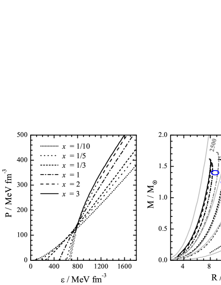
Figure 3: The SQM EOS and mass-radius relation of SSs with $x=1/10,1/5,1/3,1,2,3$. M(R) curves for lower boundaries defined in Fig. 1 with $x=1/5,1/3,1$ are also presented (grey lines in the right panel). Contours of the maximum rotation frequencies are given by the light grey curves (Gourgoulhon et al. 1999).

In addition, the surface electric field should be very strong near the bare quark surface of a strange star because of the mass difference of the strange quark and the up (or down) quark, which could play an important role in producing the thermal emission of bare strange stars by the Usov mechanism (Usov 1998; Usov 2001). Moreover, the strong electric field plays an essential role in forming a possible crust around a strange star, which has been investigated extensively by many authors (for a recent development, see Zdunik et al. 2001). Also it should be noted that this electric field has some important implications on pulsar radio emission mechanisms (Xu et al. 2001). Therefore it is very worthwhile to explore how the mass scaling influences the surface electric field of the stars, and possible related astronomical observations in turn may drop a hint on what the proper mass scaling would be. Adopting a simple Thomas-Fermi model, one gets the Poisson’s equation (Alcock et al. 1986):

$${d^{2}V\over dz^{2}}=\left\{\begin{array}[]{ll}{4\alpha\over 3\pi}(V^{3}-V_{\rm q}^{3})&z\leq 0,\\ {4\alpha\over 3\pi}V^{3}&z>0,\end{array}\right.$$ (12)

where $z$ is the height above the quark surface, $\alpha$ is the fine-structure constant, and $V_{\rm q}^{3}/(3\pi^{2}\hbar^{3}c^{3})$ is the quark charge density inside the quark surface. Together with the physical boundary conditions $\{z\rightarrow-\infty:V\rightarrow V_{\rm q},dV/dz\rightarrow 0;~{}~{}z\rightarrow+\infty:V\rightarrow 0,dV/dz\rightarrow 0\}$, and the continuity of $V$ at $z=0$ requires $V(z=0)=3V_{\rm q}/4$, the solution for $z>0$ finally leads to

$$V={3V_{\rm q}\over\sqrt{6\alpha\over\pi}V_{\rm q}z+4}~{}~{}({\rm for}~{}z>0).$$ (13)

The electron charge density can be calculated as $V^{3}/(3\pi^{2}\hbar^{3}c^{3})$, therefore the number density of the electrons is

$$n_{\rm e}={9V_{\rm q}^{3}\over\pi^{2}(\sqrt{6\alpha\over\pi}V_{\rm q}z+4)^{3}}$$ (14)

and the electric field above the quark surface is finally

$$E=\sqrt{2\alpha\over 3\pi}\cdot{9V_{\rm q}^{2}\over(\sqrt{6\alpha\over\pi}V_{\rm q}\cdot z+4)^{2}}$$ (15)

which is directed outward.

It is shown in Fig. 4 (take $x=1/3$ for example) that although the electric field near the surface is about $10^{18}$ V cm^-1, the outward electric field decreases very rapidly above the quark surface, and at $z\sim 10^{-8}$ cm, the field gets down to $\sim 5\times 10^{11}$ V cm^-1, which is of the order of the rotation-induced electric field for a typical Goldreich-Julian magnetosphere. To alter the mass scaling mainly has two effects: First, it affects a lot the surface electric field, and a small scaling parameter leads to an enhanced electric field. The change of electric field would be almost a order of magnitude large (from $10^{17}$ V cm^-1 to $10^{18}$ V cm^-1), which may have some effect on astronomical observations. Second, a larger scaling would slow the decrease of the electric field above the quark surface.

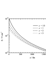
Figure 4: The electric field above the quark surface with $x=1/3,1,2,3$.

4 Conclusions

In this paper, we investigate the stability of SQM within a wide scaling range, i.e. from 0.1 to 3. We study also the properties of the SSs made of the matter. The calculation shows that the resulting maximum mass always lies between 1.5$M_{\odot}$ and 1.8$M_{\odot}$ for all the mass scalings chosen here. Strange star sequences with a linear scaling would support less gravitational mass, a change (increase or decrease) of the scaling parameter around the linear scaling would result in a higher maximum mass. Radii invariably decrease with the mass scaling; and then the larger the scaling, the faster the star rotates. In addition, the variation of the scaling may cause an order of magnitude change of the surface electric field, which may have some effect on astronomical observations.

References

- [1] Alcock, C., Farhi,E., & Olinto, A. 1986 Astrophys. J. 310, 261
- [2] Chakrabarty, S.; Raha, S., & Sinha, B. 1989 Phys. Lett. B, 229, 112
- [3] Chakrabarty, S. 1991, Phys. Rev. D, 43, 627
- [4] Chakrabarty, S. 1993, Phys. Rev. D, 48, 1409
- [5] Chakrabarty, S. 1996, Phys. Rev. D, 54, 1306
- [6] Dey, M., Bombaci, I., Dey, J., Ray, S., & Samanta, B. C. 1998, Phys. Lett. B, 438, 123; erratum 1999, Phys. Lett. B, 467, 303
- [7] Fowler, G. N., Raha, S. & Weiner, R. M. 1981, Z. Phys. C, 9, 271
- [8] Gourgoulhon, E., Haensel, P., Livine, R., Paluch, E., Bonazzola, S., and Marck, J.-A., 1999, A&A 349, 851
- [9] Lugones, G. & Horvath,J. E. 2003, Int. J. Mod. Phys. D, 12, 495
- [10] Peng, G. X., Chiang, H. Q., Zou, B. S., Ning, P. Z., & Luo, S. J. 1999, Phys. Rev. C, 62, 025801
- [11] Peng, G. X., Wen, X. J. & Chen, Y. D. 2006, Phys. Lett. B, 633, 313
- [12] Peng, G. X., Li, A., & Lombardo U. 2008, Phys. Rev. C, 77, 065807
- [13] Peng, G. X. 2009, private communication
- [14] Usov, V. V. 1998, Phys. Rev. Lett., 80, 230
- [15] Usov, V. V. 2001, ApJ, 550, L179
- [16] Wang, P. 2000, Phys. Rev. C, 62, 015204
- [17] Wen, X. J., Peng, G. X., & Chen, Y. D. 2007, J. Phys. G: Nucl. Part. Phys., 34, 1697
- [18] Xu, R. X., Zhang, B., & Qiao, G. J. 2001, Astroparticle Phys., 15, 101
- [19] Yao, W.-M. et al. 2006, J. Phys. G: Nucl. Part. Phys, 33, 1
- [20] Zdunik, J. L., Haensel, P., & Gourgoulhon, E. 2001, A&A, 372, 535
- [21] Zhang, Y., Su, R. K., Ying, S. Q. Ying., & Wang, P. 2001, Europhys. Lett, 56, 361
- [22] Zhang, Y., Su, R. K. 2002, Phys. Rev. C, 65, 035202
- [23] Zhang, Y., Su, R. K. 2003, Phys. Rev. C, 67, 015202
- [24] Zheng, X. P., Liu, X. W., Kang, M., & Yang,S. H. 2004, Phys. Rev. C, 70, 015803