Elicitation of Weibull priors

Summary

$-$ Based on expert opinions, informative prior elicitation for the common Weibull lifetime distribution usually presents some difficulties since it requires to elicit a two-dimensional joint prior. We consider here a reliability framework where the available expert information states directly in terms of prior predictive values (lifetimes) and not parameter values, which are less intuitive. The novelty of our procedure is to weigh the expert information by the size $m$ of a virtual sample yielding a similar information, the prior being seen as a reference posterior. Thus, the prior calibration by the Bayesian analyst, who has to moderate the subjective information with respect to the data information, is made simple. A main result is the full tractability of the prior under mild conditions, despite the conjugation issues encountered with the Weibull distribution. Besides, $m$ is a practical focus point for discussion between analysts and experts, and a helpful parameter for leading sensitivity studies and reducing the potential imbalance in posterior selection between Bayesian Weibull models, which can be due to favoring arbitrarily a prior. The calibration of $m$ is discussed and a real example is treated along the paper.

Key Words

$-$ subjective prior elicitation, Weibull distribution, expert opinion, virtual data, posterior prior.

1 Introduction

The versatile Weibull $\cal W(\eta,\beta)$ distribution, with density function

$$f_{W}(t|\eta,\beta) = \frac{\beta}{\eta}\left(\frac{t}{\eta}\right)^{\beta-1}\exp\left\{-\left(\frac{t}{\eta}\right)^{\beta}\right\}\ \mathds{1}_{\{t\geq 0\}}$$

$(\eta,\beta)\in(0,\infty)^{2}$, is one of the most popular distributions in reliability and risk assessment (RRA) and many other fields, mainly chosen for modelling the lifetime $T$ of an industrial system or component $\Sigma$ Tsionas, (2000). In real-life studies, a Bayesian framework has often been highlighted when expert knowledge is available on $\Sigma$ and observed lifetime data ${\bf t_{n}}=t_{1},\ldots,t_{n}$ are small-sized and possibly contain missing or censored values Bacha et al., (1998). Such contexts are usually encountered in industrial studies, especially when economical opportunities imply replacing a range of components at the same time, although they could have carried on running, and lead to “polluted” (e.g., censored) lifetime data. In those cases, all relevant sources of knowledge as expert opinion must be taken into account.

Therefore, numerous authors Singpurwalla, N.D. and Song, M.S. (1986); Singpurwalla, N.D. (1988); Berger, J.O. and Sun, D. (1993) have focused their work on the elicitation of a joint prior measure $\pi(\eta,\beta)$ that formalizes the expert knowledge, in order to integrate some decision-making function over the joint posterior distribution of these parameters, with density

$$\pi(\eta,\beta|{\bf t_{n}}) = \frac{{\cal{L}}({\bf t_{n}};\eta,\beta)\ \pi(\eta,\beta)}{\displaystyle\iint_{I\!\!R^{2}_{+}}{\cal{L}}({\bf t_{n}};\eta,\beta)\ \pi(\eta,\beta)\ d\eta d\beta},$$

where ${\cal{L}}({\bf t_{n}};\eta,\beta)$ denotes the data likelihood. There are two main difficulties using the Weibull distribution. First, its only conjugate prior distribution is continuous-discrete Soland, R. (1969) and remains difficult to justify in real problems Kaminskiy, M.P., and Krivtsov, V.V. (2005). Second, the meanings of scale parameter $\eta$ and shape parameter $\beta$ greatly differ. Their values and correlation remain hard to assess by non-statistician experts, even though historical results Lannoy, A. and Procaccia, H. (2001) can be used to provide preferential values as a function of the behavior of the studied system. The methods proposed by the previous authors can suffer from this second defect and be applicable with difficulty. Therefore Kaminskiy & Krivtsov Kaminskiy, M.P., and Krivtsov, V.V. (2005) recently provided a simple procedure to elicit a prior $\pi(\eta,\beta)$ using expert knowledge about the mean and standard deviation of the cumulative distribution function (cdf) $F_{W}$. They insisted on the fact that these values are easier to assess than parameter values.

However, especially in sensitive areas like nuclear safety UNW89 , resorting to a Bayesian framework for reliability-based decision-helping implies defending the metholodology of prior elicitation in front of control authorities, the traditional difficulty being the treatment of its subjective aspects EFR86 . According to most wishes expressed by decisionners in our practice, the elicitation of a “defendable” prior $\pi(\theta)$ (of any model parametrized by $\theta$ and not only Weibull) should respect the following items: (a) the quantity of subjective information can be directly compared, in terms of percentage, to the quantity of objective (data) information; and (b) the elicited prior must be unique.

One could add to this list other wishes as the practical handling of the prior (explicit features and easy sampling), which is of importance for sensitivity studies. Note that the first item requires to give a clear sense to the words “quantity of information”. Statistical definitions like inverse Fisher matrices or Shannon entropies are often too technical to be directly accessible to decisionners.

This article addresses those concerns. In the sequel, we consider an alternative elicitation of $\pi(\eta,\beta)$ defined as the reference posterior of virtual data of size $m$ but calibrated from lifetime magnitudes directly given by experts, pursuing the worry of realism expressed by Kaminskiy & Krivtsov Kaminskiy, M.P., and Krivtsov, V.V. (2005). Since the virtual size corresponds to an intuitive measure of prior uncertainty, ratios of virtual and observed data sizes bring an understandable sense to the notion of “relative quantity of information”. It can appear simpler than standard deviations (or other typical statistical uncertainty measures) to discuss with non-statistician experts and, especially, lead to more transparent choices to decisionners.

The structure of the paper is as follows. The full prior elicitation is detailed in (the largest) Section 2. This methodological section focuses on the calibration of hyperparameters, the aggregation of independent expert opinions and the equitability issues between Bayesian Weibull models. Posterior computation is considered in Section 3. A numerical application on a real case-study is treated along the paper to illustrate the methodology. A Discussion section ends the paper, presenting alternative results and some avenues for future research.

2 Prior elicitation

2.1 Principle

The central idea of prior elicitation comes from a simple vision of informative expert opinion already suggested by Lindley Lindley (1983). We suggest to consider that a perfect expert opinion should be, roughly speaking, similar to a real data survey, and provide an independent and identically distributed (i.i.d.) sample ${\bf\tilde{t}_{m}}=(\tilde{t}_{1},\ldots,\tilde{t}_{m})$ of lifetime data. Now, let $\pi^{J}$ be a well-recognized formal representation of ignorance (namely, a noninformative prior), perceived as a reference benchmark measure on the parameter space. Assuming ${\bf\tilde{t}_{m}}$ is known, the corresponding prior $\pi$ should be the posterior distribution with density $\pi^{J}(\eta,\beta|{\bf\tilde{t}_{m}})$.

Posterior priors.

Priors built as virtual posteriors present some advantages in subjective Bayesian analysis. First, they are unique since only defined by $\pi^{J}$ and the likelihood (often historically chosen in experiments). Second, the correlation between parameters is automatically assessed through the Bayes rule. Third, as said before, the ratio between the numbers of virtual and real data helps to yield an understandable answer to the (often unclear) question “what is the ratio between subjective and objective information” asked by cautious decision-makers. Finally, the aggregation of independent expert opinions is simply carried out through successive Bayes rules, the consensus virtual sample being an aggregation of all virtual data. This avoids choosing opinion pooling rules which can suffer from paradoxes oha06b .

Maybe the most famous of such elicited priors is Zellner’s $g-$prior Zellner, A. (1986). Among others, Clarke CLA96 , Neal Neal (2001), Kárny et al. Kárny et al. (2003), Lin et al. Lin, X., Pittman, J. and Clarke, B. (2007) and Morita et al. Morita et al. (2007) examined various quantification of priors using virtual data. Kontkanen et al. Kontkanen et al. (1998) considered virtual data as practical tools for eliciting priors for Bayesian networks which may require automation in the treatment of their parameters.

However, because of various factors, especially subjective ones, the sample ${\bf\tilde{t}_{m}}$ is not directly elicitable from an expert, and his or her information on lifetime $T$ must be summarized through questioning processes oha06b . This type of elicitation remains simple for distributions belonging to the natural exponential family, for which the resulting posterior priors are conjugate (cf. PRE03 , $\S$ 5.3.3), because the virtual sample can be replaced by exhaustive statistics. In the continuous Weibull case, unfortunately, the only exhaustive statistic is the full virtual likelihood. Therefore the questioning must be oriented such that it allows the calibration of nonexhaustive virtual statistics.

Expert questioning.

In a concern of realism, following the ideas promoted by Kadane & Wolfson kad98 and especially Percy PER02 in the field of RRA, we consider that an expert is mainly capable of providing observable information on $T$, unconditionally to $(\eta,\beta)$. Indeed, the experts are usually not statisticians and should yield information independently from any parametrization choice (and even from any sampling model choice) made by a Bayesian analyst Kárny et al. (2003). In other terms we assume that any realistic statistical summary of an expert opinion should be defined with respect to its associated prior predictive density, namely the prior density of plausible lifetime values

$$f_{\pi}(t) = \iint_{I\!\!R^{2}_{+}}f_{W}(t|\eta,\beta)\pi(\eta,\beta)\ d\eta d\beta.$$ (1)

The density form of de Finetti’s representation theorem def74 is then invoked to ensure the unicity of priors elicited in this way, under mild conditions of exchangeability for sequences of values $t_{1},\ldots,t_{n},\ldots$ See Press PRE03 , $\S$ 10.5, for more precisions. Linking typical magnitudes of the observable variable $T$ with statistical specifications can be made through decision-theoretical arguments. In the following, we consider experts who can answer to a question similar to the following one:

Can you give estimates of relative costs $(c_{1},c_{2})$ linked to two reliability-based decisions induced by the two mutually exclusive events $T\leq t_{\alpha}$ and $T>t_{\alpha}$?

provided $t_{\alpha}$ is given by the analyst (to improve the phenomenon anchoring of the expert and diminish subjective bias, cf. TVE74 ) and denoting $\alpha=c_{1}/(c_{1}+c_{2})\in[0,1]$. Doing so, following the standard criterion of decision theory, namely the expected utility Robert, C.P. (2001), the analyst interprets $t_{\alpha}$ as the minimizer of the predictive Bayes risk

$${t}_{\alpha} = \arg\min\limits_{t_{0}>0}\int_{0}^{\infty}\Lambda(t_{0},t|c_{1},c_{2})f_{\pi}(t)\ dt.$$

defined by some loss function $\Lambda(t_{0},t|c_{1},c_{2})$ between the choice $T=t_{0}$ and the unknown truth $T=t$, inflicting $c_{1}$ to the event $t\leq t_{0}$ (underestimation) and $c_{2}$ to the contrary event $t>t_{0}$ (overestimation). The common choice

$$\Lambda(t_{0},t|c_{1},c_{2}) = |t-t_{0}|\left(c_{1}\cdot 1_{\{t\leq t_{0}\}}+c_{2}\cdot 1_{\{t>t_{0}\}}\right),$$

which underlies the analyst wants to penalize similarly small and large misestimations Robert, C.P. (2001), leads to $t_{\alpha}$ taking the sense of the $\alpha-$order prior predictive percentile

$$P_{\pi}(T<{t}_{\alpha}) = \int_{0}^{{t}_{\alpha}}f_{\pi}(t)\ dt\ =\ \alpha.$$ (2)

Therefore an alternative equivalent query is, perhaps simpler, what is the risk $\alpha$ for $\Sigma$ to break down before $t_{\alpha}$?

In the following, we assume finally that for each available expert, a unique specified couple $(t_{\alpha},\alpha)$ among all elicitable can be considered as his or her most trustworthy specification (MTS) and must be exactly respected in the effective predictive prior modelling. Various reasons can be invoked for this. First, one cannot hope to elicit a prior $\pi(\eta,\beta)$ such that an arbitrary large number of specified couples $(t_{\alpha},\alpha)$ be exactly respected together, because of the limited flexibility of parametric distributions (Berger 1985 Berger, J.O. , chap. 3). Second, a MTS often appears as a reality since experts have usually more difficulty to speak in terms of extreme values rather than values close to the median behavior oha06b . Typically, they can share a similar MTS while their extremes can differ (see Example 2.1). Other arguments can be related to decision-making: a cautious, conservative couple $(t_{\alpha},\alpha)$ can be favored by the analyst since the posterior analysis is focused on percentiles of higher, more critical orders.

Example 1. Table 1, already used in Bousquet, N. (2006), summarizes two prior opinions about the lifetime $T$ (in months) of a device belonging to the secondary water circuit of French nuclear plants. According to a large consensus in the RRA field, $T$ is assumed to be well described by a Weibull distribution. Giving a normative sense to extreme events ($90\%$ credibility), these experts were not questionned at the same level of precision. ${\cal{E}}_{1}$ is a nuclear operator and spoke about a particular component, in terms of replacement costs. Conversely, ${\cal{E}}_{2}$ is a component vendor whose opinion took into account a variety of operating conditions. Costs invoked here were mainly related to mass production. Therefore the two experts can be considered independent. Hence the common median appears as a robust specification and is chosen as the MTS for both.

	Credibility intervals (5%,95%)	Median value
expert ${\cal{E}}_{1}$	[200,300]	250
expert ${\cal{E}}_{2}$	[100,500]	250

Table 1: Expert opinions about the lifetime $T$ of a nuclear device (in months).

2.2 A comfortable prior form

Let us choose $\pi^{J}$ as the Jeffreys prior for Weibull. In more general Bayesian settings, Sun Sun (1997) proposed to favor the Berger-Bernardo reference prior Berger, J.O and Bernardo, J.M. (1992) since it has slightly better properties of frequentist posterior coverage. But this prior requires at least $m\geq 2$ to get proper posteriors. This would be limiting in practice, when $m$ is chosen small as it could be expected in cautious subjective assessments. Moreover, expert knowledge exerts here itself on $T$ and not on any Weibull parametrization, therefore it seems relevant that a benchmark $\pi^{J}$ be parametrization-invariant. See CLA96 for a straightforward defence of Jeffreys’ prior in related problems, where a subjective posterior has to be compared in information-theoretic terms to an objective posterior. Thus we consider

$$\pi^{J}(\eta,\beta) \propto \eta^{-1}\mathbbm{1}_{\{\eta\geq 0\}}\mathbbm{1}_{\{\beta\geq\beta_{0}\}}$$

where $\beta_{0}\geq 0$ is assumed to be fixed by objective reasons, like physical constraints. For instance, a reliability study focusing on industrial components submitted to aging leads to choose $\beta_{0}=1$ as explained in Bacha (1998) Bacha et al., (1998), since involving a time-increasing failure rate. Without particular constraint, $\beta_{0}=0$. Scale invariance imposes no other lower bound than 0 for $\eta$.

Denote ${\cal{GIG}}(a,b,\gamma)$ the generalized inverse gamma distribution with density

$$f(x) = \frac{b^{a}\gamma}{\Gamma(a)}\frac{1}{x^{a\gamma+1}}\exp\left(-\frac{b}{x^{\gamma}}\right)\mathbbm{1}_{\{x\geq 0\}}.$$

Reparametrizing $x$ in $\mu=x^{-\gamma}$, $\mu\sim{\cal{G}}(a,b)$. Then our ideal prior is $\pi(\eta,\beta)=\pi(\eta|\beta)\pi(\beta)$, such that

$$\eta|\beta \sim {\cal{GIG}}\left(m,b({\bf\tilde{t}_{m}},\beta),\beta\right),$$ (3)

$$\pi(\beta) \propto \frac{\beta^{m-1}\ }{{b^{m}({\bf\tilde{t}_{m}},\beta)}}\ \exp\left(m\frac{\beta}{\beta({\bf\tilde{t}_{m}})}\right)\mathbbm{1}_{\{\beta\geq\beta_{0}\}}$$ (4)

with ${b({\bf\tilde{t}_{m}},\beta)=\sum_{i=1}^{m}\tilde{t}^{\beta}_{i}}$, and $\beta({\bf\tilde{t}_{m}})=m(\sum_{i=1}^{m}\log\tilde{t}_{i})^{-1}$. Both distributions are proper for all $m>0$. The unknown virtual unsufficient statistics $b({\bf\tilde{t}_{m}},\beta)$ and $\beta({\bf\tilde{t}_{m}})$ must be replaced in function of available expert information. The linkage between the prior form promoted in (3-4) and a MTS $(t_{\alpha},\alpha)$ elicitable for a given expert can be done as explained in the next proposition (proved in Appendix) and its corollary.

Proposition 1. For $\alpha\in]0,1[$ and ${t}_{\alpha}>0$, define the function $b_{\alpha}:\ I\!\!N^{*}\times I\!\!R^{*}_{+}$ by

$$b_{\alpha}(m,\beta) = \left({(1-\alpha)^{-1/m}-1}\right)^{-1}{t_{\alpha}}^{\beta}.$$ (5)

Then $b_{\alpha}(m,\beta)$ is the only $\beta-$continuous function such that, being substituted to $b({\bf\tilde{t}_{m}},\beta)$ in (3), Equation (2) is verified almost surely.

An immediate and pleasant consequence of replacing deterministic expression $b({\bf\tilde{t}_{m}},\beta)$ by $b_{\alpha}(m,\beta)$ is that $\pi(\beta)\propto\beta^{m-1}\exp\left(-m\beta\log t_{\alpha}+m{\beta}/{\beta({\bf\tilde{t}_{m}})}\right)\mathbbm{1}_{\{\eta\geq 0\}}$. We recognize here the general term of a gamma distribution truncated in $\beta_{0}$. Finally the resulting prior is

$$\eta|\beta \sim {\cal{GIG}}\left(m,b_{\alpha}(m,\beta),\beta\right),$$ (6)

$$\beta \sim {\cal{G}}\left(m,\frac{m}{\widetilde{\beta}(m)}\right)\mathds{1}_{\{\beta\geq\beta_{0}\}}$$ (7)

where $\widetilde{\beta}(m)=\left(\log t_{\alpha}-\beta^{-1}({\bf\tilde{t}_{m}})\right)^{-1}$. This result deserves some technical remarks.

(i)

The joint prior propriety imposes $\beta^{-1}({\bf\tilde{t}_{m}})<\log t_{\alpha}$, namely $\prod_{i=1}^{m}\tilde{t}_{i}<t^{m}_{\alpha}$.

(ii)

The joint prior (6-7) can remain proper for all $m$ extended on the half-line $I\!\!R^{*}_{+}$. Thus fuzzy or doubtful experts can be graded using $m\leq 1$. This might be valuable if a group of $P$ experts is considered as yielding less information than $P$ i.i.d. data, for instance because they are suspected of mutual influence.

(iii)

The ${\cal{GIG}}(a,b,\gamma)$ distribution was firstly used by Berger & Sun Berger, J.O. and Sun, D. (1993), $b$ being assessed independently of $\beta$. However, this choice was made only because of the posterior conjugate properties conditionally to $\beta$ (see $\S$ 3), and no meaning was given to the hyperparameters. Authors like Tsionas Tsionas, (2000) adopted similar approaches.

2.3 Prior calibration

In addition to the MTS needed to define the prior form (6-7), supplementary prior information must be available for the calibration of $(m,\widetilde{\beta}(m))$. In the two following paragraphs we consider some cases commonly encountered in RRA.

2.3.1 Calibrating $\widetilde{\beta}(m)$

In RRA, it can occur that the analyst benefits from qualitative information on the nature of aging of $\Sigma$. For instance, assuming $\beta_{0}=0$, if the expert can answer the question what is the probability $0<\alpha_{\beta_{e}}<1$ that $\Sigma$ is submitted to aging?, one would have a priori $P(\beta<\beta_{e})=1-\alpha_{\beta_{e}}$ with $\beta_{e}=1$ and consequently

$$\widetilde{\beta}(m) = 2m\beta_{e}/\chi^{2}_{2m}(1-\alpha_{\beta_{e}})$$ (8)

where $\chi^{2}_{m}(q)$ is the $q-$order percentile of the $\chi^{2}_{m}$ distribution. Other similar questions can be asked over accelerated aging (${\beta_{e}}=2$) and extreme cases (${\beta_{e}}=5$) reflecting inconceivable kinetics of aging in industrial applications Bacha et al., (1998); Lannoy, A. and Procaccia, H. (2001). Otherwise, databases of typical $\beta$ values (e.g., http://www.barringer1.com/wdbase.htm) can be used to quantify some alternative features of the gamma prior.

However, most frequently (as in Example 2.1), other quantitative information is available under the form of a single or several credibility intervals, one of whose bounds is the previously chosen MTS. We consider $p\geq 1$ supplementary (non-independent) specifications $\Omega_{p}=\{t_{\alpha_{i}},\alpha_{i}\}_{i\in\{1,\ldots,p\}}$, sorted by increasing order ($\alpha_{i}<\alpha_{i+1}$ and $t_{\alpha_{i}}<t_{\alpha_{i+1}}$). Given $m$, calibrating $\widetilde{\beta}(m)$ under those predictive constraints can be done by minimizing a distance ${\cal{D}}_{m}(f^{*},f_{\pi})$ where $f^{*}$ is a pdf of $T$ respecting exactly the MTS and the specifications listed in $\Omega_{p}$. To avoid dealing with the infinite number of possible $f^{*}$, we adopt the approach proposed by Cooke Cooke (1991): ${\cal{D}}$ is chosen as the discrete Kullback-Leibler loss function between required and elicited marginal features

$${\cal{D}}_{m}(f^{*},f_{\pi}) = \sum\limits_{i=0}^{p}P_{f^{*}}\left(T\in[t_{\alpha_{i}},t_{\alpha_{i+1}}]\right)\log\frac{P_{f^{*}}\left(T\in[t_{\alpha_{i}},t_{\alpha_{i+1}}]\right)}{P_{f_{\pi}}\left(T\in[t_{\alpha_{i}},t_{\alpha_{i+1}}]\right)}$$ (9)

$$= \sum\limits_{i=0}^{p}(\alpha_{i+1}-\alpha_{i})\log\frac{(\alpha_{i+1}-\alpha_{i})}{\left(\alpha^{(e)}_{i+1}-\alpha^{(e)}_{i}\right)}$$

where $t_{\alpha_{0}}=0$, $t_{\alpha_{p+1}}=\infty$, $\alpha_{0}=\alpha^{(e)}_{0}=0$, $\alpha_{p+1}=\alpha^{(e)}_{p+1}=1$, and for $i\in\{1,\ldots,p\}$

$$\alpha^{(e)}_{i} = {\displaystyle\iint F_{W}\left(t_{\alpha_{i}}|\eta,\beta\right)\pi(\eta,\beta)\ d\eta d\beta}.$$

The convexity of this loss function in its argument $\pi$ and, given $m$ and $\beta$, the one-to-one continuous correspondence between $\pi(\beta|\widetilde{\beta}(m))$ and $\widetilde{\beta}(m)$ allows for a unique solution of the calibration problem

$$\widetilde{\beta}^{*}(m) = \arg\min\limits_{\pi(.|\widetilde{\beta}(m))}{\cal{D}}_{m}(f^{*},f_{\pi}).$$

From (8), estimating $\widetilde{\beta}^{*}(m)$ is similar to select $\alpha_{\beta_{e}}=0.5$ and minimizing (9) in the prior median $\beta^{*}_{e}$. This provides a direct view of the underlying aging and numerical estimations were found slightly more robust than those of the prior mean, or those of the best order $\alpha^{*}_{\beta_{e}}$ if, conversely, $\beta_{e}$ is fixed. Therefore we temporarily note $\widetilde{\beta}(m)=\widetilde{\beta}_{m}(\beta_{e})$. For a given $m$, a combination of golden section search and successive parabolic interpolation BRE73 can achieve a robust optimization of $\beta_{e}$, provided the $\alpha^{(e)}_{i}$ are smoothly computed at each step of the algorithm. A smooth Monte Carlo estimation can be obtained using a unique importance sampling run $\beta_{1},\ldots,\beta_{M}\sim{\cal{G}}(m,m/\beta_{e,0})$, with large $M$, where $\beta_{e,0}$ is a chosen starting point:

$$\alpha^{(e)}_{i}\left(m,\beta_{e}\right) \simeq {\displaystyle 1-\left(\frac{\beta_{e,0}}{\widetilde{\beta}_{m}(\beta_{e})}\right)^{m}\frac{1}{M}\sum\limits_{j=1}^{M}\left[{\left(1+\frac{t^{\beta_{j}}_{\alpha_{i}}}{b_{\alpha}(m,\beta_{j})}\right)}{\exp\left(\beta_{j}\left[\frac{1}{\widetilde{\beta}_{m}(\beta_{e})}-\frac{1}{\beta_{e,0}}\right]\right)}\right]^{-m}}.$$

Note that

$$\mbox{Err}(m)={\cal{D}}_{m}\left(f^{*},f_{\pi\left(.|\widetilde{\beta}^{*}(m)\right)}\right)$$

measures the expert incoherency with respect to the predictive Weibull distribution, given a virtual sample of size $m$ in agreement with the expert opinion. If $\mbox{Err}(m)$ remains large for many $m$, the Weibull choice for the virtual data (and therefore for any real dataset, provided the expert is relevant for the problem) is at least debatable, not to say probably inappropriate.

2.3.2 Calibrating $m$

The calibration of $m$ must be adapted to the experimental context. A decisionner can impose a given virtual size to improve the clarity of the posterior result. For instance, Marin and Robert MAR10 proposed to give to the virtual size parameter of Zellner’s $g-$prior (on regressors of a gaussian linear regression problem) the value $m=1$ by default. In a similar context, another possibility, proposed by Celeux et al. CEL06 and Liang et al. LIA08 among others, is to establish an upper hierarchical level in the Bayesian model by considering $m$ as a random variable for which a weakly informative prior must be elicited. A last possibility is to use $m$ as a discussion tool between the analyst and the expert, since the meaning of $m$ is understandable outside the statistical field. Some heuristic methods in this sense are discussed in Bousquet, N. (2006).

However our aim as a Bayesian analyst is mainly to measure the strenght of the expert opinion (assumed being correctly reflected through the prior modelling) through $m$. Besides, when the experts are no longer questionable and only a summary of their past opinions remains available, it seems somewhat difficult to elicit a hyperprior on this parameter. Then we suggest that $m$ should be integrated as the minimizer of the expert incoherency risk, namely

$$m^{*} = \arg\min_{m\geq 0}\mbox{Err}(m).$$

It is the analyst’s decision to minimize this risk on $I\!\!N^{*}$ (not to loose the virtual size meaning) or $I\!\!R^{*}_{+}$. In our experiments we chose $I\!\!R^{*}_{+}$ to get the closest prior to the expert opinion. Obviously, one can avoid eliciting a too informative prior by limiting the minimization domain to $(0,n]$.

Example 2.(pursuing Example 2.1). For a continuum of values of $m$, we display on Figures 4 and 4 the optimized $\tilde{\beta}^{*}(m)$ and the corresponding risk $\mbox{Err}(m)$, respectively, for both experts. In both cases, the shape of $m\mapsto\mbox{Err}(m)$ allows for a unique solution $m^{*}$. We find $m^{*}=3.36$ for expert ${\cal{E}}_{1}$ and $m^{*}=2.50$ for expert ${\cal{E}}_{2}$. This is logical since ${\cal{E}}_{1}$ is more informative than ${\cal{E}}_{2}$. However, all values $\tilde{\beta}^{*}(m)$ for expert ${\cal{E}}_{1}$ appear unrealistic in an industrial physical context, testifying from exponential uncontrolled aging, assuming the Weibull model is correct. Especially, the calibrated $\tilde{\beta}^{*}(m^{*})=16.5$, which induces a peaked normal behavior of the prior predictive distribution (cf. DOD06 ). On the contrary, the opinion of expert ${\cal{E}}_{2}$ remains physically plausible ($\tilde{\beta}^{*}(m^{*})=4.9$) although the underlying aging is still strong. The corresponding coverage matching error $|1-({\alpha^{(e)}_{t_{1}}-\alpha^{(e)}_{t_{2}}})/{90\%}|$, where $\alpha^{(e)}_{t_{i}}$ is the effective percentile order for $t_{i}\in\{100,200\}$ or $t_{i}\in\{300,500\}$, is plotted in Figure 4 and shows a good adequacy between the wanted and effective credible domains: less than 5% error in all cases, and less than 0.2% and 0.004% when choosing the calibrated $m^{*}$, for experts ${\cal{E}}_{1}$ and ${\cal{E}}_{2}$ respectively.

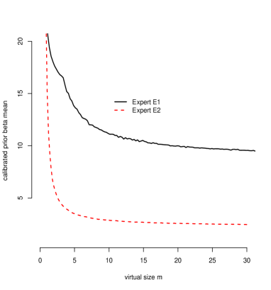
Figure 1: Calibrated prior mean $\tilde{\beta}^{*}(m)$ in function of $m$, for each expert opinion summarized in Table 1.

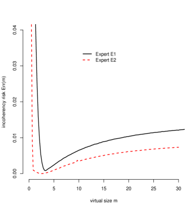
Figure 2: Expert incoherency risk $\mbox{Err}(m)$ in function of $m$, for each expert opinion summarized in Table 1. Minima of plots indicate calibrated values $m^{*}$.

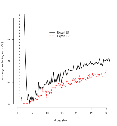
Figure 3: Prior predictive coverage matching error in percentage.

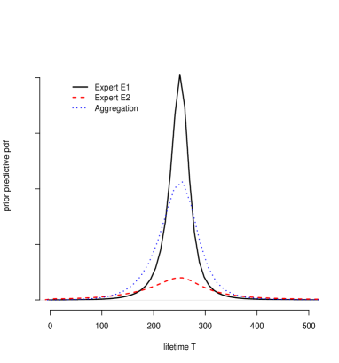
Figure 4: Prior predictive densities for both expert opinions and the aggregation of opinions.

2.4 Aggregation of independent expert opinions

In cases when the aggregation of $i=1,\ldots,p$ priors is chosen as a way to avoid interacting biases in a group of experts, it yields a similar information to that carried by a global virtual sample, which is the union of all experts’ samples $\bf\tilde{t}_{m_{i}}$. Because they are not explicitly known, one may use a concatenation of known samples ${\bf\tilde{s}_{{m_{1}}}},\ldots,{\bf\tilde{s}_{{m_{p}}}}$ from another model ${\cal{M}}(\eta,\beta)$ such that their parametric likelihood $(\eta,\beta)\mapsto\ell({\bf\tilde{s}_{m_{1}}},\ldots|\eta,\beta)$ leads to the same inference as the whole virtual sample. Indeed, we can show easily (cf. Lemma Proof of Proposition 2.2. in Appendix) that

$$\pi^{J}\left(\eta,\beta|{\bf\tilde{t}_{m_{1}}},\ldots,{\bf\tilde{t}_{m_{p}}}\right) = \pi^{J}_{{\cal{M}}}\left(\eta,\beta|{\bf\tilde{s}_{m_{1}}},\ldots,{\bf\tilde{s}_{m_{p}}}\right)\ \propto\ \pi^{J}(\eta,\beta)\prod\limits_{i=1}^{p}\ell({\bf\tilde{s}_{m_{i}}}|\eta,\beta).$$

Next proposition, proved in Appendix, gives an example of such a likelihood (said virtual likelihood) for a single expert opinion.

Proposition 2. Consider ${\bf\tilde{s}_{m}}=(k_{\alpha,m},\beta_{t_{\alpha},m})$, where $k_{\alpha,m}=({(1-\alpha)^{-1/m}-1})^{-1}$ and $\beta_{t_{\alpha},m}={\widetilde{\beta}(m)}/{(1+\widetilde{\beta}(m)\log t_{\alpha})}$, as a sample whose components follow independently the ${\cal{G}}(m,m(t_{\alpha}/\eta)^{\beta})$ and ${\cal{IG}}(m,m\beta)$ distributions, respectively. Then it defines a virtual likelihood for an expert opinion summarized by $(t_{\alpha},\alpha,\widetilde{\beta}(m))$.

After simple algebra, the resulting prior for all expert opinions is of the same form (6-7), for which (respecting intuition) $m=\sum_{i=1}^{p}m_{i}$, $b_{\alpha}(m,\beta)=\sum_{i=1}^{p}b_{\alpha_{i}}(m_{i},\beta)$ and

$$\widetilde{\beta}(m) = m\left(\sum\limits_{i=1}^{p}\frac{m_{i}}{\widetilde{\beta}_{i}(m_{i})}\right)^{-1}.$$

Example 3.(pursuing Example 2.3.2). Denote $(\pi_{1},\pi_{2})$ the priors calibrated in Example 2.3.2 for each expert. Denote $\pi_{3}$ the aggregating prior. Although $\pi_{3}$ appears less relevant than $\pi_{2}$ with respect to a Weibull model in a RRA context, we have no supplementary information to weight the strenght of its corresponding virtual sample in $\pi_{3}$. Then, by defect, $\pi_{3}$ is defined by

$$m = 5.86,\ \ \ \ \ b_{\alpha}(\beta)\ =\ 7.33\cdot(250)^{\beta},\ \ \ \ \ \widetilde{\beta}\ =\ 8.30.$$

Corresponding prior predictive densities are plotted on Figure 4. As it could be expected, the aggregation prior realizes a trade-off between the two priors in the sense it favors the common median according to an intermediate peak, due to the addition of spread virtual data (expert ${\cal{E}}_{2}$) to concentrated virtual data (expert ${\cal{E}}_{1}$).

2.5 Prior equitability among Weibull models

Weibull models are often used as bricks for more general reliability models, like competing risk models BER06 or mixtures Tsionas (2002). Especially, a usual challenge in RRA to choose between exponential and Weibull models. Since the exponential is nested into the Weibull model ($\beta=1$), a simple likelihood ratio test can be carried out in the frequentist framework. A Bayes factor is also easy to compute in our framework. Logically, both models share the same prior elicitation method, with the same MTS.

Then denote $(m_{E},m_{W})$ the two corresponding virtual sizes, $(\pi_{E},\pi_{W})$ the associated priors, and assume the more complex prior $\pi_{W}$ has been calibrated. How should $m_{E}$ be calibrated such that none of the prior Bayesian models is arbitrarily favored in absence of real data? The problem of defining such a prior equitability to reduce bias in posterior selection has been considered by many authors (see CEL06 for a review), who proposed several rules. Celeux et al. (2006) CEL06 gave decisive arguments to calibrate $\pi_{E}$ such that it minimizes the Kullback-Leibler divergence between predictive distributions

$$m^{*}_{E} = \arg\limits_{m_{E}}\min\mbox{KL}\left(f_{\pi_{W}},f_{\pi_{E}}(.|m_{E})\right)$$

where, after simple algebra,

$$f_{\pi_{E}}(t|m_{E}) = m_{E}\frac{b_{\alpha}^{m_{E}}(m_{E},1)}{(b_{\alpha}(m_{E},1)+t)^{m_{E}+1}}.$$

A unique Monte Carlo sampling of $f_{\pi_{W}}$ can be used to get a smooth description of the KL divergence and its derivative in $m$, so that a coupled Newton-Raphson method can provide a good estimate of $m^{*}_{E}$. This strategy can be carried out on more complex Weibull models, sorting them through their decreasing order of degree of freedom. If all authors have emphasized the difficulty of this task when nested models are nonconjugate with multidimensional parameters, our framework leads to a rather simple optimization.

Example 4.(pursuing Example 2.4). For various values of $m_{E}$, the KL divergence is plotted for expert ${\cal{E}}_{2}$ on Figure 6. The KL convexity allows for a unique solution $m^{*}_{E}=6.70$. When modifying $m_{W}$, the correspondence between $m_{W}$ and $m^{*}_{E}$ is plotted in Figure 6. A similar calculus for expert ${\cal{E}}_{1}$ leads to a very high value of $m^{*}_{E}$ (upper than 200), because any exponential predictive distribution cannot approximate well a peaked normal distribution. An exponential assumption thus appears deeply irrelevant for this expert opinion.

It could have been expected that $m^{*}_{E}\leq m_{W}$ since the more complex Weibull model should need more data that the exponential one to describe the same prior information. However, the model simplification reduces the global uncertainty in the effective prior predictive distribution. This has a direct impact on the virtual size $m_{E}$ which varies inversely to uncertainty measures.

Figure 5: KL distance between prior predictive Weibull and exponential distributions dedicated to expert ${\cal{E}}_{2}$’s opinion, in function of the exponential virtual size $m_{E}$. The minimum is reached in $m^{*}_{E}$.

Figure 6: Correspondence between Weibull and exponential virtual sizes $(m_{W},m^{*}_{E})$ for the expert ${\cal{E}}_{2}$’s opinion.

3 Posterior inference

Thanks to the considerable development of numerical sampling methods, posterior computation is no longer burdensome in two-dimensional cases. Nonetheless, the conditional conjugation prior properties simplify the work of the Bayesian analyst. To be general in the RRA area and in relation with Example 3, we assume that observed data ${\bf t_{n}}=(t_{1},\ldots,t_{n})$ contain $r$ i.i.d uncensored data $t^{(u)}_{1},\ldots,t^{(u)}_{r}$ and $n-r$ right-censored data. Denote $\delta_{\bf t_{n}}(\beta)=\sum_{i=1}^{n}t^{\beta}_{i}$ and $\beta_{\bf t_{n}}=r/\sum_{j=1}^{r}\log t^{(u)}_{i}$. Then the joint posterior distribution has density $\pi(\eta|\beta,{\bf t_{n}})\pi(\beta|{\bf t_{n}})$, such that

$$\eta|\beta,{\bf t_{n}} \sim {\cal{GIG}}\left(m+r,b(m,\beta)+\delta_{\bf t_{n}}(\beta),\beta\right),$$

$$\pi(\beta|{\bf t_{n}}) \propto \frac{b^{m}_{\alpha}(m,\beta)\beta^{m+r-1}}{\left(b_{\alpha}(m,\beta)+\delta_{\bf t_{n}}(\beta)\right)^{m+r}}\ \exp\left\{-\beta\left(\frac{m}{\tilde{\beta}(m)}-\frac{r}{\beta_{\bf t_{n}}}\right)\right\}\ \mathbbm{1}_{\{\beta\geq\beta_{0}\}}.$$

It is enough to obtain approximate posterior sampling of $\beta$ to get a complete joint sampling (using Gibbs sampling for $\eta$ conditional to $\beta$). This can be made efficiently via the adaptive rejection sampling algorithm from Gilks and Wild GIL92 . In a noninformative context (i.e., when $m\xrightarrow[]{m>0}0^{+}$) which can be easily adapted to a more general setting, Tsionas Tsionas, (2000) proposed a gamma instrumental distribution $\rho(\beta)$ whose mean is calculated to optimize the acceptance rate.

A particular attention must be paid to the existence of posterior moments, especially the first one which defines the Mean Time To Failure (MTTF) in a RRA context. The conditional posterior mean of $\eta$ is

$$\mbox{E}[\eta|\beta,{\bf t_{n}}] = A(r,m,\beta)\left(m\cdot\eta^{\beta}_{e_{|\beta}}+r\cdot\hat{\eta}^{\beta}_{{}_{|\beta}}\right)^{1/\beta}$$

with $\eta_{e_{|\beta}}={k^{1/m}_{\alpha,m}}t_{\alpha}/m$, $\hat{\eta}_{{}_{|\beta}}=r^{-1}\sum_{i=1}^{n}t^{\beta}_{i}$ the conditional MLE, and $A(r,m,\beta)={{\Gamma(r+m-1/\beta)}/{\Gamma(r+m)}}$, so that the MTTF is not defined if $\beta_{0}\leq 1/(m+r)$. More generally, using an important result of Sun and Speckman Sun and Speckman (2005) (proof of Theorem 5), one can prove that the $k^{\text{th}}$ moment of the posterior predictive density

$$\mbox{E}\left[T^{k}|{\bf t_{n}}\right] = \iint_{I\!\!R^{2}}\eta^{k}\Gamma(1+k/\beta)\pi(\eta,\beta|{\bf t_{n}})\ d\eta d\beta,$$

$$\propto \int_{I\!\!R_{+}}\Gamma(1+k/\beta)\Gamma(r+m-k/\beta)\pi(\beta|{\bf t_{n}})\ d\beta,$$

exists only if $\beta_{0}>k/(r+m)$ for any $k>0$. This result is especially useful in the sense it gives to the analyst a necessary requirement on the prior precision to justify the practical handling of the posterior predictive distribution through usual statistical summaries, in regards of the information available from really observed data. In mild conditions ($r\geq 5$ and $k\leq 2$), choosing a defect $\beta_{0}=k/r$ appears as a practical calculus artifice, and the more justified choice $\beta_{0}=1$ in aging studies is sufficient to ensure in practice the existence of posterior predictive moments.

Example 5.(pursuing Example 2.5). We consider the right-censored lifetime data ${\bf t_{n}}$ ($n=18,r=10$) from Table 2. They correspond to failure or stopping times collected on some similar devices $\sum$ close to the one considered in Example 2.1. The maximum likelihood estimator (MLE) is $(\hat{\eta}_{n},\hat{\beta}_{n})=(140.8,4.51)$ with estimated standard deviations $\hat{\sigma}_{n}=(7.3,1.8)$. This strong aging is in agreement with the opinion of expert ${\cal{E}}_{2}$.

Choosing $\beta_{0}=0.1$ does not modify significantly the calibration of priors for both experts, and the resulting posterior distributions of the MTTF are plotted on Figure 8. The peak observed when modelling a noninformative expert is due to the concentration of data far from time regions favored by the priors, and logically the aggregating prior, as the most informative, shifts the MTTF to the highest values.

The calibrated opinions of experts ${\cal{E}}_{1}$ and ${\cal{E}}_{2}$ have a relative weight of respectively 34% and 25% of the real data information transmitted to the posterior distribution, but, as it could be expected, their optimism in terms of lifetime has a strong influence on this important function of interest. Note however that due to variance increasing, the left tails of the posterior predictive pdf (Figure 8) are upper than the tails of a noninformative posterior predictive pdf. This means that, given a small $t_{\gamma}$ (for instance a replacement time), the posterior estimation of $\gamma=P(T<t_{\gamma})$ will be slightly overestimated - if we add the experts’ opinions - with respect to this given by an only data-driven prediction. On the contrary, when $t_{\gamma}$ is high, the noninformative posterior can appear somewhat too conservative.

real failure times	134.9, 152.1, 133.7, 114.8, 110.0, 129.0, 78.7, 72.8, 132.2, 91.8
right-censored times	70.0, 159.5, 98.5, 167.2, 66.8, 95.3, 80.9, 83.2

Table 2: Lifetimes (months) of nuclear components from secondary water circuits.

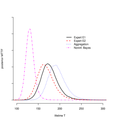
Figure 7: Posterior distributions of the MTTF for both experts and their aggregation, and in a noninformative framework.

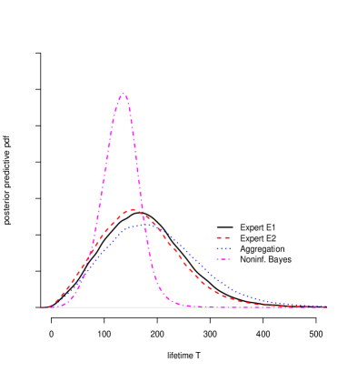
Figure 8: Posterior predictive densities for both experts and their aggregation, and in a noninformative framework.

4 Discussion

The elicitation of a multidimensional prior, perceived as a reference posterior conditional to virtual data supposed to reflect a perfect expert opinion, is a practical way of assessing indirectly the correlations in the parameter space, coherently with the sampling model. Another important gain is the possibility of assessing the prior uncertainty in an understandable way by modulating the virtual size, for instance for sensitivity studies. This indicator of prior information might help to increase the trust of a decision-maker in the posterior beliefs and the acceptation of Bayesian assessments by control authorities. Unfortunately, such priors are often untractable since they require to assess nonexhaustive statistics of the virtual data. This is especially the case with the Weibull models.

In this article, however, we showed how this issue can be overcome, replacing those untractable statistics with functionals such that the resulting prior answers to the statistical specifications of the prior knowledge, under the form of percentiles. Note that other alternatives to percentiles could have been considered: for instance, following Percy PER02 , assume an expert can provide an estimate $t_{e}$ of the marginal MTTF or the mode $\mbox{Md}[T]$, namely

$$\mbox{MTTF}\ =\ \mbox{E}[T] = \iint_{I\!\!R^{2}_{+}}\mbox{E}[T|\eta,\beta]f_{W}(t|\eta,\beta)\pi(\eta,\beta)\ d\eta d\beta,$$

$$\mbox{Md}[T] = \arg\limits_{t>0}\max\iint_{I\!\!R^{2}_{+}}f_{W}(t|\eta,\beta)\pi(\eta,\beta)\ d\eta d\beta.$$

The first estimate $t_{e}$ is thus related to a quadratic loss function $\Lambda(t_{0},t|c_{1},c_{2})$ which assumes the equality of costs $c_{1}=c_{2}$ and a penalisation increasing with $|t_{0}-t|$, while the second can be explained by the limit of a series of binary loss functions Robert, C.P. (2001). Following the principle described in Proposition 2.2, one should replace $b({\bf\tilde{t}_{m}},\beta)$ in (3) by, respectively (see Bousquet, N. (2006) for details),

$$b(m,\beta) = \left(\frac{\Gamma(m)}{\Gamma(1+1/\beta)\Gamma(m-1/\beta)}\right)^{\beta}t^{\beta}_{e},$$

$$b(m,\beta) = \left(\frac{m\beta+1}{\beta-1}\right)t^{\beta}_{e}.$$

However, $\pi(\beta)$ is no longer (but remains close to) a gamma density, and furthermore these two specifications require conditions over $m$ and the domain of variation of $\pi(\beta)$ to be usable. Indeed, one must guarantee $\beta_{0}>1$ to ensure $b(m,\beta)$ is well defined when $t_{e}$ is specified as a unique mode. This is coherent with the Weibull features, since the Weibull distribution has a unique positive mode if and only if $\beta>1$. As explained before, assuming aging is an equivalent prior constraint placed on the model.

Since assuming a prior predictive percentile can be provided by an oriented questioning, and fortunately leads to an explicit and versatile joint prior on Weibull parameters, we suggest Bayesian reliability analysts should favor, as much as possible, this kind of elicitation. This agrees with the vision historically promoted by Berger Berger, J.O. (chap. 3) and Percy PER02 , who considered that quantile-based approaches pose among best elicitation methods, the estimation of probabilities of localization in given areas being simpler for experts than the assessment of statistical moments.

Along the paper some remaining issues and limitations of the prior modelling have been evoked, which are now discussed as potential avenues for future researches. These researches, besides, will be dedicated to extend this methodology to other models which are often used in reliability studies, especially extreme value models whose links with Weibull distributions are well known.

It appears firstly that checking for the appropriateness of the Weibull model with respect to the virtual data is a crucial task, since it allows to reveal divergences between an expert opinion and the common sense of reliability practicioners when assuming the Weibull distribution for the lifetime of an industrial component submitted to aging. As the case for expert ${\cal{E}}_{1}$ illustrates, providing a small prior credibility interval can underlie unrealistic values for the Weibull parameters. This agrees with the well-known behavior of RRA experts of underestimating their self-uncertainty Lannoy, A. and Procaccia, H. (2001). Therefore we suggest that spreading the prior credibility orders such that a qualitative requirement is reached (e.g., $P_{\pi}(\beta<2)=0.5$) can give a more reasonnable summary of the real knowledge of $\Sigma$.

Another issue deals with the remaining uncertainty in expert opinion. In this article, we proposed a simple definition of the ratio of subjective and objective information based on virtual and real data sizes, understandable outside the community of statistics. It is clear however that information quantities updated through Bayesian inference are also strongly dependent on the possible conflicting issues between prior and real data, in the sense that both can favor regions of the sample and parameter spaces which are far from each other Evans, M., & Moshonov, H. (2006); Bousquet, N. (2008). Tools proposed in these two references should be carried out to check the internal coherency of the Bayesian model beforehand.

Besides, we did not consider here the remaining difficulties occuring when the expert can be suspected of bias, for instance because of motivational reasons Benson and Nichols (1982) or dependency within a group. Many other tools, based on test experiments, have been proposed in the literature in order to quantify those biases (e.g. Singpurwalla, N.D. and Song, M.S. (1986); Singpurwalla, N.D. (1988); Lannoy, A. and Procaccia, H. (2001)). However, in absence of supplementary information, we prefered respecting the summarized expert opinions the best we could in our case-study.

Thus, the case of dependent experts has not been treated in this paper, since it remains controversial in Bayesian statistics oha06b and probably deserves specific studies in the RRA area. Pursuing our view, two experts are dependent if they share virtual data from their past experience, or if a part of a virtual sample is produced dependently from the other sample. Dependency could then be introduced through a hierarchical mechanism of data production, in the spirit of the supra-Bayesian approaches promoted by Lindley Lindley (1983). This theme will also be considered in our next works.

In future studies, it will be necessary too to provide some calibration tools to take into account the expert uncertainty and bias. A first avenue can simply be to add a hierarchical level conditional to $m$. Indeed, we assumed here that the expert subjectivity mainly lies in the self-estimation of the costs associated with a reliability decision, and thus (using notations from $\S$ 2.3) in the estimation of sorted orders $\alpha_{1}<\ldots<\alpha_{p}$. Let us denote $\tilde{\alpha}_{1}<\ldots<\tilde{\alpha}_{p}$ these prior estimates. If we pursue the virtual size idea, it appears logical to consider the $\alpha_{i}$ as correlated random variables such that, a priori,

$$\alpha_{1},\alpha_{2}-\alpha_{1},\ldots,\alpha_{p}-\alpha_{p-1},1-\alpha_{p} \sim {\cal{D}}_{ir}\left(\nu_{1},\ldots,\nu_{p+1}\right)$$

with $\nu_{i}-1$ being the number of virtual “past” observations of the event $t_{\alpha_{i-1}}\leq T\leq t_{\alpha_{i}}$, which induces $\sum_{i=1}^{p+1}\nu_{i}=m+p+1$, the Dirichlet distribution appearing naturally from well-known conjugation properties. Imposing $\mbox{E}[\alpha_{i}-\alpha_{i-1}]=\tilde{\alpha}_{i}-\tilde{\alpha}_{i-1}$ leads to elicit

$$\nu_{i} = (m+p+1)\left(\tilde{\alpha}_{i}-\tilde{\alpha}_{i-1}\right).$$

The obvious correlation between prior estimates $\tilde{\alpha}_{i}$ threatens to underestimate the prior uncertainty of the $\alpha_{i}$, so that it appears more appropriate to help the expert providing conditional probabilities by answering to the following question: what is the risk $\alpha_{i}-\alpha_{i-1}$ for $\Sigma$ to break down before $t_{\alpha_{i}}$ knowing $\Sigma$ still runs after $t_{\alpha_{i-1}}$? Thus, the randomization of values $(\alpha_{1},\ldots,\alpha_{p})$ imposes indirectly a prior distribution $\pi(\widetilde{\beta}^{*}(m))$ rather than a single value, and consequently, $m$ should now be calibrated as the minimizer of the expected expert incoherency risk

$$m^{*} = \arg\min_{m\geq 0}\mbox{E}_{\pi(\widetilde{\beta}^{*}(m))}\left[{\cal{D}}_{m}\left(f^{*},f_{\pi\left(.|\widetilde{\beta}^{*}(m)\right)}\right)\right].$$

But this calibration remains in facts difficult to carry out, since the untractability of $\pi(\widetilde{\beta}^{*}(m))$ imposes a double Monte Carlo approximation coupled to an optimization strategy. Our next research will focus on simplifying this computational work.

Finally, we remind to the reader that other elicitation approaches of percentile orders are possible, mainly based on the establishement of expert preferences on a series of bettings such that $\alpha$ is not directly estimated but is progressively bounded oha06b . Such methods are robust with respect to perturbations of the often criticized expected utility criterion, since they can lead to results that are independent of the behavior of the expert face to his or her self-perception of the risk ABD00 . It thus should be worthy to adapt our modelling and the calibration aspects to this type of elicitation, which could lead to more cautious, credible statistical features of the prior modelling.

Appendix

Proof of Proposition 2.2.

Denote ${\displaystyle f_{m}(\beta)=\frac{\beta^{m-1}\ }{{\left(b_{\alpha}(m,\beta)\right)^{m}}}\ \exp\left(m\frac{\beta}{\beta({\bf\tilde{t}_{m}})}\right)}$ and ${\displaystyle g_{m}(\beta)=\left({1+{\frac{t^{\beta}_{\alpha}}{b_{\alpha}(m,\beta)}}}\right)^{-m}}.$ Then, renaming $b({\bf\tilde{t}_{m}},\beta)$ in $b_{\alpha}(m,\beta)$ in (3-4),

$$P_{\pi}(T\leq t_{\alpha}) = \iint_{I\!\!R_{+}\times I\!\!R_{+}}F_{W}(t_{\alpha}|\eta,\beta)\pi(\eta|\beta)\pi(\beta)\ d\eta d\beta,$$

$$= 1-{\displaystyle\Delta_{m}\left.\int_{I\!\!R_{+}}f_{m}(\beta)g_{m}(\beta)\ d\beta\right.}$$

where $\Delta^{-1}_{m}=\int_{I\!\!R_{+}}f_{m}(\beta)\ d\beta$ which must be necessarily finite to get a proper $\pi(\beta)$. Assuming $P_{\pi}(T\leq t_{\alpha})=\alpha$ leads to $\int_{I\!\!R_{+}}f_{m}(\beta)h_{m}(\beta)\ d\beta=0$ where $h_{m}(\beta)=g_{m}(\beta)-(1-\alpha)$ which is continuous in $\beta\geq 0$ if $\beta\mapsto b_{\alpha}(m,\beta)$ is assumed continuous for any $m>0$. Since $\beta\mapsto f_{m}(\beta)>0$ except possibly on a finite number of points in $I\!\!R_{+}$, $h_{m}(\beta)=0$ almost everywhere in $I\!\!R_{+}$. Expression (5) follows immediately.

Lemma 1. Denote ${\cal{M}}_{1}$ and ${\cal{M}}_{2}$ two sampling models with same parameter $\theta$. Denote ${\bf\tilde{t}_{m_{i}}}$ a non-observed ${\cal{M}}_{1}-$sample with likelihood ${\ell}_{{\cal{M}}^{(1)}}$. Let ${\bf\tilde{s}_{m_{i}}}=g({\bf\tilde{t}_{m_{i}}})$ be an observed ${\cal{M}}_{2}-$sample with likelihood ${\ell}_{{\cal{M}}^{(2)}}$, such that $\theta\mapsto{\ell}_{{\cal{M}}^{(2)}}(\theta)\propto{\ell}_{{\cal{M}}^{(1)}_{i}}(\theta)$. Denote $\pi^{J}$ a prior measure on $\theta$ and $\pi^{J}_{{\cal{M}}^{(j)}}$ its posterior knowing likelihood ${\ell}_{{\cal{M}}^{(j)}}$. Then for $p$ various samples ${\bf\tilde{t}_{m_{1}}},\ldots,{\bf\tilde{t}_{m_{p}}}$, one has

$$\pi^{J}_{{\cal{M}}^{(1)}}\left(\theta|{\bf\tilde{t}_{m_{1}}},\ldots,{\bf\tilde{t}_{m_{p}}}\right) = \pi^{J}_{{\cal{M}}^{(2)}}\left(\theta|{\bf\tilde{s}_{m_{1}}},\ldots,{\bf\tilde{s}_{m_{p}}}\right)$$

Proof.

The proof is straightforward, and we can consider only two non-observed samples ${\bf\tilde{t}_{m_{1}}}$ and ${\bf\tilde{t}_{m_{2}}}$ (corresponding possibly to two independent expert opinions). Then

$$\pi^{J}_{{\cal{M}}^{(1)}}\left(\theta|{\bf\tilde{t}_{m_{1}}},{\bf\tilde{t}_{m_{2}}}\right) \propto \ell_{{\cal{M}}^{(1)}}\left({\bf\tilde{t}_{m_{1}}}|\theta\right)\pi^{J}_{{\cal{M}}^{(1)}}\left(\theta|{\bf\tilde{t}_{m_{2}}}\right),$$

$$\propto \ell_{{\cal{M}}^{(2)}}\left({\bf\tilde{s}_{m_{1}}}|\theta\right)\pi^{J}(\theta)\ell_{{\cal{M}}^{(1)}}\left({\bf\tilde{t}_{m_{2}}}|\theta\right),$$

$$\propto \ell_{{\cal{M}}^{(2)}}\left({\bf\tilde{s}_{m_{1}}}|\theta\right)\ell_{{\cal{M}}^{(2)}}\left({\bf\tilde{s}_{m_{2}}}|\theta\right)\pi^{J}(\theta),$$

$$\propto \ell_{{\cal{M}}^{(2)}}\left({\bf\tilde{s}_{m_{1}}}|\theta\right)\pi^{J}_{{\cal{M}}^{(2)}}\left(\theta|{\bf\tilde{s}_{m_{2}}}\right),$$

$$\propto \pi^{J}_{{\cal{M}}^{(2)}}\left(\theta|{\bf\tilde{s}_{m_{1}}},{\bf\tilde{s}_{m_{2}}}\right)$$

and the equality follows by immediate normalization.

Proof of Proposition 2.4.

The Weibull likelihood of the $m$ virtual data summarized by $(t_{\alpha},\alpha,\widetilde{\beta}(m))$ is proportional to $\ell(\eta,\beta)=\pi(\eta,\beta)/\pi^{J}(\eta,\beta)$ where $\pi(\eta,\beta)$ is defined by (6-7). Modify the parametrization using $\mu=\eta^{-\beta}$. Thus

$$\ell(\mu,\beta) \propto \mu^{m}\exp\left(-\mu b_{\alpha}(m,\beta)\right)\beta^{m}\exp\left(-m\frac{\beta}{\widetilde{\beta}(m)}\right),$$

$$\propto \left[{\left\{\mu\left(t_{\alpha}\right)^{\beta}\right\}^{m}}\exp\left\{-\mu k_{\alpha,m}\left(t_{\alpha}\right)^{\beta}\right\}\right]\ \left[{\beta^{m}}\exp\left\{-m\frac{\beta}{\widetilde{\beta}(m)}\right\}\exp\left\{-m\beta\log t_{\alpha}\right\}\right],$$

$$\propto \ell_{1}\left(k_{\alpha,m}|\mu,\beta\right)\ \ell_{2}\left(\beta_{t_{\alpha},m}|\beta\right)$$

where

$$\ell_{1}\left(k_{\alpha,m}|\mu,\beta\right) \propto \frac{\left\{\mu\left(t_{\alpha}\right)^{\beta}\right\}^{m}}{\Gamma(m)}k^{m-1}_{\alpha,m}\exp\left\{-k_{\alpha,m}\left(t_{\alpha}\right)^{\beta}\right\}$$

which is the likelihood arising from considering $k_{\alpha,m}\sim{\cal{G}}(m,m\mu(t_{\alpha})^{\beta})$, and

$$\ell_{2}\left(\beta_{t_{\alpha},m}|\beta\right) \propto \frac{\left(m\beta\right)^{m}}{\Gamma(m)}\beta^{m-1}_{t_{\alpha},m}\exp\left\{-m\beta\frac{1+\widetilde{\beta}(m)\log t_{\alpha}}{\widetilde{\beta}(m)}\right\}$$

which is the likelihood arising from considering $\beta_{t_{\alpha},\delta}\sim{\cal{IG}}(m,m\beta)$.

References

- [1]
- [2] Abdellaoui, M. (2000). Parameter-free elicitation of utilities and probability weighting functions, Management Science, 46: 1497-1512.
- Bacha et al., [1998] Bacha, M., Celeux, G., Idée, E., Lannoy, A. and Vasseur, D. (1998). Estimation de modèles de durées de vie fortement censurées, Eyrolles (in French).
- Benson and Nichols [1982] Benson, P.G., and Nichols, M.L. (1982). An investigation of motivational bias in subjective predictive probability distribution. Decision Sci., 13: 10-59.
- [5] Berger, J.O. (1985). Statistical Decision Theory and Bayesian Analysis. Springer-Verlag, New York.
- Berger, J.O and Bernardo, J.M. [1992] Berger, J.O and Bernardo, J.M. (1992). On the development of reference priors (with discussion). In: J.M. Bernardo, J.O. Berger, A.P. Dawid and A.F.M. Smith, Eds., Bayesian Statistics 4, Oxford University Press: 35-60.
- Berger, J.O. and Sun, D. [1993] Berger, J.O. and Sun, D. (1993). Bayesian analysis for the Poly-Weibull Distribution, J. Amer. Statis. Assoc., 88: 1412-1418.
- [8] Bertholon, H., Bousquet, N., Celeux, G. (2006). An alternative competing risk model to the Weibull distribution in lifetime data analysis, Lifetime Data Analysis, 12: 481-504.
- Bousquet, N. [2006] Bousquet, N. (2006). A Bayesian analysis of industrial lifetime data with Weibull distributions, Research Report RR-6025, INRIA.
- Bousquet, N. [2008] Bousquet, N. (2006). Diagnostics of prior-data agreement in applied Bayesian analysis. J. Appl. Statist., 35: 1011-1029.
- [11] Brent, R. (1973). Algorithms for Minimization without Derivatives. Englewood Cliffs N.J.: Prentice-Hall.
- [12] Celeux, G., Marin, J.M., Robert, C.P. (2006). Sélection bayésienne de variables en régression linéaire. Journal de la Société Française de Statistique, 147: 59-79 (in French).
- [13] Clarke, B.S. (1996). Implications of reference priors for prior information and for sample size, J. Amer. Statis. Assoc., 91: 173-184.
- Cooke [1991] Cooke, R.M. (1991). Experts in Uncertainty: Opinion and Subjective Probability in Science. New York: Oxford University Press.
- [15] De Finetti, B. (1937). La prévision: ses lois logiques, ses sources subjectives. Annales de l’Institut Henri Poincaré (in French), 7: 1-68.
- [16] Dodson, B. (2006). The Weibull Analysis Handbook (2nd ed.). ASQ Quality Press, p. 7.
- [17] Efron, B. (1986). Why isn’t everyone a Bayesian? (with Discussion), The American Statistician, 40: 1-11.
- Evans, M., & Moshonov, H. [2006] Evans, M., & Moshonov, H. (2006). Checking for prior-data conflict. Bayesian analysis, 1: 893-914.
- [19] Gilks, W.R., Wild, P. (1992). Adaptive rejection sampling for Gibbs sampling. Applied Statistics, 41: 337-348.
- [20] Kadane, J.B., Wolfson, J.A. (1998). Experiences in elicitation, The Statistician, 47: 3-19.
- Kaminskiy, M.P., and Krivtsov, V.V. [2005] Kaminskiy, M.P., and Krivtsov, V.V. (2005). A Simple Procedure for Bayesian Estimation of the Weibull Distribution, IEEE Trans. Reliability, 54: 612-616.
- Kárny et al. [2003] Kárný, M., Nedoma, P., Khailova, N., Pavelková, L. (2003). Prior information in structure estimation. IEEE Proceedings in Control Theory and Applications, 150: 643-653.
- Kontkanen et al. [1998] Kontkanen, P., Myllymäki, P., Silander, T., Tirri, H., Grünwald, P. (1998). Bayesian and information-theoretic priors for Bayesian networks parameters. Lecture notes in computer science. In the proceedings of the ECML-98 European conference on machine learning, Chemnitz, Germany, 1398: 89-94.
- Lannoy, A. and Procaccia, H. [2001] Lannoy, A. and Procaccia, H. (2001). L’utilisation du jugement d’expert en sûreté de fonctionnement, Tec & Doc (in French).
- [25] Liang, F., Paulo, R., Molina, G., Clyde, M., Berger, J. (2008). Mixtures of g-priors for Bayesian variable selection. J. American Statist. Assoc., 103: 410-423.
- Lin, X., Pittman, J. and Clarke, B. [2007] Lin, X., Pittman, J. and Clarke, B. (2007). Information Conversion, Effective Samples, and Parameter Size. IEEE Trans. Info. Theory, 53: 4438-4456.
- Lindley [1983] Lindley, D.V. (1983). Reconciliation of probability distributions. Operations Research, 31: 866-880.
- [28] Marin, J.M., Robert, C.P. (2010). Les bases de la statistique bayésienne. Rapport des Universités Montpellier II & Dauphine - CREST (in French).
- Morita et al. [2007] Morita, S., Thall, P.F. and Mueller, P. (2007). Determining the effective sample size of a parametric prior. UT MD Anderson Cancer Center Department of Biostatistics, Working Paper Series. Working Paper 36.
- Neal [2001] Neal, R.M. (2001). Transferring prior information between models using imaginary data. Technical Report 0108, Dept. Statistics, Univ. Toronto.
- [31] O’Hagan, A., Buck, C. E., Daneshkhah, A., Eiser, J. R., Garthwaite, P. H., Jenkinson, D. J., Oakley, J. E., Rakow, T. (2006), Uncertain Judgements: Eliciting Expert Probabilities. John Wiley and Sons, Chichester.
- [32] Percy, D.F. (2003). Subjective Reliability Analysis Using Predictive Elicitation. In: Mathematical and Statistical Methods in Reliability, B.H. Lindqvist & K.A. Doksum (eds). Quality, Reliability & Engineering Statistics 7, World Scientific Publishing Co.: Singapore, pp. 57-72.
- [33] Press, S.J. (2003). Subjective and Objective Bayesian Statistics (second edition), New York: Wiley.
- Robert, C.P. [2001] Robert, C.P. (2001). The Bayesian Choice. A Decision-Theoretic Motivation (second edition), Springer.
- Singpurwalla, N.D. and Song, M.S. [1986] Singpurwalla, N.D. and Song, M.S. (1986). An analysis of Weibull lifetime data incorporating expert opinion, in Probability and Bayesian Statistics (R.Viertl ed.), Plenum Pub.Corp.: 431-442.
- Singpurwalla, N.D. [1988] Singpurwalla, N.D. (1988). An interactive PC-Based procedure for reliability assessment incorporating expert opinion and survival data, J. Amer. Statis. Assoc., 83: 43-51.
- Soland, R. [1969] Soland, R. (1969). Bayesian analysis of the Weibull process with unknown scale and shape parameters, IEEE Transactions on Reliability, 18: 181-184.
- Sun [1997] Sun, D. (1997). A note on noninformative priors for Weibull distributions, J. Statist. Planning and Inference, 61: 319-338.
- Sun and Speckman [2005] Sun, D., Speckman, P.L. (2005). A note on the nonexistence of posterior moments, Can. J. Statist., 33: 591-601.
- Tsionas, [2000] Tsionas, E.G. (2000). Posterior analysis, prediction and reliability in three-parameter Weibull distributions, Commun. Statist. - Theory Meth., 29(7): 1435-1449.
- Tsionas [2002] Tsionas, E.G. (2002). Bayesian analysis of finite mixtures of distributions, Commun. Statist. - Theory Meth., 31(1): 37-48.
- [42] Tversky, A., Kahneman, D. (1974). Judgment under Uncertainty: Heuristics and Biases, Science, 185: 1124-1131.
- [43] Unwin, S.D., Cazzoli, E.G., Davis, R.E., Khatib-Rahbar, M., Lee, M., Nourbakhsh, H., Park, C.K., Schmidt, E. (1989). An information-theoretic basis for uncertainty analysis: application to the QUASAR severe accident study, Reliability Engineering & System Safety, 26: 143-162.
- Zellner, A. [1986] Zellner, A. (1986). On assessing Prior Distributions and Bayesian Regression analysis with g-prior distribution regression using Bayesian variable selection, In Bayesian inference and decision techniques : Essays in Honor of Bruno De Finetti: 233-243, North-Holland, Elsevier.