Exciton Hierarchies in Gapped Carbon Nanotubes

Abstract

We present evidence that the strong electron-electron interactions in gapped carbon nanotubes lead to finite hierarchies of excitons within a given nanotube subband. We study these hierarchies by employing a field theoretic reduction of the gapped carbon nanotube permitting electron-electron interactions to be treated exactly. We analyze this reduction by employing a Wilsonian-like numerical renormalization group. We are so able to determine the gap ratios of the one-photon excitons as a function of the effective strength of interactions. We also determine within the same subband the gaps of the two-photon excitons, the single particle gaps, as well as a subset of the dark excitons. The strong electron-electron interactions in addition lead to strongly renormalized dispersion relations where the consequences of spin-charge separation can be readily observed.

Gapped carbon nanotubes are the subject of intense experimental jim ; flu ; rmp ; wang ; torrens ; lin and theoretical interest ogawa ; axial ; levtsv ; louie ; vasily ; kane ; vasily1 ; molinari ; louie1 ; smitha ; egger due to their possible application as opto-electronic devices jim as well as providing a particularly clean realization of strongly correlated electron physics in low dimensions levtsv ; egger . Both interests converge in the study of the tubes’ excitonic spectra. This spectra, due to the effects of a strong Coulomb interaction in one dimension, is strongly renormalized from what would be expected from the underlying band structure of the tube. Its computation therefore requires a non-perturbative approach.

The favoured theoretical approach to studying the excitonic spectra of carbon nanotubes is the use of a Bethe-Salpeter equation combined with first principle input to approximate the particle and hole wavefunctions that form the excitons louie ; vasily ; vasily1 ; louie1 . This approach has been particularly valuable in that it has allowed a quantitative description of aspects of excitonic physics, in particular the magnitude of the excitonic gap for the lowest lying excitons in a given subband of the nanotube. In this letter we step away from trying to describe quantitative details of the excitons and instead focus on more qualitative features. We do so using an approach that combines a field theoretic reduction of the nanotubes identical to that used to study Luttinger liquid behaviour in metallic nanotubes with a numerical renormalization group that enables one to study the effects of gapping out a multi-component Luttinger liquid. In the process we find in a regime of strong electron-electron interactions a number of new qualitative features to the excitonic spectra (see Fig. 1).

First and foremost we find that a given subband of the nanotube has a finite number of optically active one-photon excitons, $\Delta^{1u,i}$, where the multiplicity depends on the strength of the tube’s screened Coulomb interaction. While a simple picture of excitons as analogs of the excited states of a hydrogen atom ogawa yields an infinite hierarchy of excitons, we argue this series is truncated to at most three. In order to understand the excitons’ binding energy, we also study the single particle spectrum of the tube. The single particle gap is strongly renormalized by interactions and can be many multiples of the bare bandgap. Consequently the lowest lying two-excitation continuum, depending on strength of the Coulomb interaction, may be a particle-hole continuum or it may be a two-exciton continuum. This approach treats all excitations of the nanotube on the same footing. It thus conflates the difference between an exciton and a bi-exciton. Indeed interactions can be sufficiently strong that excitons should then be thought of equally as particle-hole bound states or bound states of two other excitons.

Figure 1: A schematic indicating the position in energy of the various excitons together with two-excitation continua arising from our treatment at larger values of the effective interaction ($K_{c+}^{-1}\geq 5$). The bracketed numbers are estimates computed at $K_{c+}=1/7$ of the relative absorption strength (relative to the strength of $\Delta^{1u,1}$) of the three one-photon optically active excitons, $\Delta^{1u,1-3}$.

Our results are applicable both to semiconducting nanotubes and metallic nanotubes which have been turned semiconducting by the application of an axial magnetic field axial . In the latter case where the gap is tunable and can be made much smaller than the bandwidth, we expect our approach to yield results that are quantitatively accurate. For tubes that are semiconducting due to band structure, our results within a one subband approximation are most reliable for large radius tubes although we believe the qualitative features that we find to apply equally well to smaller radius tubes.

We focus on a single subband of a carbon nanotube. To describe this subband at low energies we introduce four sets (two for the spin, $\sigma$, degeneracy and two for the valley, $\alpha=K,K^{\prime}$, degeneracy) of right ($r=+$) and left ($r=-$) moving fermions, $\psi_{r\alpha\sigma}$. The Hamiltonian governing these fermions can be written as $H=\int dx(H_{kin}+H_{gap})+H_{Coulomb}$. $H_{kin}+H_{gap}$ together give the non-interacting band dispersion, $\epsilon^{2}(p)=v_{0}^{2}p^{2}+\Delta_{0}^{2}$:

$$H_{kin}=-iv_{0}\psi^{\dagger}_{r\alpha\sigma}\partial_{x}\psi_{r\alpha\sigma};~{}~{}H_{gap}=\Delta_{0}\psi^{\dagger}_{r\alpha\sigma}\psi_{-r\alpha\sigma},$$ (1)

where $v_{0}$ is the bare velocity of the fermions and repeated indices are summed. For the Coulombic part of the Hamiltonian we include only the strongest part of forward scattering:

$$H_{Coulomb}=\frac{1}{2}\int dxdx^{\prime}\rho(x)V_{0}(x-x^{\prime})\rho(x^{\prime}),$$

where $\rho(x)=\sum_{r\alpha\sigma}\psi^{\dagger}_{r\alpha\sigma}(x)\psi_{r\alpha\sigma}(x)$. We also ignore backscattering interactions arising from Coulomb interactions. In the presence of a gap term, these interactions, as they are marginal in the RG sense, are less important. But as they lift the model’s SU(4) symmetry, they will split the lowest lying 15-fold multiplet of optically dark excitons.

To study the full Hamiltonian, we treat $H_{gap}$ as a perturbing term (albeit one to be treated non-perturbatively) of $H_{0}\equiv\int dx(H_{kin})+H_{Coulomb}$. The latter terms are nothing more than the Hamiltonian of a metallic carbon nanotube. In excitonic language, we thus think of $H_{gap}$ as a confining interaction on top of the metallic tube. The advantage of doing so is that we are able to treat Coulomb interactions analytically exactly at the beginning of the computation. We do so using bosonization.

If we bosonize $H_{0}$ in terms of chiral bosons $\phi_{r\alpha\sigma}$ by writing $\psi_{r\alpha\sigma}\sim\exp(i\phi_{r\alpha\sigma})$, we arrive at a simple result kane1 ; egger . The theory is equivalent to four Luttinger liquids described by the four bosons $\theta_{i}$, $i=c_{\pm},s_{\pm}$ (and their duals $\phi_{i}$)

$$H_{0}=\int dx\sum_{i}\frac{v_{i}}{2}\bigg{(}K_{i}(\partial_{x}\phi_{i})^{2}+K_{i}^{-1}(\partial_{x}\theta_{i})^{2}\bigg{)}.$$ (2)

The four bosons diagonalizing $H_{0}$ are linear combinations of the original four bosons and represent an effective charge-flavour separation where $\theta_{c+}=\sum_{r\alpha\sigma}r\tilde{\psi}_{r\alpha\sigma}$ is the charge boson and the remaining three bosons reflect the spin, valley, and parity symmetries in the problem. The charge boson is the only boson to see the effects of the Coulomb interaction. Both the charge Luttinger parameter $K_{c+}$ and the charge velocity $v_{c+}=v_{0}/K_{c+}$ are strongly renormalized. In particular for long range Coulomb interactions, $K_{c+}$ takes the form

$$K_{c+}=\bigg{(}1+\frac{8e^{2}}{\pi\kappa\hbar v_{0}}\big{(}\log(\frac{L}{2\pi R})+c_{0}\big{)}\bigg{)}^{-1/2},$$ (3)

where $\kappa$ is the dielectric constant of the substrate, $L$ is the length of the nanotube, $R$ is the tube’s radius, and $c_{0}$ is an $O(1)$ numerical constant dependent on details of the wrapping vector $(n,m)$ smitha ; egger . In typical nanotubes $K_{c+}$ can take on values in the range of $\sim.2$. With an electric field applied transversely to the tube, $K_{c+}$ can easily be made as small as $.1$ smitha . The remaining Luttinger parameters, $K_{i}$, $i=c_{-},s_{\pm}$ retain their non-interacting values, $1$, and so their velocities, $v_{i}=v_{0}$ go unrenormalized. Including the full forward scattering leads to a small (upwards) renormalization (on the order of 10%) of these parameters which we will not consider here egger . These renormalizations, however, will not change any of our results qualitatively.

Under bosonization, $H_{gap}$ becomes

$$H_{gap}=\frac{4\tilde{\Delta}_{0}}{\pi}(\prod_{i}\cos(\frac{\theta_{i}}{2})+\prod_{i}\sin(\frac{\theta_{i}}{2})),$$ (4)

where $\tilde{\Delta}_{0}=\Delta_{0}(\Lambda/v_{c+})^{(1-K_{c+})/4}$ and $\Lambda$ is the bandwidth of the tube. This gap term is highly relevant. Rewriting the gap term in this fashion already gives us important generic features of the excitonic spectrum. Firstly, as a perturbation of $H_{0}$, $H_{gap}$ has the anomalous dimension, $3/4+K_{c+}/4$. In turn this implies the full gaps, $\{\Delta_{\alpha}\}_{\alpha}$, satisfy the scaling relation

$$\Delta_{\alpha}=\Lambda(\frac{\Delta_{0}}{\Lambda})^{4/(5-K_{c_{+}})}f_{\alpha}(K_{c+})$$ (5)

where $\{f_{\alpha}\}_{\alpha}$ is a set of a priori unknown dimensionless functions of $K_{c+}$. We will see that for the excitons, $f_{Exc}$ is a relatively weak function of $K_{c+}$ while for the single particle excitations, $f_{sp}$ depends strongly on $K_{c+}$. This scaling relation tells us immediately how exciton gaps scale between subbands. If we take a large radius tube where the gap of the n-th subband gaps scale as $\Delta_{0}(n,R)\sim n/R$, the expected gap ratio between the first and second subband, is $2^{4/(5-K_{c+})}\sim 1.78$ (this is in rough correspondence to that reported in flu and so provides a straightforward explanation of the ratio problem kane ). Secondly, $H_{gap}$ takes the form of a perturbation of a generalized sine-Gordon model (involving four bosons instead of one). We thus expect that excitons (within a given subband) will come in hierarchies whose size is determined by the value of $K_{c+}$ very much like the number of bound states in a sine-Gordon model, a perturbation on a free boson of the form $\cos(\beta\theta)$, is determined by the parameter $\beta$.

Having completely characterized $H_{0}$, we study the confining effects of $H_{gap}$ using the truncated conformal spectrum approach (TCSA) zamo combined with a Wilsonian renormalization group modeled after the numerical renormalization group (NRG) used to study quantum impurity problems kon1 . This methodology permits the study of arbitrary continuum one dimensional theories provided one can write the theory as the sum of a gapless theory, in this case $H_{0}$, plus a perturbation, here $H_{gap}$. It is flexible enough that it can play the same role as DMRG does for lattice models (although as it is an NRG, it accesses matrix elements more easily). Among the first uses of the original TCSA, unequipped with an NRG, was to study a quantum Ising model in a magnetic field zamo . The model we study here, in terms of computational complexity, is equivalent to eight coupled Ising models. Because of this added complexity, this model could not be studied using the TCSA without the accompanying renormalization group. Additional details of this approach as applied to the problem at hand may be found in Section I of Ref. epaps .

Our results for the gaps as a function of $K_{c+}$ are presented in Fig. 2. Details of the analysis of the numerical data have also been relegated to Ref. epaps . We emphasize again that these excitations are all found within a single subband of the tube. We first consider the one-photon optically active excitons (labelled $\Delta^{1u,i}$, $i=1,2,3$ where here $u$ refers to the antisymmetry under $\pi-$rotations about the centre of a carbon hexagon – in bosonic language antisymmetry under this rotation corresponds to antisymmetry under $\theta_{c+,s+}\rightarrow-\theta_{c+,s+}$). We see that as $K_{c+}$ decreases (i.e. the effective Coulomb interactions become stronger) the number of one photon excitons grows. At $K_{c+}\geq 1/5$ the number of such excitons goes from one to two, while at $K_{c+}\geq 1/6$ the number of such excitons goes from two to three. But thereafter this number saturates.

There are two limits on stable excitons in the system – the beginnings of both the particle-hole continuum (marked in dark green in Fig. 2) and a two-exciton continuum (marked in maroon in Fig. 2). Necessarily exciton gaps cannot cross over these boundaries lest a decay channel opens to the exciton. The bottom of the particle-hole continuum is twice the single particle gap, $2\Delta^{sp}$. As $\Delta^{sp}$ is a strong function of $K_{c+}$ (going as $\Delta^{sp}\sim K_{c+}^{-1}$), at small $K_{c+}$ there is room for additional excitons. This is very much like the sine-Gordon model where as $\beta$ goes to zero, the number of bound states goes to infinity. However for an exciton to be stable it must also fall below a two-exciton continuum. This two-exciton continuum, formed from the lowest single-photon exciton, $\Delta^{1u,1}$, and the lowest two-photon exciton, $\Delta^{2g,1}$, is relatively insensitive to $K_{c+}$ and serves to provide a bound on the total number of possible excitons at small $K_{c+}$.

Figure 2: The exciton and single particle energies as a function of $K_{c+}$.

In bosonized models considerable intuition can be had by considering the classical limit and asking what are the classical field solutions that correspond to the excitons/bound states. This is true here as well. The first one-photon exciton, $\Delta^{1u,i}$, corresponds to a breather-like solution of the field equations governing $H_{0}+H_{gap}$. This solution corresponds to $\theta_{c+}$ interpolating between $0$ to $4\pi$ and back to $0$ while the other three bosons remain fixed at $0$. It takes the form

$$\theta_{c+}(x,t)=4\tan^{-1}\frac{\sqrt{1-\omega^{2}}\cos(\omega t)}{\omega\cosh(\sqrt{1-\omega^{2}}x)},$$ (6)

where $\omega$ is related to the (classical) energy of the breather. We can estimate the energy corresponding to quantizing this classical solution via mean field theory. Replacing $H_{gap}$ by $4\tilde{\Delta}_{0}/\pi\Xi^{3}\cos(\theta_{c+}/2)$, where $\Xi\equiv\langle\cos(\theta_{f}/2)\rangle$ with $\theta_{f}=\theta_{c-},\theta_{s+}$, or $\theta_{s-}$, we reduce the model to a pure sine-Gordon theory. $\Delta^{1u,1}$ is then equal to the gap of this theory’s first bound state zamo1

$$\Delta^{1u,1}_{MFT}=2\big{(}2\tilde{\Delta}_{0}\Xi^{3}\frac{\Gamma(1-\frac{\alpha}{2})}{v_{c+}^{\alpha-1}\Gamma(\frac{\alpha}{2})}\big{)}^{\frac{1}{2-\alpha}}\frac{2\Gamma(\frac{\xi}{2})\sin(\frac{\pi\xi}{2})}{\sqrt{\pi}\Gamma(\frac{1}{2}+\xi)},$$ (7)

where $\alpha=1/4K_{c+}^{2}$ and $\xi=\alpha/(2-\alpha)$. $\Xi$ is determined self-consistently by replacing $H_{gap}$ with $4\tilde{\Delta}_{0}\pi^{-1}\Xi^{2}\langle\cos(\theta_{c+}/2)\rangle\cos(\theta_{f}/2)$ and using luk to express $\Xi$ in terms of the effective coupling constant $4\tilde{\Delta}_{0}\pi^{-1}\Xi^{2}\langle\cos(\theta_{c+}/2)\rangle$. We consequently find that as $K_{c+}^{-1}$ varies between $2$ and $10$, $\Delta^{1u,1}_{MFT}/(\Lambda(\Delta_{0}/\Lambda)^{4/(5-K_{c+})})$ varies from $3.1$ to $4.1$ in reasonable agreement (if shifted upwards) with the non-perturbative NRG.

The second one-photon exciton, $\Delta^{1u,2}$, has a gap a little more than twice that of $\Delta^{1u,1}$ and corresponds to roughly the putative location of $\Delta^{2u,1}$, the first exciton in the second subband (which we have argued, by scaling, is found at $\sim 1.8\Delta^{1u,1}$). If we were to take into account intersubband Coulomb interactions, hitherto ignored, $\Delta^{1u,2}$ and $\Delta^{2u,1}$ would mix leading to a set of hybridized states. It is thus conceivable that reports of observations of the exciton $\Delta^{2u,1}$ are in fact seeing $\Delta^{1u,2}$ or at least some hybridized combination of the two.

Beyond the one-photon excitons, Fig. 2 also displays the gaps of a number of other excitons. It shows the single existing two-photon exciton, $\Delta^{2g,1}$ (here g corresponds to excitons which are symmetrical under $\pi$-rotations about a centre of a carbon hexagon). Unlike the one-photon excitons, there is only a single stable two-photon exciton regardless of the value of $K_{c+}$. Lying just below $\Delta^{1u,1}$ are found a set of 15 dark excitons with energy $\Delta^{dark}$. These excitons subsume the dark triplet excitons but are of greater degeneracy because they not only carry spin quantum numbers but valley quantum numbers as well (dark excitons with non-trivial valley quantum number were termed $K$-momentum excitons in Ref. torrens ). As the full symmetry of $H$ is SU(4), the dark excitons transform as SU(4)’s adjoint. At twice the energy of $\Delta^{dark}$ begins a two exciton continuum into which any two-photon exciton will decay. As $\Delta^{2g,1}$ is just below $2\Delta^{dark}$, we understand this two exciton continuum essentially precludes any two-photon excitons with energy greater than $\Delta^{2g,1}$.

Figure 3: The dispersion of the first two excitons $\Delta^{1u,1}$ and $\Delta^{1u,2}$ for $K_{c+}=1/5$. Dashed lines in the small, but finite, momentum regions connecting data points are guides to the eye.

By examining the momentum dependence of the excitons’ dispersions, we can see the consequences of having two velocities, charge, $v_{c+}$, and flavour $v_{0}=v_{c-},v_{s\pm}$, in the system. The above semiclassics suggests that the initial dispersion of $\Delta^{1u,1}$, $E^{1u,1}(p)$, will behave approximately as $((\Delta^{1u,1})^{2}+p^{2}v_{c+}^{2})^{1/2}$ (a consequence of it involving $\theta_{c+}$ degrees of freedom alone). While we cannot write down the classical solution corresponding to $\Delta^{1u,2}$, it lies primarily in the spin/flavor sector and so will disperse governed by the much smaller velocity, $v_{0}$. While $\Delta^{1u,2}>\Delta^{1u,1}$, the much larger charge velocity means that the dispersion of $\Delta^{1u,1}$ will intersect $\Delta^{1u,2}$ at a relatively small momentum, $p_{int}=(((\Delta^{1u,2})^{2}-(\Delta^{1u,1})^{2})/(v_{c+}^{2}-v_{0}^{2}))^{1/2}$. This intersection means the two states will hybridize. As a consequence of this hybridization, for momenta larger than $p_{int}$, $\Delta^{1u,1}(p>p_{int})$ will disperse with an effective mass determined by $v_{0}$ whereas $\Delta^{1u,2}(p>p_{int})$ will now vary according to a velocity much closer to the larger $v_{c+}$.

We observe this general behaviour in our numerical analysis. Plotted in Fig. 3 are the dispersions of these two excitons for $K_{c+}^{-1}=5$. We see that $E^{1u,1}(p)$ increases extremely rapidly for momenta up to $p\sim\Delta/2v_{0}$ but thereafter levels out, even decreasing. This increase is greater than would be predicted from the relativistic dispersion, $((\Delta^{1u,1})^{2}+p^{2}v_{c+}^{2})^{1/2}$, suggesting that charge and spin, even at the smallest momenta, are intricately linked, leading to an even stronger renormalization of the effective mass. If however we combine the renormalization due to $v_{c+}$ with the logarithmic correction $p^{2}log(p)$, to the exciton self-energy predicted in Refs. kane ; vasily1 , we can understand the observed behaviour. Complementarily, $E^{1u,2}(p)$ initially displays a weak momentum dependence but then increases with a velocity approximately $v_{c+}/2$ for $p>p_{int}$.

Finally we touch upon the excitonic signal in absorption spectra. The strength of this signal is proportional to the imaginary part of the current-current correlator. It is straightforward to compute the necessary matrix elements of the current operator within the framework of TCSA+NRG. We find, as indicated in Fig. 1, that $\Delta^{1u,1}$ has by far the strongest signal. While $\Delta^{1u,2}$ should be visible in an absorption spectra, $\Delta^{1u,3}$, with a weighting 1/1000 of $\Delta^{1u,1}$ is effectively dark although could be detected indirectly through its effects on the temperature dependence of the excitonic radiative lifetime vasily1 .

In conclusion, we have argued for, using a fully many-body, non-perturbative approach, new features in the excitonic spectrum of gapped carbon nanotubes. We have shown that with a given subband, optically active excitons appear in finite hierarchies. We have also shown that the single particle sector experiences extremely strong renormalization so swapping the beginning of the particle-hole continuum with the two-exciton continuum. Further work will include studying the effects of backscattering interactions in the tubes (not treated here) together with intersubband interactions. More generally, we have demonstrated a robust method able to treat continuum representations of arbitrary one-dimensional systems.

RMK acknowledges support from the US DOE (DE-AC02-98 CH 10886) together with helpful discussions with V. Perebeinos, M. Sfeir, and A. Tsvelik.

I Supplementary Material: Exciton Hierarchies in Gapped Carbon Nanotubes

I.1 Description of NRG treatment of TSA as applied to gapped carbon nanotubes

We study the confining effects of $H_{gap}$ using the truncated conformal spectrum approach. As orginally developed zamo , the TCSA has been used extensively (for a sample consider lassig ; klas_mel ; takacs ; fioravanti ; takacs1 ; takacs2 ; lepori ). However here we combine it with a Wilsonian renormalization group modeled after the numerical renormalization group (NRG) used to study quantum impurity problems kon1 . With quantum impurity problems, the NRG exploits the idea that sites on the Kondo lattice far away from the quantum impurity are less important than sites close to the impurity in determining the physics. We have a similar notion here as the perturbation $H_{gap}$ is relevant in the RG sense (the anomalous dimension of the operator, $3/4+K_{c+}/4$, is less than 2) and so the eigenstates of the unperturbed Hamiltonian, $H_{0}$, lowest in energy are most important in determining the physics of the full model. We are thus justified in initially truncating the spectrum of $H_{0}=\int dx(H_{kin})+H_{Coulomb}$ to a finite number of states (for the computations chosen here, we initially truncate at $2500$). To be able to do so, we study the theory at finite size, $R_{NRG}$. In making the system finite, the spectrum becomes discrete with level spacing $2\pi/R_{NRG}$. However even at finite size, the conformal nature of $H_{0}$ means we have complete control over the spectrum (which can be thought of as a four-fold tensor product of states coming from Hilbert spaces of compactified bosons).

The Hilbert space of the theory can be described more properly as follows. For a single boson, with compactification radius, R, the Hilbert space is built from a set of highest weight states denoted by $|n,m\rangle$ where $n$ gives the center of mass momentum, $n/R$, of the state, and $m$ denotes the winding number (or charge) of the state diF . $|n,m\rangle$ is related to the true vacuum state, $|0\rangle$, by

$$|n,m\rangle=e^{\frac{in}{R}\theta(0)+\frac{imR}{2}\phi(0)}|0\rangle,$$

where $\phi$ is the boson dual to $\theta$. Descendant states may be created by acting on the $|n,m\rangle$ with a set of oscillator modes $a_{-n}$, $\bar{a}_{-n}$, $n>0$, that come from mode expanding the boson. For our multibosonic system with bosons, $\theta_{c\pm}$, $\theta_{s\pm}$, the set of highest weight states are formed according to

$$|n_{i};m_{i}\rangle = e^{i\sum_{j}\frac{n_{j}\sqrt{K_{j}}}{2}\theta_{j}(0)+i\sum_{j}\frac{m_{j}}{4\sqrt{K_{j}}}\phi_{j}(0)}|0\rangle;$$ (8)

$$\sum_{i}n_{i}~{}{\rm mod}~{}4 = 0;~{}~{}~{}\sum_{i}m_{i}~{}{\rm mod}~{}4=0;$$ (10)

$$\hskip-36.135pt\sum_{i}n_{i}m_{i}~{}{\rm mod}~{}4=0;$$

$$(n_{i}+n_{i+1})~{}{\rm mod}~{}2 = 0;~{}~{}~{}(m_{i}+m_{i+1})~{}{\rm mod}~{}2=0.$$ (11)

These particular conditions upon the highest weight states may be derived by considering the original bosons that arise in bosonizing the subband fermions (i.e. before the transformation to the charge and spin bosons). Descendant states are again formed by acting on these states with the modes $a_{i,-n}$, $\bar{a}_{i,-n}$, $n>0$, of the bosons. We note that we can show this Hilbert space leads to a modular invariant partition function indicating we have a well defined theory diF . The action of $H_{0}$ upon a state of the form

$$|E^{0}\rangle=\prod^{4}_{j=1}(a_{j,-k_{j1}}a_{j,-k_{j2}}\cdots a_{j,-k_{jN_{j}}})|n_{i},m_{i}\rangle$$

is

$$H_{0}|E^{0}\rangle = \frac{2\pi}{R_{NRG}}\bigg{(}\sum_{j}v_{j}(\frac{K_{j}n_{j}^{2}}{4}+\frac{m_{j}^{2}}{16K_{j}}-1/12)$$ (13)

$$+\sum_{j}v_{j}(\sum^{N_{j}}_{l=1}k_{jl})\bigg{)}|E^{0}\rangle,$$

where the $K_{j}$ are the four Luttinger parameters.

Having described the Hilbert space, we now label the discretized spectrum, $|E^{0}_{1}\rangle,|E^{0}_{2}\rangle,\cdots$ where the spectrum has been ordered in terms of increasing energy. We then truncate the spectrum keeping the first $N+\Delta$ states of the unperturbed theory, $|E^{0}_{1}\rangle,\cdots,|E^{0}_{N+\Delta}\rangle$ (where $N=1500$ and $\Delta=1000$ were typically chosen for this study). We further exploit our control over the unperturbed theory by computing all the matrix elements of $H_{gap}$, i.e. $\langle E^{0}_{i}|H_{gap}|E^{0}_{j}\rangle$. This knowledge then allows us to represent the full Hamiltonian as a $(N+\Delta)\times(N+\Delta)$ matrix which we then diagonalize. If $H_{0}$ were a simple theory, this procedure would be enough to obtain highly accurate results. In studying the critical transverse field Ising model perturbed by a parallel magnetic field, Ref. zamo, was able to keep only 39 states and yet still obtain the spectrum of the theory to an accuracy of a few percent. However a single Luttinger liquid can roughly be thought of (in terms of complexity of the Hilbert space) as a tensor product of two Ising models. Thus $H_{kin}+H_{Coulomb}$, being composed of four bosons, can be thought of as equivalent in complexity to a tensor product of eight Ising models. This eight fold complexity means that a simple truncation can no longer hope to describe correctly the physics. This is where the numerical renormalization group (NRG) is crucial, which we now briefly describe.

The NRG begins by taking the states arising from the diagonalization of the $(N+\Delta)\times(N+\Delta)$ matrix and ordering them in terms of increasing energy, $|E^{1}_{1}\rangle,\cdots,|E^{1}_{N+\Delta}\rangle$. We then discard the top $\Delta$ states. We re-form the truncated Hilbert space by taking the lowest $N$ energy states remaining from the diagonalization and add to them the next $\Delta$ states from the unperturbed spectrum. We thus obtain a truncated Hilbert space of the same size ($N+\Delta$): $|E^{1}_{1}\rangle,\cdots,|E^{1}_{N}\rangle,|E^{0}_{N+\Delta+1}\rangle,\cdots,|E^{0}_{N+2\Delta}\rangle$. We re-form the Hamiltonian in this new basis, rediagonalize, and then repeat the procedure until convergence. In this way, we allow the high energy portion of the unperturbed spectrum to influence the low energy sector in bite size, numerically manageable ($\Delta$) chunks.

In our study of the exciton gaps, we typically iterate the NRG up to 70 times (and so with a $\Delta=1000$, we take into account  $70000$ states of the unperturbed theory). While the results are not completely converged, we allow an analytic RG to take over from the numerical RG. At sufficiently high energies, the flow of a gap under the RG is governed by a simple one loop equation kon1 . We can thus fit the flow equation to our numerical data at high truncation energies and extrapolate to infinite truncation energy. For single particle gaps however, we found we needed to iterate the NRG many more times than for the excitons. Because of the large charge velocity (at least at small values of $K_{c+}$), we needed to take into account on the order of 1200000 states from the unperturbed theory. If we were to use the NRG as described in Ref. kon1 , this would mean iterating the NRG over 1000 times, a too great of numerical burden (the computational time scales as the number of iterations to the third power). We have thus adapted the NRG in this case. The great majority of the 1200000 states that the NRG needs to run through in the single particle case do not influence the end result. We thus run a ’preselection’ of the most important states and run the NRG on those. This works straightforwardly as follows.

To run the preselection, we run the NRG as initially described for M iterations (and so account for the first $N+M\Delta$ states of the unperturbed theory). We have then obtained a reasonable approximate (though not yet fully converged) of the lowest lying eigenstates of the theory. Let us for the sake of specificity focus on the ground state, $|E^{M}_{GS}\rangle$, obtained after these M-iterations. Rather than blindly run the NRG further, we use these eigenstates to provide a measure of which of the yet to be iterated through states are important. Suppose we want to iterate through a further $K\Delta$ states. We first compute their overlap with $|E^{M}_{GS}\rangle$ in second order perturbation theory, i.e. we compute

$$\Gamma_{i}=\frac{|\langle E^{M}_{GS}|H_{gap}|E^{0}_{N+M\Delta+i}\rangle|^{2}}{(E^{M}_{GS}-E^{0}_{N+M\Delta+i})},~{}~{}~{}~{}i=1,\cdots,K\Delta.$$

We take the $\Gamma_{i}$’s as a measure of how strongly the state $|E^{0}_{N+M\Delta+i}\rangle$ will mix into $|E^{M}_{1}\rangle$ under the NRG. Using this measure, we then throw away states, $|E^{0}_{N+M\Delta+i}\rangle$ with $\Gamma_{i}$ below some cutoff, $\Lambda$. We then take the remaining states that have survived this cutoff procedure and run the NRG on those as before.

Typically in applying this procedure to the single particle gaps, we have used $M=70$, $\Delta=1000$, $K$ up to $1100$, and $\Lambda=2\times 10^{-4}$. After applying the truncation to the $K\Delta$ states, we were typically left with  70000 states. Running through these  70000 states is then done in several hours rather than the several weeks it would take to run through the original $K\Delta$ states.

In analyzing the Hamiltonian we are careful to minimize the necessary computational burden by respecting the symmetries of the full Hamiltonian. The full Hamiltonian possesses a $U(1)\times SU(4)$ symmetry. The $U(1)$ arises from the (valley symmetric) charge degrees of freedom while the $SU(4)$ governs the flavour degrees of freedom (composed of valley antisymmetric charge degrees of freedom plus spin degrees of freedom). The Hamiltonian also possesses $Z_{2}$ degrees of freedom which arise by transforming 2 of the 4 bosons, $\theta_{i}$, via $\theta_{i}\rightarrow-\theta_{i}$. The excitons that are optically active are all $SU(4)$ scalars and so we run our numerics in this portion of the Hilbert space of the full Hamiltonian. Similar the single particle excitations transform as a four dimensional representation (the fundamental under SU(4)) while the one branch of dark excitons that we consider (necessary to understanding the bright exciton spectrum) transforms as a 15 dimensional representation (the adjoint of SU(4)). Such large degeneracies of the dark excitons will of course be broken if we consider the full forward scattering and/or include back scattering terms. But these interactions are relatively weak in the dark exciton sector and so the breaking will be comparatively small.

I.2 Details of Analysis of NRG Data

In this section we give some of the details surrounding the interpretation of the NRG data. In particular we will give some details on how finite size corrections determine the data analysis. For $\Delta^{2g,1}$ and $\Delta^{1u,3}$, finite size corrections are large because both of these excitations are near two-exciton thresholds.

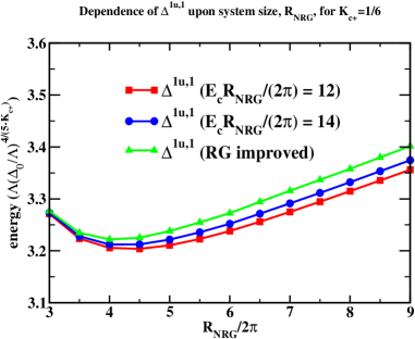
Figure 4: The value of $\Delta^{1u,1}$ for $K_{c+}=1/5$ as function of the system size, $R_{NRG}$, and the cutoff energy, $E_{c}$.

But we first turn to the easier of the gaps to determine: $\Delta^{1u,1}$, $\Delta^{1u,2}$, and $\Delta^{dark}$. For specificity we focus on $\Delta^{1u,1}$. Presented in Fig. 4 is $\Delta^{1u,1}$ as a function of system size, $R_{NRG}$, for two different truncations of the total number of states (15000 and 75000). (These truncations are determined by truncating the system so that the energies of the unperturbed states satisfy $R_{NRG}E/2\pi<12$ and $R_{NRG}E/2\pi<14$). We see that $\Delta^{1u,1}$ possesses only a weak dependence on $R_{NRG}$. This, however still leaves the question of which value of $R_{NRG}$ to use for $\Delta^{1u,1}$. For small values of $R_{NRG}$, we expect the energies of the full theory to reduce to that of the theory’s UV fixed point, i.e. we expect the energies to behave as $1/R_{NRG}$. We can see this behaviour beginning already at $R_{NRG}=6\pi$. For large values of $R_{NRG}$ we expect instead a truncation error (coming from ignoring higher energy states) of the form $R_{NRG}^{3/2-K_{c+}/2}$. This error typically leads to an overestimate of the true value of the gap. The slow increase of $\Delta^{1u,1}$ that begins at $R_{NRG}=10\pi$ is evidence of this. Given these behaviors (deviations of $\Delta^{1u,1}$ from its true value), it then makes sense to choose $R_{NRG}$ where $\Delta^{1u,1}$ is at its minimum. This we do by choosing $R_{NRG}=9\pi$.

The one cautionary note we make is that at this value of $R_{NRG}$, $\Delta^{1u,1}$ may still see finite size corrections. Even though $R_{NRG}$ is sufficiently large so that theory is far enough away from its UV fixed point, $\Delta^{1u,1}$ can see corrections related to virtual processes by which the excitation emits a virtual particle which then “travels around the world” and is reabsorbed. Such processes are suppressed exponentially in $R_{NRG}$ leading to small corrections to $\Delta^{1u,1}$, i.e. $\delta\Delta^{1u,1}\sim e^{-\alpha R}$. The coefficient $\alpha$ is either equal to $\Delta/v_{char}$ where $\Delta$ is one of the other gaps in the theory and $v_{char}$ is its characteristic velocity (a so-called F-term klas_mel ) or it is related to the binding energy associated with thinking of $\Delta^{1u,1}$ as a bound state of two other excitations (a so-called $\mu$-term klas_mel ). However for $\Delta^{1u,1}$, $\alpha$ (whether arising from an F-term or a $\mu$-term) is sufficiently large so that the correction should be small (it is difficult to make an absolute statement about this as we cannot easily estimate the coefficient in front of the exponential which in principle could be large). Believing it to be small we make no attempt directly to correct our results for this error. However dealing with finite size errors is necessary in studying the gaps $\Delta^{2g,1}$ and $\Delta^{1u,3}$.

We do however do a renormalization group improvement (RGI) of our numerical data by taking into account the RG flow that is occurring at fixed $R_{NRG}$. We see that as we increase the cutoff energy, $E_{c}$, the value of $\Delta^{1u,1}$ flows to smaller values. This flow, at lowest order, is governed by the equation

$$E_{c}\frac{d\delta\Delta^{1u,1}}{dE_{c}}=-\beta\delta\Delta^{1u,1},$$

where $\beta$ here is a function of the anomalous dimension of $H_{gap}$ and $\delta\Delta^{1u,1}=\Delta^{1u,1}(E_{c})-\Delta^{1u,1}(E_{c}=\infty)$. Integrating this equation, we can express the value of the gap at finite truncation energy to the gap at infinite truncation energy:

$$\Delta^{1u,1}(E_{c}=\infty)=\Delta^{1u,1}(E_{c})+\gamma/E_{c}^{-\beta},$$

where $\gamma$ is some constant. We thus can use the data for two different values of $E_{c}$ to estimate $\gamma$ and so extract the value of $\Delta^{1u,1}$ without cutoff. The results of doing so are plotted in Fig. 4 as $\Delta^{1u,1}~{}({\rm RG~{}improved})$.

To arrive at the value of $\Delta^{1u,1}$ actually reported in Fig. 2 of the manuscript, we assume the RG improved value represents an upper bound to the value of $\Delta^{1u,1}$ while the value of $\Delta^{1u,1}$ at $E_{c}R/2\pi=14$ represents a lower bound. It is then the average of these two values that is reported with the error bar being 1/2 the difference.

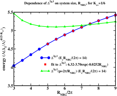
Figure 5: The value of $\Delta^{2g,1}$ for $K_{c+}=1/5$ as function of the system size, $R_{NRG}$, and the cutoff energy.

While $\Delta^{1u,1}$ does not suffer from significant finite size corrections, $\Delta^{2g,1}$ does. We show in Fig. 5 $\Delta^{2g,1}$ as a function of $R_{NRG}$. We see that unlike $\Delta^{1u,1}$, $\Delta^{2g,1}$ steadily increases as a function of $R_{NRG}$. We understand this to be a consequence of $\Delta^{2g,1}$ being a bound state of either two dark excitons, $\Delta^{dark}$, or two one-photon excitons, $\Delta^{1u,1}$, and that furthermore lies just below these two exciton thresholds, i.e $\Delta^{2g,1}$ is only slightly less than $2\Delta^{dark}$ or $2\Delta^{1u,1}$. In such circumstances strong finite size corrections are expected. These corrections take the form $\delta_{FS}\Delta^{2g,1}\sim\exp(-\alpha R_{NRG})$ where again $\alpha$ is related to the binding energy of the exciton. If $\Delta^{2g,1}$ is a bound state of the two dark excitons, $\alpha$ is given by

$$\alpha^{2}=(2\Delta^{dark}-\Delta^{2g,1})\frac{1}{2v_{0}^{2}},$$

where $v_{0}$ appears because the velocity of the dark excitons is very close to $v_{0}$ as they lie almost entirely in the spin/flavour sector of the theory. If instead $\Delta^{2g,1}$ is a bound state of two $\Delta^{1u,1}$, we have instead

$$\alpha^{2}=(2\Delta^{1u,1}-\Delta^{2g,1})\frac{1}{2v^{2}},$$

where $v$ here is approximately $v_{c+}$ but will not be exactly that as the exciton $\Delta^{1u,1}$ is influenced by both the charge and spin sectors of the theory. Thus if $\Delta^{2g,1}$ is close to either of the two exciton thresholds (or if $v$ is large which it likely is), $\alpha$ will be small and the finite size corrections, even though exponential, will decay only slowly as $R_{NRG}$ grows.

To estimate $\Delta^{2g,1}$, we assume the data to have the form $\Delta^{2g,1}(R_{NRG})=\Delta^{2g,1}(R=\infty)+\beta\exp(-\alpha R_{NRG})$. Fitting the data to this form allows us to estimate $\Delta^{2g,1}(R_{NRG}=\infty)$. We take this as an upper bound on the value of $\Delta^{2g,1}(R_{NRG}=\infty)$ as we expect that at larger $R_{NRG}$, $\Delta^{2g,1}$ is overestimated in the numerical data because of a finite cutoff, $E_{c}$. To find a lower bound, we examine $\Delta^{2g,1}$ as a function of momentum. Plotted in Fig. 5 is the numerical data for $\Delta^{2g,1}(p,R_{NRG})$ where the momentum $p$ is related to $R_{NRG}$ via $2\pi/R_{NRG}$. Where $\Delta^{2g,1}(p,R_{NRG})$ and $\Delta^{2g,1}(p=0,R_{NRG})$ meet then serves as a lower bound for $\Delta^{2g,1}$. (Incidentally the manner of this crossing indicates that the dispersion of $\Delta^{2g,1}$ at small momenta is hole-like, i.e. $\Delta^{2g,1}(p)\sim\Delta^{2g,1}-p^{2}/2m_{eff}$.) The value for $\Delta^{2g,1}$ that we plot in Fig. 5 of the manuscript is an average of these upper and lower bounds, while we take as an uncertainty 1/2 the difference of the two.

References

- (1) J. A. Misewich, R. Martel, Ph. Avouris, J. C. Tsang, S. Heinze, and J. Tersoff, Science 300, 783 (2003).
- (2) M. J. O’Connell et al., Science 297, 593 (2002).
- (3) J.-C. Charlier, X. Blase, and S. Roche, Rev. Mod. Phys. 79, 677 (2007).
- (4) F. Wang, G. Dukovic, L. Brus, T. F. Heinz, Science 308, 838 (2005).
- (5) O. N. Torrens, M. Zheng, and J. M. Kikkawa, Phys. Rev. Lett. 101, 157401 (2008).
- (6) H. Lin et al., Nature Materials 9, 235 (2010).
- (7) T. Ogawa, T. Takaghara, Phys. Rev. B 44, 8138 (1991).
- (8) H. Ajiki and T. Ando, J. Phys. Soc. Jph. 62, 1255 (1993); ibid. 65, 505 (1996); C. L. Kane and E. J. Mele, Phys. Rev. Lett. 78, 1932 (1997).
- (9) L. S. Levitov and A. M. Tsvelik, Phys. Rev. Lett. 90, 016401 (2003).
- (10) M. Rohlfing and S. G. Louie, Phys. Rev. B 62, 4927 (2000).
- (11) V. Perebeinos, J. Tersoff, and P. Avouris, Phys. Rev. Lett. 92, 257402 (2004).
- (12) C. L. Kane and E. J. Mele, Phys. Rev. Lett. 93, 197402 (2004).
- (13) V. Perebeinos, J. Tersoff, and P. Avouris, Nano Lett. 5, 2495 (2005).
- (14) J. Maultzsch, R. Pomraenke, S. Reich, E. Chang, D. Prezzi, A. Ruini, E. Molinari, M. S. Strano, C. Thomsen, and C. Lienau, Phys. Rev. B 72, 241402 (2005); D. Kammerlander, D. Prezzi, G. Goldoni, E. Molinari, U. Hohenester, Phys. Rev. Lett. 99, 126806 (2007).
- (15) J. Deslippe, M. Dipoppa, D. Prendergast, M. V. O. Moutinho, R. B. Capaz, S. G. Louie, Nano Lett. 9, 1330 (2009).
- (16) W. DeGottardi, T.-C. Wei, S. Vishveshwara, Phys. Rev. B 79, 205421 (2009).
- (17) R. Egger and A. O. Gogolin, Eur. Phys. J. B 3, 281 (1998).
- (18) C. Kane, L. Balents, M. P. A. Fisher, Phys. Rev. Lett. 79, 5086 (1997).
- (19) V. P. Yurov and Al. B. Zamolodchikov, Int. J. Mod. Phys. A 6, 4557 (1991).
- (20) R. M. Konik and Y. Adamov, Phys. Rev. Lett. 98, 147205 (2007).
- (21) R. M. Konik, supplementary material (at end of document).
- (22) S. Lukyanov and A. Zamolodchikov, Nucl. Phys. B. 493, 571 (1997).
- (23) Al. Zamolodchikov, J. Mod. Phys. A 10, 1125 (1995).
- (24) M. Lassig, G. Mussardo, and J. L. Cardy, Nucl. Phys. B 348, 591 (1991).
- (25) T. R. Klassen and E. Melzer, Nucl. Phys. B 362, 329 (1991).
- (26) G. Feverati, F. Ravanini, and G. Takacs, Phys. Lett. B 430, 264 (1998).
- (27) D. Fioravanti, G. Mussardo, and P. Simon, Phys. Rev. E 63, 016103 (2000).
- (28) Z. Bajnok, C. Dunning, L. Palla, G. Takacs, F. Wagner, Nucl. Phys. B 679, 521 (2004).
- (29) G. Takacs, F. Wagner, Nucl. Phys. B 741, 353 (2006).
- (30) L. Lepori, G. Mussardo, and G. Toth, J. Stat. Mech. (2008) P09004.
- (31) P. Di Francesco, P. Mathieu, and D. Seńećhal, Conformal Field Theory, Springer-Verlag, New York (1997).