Quantum anti-Zeno effect without wave function reduction

Abstract

We study the measurement-induced enhancement of the spontaneous decay (called quantum anti-Zeno effect) for a two-level subsystem, where measurements are treated as couplings between the excited state and an auxiliary state rather than the von Neumann’s wave function reduction. The photon radiated in a fast decay of the atom, from the auxiliary state to the excited state, triggers a quasi-measurement, as opposed to a projection measurement. Our use of the term “quasi-measurement” refers to a “coupling-based measurement”. Such frequent quasi-measurements result in an exponential decay of the survival probability of atomic initial state with a photon emission following each quasi-measurement. Our calculations show that the effective decay rate is of the same form as the one based on projection measurements. What is more important, the survival probability of the atomic initial state which is obtained by tracing over all the photon states is equivalent to the survival probability of the atomic initial state with a photon emission following each quasi-measurement to the order under consideration. That is because the contributions from those states with photon number less than the number of quasi-measurements originate from higher-order processes.

I Introduction

In the quantum Zeno effect (QZE) (see, e.g., Namiki97 ; Koshinoa05 ; Degasperis74 ; Teuscher04 ; Khalhin68 ; Misra77 ) frequent measurements inhibit atomic transitions for a closed system. In the quantum anti-Zeno effect (QAZE), atomic decays can be accelerated by frequent measurements, when the observed atom also interacts with a heat bath with some spectral distribution Lane83 ; Kofman00 ; Facchi01 ; Zheng08 ; Ai10 ; Ai10-2 ; Wang08 ; Zhou09 ; Cao10 . This QAZE has been extensively studied for various cases, such as the QAZE without the rotating-wave approximation Zheng08 ; Ai10 ; Cao10 ; Kofman04 and in an artificial bath Ai10-2 . The conventional explorations for the QAZE as well as the QZE need to invoke the von Neumann’s wave function collapse Neumann55 for quantum measurements, namely the projection measurement postulate. Thus, the QAZE seems to depend on a particular quantum mechanical interpretation specified by this collapse postulate.

However, even though the collapse postulate has been extensively used in the past, some researchers do not believe it is necessary for quantum mechanics. There exist other interpretations, such as the ensemble interpretation Ballentine70 . In this sense, it is necessary to develop a quantum-mechanical-interpretation-independent approach to the QAZE.

To this end, we draw lessons from the dynamic explanations for the QZE Petrosky ; Ballentine91 ; Block91 ; Frerichs91 . After the QZE was proposed by Misra and Sudarshan Misra77 , it was recognized Peres80 that the QZE could be mimicked by strong couplings to an external agent, which carried out a coupling-based detection. Then, an experiment Itano90 observing the QZE was explained Ballentine91 in such a dynamic fashion. Therein, all the phenomena were only described by the unitary evolution governed by the Schrödinger equation for the whole system. Later on, to further develop this dynamic interpretation of the QZE, Pascazio et al. Pascazio94 and Sun et al. Sun94 ; Sun95 explicitly used the decoherence model of quantum measurement, where the couplings to the apparatus only decohered the phases of the system rather than changed the system’s energy. This measurement model is essentially a non-demolition measurement Braginsky92 ; Ashhab09 .

Following these dynamic approaches for the QZE, we now develop a quantum dynamic theory for the QAZE without reference to projection measurements or the collapse postulate. To illustrate our main idea, we use an example, a two-level subsystem coupled to an auxiliary state to form a cascade configuration. Due to the couplings to the reservoir, the excited state spontaneously decays to the ground state. After a short interval, the remaining population of the excited state is coherently pumped into the auxiliary state by a strong laser. Then, it returns to the excited state by a fast spontaneous decay and a photon is emitted simultaneously. At this stage, a quasi-measurement is realized. Here, the term quasi-measurement refers to a coupling-based measurement in contrast to the usual projection measurement. The correlation of the atomic initial state and the orthogonal states with two orthogonal states of the environment is produced in such a process. We call it quasi-measurement since it can be viewed as the first (unitary) stage of the measurement process. Similar to the conventional approach, based on the collapse postulate, the effective decay rate of the survival probability with one photon emitted following each pulse in the presence of such quasi-measurements is given by the overlap integral of the measurement-induced level-broadening function and the interacting spectral distribution. As different photon states may not be distinguished in a realistic experiment, the survival probability of the atomic initial state after $n$ repetitive quasi-measurements, which can be obtained by tracing over all the photon states, can be taken into consideration. Since the contributions from photon states other than $n$ are due to higher-order processes, they lead to a small correction to the final result and can be omitted under the weak-coupling approximation in the short-time regime. Thus, the result for the projection measurements is recovered with the quasi-measurements.

The paper is organized as follows. In the next section, we describe the physical setup to realize the dynamic QAZE. In Sec. III, the effective decay rate of the survival probability with a photon emission following each pulse is obtained for repetitive quasi-measurements with a strong-intensity laser. The same result is also attained for the survival probability of the atomic initial state. Finally, we summarize the main results of the paper in Sec. IV. In order to make the paper self-consistent for reading, we present the detailed calculation for the free evolution under the short-time approximation in Appendix A.

II Model Setup

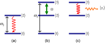
Figure 1: (Color online) Energy level diagram for the three processes considered here: (a) the spontaneous decay from the excited state $\left|2\right\rangle$ to the ground state $\left|1\right\rangle$, (b) a coherent transition with Rabi frequency $\Omega$ between $\left|2\right\rangle$ and the auxiliary state $\left|3\right\rangle$ by laser pumping, and (c) a fast spontaneous decay from $\left|3\right\rangle$ to $\left|2\right\rangle$ with a photon emitted in $\left|\gamma_{1}\right\rangle$. Here, the eigenenergies for the excited state and the auxiliary state are $\omega_{2}$ and $\omega_{3}$, respectively.

We consider the QAZE for a three-level atom with the cascade configuration depicted in Fig. 1(b,c). We mainly focus on the QAZE concerning a subsystem with the ground state $\left|1\right\rangle$ and the excited state $\left|2\right\rangle$. Since these two levels are coupled to a reservoir, there would be natural spontaneous decay from $\left|2\right\rangle$ to $\left|1\right\rangle$ if the subsystem were not coupled to other dynamic agents. In this process with duration $\tau$, the total system is governed by the Hamiltonian

$$H=\sum\limits_{k}\omega_{k}a_{k}^{{\dagger}}a_{k}+\omega_{2}\left|2\right\rangle\left\langle 2\right|+\sum\limits_{k}g_{k}(a_{k}^{{\dagger}}\left|1\right\rangle\left\langle 2\right|+\mathrm{H.c.})\text{,}$$ (1)

where $a_{k}$ ($a_{k}^{{\dagger}}$) is the annihilation (creation) operator for the reservoir’s $k$th mode with frequency $\omega_{k}$, $\omega_{2}$ the eigenenergy for the excited state $\left|2\right\rangle$, and $g_{k}$ the coupling constant between the $k$th mode and the transition between $\left|1\right\rangle$ and $\left|2\right\rangle$, which is assumed to be real for simplicity. We assume $\omega_{1}=0$. Notice that we have applied the rotating-wave approximation Scully97 to the above Hamiltonian (1).

In order to perform a quasi-measurement, we avoid the collapse-postulate, as also done, e.g., in Refs. Peres80 ; Petrosky ; Ballentine91 , where the quasi-measurement involved coherently coupling the measured state to an external agent, e.g., an additional energy level $\left|3\right\rangle$. In this sense, a quasi-measurement is the first (unitary) stage of the measurement process, providing an entanglement between the system and the apparatus. A quantum measurement in this approach is implemented by an alternative coupling lasting for $t_{p}$ between $\left|2\right\rangle$ and $\left|3\right\rangle$ with eigenenergy $\omega_{3}$, which is described by

$$H^{\prime} = \sum\limits_{k}\omega_{k}a_{k}^{{\dagger}}a_{k}+\omega_{2}\left|2\right\rangle\left\langle 2\right|+\omega_{3}\left|3\right\rangle\left\langle 3\right|$$ (2)

$$+\Omega\cos\Delta t(\left|2\right\rangle\left\langle 3\right|+\left|3\right\rangle\left\langle 2\right|)\text{,}$$

where $\Omega$ is the Rabi frequency between $\left|2\right\rangle$ and $\left|3\right\rangle$. Hereafter, we focus on the resonance case, i.e.,

$$\omega=\Delta\equiv\omega_{3}-\omega_{2}\text{.}$$ (3)

When the resonant coupling laser is applied between $\left|2\right\rangle$ and $\left|3\right\rangle$, we can disregard the spontaneous decay between the auxiliary state $\left|3\right\rangle$ and the excited state $\left|2\right\rangle$ for a very strong laser, i.e., $\Omega\gg\Gamma$ with $\Gamma$ being the decay rate from $\left|3\right\rangle$ to $\left|2\right\rangle$. Then, when the coupling laser is turned off, the population of the state $\left|3\right\rangle$ will quickly return to $\left|2\right\rangle$, with a photon $\gamma$ produced by the spontaneous decay, i.e.,

$$\left|3,v\right\rangle\rightarrow\left|2,\gamma_{1}\right\rangle\text{,}$$ (4)

where $\left|3,v\right\rangle=\left|3\right\rangle\left|v\right\rangle$ is the product state of the atomic auxiliary state $\left|3\right\rangle$ and the vacuum $\left|v\right\rangle$ for the reservoir, $\left|\gamma_{n}\right\rangle$ denotes the state with $n$ photons in the $\gamma$ mode. At this stage, the quasi-measurement is completed. Then, the subsystem alternatively evolves freely and is “measured” through laser pumping. The time sequence for the entire course is schematically shown in Fig. 2.

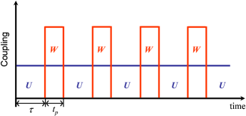
Figure 2: (Color online) The pulse sequence for demonstrating the QAZE by a quasi-measurement (i.e., avoiding projection measurements). Here, $U$ stands for the spontaneous decay from $\left|2\right\rangle$ to $\left|1\right\rangle$. Also, $W$ is a quasi-measurement which is alternatively present and absent for a duration $t_{p}$ and $\tau$, respectively.

Here, we assume the duration $1/\Gamma$ for the fast spontaneous decay from the auxiliary state $\left|3\right\rangle$ to the excited state $\left|2\right\rangle$ to be much smaller than the one for the spontaneous decay from $\left|2\right\rangle$ to $\left|1\right\rangle$, i.e., $1/\Gamma\ll\tau$. In this case, we can omit the dynamic evolution between $\left|2\right\rangle$ and $\left|1\right\rangle$ induced by the finite couplings to the reservoir when the fast spontaneous decay from the auxiliary state $\left|3\right\rangle$ to the excited state $\left|2\right\rangle$ occurs.

III Dynamical approach to the Anti-Zeno effect

In the previous section, we described a dynamical approach to study the QAZE. We emphasize that in our approach there is no wave-function-reduction postulate involved, and the unitary evolution of both the two-level subsystem and the measuring apparatus is depicted by means of the Schrödinger equation. Let us first describe the two basic processes $U$ and $W$ schematically illustrated in Fig. 2.

III.1 Spontaneous decay or $U$-process from $t=0$ to $\tau$

For the spontaneous decay between the excited state and the ground state, governed by the Hamiltonian (1), we assume the wave function of the total system to be a superposition of two kinds of single-excitation states, i.e.,

$$\left|\Psi(t)\right\rangle=\alpha(t)\left|2,v\right\rangle+\sum\limits_{k}\beta_{k}(t)\left|1,k\right\rangle\text{,}$$ (5)

where $\left|2,v\right\rangle=\left|2\right\rangle\left|v\right\rangle$ is the product state of the atomic excited state $\left|2\right\rangle$ and the vacuum $\left|v\right\rangle$ for the reservoir, $\left|1,k\right\rangle=\left|1\right\rangle\left|k\right\rangle$ the product state of the atomic ground state $\left|1\right\rangle$ and the single-excitation state $\left|k\right\rangle$ in the $k$th-mode of the reservoir. It follows from the Schrödinger equation $i\partial_{t}\left|\Psi(t)\right\rangle=H\left|\Psi(t)\right\rangle$ that the coefficients $\alpha(t)$ and $\beta_{k}(t)$ in Eq. (5) satisfy

$$i\dot{\alpha} = \omega_{2}\,\alpha+\sum\limits_{k}g_{k}\,\beta_{k}\text{,}$$ (6a)

$$i\dot{\beta}_{k} = \omega_{k}\,\beta_{k}+g_{k}\,\alpha\text{.}$$ (6b)

Under the short-time approximation, the solutions to the above equations become Kofman96

$$\alpha(t) = \alpha(0)\left[1+\sum\limits_{k}g_{k}^{2}\frac{h_{t}(\omega_{2}-\omega_{k})-it}{\omega_{2}-\omega_{k}}\right]e^{-i\omega_{2}t}$$ (7a)

$$-\sum\limits_{k}g_{k}\beta_{k}(0)h_{t}(\omega_{2}-\omega_{k})e^{-i\omega_{2}t}\text{,}$$

$$\beta_{k}(t) = \beta_{k}(0)e^{-i\omega_{k}t}+\alpha(0)g_{k}h_{t}(\omega_{2}-\omega_{k})e^{-i\omega_{2}t}\text{,}$$ (7b)

where

$$h_{t}(\omega)=\frac{1}{\omega}\left(e^{i\omega t}-1\right)\text{.}$$ (8)

The detailed calculations are presented in Appendix A.

III.2 Quasi-measurement or $W$-process from $t=\tau$ to $\tau+t_{p}$

In the quasi-measurement process, a strong laser field is applied to induce the transition between the excited state $\left|2\right\rangle$ and the auxiliary state $\left|3\right\rangle$ [see Fig. 1(b)]. With a unitary transformation

$$W=\exp(-i\Delta t\left|2\right\rangle\left\langle 2\right|)\text{,}$$ (9)

the transformed wave function $\left|\Psi^{\prime}(t)\right\rangle\equiv W\left|\Psi(t)\right\rangle$ is governed by the effective Hamiltonian $H_{\mathrm{eff}}\equiv WH^{\prime}W^{{\dagger}}-iW\partial_{t}W^{{\dagger}}$, which reads

$$H_{\mathrm{eff}}\simeq\sum\limits_{k}\omega_{k}a_{k}^{{\dagger}}a_{k}+\omega_{3}\left|2\right\rangle\left\langle 2\right|+\omega_{3}\left|3\right\rangle\left\langle 3\right|+\frac{\Omega}{2}(\left|2\right\rangle\left\langle 3\right|+\mathrm{H.c.})\text{,}$$ (10)

where we have dropped the fast-oscillating terms including the factors $\exp(\pm i2\Delta t)$.

Now we assume the transformed wave function to be

$$\left|\Psi^{\prime}(t)\right\rangle=A\left|2,v\right\rangle+\sum\limits_{k}B_{k}\left|1,k\right\rangle+C\left|3,v\right\rangle\text{.}$$ (11)

Then the original wave function $\left|\Psi(t)\right\rangle=W^{-1}\left|\Psi^{\prime}(t)\right\rangle$ can be written as

$$\left|\Psi(t)\right\rangle=Ae^{i\Delta t}\left|2,v\right\rangle+\sum\limits_{k}B_{k}\left|1,k\right\rangle+C\left|3,v\right\rangle\text{.}$$ (12)

According to the Schrödinger equation for the transformed wave function $i\partial_{t}\left|\Psi^{\prime}(t)\right\rangle=H_{\mathrm{eff}}\left|\Psi^{\prime}(t)\right\rangle$, we obtain the following system of differential equations

$$i\dot{A} = \omega_{2}A+\frac{\Omega}{2}Ce^{-i\Delta t}\text{,}$$ (13a)

$$i\dot{B}_{k} = \omega_{k}B_{k}\text{,}$$ (13b)

$$i\dot{C} = \omega_{3}C+\frac{\Omega}{2}Ae^{i\Delta t}\text{.}$$ (13c)

The solutions are given by

$$A(t) = \left[A(0)\cos\frac{\Omega}{2}t-iC(0)\sin\frac{\Omega}{2}t\right]e^{-i\omega_{2}t}\text{,}$$ (14a)

$$B_{k}(t) = B_{k}(0)e^{-i\omega_{k}t}\text{,}$$ (14b)

$$C(t) = \left[C(0)\cos\frac{\Omega}{2}t-iA(0)\sin\frac{\Omega}{2}t\right]e^{-i\omega_{3}t}\text{.}$$ (14c)

Applying a $\pi$-pulse, i.e., a laser with duration

$$t_{p}=\frac{\pi}{\Omega}\text{,}$$ (15)

drives the system to evolve into the state

$$\left|\Psi(t_{p})\right\rangle=\sum\limits_{k}B_{k}(t_{p})\left|1,k\right\rangle+C(t_{p})\left|3,v\right\rangle\text{,}$$ (16)

where the coefficients

$$B_{k}(t_{p}) = B_{k}(0)e^{-i\omega_{k}t_{p}}\text{,}$$ (17a)

$$C(t_{p}) = -iA(0)e^{-i\omega_{3}t_{p}}$$ (17b)

can be obtained from Eq. (14). Here, we have assumed there is no initial population in the auxiliary state, namely $$C(0)=0 A(t_{p})=0 \left|3,v\right\rangle \left|2,\gamma_{1}\right\rangle$$, and thus . Afterwards, by means of a fast spontaneous decay, the state decays into [see Fig. 1(c)]. Therefore, a quasi-measurement is finished.

III.3 Repetition of the decay and quasi-measurement processes

Here, we will explicitly describe the complete process including the free evolution by $U$ and the quasi-measurement by $W$. The total system is initially prepared in the excited state with the reservoir in the vacuum: $\left|\Psi(0)\right\rangle=\left|2,v\right\rangle$. Then, after a free evolution with period $\tau$, the state evolves into

$$\left|\Psi(\tau)\right\rangle=\alpha^{(1,0)}(\tau)\left|2,v\right\rangle+\sum\limits_{k}\beta_{k}^{(1,0)}(\tau)\left|1,k\right\rangle\text{,}$$ (18)

where

$$\alpha^{(1,0)}(\tau)\!\!\!\! = \!\!\!\!\left[1+\sum\limits_{k}g_{k}^{2}\frac{h_{\tau}(\omega_{2}-\omega_{k})-i\tau}{\omega_{2}-\omega_{k}}\right]e^{-i\omega_{2}\tau}\text{,}$$ (19a)

$$\beta_{k}^{(1,0)}(\tau)\!\!\!\! = \!\!\!\!g_{k}h_{\tau}(\omega_{2}-\omega_{k})e^{-i\omega_{2}\tau}\text{.}$$ (19b)

Applying a strong laser forces the system to evolve into

$$\left|\Psi(\tau+t_{p})\right\rangle=C(t_{p})\left|3,v\right\rangle+\sum\limits_{k}\beta_{k}^{(1,0)}(\tau)\left|1,k\right\rangle$$ (20)

with

$$C(t_{p})=-i\alpha^{(1,0)}(\tau)e^{-i\omega_{3}t_{p}}\text{.}$$ (21)

Later, through a fast spontaneous decay, the total system becomes

$$\left|\Psi(\tau+t_{p}+t_{d})\right\rangle=C(t_{p})\left|2,\gamma_{1}\right\rangle+\sum\limits_{k}\beta_{k}^{(1,0)}(\tau)\left|1,k\right\rangle\text{.}$$

At this stage, the first cycle is accomplished. The survival probability amplitude of the state $\left|2\right\rangle$ after one quasi-measurement is $C(t_{p})$. Hereafter, for the sake of simplicity, we will label $\left|\Psi\left(n\tau+(n-1)t_{p}+(n-1)t_{d}\right)\right\rangle$, $\left|\Psi\left(n\tau+nt_{p}+(n-1)t_{d}\right)\right\rangle$, and $\left|\Psi\left(n\left(\tau+t_{p}+t_{d}\right)\right)\right\rangle$ as $\left|\Psi_{n}(1)\right\rangle$, $\left|\Psi_{n}(2)\right\rangle$, and $\left|\Psi_{n}(3)\right\rangle$, respectively. In other words, $\left|\Psi_{n}(j)\right\rangle$ denotes the state after $j$th procedure in the $n$th cycle for $n=1,2,\cdots$ and $j=1,2,3$.

For the second cycle, after the free evolution, the total system is in the state

$$\left|\Psi_{2}(1)\right\rangle = C(t_{p})\left[\alpha^{(1,0)}(\tau)\left|2\right\rangle+\sum\limits_{k}\beta_{k}^{(1,0)}(\tau)\left|1,k\right\rangle\right]\left|\gamma_{1}\right\rangle$$ (22)

$$+\alpha^{(2,1)}(\tau)\left|2,v\right\rangle+\sum\limits_{k}\beta_{k}^{(2,1)}(\tau)\left|1,k\right\rangle\text{,}$$

where the coefficients

$$\alpha^{(2,1)}(\tau) = \sum\limits_{k}\left[\beta_{k}^{(1,0)}(\tau)\right]^{2}\text{,}$$ (23a)

$$\beta_{k}^{(2,1)}(\tau) = \beta_{k}^{(1,0)}(\tau)e^{-i\omega_{k}\tau}$$ (23b)

are determined by Eq. (7) with initial conditions

$$\alpha^{(2,1)}(0)=0\text{,}\;\;\;\beta_{k}^{(2,1)}(0)=\beta_{k}^{(1,0)}(\tau)\text{.}$$

After another $\pi$-pulse,

$$\left|\Psi_{2}(2)\right\rangle = C(t_{p})\left[\sum\limits_{k}\beta_{k}^{(1,0)}(\tau)\left|1,k\right\rangle+C(t_{p})\left|3\right\rangle\right]\left|\gamma_{1}\right\rangle$$ (24)

$$+\sum\limits_{k}\beta_{k}^{(2,1)}(\tau)\left|1,k\right\rangle+C^{(2,1)}(t_{p})\left|3,v\right\rangle\text{,}$$

where

$$C^{(2,1)}(t_{p})=-i\sum\limits_{k}\left[\beta_{k}^{(1,0)}(\tau)\right]^{2}e^{-i\omega_{3}t_{p}}\text{.}$$ (25)

Afterwards, by means of a fast spontaneous decay it becomes

$$\left|\Psi_{2}(3)\right\rangle\!\!\!\! = \!\!\!\!C(t_{p})\sum\limits_{k}\beta_{k}^{(1,0)}(\tau)\left|1,k\right\rangle\left|\gamma_{1}\right\rangle+\sum\limits_{k}\beta_{k}^{(2,1)}(\tau)\left|1,k\right\rangle$$ (26)

$$\!\!\!\!+C^{2}(t_{p})\left|2,\gamma_{2}\right\rangle+C^{(2,1)}(t_{p})\left|2,\gamma_{1}\right\rangle\text{.}$$

Thus, the survival probability of the state $\left|2\right\rangle$ with photon emissions following both pulses is $\left|C^{2}(t_{p})\right|^{2}$. Here, we point out that this is different from the survival probability of the atomic initial state, which has an additional contribution from $\left|2,\gamma_{1}\right\rangle$. In this dynamic approach for the QAZE, once a photon in the $\gamma$ mode is emitted right after a pulse, a quasi-measurement is finished. This means that the system is in the initial state before the quasi-measurement and still remains in its initial state after the quasi-measurement. For the case with two quasi-measurements, $C^{(2,1)}(t_{p})$ corresponds to such a probability amplitude which decays to the ground state before the first quasi-measurement and returns to the excited state before the second quasi-measurement.

III.4 Survival probability describing the anti-Zeno effect

By means of mathematical induction, we can prove the wave function of the total system after $n$ quasi-measurements to be of the following form

$$\left|\Psi_{n}(3)\right\rangle = C^{n}(t_{p})\left|2,\gamma_{n}\right\rangle+\sum\limits_{j=1}^{n-1}C^{(n,j)}(t_{p})\left|2,\gamma_{j}\right\rangle$$ (27)

$$+C^{n-1}(t_{p})\sum\limits_{k}\beta_{k}^{(1,0)}(\tau)\left|1,k\right\rangle\left|\gamma_{n-1}\right\rangle$$

$$+\sum\limits_{j=1}^{n-1}\sum\limits_{k}\beta_{k}^{(n,j)}(\tau)\left|1,k\right\rangle\left|\gamma_{j-1}\right\rangle\text{,}$$

where

$$C^{(n,j)}(t_{p})\sim\sum\limits_{k}\left[\beta_{k}^{(1,0)}(\tau)\right]^{2}$$ (28)

for $j<n$. Judging from the analysis made in the previous section, we may safely arrive at the conclusion that the survival probability amplitude of the state $\left|2\right\rangle$ with photon emissions following $n$ pulses is $C^{n}(t_{p})$. It is straightforward to calculate the survival probability as

$$P_{2}(t=n\tau)=\left|C(t_{p})\right|^{2n}\text{.}$$ (29)

As a result, we observe an exponential decay of the survival probability of the atomic initial state with photon emission following each pulse, i.e., $P_{2}(t)=\exp(-Rt)$. Here, the effective decay rate is

$$R(\tau)=2\pi\int_{-\infty}^{\infty}F(\omega,\tau)G(\omega)d\omega\text{,}$$ (30)

where the interacting spectral distribution is

$$G(\omega)=\sum\limits_{k}g_{k}^{2}\delta(\omega-\omega_{k})=g_{k}^{2}\rho(\omega_{k})|_{\omega_{k}=\omega}\text{,}$$ (31)

with $\rho(\omega)$ being the density of state for $\omega$, the measurement-induced level-broadening function

$$F(\omega,\tau)=\frac{\tau}{2\pi}\text{sinc}^{2}\left[\frac{1}{2}(\omega_{2}-\omega)\tau\right]\text{.}$$ (32)

Besides, we resort to the numerical simulation for the $2p$-$1s$ transition of hydrogen atom with the interacting spectral distribution Moses73

$$G(\omega)=\frac{\eta\omega}{[1+(\frac{\omega}{\omega_{c}})^{2}]^{4}}\text{,}$$ (33)

where $\eta=6.435\times 10^{-9}$, $\omega_{c}=8.491\times 10^{18}$ rad/s. As shown in Fig. 3, the transition from the QAZE to the QZE, which is the same as the one predicted by the projection measurement Kofman00 , is observed by varying the quasi-measurement interval $\tau$. Here, the short interval for the QZE is roughly of the order of $1/\omega_{c}$ Facchi98 .

On the other hand, in a realistic experiment, on condition that the state $\left|2,\gamma_{n}\right\rangle$ can not be distinguished from those states $\left|2,\gamma_{j}\right\rangle$ with $j$ less than $n$, the survival probability of the initial state $\left|2\right\rangle$ is obtained by tracing over all the possible photon states. In this case, the survival probability of the atomic initial state reads

$$P_{2}^{T}(t)=\left|C^{n}(t_{p})\right|^{2}+\sum\limits_{j=1}^{n-1}\left|C^{(n,j)}(t_{p})\right|^{2}\text{.}$$ (34)

As seen in Eq. (28), the contribution from the second term on the right hand side of Eq. (34) is of higher-order correction to the final result in the weak-coupling case. Thus, the survival probability of the atomic initial state including the contributions from all the photon states also displays an exponential decay with the effective decay rate being of the same form in Eq. (30). This is a physical result and its reason will be presented as follows. After the $n$th cycle, $C^{(n,j)}(t_{p})$ is the probability amplitude for $\left|2,\gamma_{j}\right\rangle$, which stands for $j$ photons emitted in $n$ quasi-measurements. Take $C^{(n,n-1)}(t_{p})$ for an example. It corresponds to such a probability amplitude which decays into the ground state before one quasi-measurement and returns to the initial state before the next quasi-measurement. For the other $n-2$ quasi-measurements, it always stays in the initial state before the quasi-measurements. Since the transition probability amplitude between $\left|2\right\rangle$ and $\left|1,k\right\rangle$ is $g_{k}$, the probability amplitude for the atomic excited state to first decay into the ground state and then return is proportional to $g_{k}^{2}$. As a result, the corresponding probability $\left|C^{(n,n-1)}(t_{p})\right|^{2}$ is of the order of $g_{k}^{4}$. Similar analyses can also be applied to $\left|C^{(n,j)}(t_{p})\right|^{2}$ when $j<n-1$. In a word, the second term on the right hand side of Eq. (34) can be neglected due to its characteristics of higher-order correction.

Since the above analysis is based on the weak-coupling approximation, a natural question comes into our minds. That is under what condition the second term on the right hand side of Eq. (34) can be disregarded. A straightforward calculation shows

$$\left|\sum\limits_{k}\left[\beta_{k}^{(1,0)}(\tau)\right]^{2}\right|^{2}\ll\text{Re}\sum\limits_{k}\frac{g_{k}^{2}h_{\tau}(\omega_{2}-\omega_{k})}{\omega_{2}-\omega_{k}}$$ (35)

with Re$(x)$ being the real part of $x$. Here, the term on the right hand side of Eq. (35) corresponds to the second order term in Eq. (29), while the term on the left hand side of Eq. (35) corresponds to the second term on the right hand side of Eq. (34). Mathematically speaking, the interacting spectrum $G(\omega)$ should be sufficiently broad and smooth. This is similar to the quantitative criterion obtained for the spontaneous decay to a continuum with photonic band gaps Kofman94 . In the case with strong couplings, the return of the excitation from the final state may be significant for sufficiently-long times as already shown in Refs. Milburn88 ; Kofman01 , where the free evolution was due to a classical field.

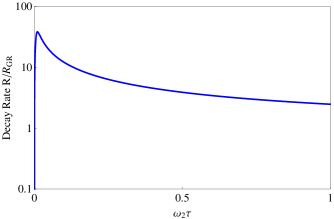
Figure 3: (Color online) The effective decay rate $R(\tau)$ versus quasi-measurement interval $\tau$ for the $2p$-$1s$ transition of the hydrogen atom with $\omega_{2}=1.55\times 10^{16}$ rad/s.

IV Conclusion

In this paper, we investigated the QAZE for a two-level subsystem embedded in a three-level atom. Instead of considering projection measurements, we studied quasi-measurements by pumping the population of the excited state to an auxiliary state. Since the pumped population returns to the excited state by a fast spontaneous decay, the complete process of the quasi-measurement is finished. Along with the fast spontaneous decay, there is a photon emitted in the corresponding mode.

We found that the effective decay rate of the survival probability still remains as the overlap integral of the measurement-induced level-broadening function and the interacting spectral distribution. Moreover, it is discovered that the survival probability of the atomic initial state is the same as the survival probability of the atomic initial state with photon emission following each pulse since the difference between them leads to a higher-order correction. This is because the contributions from the other photon states originate from higher-order processes. In conclusion, without projection measurements, we can observe the QAZE and the QZE by means of quasi-measurements.

Generally speaking, the QZE and QAZE stem from frequent decoherence events, which destroy the off-diagonal density matrix elements. When the diagonal elements in the density matrix remain unchanged after these processes, the above decoherence is actually dephasing between the initial and final states, e.g., between the first and second terms on the right hand side of Eq. (5). And the model in this paper is just of such kind. Other methods include measurements as in Refs. Pascazio94 ; Sun94 ; Sun95 ; Milburn88 ; Facchi05 , and even a classical random field Harel98 . Note that the above decoherence can take effect due to not only dephasing, but also a destruction of the final states Kwiat98 ; Kofman01 . On the other hand, the decoherence can be suppressed by a train of ultrafast off-resonant optical pulses Search00 .

Appendix A Time Evolution in Spontaneous Decay

In this Appendix, we present the detailed calculations for the free evolution. By defining the slowly-varying variables

$$\alpha^{\prime}(t) = \alpha e^{i\omega_{2}t}\text{,}$$ (36)

$$\beta_{k}^{\prime}(t) = \beta_{k}e^{i\omega_{k}t}\text{,}$$ (37)

we obtain a system of simplified equations from Eq. (6)

$$i\dot{\alpha}^{\prime} = \sum\limits_{k}g_{k}\beta_{k}^{\prime}e^{i(\omega_{2}-\omega_{k})t}\text{,}$$ (38)

$$i\dot{\beta}_{k}^{\prime} = g_{k}\alpha^{\prime}e^{-i(\omega_{2}-\omega_{k})t}\text{.}$$ (39)

We can integrate Eq. (39) to have a formal solution for $\beta_{k}^{\prime}(t)$, i.e.,

$$\beta_{k}^{\prime}(t) = \beta_{k}^{\prime}(0)-i\int\limits_{0}^{t}g_{k}\alpha^{\prime}(t^{\prime})e^{i(\omega_{k}-\omega_{2})t^{\prime}}dt^{\prime}$$ (40)

$$\simeq \beta_{k}^{\prime}(0)-i\alpha^{\prime}(0)\int\limits_{0}^{t}g_{k}e^{i(\omega_{k}-\omega_{2})t^{\prime}}dt^{\prime}$$

$$= \beta_{k}(0)-\alpha(0)g_{k}h_{t}(\omega_{k}-\omega_{2})\text{,}$$

where in the second line we have used the short-time approximation $\alpha^{\prime}(t^{\prime})\simeq\alpha^{\prime}(0)$ and $h_{t}(\omega)$ given by Eq. (8). By substituting Eq. (40) into Eq. (38) and making use of the short-time approximation, we have

$$\alpha^{\prime}(t)\!\!\! = \!\!\!\alpha^{\prime}(0)-i\sum\limits_{k}\int\limits_{0}^{t}g_{k}\beta_{k}^{\prime}(t^{\prime})e^{-i(\omega_{k}-\omega_{2})t^{\prime}}dt^{\prime}$$ (41)

$$\simeq \!\!\!\alpha(0)\left[1+\sum\limits_{k}g_{k}^{2}\frac{h_{t}(\omega_{2}-\omega_{k})-it}{\omega_{2}-\omega_{k}}\right]$$

$$\!\!\!-\sum\limits_{k}g_{k}\beta_{k}(0)h_{t}(\omega_{2}-\omega_{k})\text{.}$$

In order to obtain the explicit forms of $\alpha$ and $\beta_{k}$, we shall use the inverse transform of Eqs. (36) and (37),

$$\alpha(t) = \alpha(0)\left[1+\sum\limits_{k}g_{k}^{2}\frac{h_{t}(\omega_{2}-\omega_{k})-it}{\omega_{2}-\omega_{k}}\right]e^{-i\omega_{2}t}$$ (42)

$$-\sum\limits_{k}g_{k}\beta_{k}(0)h_{t}(\omega_{2}-\omega_{k})e^{-i\omega_{2}t}\text{,}$$

and $\beta_{k}(t)$ given by Eq. (7b).