Bayesian inference for exponential random graph models

Abstract

Exponential random graph models are extremely difficult models to handle from a statistical viewpoint, since their normalising constant, which depends on model parameters, is available only in very trivial cases. We show how inference can be carried out in a Bayesian framework using a MCMC algorithm, which circumvents the need to calculate the normalising constants. We use a population MCMC approach which accelerates convergence and improves mixing of the Markov chain. This approach improves performance with respect to the Monte Carlo maximum likelihood method of Geyer and Thompson (1992).

Bayesian inference for exponential random graph models

1 Introduction

Our motivation for this article is to propose Bayesian inference for estimating exponential random graph models (ERGMs) which are some of the most important models in many research areas such as social networks analysis, physics and biology. The implementation of estimation methods for these models is a key point which enables us to use parameter estimates as a basis for simulation and to reproduce features of real networks. Unfortunately, the intractability of the normalising constant and degeneracy are two strong barriers to parameter estimation for these models. The classical inferential methods such as the Monte Carlo maximum likelihood (MC-MLE) of Geyer and Thompson (1992) and pseudolikelihood estimation (MPLE) of Besag (1974) and Strauss and Ikeda (1990), are very widely used in partice, but are lacking in certain respects. In some instance it is difficult to obtain reasonable results or to understand the properties of the approximations, using these methods.

The Bayesian estimation approach for these models has not yet been deeply and fully explored. Despite this, Bayesian inference is very appropriate in this context since it allows uncertainty about model parameters given the data to be explored through a posterior distribution. Moreover the Bayesian approach allows a formal comparison procedure among different competing models using posterior probabilities. Therefore the methods presented in this work aim to contribute to the development of a Bayesian-based methodology area for these models.

Networks are relational data represented as graphs, consisting of nodes and edges. Many probability models have been proposed in order to summarise the general structure of graphs by utilising their local properties. Each of these models take different assumptions into account: the Bernoulli random graph model (Erdös and Rényi, 1959) in which edges are considered independent of each other; the $p_{1}$ model (Holland and Leinhardt, 1981) where dyads are assumed independent, and its random effects variant the $p_{2}$ model (van Duijn et al., 2004); and the Markov random graph model (Frank and Strauss, 1986) where each pair of edges is conditionally dependent given the rest of the graph. The family of exponential random graph models (Wasserman and Pattison (1996), see also Robins et al. (2007b) for a recent review) is a generalisation of the latter model and has been thought to be a flexible way to model the complex dependence structure of network graphs. Recent developments have led to the introduction of new specifications by Snijders et al. (2006) and the implementation of curved exponential random graph models by Hunter and Handcock (2006). New modelling alternatives such as the latent variable models have been proposed by Hoff et al. (2002) under the assumption that each node of the graph has a unknown position in a latent space and the probability of the edges are functions of those positions and node covariates. The latent position cluster model of Handcock et al. (2007b) represents a further extension of this approach that takes account of clustering. Stochastic blockmodel methods (Nowicki and Snijders, 2001) involve block model structures whereby nodes of the graph are partitioned into latent classes and their relationship depends on block membership. More recently, the mixed membership approach (Airoldi et al., 2008) has emerged as a flexible modelling tool for networks extending the assumption of a single block membership.

In this paper we are concerned with Bayesian inference for exponential random graph models. This leads to the problem of the double intractability of the posterior density as both the model and the posterior normalisation terms cannot be evaluated. This problem can be overcome by adapting the exchange algorithm of Murray et al. (2006) to the network graph framework. Typically the high posterior density region is thin and highly correlated. For this reason, we also propose to use a population-based MCMC approach so as to improve the mixing and local moves on the high posterior density region reducing the chain’s autocorrelation significantly. An R package called Bergm, which accompanies this paper, contains all the procedures used in this paper. It can be found at: http://cran.r-project.org/web/packages/Bergm/.

This article is structured as follows. A basic description of exponential random graph models together with a brief illustration of the issue of degeneracy is given in Section 2. Section 3 reviews two of the most important and used methods for likelihood inference. In Section 4 we introduce Bayesian inference via the exchange algorithm and its further improvement through a population-based MCMC procedure. In Section 5 we fit different models to three benchmark network datasets and outline some conclusions in Section 6.

2 Exponential random graph models

Typically networks consist of a set of actors and relationships between pairs of them, for example social interactions between individuals. The network topology structure is measured by a random adjacency matrix $Y$ of a graph on $n$ nodes (actors) and a set of edges (relationships) $\{Y_{ij}:i=1,\dots,n;j=1,\dots,n\}$ where $Y_{ij}=1$ if the pair $(i,j)$ is connected, and $Y_{ij}=0$ otherwise. Edges connecting a node to itself are not allowed so $Y_{ii}=0$. The graph $Y$ may be directed (digraph) or undirected depending on the nature of the relationships between the actors.
Let $\mathcal{Y}$ denote the set of all possible graphs on $n$ nodes and let $y$ a realisation of $Y$. Exponential random graph models (ERGMs) are a particular class of discrete linear exponential families which represent the probability distribution of $Y$ as

$$\pi(\hbox{\boldmath$y$}|\hbox{\boldmath$\theta$})=\frac{q_{\hbox{\boldmath$\theta$}}(\hbox{\boldmath$y$})}{z(\hbox{\boldmath$\theta$})}=\frac{\exp\{\hbox{\boldmath$\theta$}^{t}s(\hbox{\boldmath$y$})\}}{z(\hbox{\boldmath$\theta$})}$$ (1)

where $s(\hbox{\boldmath$y$})$ is a known vector of sufficient statistics (e.g. the number of edges, degree statistics, triangles, etc.) and $\hbox{\boldmath$\theta$}\in\Theta$ are model parameters. Since $\mathcal{Y}$ consists of $2^{\binom{n}{2}}$ possible undirected graphs, the normalising constant $z(\hbox{\boldmath$\theta$})=\sum_{\hbox{\boldmath$y$}\in\mathcal{Y}}\exp\{\hbox{\boldmath$\theta$}^{t}s(\hbox{\boldmath$y$})\}$ is extremely difficult to evaluate for all but trivially small graphs. For this reason, ERGMs are very difficult to handle in practice. In spite of this difficulty, ERGMs are very popular in the literature since they are conceived to capture the complex dependence structure of the graph and allow a reasonable interpretation of the observed data. The dependence hypothesis at the basis of these models is that edges self organize into small structures called configurations. There is a wide range of possible network configurations (Robins et al., 2007a) which give flexibility to adapt to different contexts. A positive parameter value for $\theta_{i}\in\hbox{\boldmath$\theta$}$ result in a tendency for the certain configuration corresponding to $s_{i}(\hbox{\boldmath$y$})$ to be observed in the data than would otherwise be expected by chance.

2.1 Degeneracy

Degeneracy is one of the most important aspects of random graph models: it refers to a probability model defined by a certain value of $\theta$ that places most of its mass on a small number of graph topologies, for example, empty graphs or complete graphs.

Consider the mean value parametrisation for the model (1) defined by $\mu(\hbox{\boldmath$\theta$})={\mathbb{E}}_{\hbox{\boldmath$\theta$}}[s(\hbox{\boldmath$y$})]$. Let $C$ be the convex hull of the set $\{s(\hbox{\boldmath$y$}):\hbox{\boldmath$y$}\in\mathcal{Y}\}$, $ri(C)$ its relative interior and $rbd(C)$ its relative boundary. It turns out that if the expected values $\mu(\hbox{\boldmath$\theta$})$ of the sufficient statistics $\mu(\hbox{\boldmath$\theta$})$ approach the boundary $rbd(C)$ of the hull, the model places most of the probability mass on a small set of graphs belonging to $deg(\mathcal{Y})=\{\hbox{\boldmath$y$}\in\mathcal{Y}:s(\hbox{\boldmath$y$})\in rbd(C)\}$. It is also known that the MLE exists if and only if $s(\hbox{\boldmath$y$})\in ri(C)$ and if it exists it is unique.

When the model is near-degenerate, MCMC inference methods may fail to find the maximum likelihood estimate (MLE) and returning an estimate of $\theta$ that is unlikely to generate networks closely resembling the observed graph. This is because the convergence of the algorithm may be greatly affected by degenerate parameters values which during the network simulation process may yield graphs which are full or empty.

A more detailed description of this issue can be found in Handcock (2003) and Rinaldo et al. (2009). The new specifications proposed by Snijders et al. (2006) can often mitigate degeneracy and provide reasonable fit to the data.

3 Classical inference

3.1 Maximum pseudolikelihood estimation

A standard approach to approximate the distribution of a Markov random field is to use a maximum pseudolikelihood (MPLE) approximation, first proposed in Besag (1974) and adapted for social network models in Strauss and Ikeda (1990). This approximation consists of a product of easily normalised full-conditional distributions

$$\pi(\hbox{\boldmath$y$}|\hbox{\boldmath$\theta$})\approx\pi_{pseudo}(\hbox{\boldmath$y$}|\hbox{\boldmath$\theta$}) =\prod_{i\neq j}\pi(y_{ij}|\hbox{\boldmath$y$}_{-ij},\hbox{\boldmath$\theta$})$$ (2)

$$=\prod_{i\neq j}\frac{\pi(y_{ij}=1|\hbox{\boldmath$y$}_{-ij},\hbox{\boldmath$\theta$})^{y_{ij}}}{\left[1-\pi(y_{ij}=0|\hbox{\boldmath$y$}_{-ij},\hbox{\boldmath$\theta$})\right]^{y_{ij}-1}}$$

where $\hbox{\boldmath$y$}_{-ij}$ denotes all the dyads of the graph excluding $y_{ij}$. The basic idea underlying this method is the assumption of weak dependence between the variables in the graph so that the likelihood can be well approximated by the pseudolikelihood function. This leads to fast estimation. Nevertheless this approach turns out to be generally inadequate since it only uses local information whereas the structure of the graph is affected by global interaction. In the context of the autologistic distribution in spatial statistics, Friel et al. (2009) showed that the pseudolikelihood estimator can lead to inefficient estimation.

3.2 Monte Carlo maximum likelihood estimation

There are many instances of statistical models with intractable normalising constants. This general problem was tackled in Geyer and Thompson (1992) who introduced the Monte Carlo maximum likelihood (MC-MLE) algorithm. In the context of ERGMs, a key identity is the following

$$\frac{z(\hbox{\boldmath$\theta$})}{z(\hbox{\boldmath$\theta$}_{0})}={\mathbb{E}}_{\hbox{\boldmath$y$}|\hbox{\boldmath$\theta$}_{0}}\left[\frac{q_{\hbox{\boldmath$\theta$}}(\hbox{\boldmath$y$})}{q_{\hbox{\boldmath$\theta$}_{0}}(\hbox{\boldmath$y$})}\right]=\sum_{\hbox{\boldmath$y$}}\frac{q_{\hbox{\boldmath$\theta$}}(\hbox{\boldmath$y$})}{q_{\hbox{\boldmath$\theta$}_{0}}(\hbox{\boldmath$y$})}\frac{q_{\hbox{\boldmath$\theta$}_{0}}(\hbox{\boldmath$y$})}{z(\hbox{\boldmath$\theta$}_{0})}$$ (3)

where $q_{\hbox{\boldmath$\theta$}}(\cdot)$ is the unnormalised likelihood of parameters $\theta$, $\hbox{\boldmath$\theta$}_{0}$ is fixed set of parameter values, and ${\mathbb{E}}_{\hbox{\boldmath$y$}|\hbox{\boldmath$\theta$}_{0}}$ denotes an expectation taken with respect to the distribution $\pi(\hbox{\boldmath$y$}|\hbox{\boldmath$\theta$}_{0})$. In practice this ratio of normalising constants is approximated using graphs $\hbox{\boldmath$y$}_{1},\dots,\hbox{\boldmath$y$}_{m}$ sampled via MCMC from $\pi(\hbox{\boldmath$y$}|\hbox{\boldmath$\theta$}_{0})$ and importance sampling. This yields the following approximated log likelihood ratio:

$$w_{\hbox{\boldmath$\theta$}_{0}}(\hbox{\boldmath$\theta$})=\ell(\hbox{\boldmath$\theta$})-\ell(\hbox{\boldmath$\theta$}_{0})\approx(\hbox{\boldmath$\theta$}-\hbox{\boldmath$\theta$}_{0})^{t}s(\hbox{\boldmath$y$})-\log\left[\frac{1}{m}\sum_{i=1}^{m}\exp\left\{(\hbox{\boldmath$\theta$}-\hbox{\boldmath$\theta$}_{0})^{t}s(\hbox{\boldmath$y$}_{i})\right\}\right]$$ (4)

where $\ell(\cdot)$ is the log-likelihood. $w_{\hbox{\boldmath$\theta$}_{0}}$ is a function of $\theta$, and its maximum value serves as a Monte Carlo estimate of the MLE.

A crucial aspect of this algorithm is the choice of $\hbox{\boldmath$\theta$}_{0}$. Ideally $\hbox{\boldmath$\theta$}_{0}$ should be very close to the maximum likelihood estimator of $\theta$. Viewed as a function of $\theta$, $w_{\hbox{\boldmath$\theta$}_{0}}(\hbox{\boldmath$\theta$})$ in (4) is very sensitive to the choice of $\hbox{\boldmath$\theta$}_{0}$. A poorly chosen value of $\hbox{\boldmath$\theta$}_{0}$ may lead to an objective function (4) that cannot even be maximised. We illustrate this point in Section 3.4.

In pratice, $\hbox{\boldmath$\theta$}_{0}$ is often chosen as the maximiser of (2), although this itself maybe a very biased estimator. Indeed, (4) may also be sensitive to numerical instability, since it effectively computes the ratio of a normalising constant, but it is well understood that the normalising constants can vary by orders of magnitude with $\theta$.

In fact, if the value of $\hbox{\boldmath$\theta$}_{0}$ lies in the “degenerate region” then graphs $\hbox{\boldmath$y$}_{i},\dots,\hbox{\boldmath$y$}_{m}$ simulated from $\pi(\hbox{\boldmath$y$}|\hbox{\boldmath$\theta$}_{0})$ will tend to belong to $deg(\mathcal{Y})$ and hence the estimate of the ratio of normalising constants $z(\hbox{\boldmath$\theta$})/z(\hbox{\boldmath$\theta$}_{0})$ will be very poor. Consequently $w_{\hbox{\boldmath$\theta$}_{0}}(\hbox{\boldmath$\theta$})$ in (4) will yield unreasonable estimates of the MLE. In the worst situation, $w_{\hbox{\boldmath$\theta$}_{0}}(\hbox{\boldmath$\theta$})$ does not have an optimum. This behaviour is well understood as presented in Handcock (2003) and Rinaldo et al. (2009).

3.3 A pedagogical example

Let us consider, for the purpose of illustration, a simple 16-node graph: the Florentine family business graph (Padgett and Ansell, 1993) concerning the business relations between some Florentine families in around 1430. The network is displayed in Figure 1 and shows that few edges between the families are present but with quite high level of triangularisation.

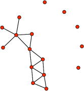
Figure 1: Florentine family business graph.

For this undirected network we propose to estimate the following 2-dimensional model:

$$\pi(\hbox{\boldmath$y$}|\hbox{\boldmath$\theta$})=\frac{1}{z(\hbox{\boldmath$\theta$})}\exp\left\{\theta_{1}s_{1}(\hbox{\boldmath$y$})+\theta_{2}s_{2}(\hbox{\boldmath$y$})\right\}$$ (5)

with statistics $s_{1}(\hbox{\boldmath$y$})=\sum_{i<j}y_{ij}$ and $s_{2}(\hbox{\boldmath$y$})=\sum_{i<j<k}y_{ik}y_{jk}$ which are respectively the observed number of edges and two-stars, that is, the number of nodes with degree at least two. We use the statnet package (Handcock et al., 2007a) in the R programming language to compute estimates of the maximum pseudolikelihood estimator and the Markov chain Monte Carlo estimator. Despite its simplicity the parameters of this model turn out to be difficult to estimate in practice, and both the MPLE and the MC-MLE fail to produce reasonable estimates. Table 1 reports the parameter estimates of both MPLE and MC-MLE. The standard errors of the MC-MLE are unreasonably large due to poor convergence of the algorithm. In fact, in this case it turns out that graphs $\hbox{\boldmath$y$}_{1},\dots,\hbox{\boldmath$y$}_{m}$ simulated from $\pi(\hbox{\boldmath$y$}|\hbox{\boldmath$\theta$}_{0})$, which are used in (4), are typically complete graphs. This is illustrated in Figure 2. The left-hand plots show the trace of the MCMC sampled sufficient statistics simulated during the MCMC iterations, where $\hbox{\boldmath$\theta$}_{0}$ is set equal to the MPLE. The right-hand plots show the respective density estimate. These parameter estimates generate mainly full graphs. This is good evidence of degeneracy, thereby illustrating, in this example, that MPLE and MC-MLE do not give parameter estimates which are in agreement with the observed data.

	MC-MLE		MPLE
Parameter	Estimate	Std. Error	Estimate	Std. Error
$\theta_{1}$ (edges)	-3.39	21.69	-3.39	0.70
$\theta_{2}$ (2-stars)	0.30	0.79	0.35	0.14

Table 1: Summary of parameter estimates of the model (5).

Figure 2: MCMC output of the graphs simulated from (5) where $\hbox{\boldmath$\theta$}_{0}$ is the maximum pseudolikelihood estimate. The top and bottom rows corresponds to $s_{1}(\hbox{\boldmath$y$})$ and $s_{2}(\hbox{\boldmath$y$})$, respectively.

As before, the issue of choice of initial value $\hbox{\boldmath$\theta$}_{0}$ is crucial to the performance and convergence of MC-MLE. In Figure 3 it can be observed how $w_{\hbox{\boldmath$\theta$}_{0}}(\hbox{\boldmath$\theta$})$ in (4) varies with respect to two possible choices of $\hbox{\boldmath$\theta$}_{0}$. In this case note that when $\hbox{\boldmath$\theta$}_{0}$ corresponds to the MPLE, (4) gives an approximation that cannot even be maximized whereas $\hbox{\boldmath$\theta$}_{0}=(0,0)$, for example, would seem to be a better choice.

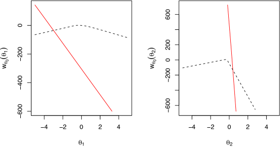
Figure 3: Approximation of the log ratio in (4) by using $w_{\hbox{\boldmath$\theta$}_{0}}(\hbox{\boldmath$\theta$})$ for two different initial values: $\hbox{\boldmath$\theta$}_{0}=\;\mbox{MPLE}$ (solid curve) and $\hbox{\boldmath$\theta$}_{0}=(0,0)$ (dotted curve).

4 Bayesian inference

Consider the Bayesian treatment of this problem (see Koskinen (2004)), where a prior distribution $\pi(\hbox{\boldmath$\theta$})$ is placed on $\theta$, and interest is in the posterior distribution

$$\pi(\hbox{\boldmath$\theta$}|\hbox{\boldmath$y$})\propto\pi(\hbox{\boldmath$y$}|\hbox{\boldmath$\theta$})\pi(\hbox{\boldmath$\theta$}).$$

This type of posterior distribution is sometimes called “doubly-intractable” due to the (standard) intractability of sampling directly from the posterior distribution, but also due to the intractability of the likelihood model within the posterior.

A naïve implementation of a Metropolis-Hastings algorithm proposing to move from $\theta$ to $\hbox{\boldmath$\theta$}^{\prime}$ would require calculation of the following ratio at each sweep of the algorithm

$$\frac{q_{\hbox{\boldmath$\theta$}^{\prime}}(\hbox{\boldmath$y$})\pi(\hbox{\boldmath$\theta$}^{\prime})}{q_{\hbox{\boldmath$\theta$}}(\hbox{\boldmath$y$})\pi(\hbox{\boldmath$\theta$})}\times\frac{z(\hbox{\boldmath$\theta$})}{z(\hbox{\boldmath$\theta$}^{\prime})}$$ (6)

which is unworkable due to the presence of the normalising constants $z(\hbox{\boldmath$\theta$})$ and $z(\hbox{\boldmath$\theta$}^{\prime})$.

4.1 The exchange algorithm

There has been considerable recent activity on the problem of sampling from such complicated distributions, for example, Møller et al. (2006). The algorithm presented in this paper overcomes the problem of sampling from a distribution with intractable normalising constant, to a large extent. However the algorithm can result in an MCMC chain with poor mixing among the parameters. In social network analysis, further developments of this approach have been proposed in Koskinen (2008) and Koskinen et al. (2009) by introducing the linked importance sampler auxiliary variable (LISA) algorithm which employs an importance sampler in each iteration to estimate the acceptance probability.

In this paper we adapt to the ERGMs context the simple and easy-to-implement exchange algorithm presented in Murray et al. (2006). The algorithm samples from an augmented distribution

$$\pi(\hbox{\boldmath$\theta$}^{\prime},\hbox{\boldmath$y$}^{\prime},\hbox{\boldmath$\theta$}|\hbox{\boldmath$y$})\propto\pi(\hbox{\boldmath$y$}|\hbox{\boldmath$\theta$})\pi(\hbox{\boldmath$\theta$})h(\hbox{\boldmath$\theta$}^{\prime}|\hbox{\boldmath$\theta$})\pi(\hbox{\boldmath$y$}^{\prime}|\hbox{\boldmath$\theta$}^{\prime})$$ (7)

where $\pi(\hbox{\boldmath$y$}^{\prime}|\hbox{\boldmath$\theta$}^{\prime})$ is the same distribution as the original distribution on which the data $y$ is defined. The distribution $h(\hbox{\boldmath$\theta$}^{\prime}|\hbox{\boldmath$\theta$})$ is any arbitrary distribution for the augmented variables $\hbox{\boldmath$\theta$}^{\prime}$ which might depend on the variables $\theta$, for example, a random walk distribution centered at $\theta$. It is clear that the marginal distribution for $\theta$ in (7) is the posterior distribution of interest. The algorithm can be written in the following concise way:

1. Gibbs update of $(\hbox{\boldmath$\theta$}^{\prime},\hbox{\boldmath$y$}^{\prime})$:
i Draw $\hbox{\boldmath$\theta$}^{\prime}\sim h(\cdot|\hbox{\boldmath$\theta$})$.
ii Draw $\hbox{\boldmath$y$}^{\prime}\sim\pi(\cdot|\hbox{\boldmath$\theta$}^{\prime})$.

2. Propose the exchange move from $\theta$ to $\hbox{\boldmath$\theta$}^{\prime}$ with probability

$$\alpha=\min\left(1,\frac{q_{\hbox{\boldmath$\theta$}}(\hbox{\boldmath$y$}^{\prime})\pi(\hbox{\boldmath$\theta$}^{\prime})h(\hbox{\boldmath$\theta$}|\hbox{\boldmath$\theta$}^{\prime})q_{\hbox{\boldmath$\theta$}^{\prime}}(\hbox{\boldmath$y$})}{q_{\hbox{\boldmath$\theta$}}(\hbox{\boldmath$y$})\pi(\hbox{\boldmath$\theta$})h(\hbox{\boldmath$\theta$}^{\prime}|\hbox{\boldmath$\theta$})q_{\hbox{\boldmath$\theta$}^{\prime}}(\hbox{\boldmath$y$}^{\prime})}\times\frac{z(\hbox{\boldmath$\theta$})z(\hbox{\boldmath$\theta$}^{\prime})}{z(\hbox{\boldmath$\theta$})z(\hbox{\boldmath$\theta$}^{\prime})}\right).$$ (8)

Notice in step 2, that all intractable normalising constants cancel above and below the fraction. In practice, the exchange move proposes to offer the observed data $y$ the auxiliary parameter $\hbox{\boldmath$\theta$}^{\prime}$ and similarly to offer the auxiliary data $\hbox{\boldmath$y$}^{\prime}$ the parameter $\theta$. The affinity between $\theta$ and $\hbox{\boldmath$y$}^{\prime}$ is measured by $q_{\hbox{\boldmath$\theta$}}(\hbox{\boldmath$y$}^{\prime})/q_{\hbox{\boldmath$\theta$}}(\hbox{\boldmath$y$})$ and the affinity between $\hbox{\boldmath$\theta$}^{\prime}$ and $y$ by $q_{\hbox{\boldmath$\theta$}^{\prime}}(\hbox{\boldmath$y$})/q_{\hbox{\boldmath$\theta$}^{\prime}}(\hbox{\boldmath$y$}^{\prime})$. The difficult step of the algorithm is 1.ii since this requires a draw from $\pi(\hbox{\boldmath$y$}^{\prime}|\hbox{\boldmath$\theta$}^{\prime})$. Note that perfect sampling (Propp and Wilson (1996)) is often possible for Markov random field models, however a pragmatic alternative is to sample from $\pi(\hbox{\boldmath$y$}^{\prime}|\hbox{\boldmath$\theta$}^{\prime})$ by standard MCMC methods, for example, Gibbs sampling, and take a realisation from a long run of the chain as an approximate draw from the distribution. If we suppose that the proposal density $h(\cdot)$ is symmetric, then we can write the acceptance ratio $\alpha$ in (8) as

$$\alpha=\min\left(1,\frac{q_{\hbox{\boldmath$\theta$}^{\prime}}(\hbox{\boldmath$y$})\pi(\hbox{\boldmath$\theta$}^{\prime})q_{\hbox{\boldmath$\theta$}}(\hbox{\boldmath$y$}^{\prime})}{q_{\hbox{\boldmath$\theta$}}(\hbox{\boldmath$y$})\pi(\hbox{\boldmath$\theta$})q_{\hbox{\boldmath$\theta$}^{\prime}}(\hbox{\boldmath$y$}^{\prime})}\right).$$

Comparing this to (6), we see that $q_{\hbox{\boldmath$\theta$}}(\hbox{\boldmath$y$}^{\prime})/q_{\hbox{\boldmath$\theta$}^{\prime}}(\hbox{\boldmath$y$}^{\prime})$ can be thought of as an importance sampling estimate of the ratio $z(\hbox{\boldmath$\theta$})/z(\hbox{\boldmath$\theta$}^{\prime})$ since

$${\mathbb{E}}_{\hbox{\boldmath$y$}^{\prime}|\hbox{\boldmath$\theta$}^{\prime}}\frac{q_{\hbox{\boldmath$\theta$}}(\hbox{\boldmath$y$}^{\prime})}{q_{\hbox{\boldmath$\theta$}^{\prime}}(\hbox{\boldmath$y$}^{\prime})}=\sum_{\hbox{\boldmath$y$}}\frac{q_{\hbox{\boldmath$\theta$}}(\hbox{\boldmath$y$}^{\prime})}{q_{\hbox{\boldmath$\theta$}^{\prime}}(\hbox{\boldmath$y$}^{\prime})}\frac{q_{\hbox{\boldmath$\theta$}^{\prime}}(\hbox{\boldmath$y$}^{\prime})}{z(\hbox{\boldmath$\theta$}^{\prime})}=\frac{z(\hbox{\boldmath$\theta$})}{z(\hbox{\boldmath$\theta$}^{\prime})}.$$

Recall that this is the identity (3) used in the Geyer-Thompson method. Note that this algorithm has some similarities with another likelihood-free method called Approximate Bayesian Computation (ABC) (see Beaumont et al. (2002) and Marjoram et al. (2003)). The ABC algorithm also relies on drawing parameter values $\hbox{\boldmath$\theta$}^{\prime}$ and simulating new graphs from those values. The proposed move is accepted if there is good agreement between auxiliary data and observed data in terms of summary statistics. Here a good approximation to the true posterior density is guaranteed by the fact that the summary statistics are sufficient statistics of the probability model.

4.2 MCMC simulation from ERGMs

Recall that step 1.ii of the exchange algorithm requires a draw $\hbox{\boldmath$y$}^{\prime}$ from $\pi(\hbox{\boldmath$y$}^{\prime}|\hbox{\boldmath$\theta$})$. The simulation of a network given a parameter value is accomplished by an MCMC algorithm which at each iteration compares the probability of a proposed graph to the observed one and then decides whether or not accept the proposed network. The latter is selected at each step by proposing a change in the current state of a single dyad (i.e. creating a new edge or dropping an old edge). This is obviously a computationally intensive procedure.
In order to improve mixing of the Markov chain the ergm package for R (Hunter et al., 2008) uses by default the “tie no tie” (TNT) sampler. This is the approach we take throughout this paper. At each iteration of the chain the TNT sampler, instead of selecting a dyad at random, first selects with equal probability the set of edges or the set of empty dyads, and than swaps a dyad at random within that chosen set. In this way, since most of the realistic networks are quite sparse, the probability of selecting an empty dyad to swap is lower and the sampler does not waste too much time proposing new edges which are likely to be rejected (Morris et al., 2008). Moreover, initialising the auxiliary chain with the observed network $y$ leads to improved efficiency in terms of acceptance rates. This is the default choice in our implementation of the algorithm, which we now describe.

4.3 Implementing the algorithm

The exchange algorithm can be easily implemented by using existing software and the ergm package is particularly appropriate for this purpose. An R package called Bergm, which accompanies this paper, draws heavily on the ergm package and provides functions for the implementation of the exchange algorithm which have been used to obtain the results reported in this paper.

Let us return to the running example from Section 3.4. The posterior distribution of model (5) is written as

$$\pi(\hbox{\boldmath$\theta$}|\hbox{\boldmath$y$})\propto\frac{1}{z(\hbox{\boldmath$\theta$})}\exp\left\{\theta_{1}\sum_{i<j}y_{ij}+\theta_{2}\sum_{i<j<k}y_{ik}y_{jk}\right\}\pi(\hbox{\boldmath$\theta$}).$$ (9)

Here we assume a flat multivariate normal prior $\pi(\hbox{\boldmath$\theta$})\sim\mathcal{N}(\mathbf{0},30\hbox{\boldmath$I$}_{d})$ where $\hbox{\boldmath$I$}_{d}$ is the identity matrix of size equal to the number of model dimensions $d$. The simplest approach to update the parameter state is to update its components one at a time, using a single-site update sampler. We use the following proposals for the first and the second parameter value, respectively, $h(\cdot|\theta_{1})\sim\mathcal{N}(0,1)$ and $h(\cdot|\theta_{2})\sim\mathcal{N}(0,0.1)$ where the proposal tuning parameters are chosen in order to reach a reasonable level of mixing, in this case an overall acceptance rate of $18\%$. The auxiliary chain consists of $1,000$ iterations and the main one of $30,000$ iterations.
The posterior estimates are reported in Table 2. From Figure 4 it can be seen that the estimates produced by the exchange algorithm are very different from the ones obtained by MC-MLE and MPLE. The autocorrelation plots show that the autocorrelations are negligible after lag 150.

Figure 4: MCMC output of the pedagogical model (9).

As mentioned in Section 4.1, an important issue for implementation of this algorithm is that of drawing from $\pi(\hbox{\boldmath$y$}^{\prime}|\hbox{\boldmath$\theta$}^{\prime})$ and a pragmatic way to do that is to use the final realisation of a graph simulated from a long run of an MCMC sampler. Here we are interested in testing the sensitivity of the posterior output to the number of auxiliary iterations used to generate the sampled graph. Table 2 displays the results using three different number of iterations for the auxiliary chain. As we can see from the three outputs, there is not a significant difference between the results obtained using $500$ or more iterations.

Iterations	Parameter	Post. Mean	Post. Sd.
$500$	$\theta_{1}$ (edges)	-2.43	0.52
	$\theta_{2}$ (2-stars)	0.11	0.12
$1,000$	$\theta_{1}$ (edges)	-2.42	0.51
	$\theta_{2}$ (2-stars)	0.11	0.11
$5,000$	$\theta_{1}$ (edges)	-2.43	0.51
	$\theta_{2}$ (2-stars)	0.10	0.12

Table 2: Posterior outputs for different numbers of iterations for the auxiliary chain.

It is worth mentioning here that the posterior density is highly correlated and that the high posterior density region is thin. The high posterior density region for the pedagogical example is shown in the left-hand plot of Figure 5. In such a situation, which is not rare for these kind of models, in absence of any information about the covariance structure of the posterior distribution, the single-site update may not be the best procedure as it may result in a poorly mixing MCMC sampler. We will discuss this issue in Section 4.5.

4.4 Convergence of the Markov chain

Exploration of the parameters of the posterior distribution using MCMC is of crucial importance, but more so in light of the problem of degeneracy. Here we have that, to a large extent, the exchange algorithm results in quite fast convergence to the stationary distribution. We present a heuristic argument as to why this is the case. Assume that $s(\hbox{\boldmath$y$})\in rint(C)$, that $\pi(\hbox{\boldmath$\theta$})$ is very flat and that $h(\cdot)$ is symmetric. We can then write the acceptance ratio (8) as:

$$\alpha\approx\min\left(1,\exp\left\{(\hbox{\boldmath$\theta$}-\hbox{\boldmath$\theta$}^{\prime})^{t}(s(\hbox{\boldmath$y$}^{\prime})-s(\hbox{\boldmath$y$}))\right\}\right)$$ (10)

where $s(\hbox{\boldmath$y$})$ is the fixed vector of the sufficient statistics of the observed graph and $s(\hbox{\boldmath$y$}^{\prime})$ is a vector of sufficient statistics of a graph drawn from $\pi(\hbox{\boldmath$y$}^{\prime}|\hbox{\boldmath$\theta$}^{\prime})$. It is known, see Section 2 of van Duijn et al. (2009), for example, that

$$(\hbox{\boldmath$\theta$}-\hbox{\boldmath$\theta$}^{\prime})^{t}(\mu(\hbox{\boldmath$\theta$})-\mu(\hbox{\boldmath$\theta$}^{\prime}))\geq 0.$$ (11)

Recall that $\mu(\hbox{\boldmath$\theta$})={\mathbb{E}}_{\hbox{\boldmath$\theta$}}[s(\hbox{\boldmath$y$})]$ is the mean parameterisation for $\theta$. Notice that if there is good agreement between $y$ and $\hbox{\boldmath$\theta$}^{\prime}$, and good agreement between $\hbox{\boldmath$y$}^{\prime}$ and $\theta$, then

$$s(\hbox{\boldmath$y$}^{\prime})\approx\mu(\hbox{\boldmath$\theta$})\;\;\mbox{and}\;\;s(\hbox{\boldmath$y$})\approx\mu(\hbox{\boldmath$\theta$}^{\prime}).$$

Equation (11) would then implies that the exponent in (10) is positive, whereby the exchange move is accepted. Empirically, it has been observed that fast convergence occurs even when the initial parameters are set to lie in the degenerate region. The right-hand plot of Figure 5 displays the two dimensional trace of 12 MCMC runs starting from very different points in the parameter space for the pedagogical example. In each instance, the Markov chain converges quickly to the high posterior density region. In fact, we have observed this behaviour for each of the datasets we analysed.

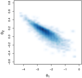
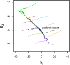
Figure 5: Posterior density (left) and traces (right) of the first $1,000$ iterations of 12 chains from the posterior distribution corresponding to the pedagogical example.

Recall that the exchange algorithm involves drawing networks from the likelihood model. It is natural to ask questions such as, what proportion of such simulated networks are full or empty? And more importantly are any of these networks accepted in the MCMC algorithm? Figure 6 partly answers these questions, in the case of the pedagogical example of Section 3.4. Here it can be seen that the algorithm frequently simulates low or high density graphs, but most of the networks accepted are those whose sufficient statistics are in close agreement to the observed sufficient statistics. This is a very useful aspect of the algorithm.

Figure 6: Number of edges (left) and two-stars (right) of $2,000$ graphs (thinned by a factor of 15 from the original $30,000$ iterations) simulated (gray dots) and graphs whose parameters were accepted (black dots). The solid line represents the number of edges in the observed graph.

4.5 Population MCMC can improve mixing

While easy to implement, the single-site update procedure can lead to slow mixing if there is strong temporal dependence in the state process. As shown above, often there may be a strong correlation between model parameters and also the high posterior density region can be thin. In order to improve mixing we propose to use an adaptive direction sampling (ADS) method (Gilks et al. (1994) and Roberts and Gilks (1994)), similar to that of ter Braak and Vrugt (2008). We consider a population MCMC approach consisting of a collection of $H$ chains which interact with one another. Here the state space is $\{\hbox{\boldmath$\theta$}_{1},\dots,\hbox{\boldmath$\theta$}_{H}\}$ with target distribution $\pi(\hbox{\boldmath$\theta$}_{1}|\hbox{\boldmath$y$})\otimes\cdots\otimes\pi(\hbox{\boldmath$\theta$}_{H}|\hbox{\boldmath$y$})$. A ”parallel ADS” move may be described algorithmically as follows.

• For each chain $h=1,\dots,H$

  • Select at random $h_{1}$ and $h_{2}$ without replacement from $\{1,\dots,H\}\setminus h$

  • Sample $\epsilon$ from a symmetric distribution

  • Propose $\hbox{\boldmath$\theta$}^{\prime}_{h}=\hbox{\boldmath$\theta$}^{i}_{h}+\gamma\left(\hbox{\boldmath$\theta$}^{i}_{h_{1}}-\hbox{\boldmath$\theta$}^{i}_{h_{2}}\right)+\hbox{\boldmath$\epsilon$}$

  • Sample $\hbox{\boldmath$y$}^{\prime}$ from $\pi(\cdot|\hbox{\boldmath$\theta$}^{\prime}_{h})$ by MCMC methods, for example, the “tie no tie” (TNT) sampler, taking a realisation from a long run of the chain as an approximate draw from this distribution.

  • Accept the move from $\hbox{\boldmath$\theta$}^{i}_{h}$ to $\hbox{\boldmath$\theta$}^{i+1}_{h}=\hbox{\boldmath$\theta$}^{\prime}_{h}$ with probability

    $$\alpha=\min\left(1,\frac{q_{\hbox{\boldmath$\theta$}^{i}_{h}}(\hbox{\boldmath$y$}^{\prime})\pi(\hbox{\boldmath$\theta$}^{\prime}_{h})q_{\hbox{\boldmath$\theta$}^{\prime}_{h}}(\hbox{\boldmath$y$})}{q_{\hbox{\boldmath$\theta$}^{i}_{h}}(\hbox{\boldmath$y$})\pi(\hbox{\boldmath$\theta$}^{i}_{h})q_{\hbox{\boldmath$\theta$}^{\prime}_{h}}(\hbox{\boldmath$y$}^{\prime})}\right).$$

This move is illustrated graphically in Figure 7.

Figure 7: (a) The parallel ADS move of $\hbox{\boldmath$\theta$}^{i}_{h}$ is generated from the difference of the states $\hbox{\boldmath$\theta$}^{i}_{h_{1}}$ and $\hbox{\boldmath$\theta$}^{i}_{h_{2}}$ selected from the other chains and a random term $\epsilon$. (b) The reverse jump is obtained by reversing $\epsilon$ and the order of the difference between $\hbox{\boldmath$\theta$}^{i}_{h_{1}}$ and $\hbox{\boldmath$\theta$}^{i}_{h_{2}}$.

For our running example we set $\gamma=1$ and $\hbox{\boldmath$\epsilon$}\sim\mathcal{N}(\mathbf{0},0.1\hbox{\boldmath$I$}_{d})$ where the tuning parameters were set so that the acceptance rate is around $20\%$. Initially all the chains are run in parallel using a block update of each individual chain and after a certain number of iterations the parallel ADS update begins. For this example we set the number of chains $H=5$. The posterior output from the population MCMC algorithm is shown in Table 3.

	Parameter	Post. Mean	Post. Sd.
Chain 1	$\theta_{1}$ (edges)	-2.39	0.55
	$\theta_{2}$ (2-stars)	0.11	0.12
Chain 2	$\theta_{1}$ (edges)	-2.49	0.51
	$\theta_{2}$ (2-stars)	0.13	0.12
Chain 3	$\theta_{1}$ (edges)	-2.43	0.57
	$\theta_{2}$ (2-stars)	0.11	0.12
Chain 4	$\theta_{1}$ (edges)	-2.44	0.54
	$\theta_{2}$ (2-stars)	0.13	0.13
Chain 5	$\theta_{1}$ (edges)	-2.42	0.52
	$\theta_{2}$ (2-stars)	0.12	0.13
Overall	$\theta_{1}$ (edges)	-2.44	0.54
	$\theta_{2}$ (2-stars)	0.12	0.12

Table 3: Summary of posterior parameter density of the model (9).

Figure 8 shows that the autocorrelation curve now decreases faster than the single-site update algorithm and is negligible at around lag 50. Recall that for the single-site update version of this algorithm, the autocorrelation is negligible after lag $150$. Therefore the single-site sampler would need to be run for around $3$ times more iterations than the population MCMC sampler in order to achieve a comparable number of effectively independent draws from the posterior distribution. For more complex networks, the reduction in autocorrelation using the population MCMC algorithm was considerable.

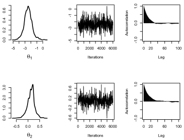
Figure 8: MCMC output of a single chain of the model (9).

Figure 9 depicts the 2-dimensional trace of 400 iterations for both the single-site update and a single chain using the parallel ADS update. We see that the latter can easily move into the correlated high posterior density region thus ensuring a better mixing of the algorithm.

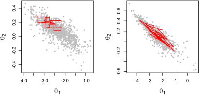
Figure 9: 2-D traces of 400 iterations for the single-site update algorithm (left) and a single chain of the parallel ADS update algorithm (right).

The algorithm took approximately 13 minutes to estimate model (9) using $30,000$ iterations of the single-site update and about 6 minutes using the parallel ADS updater with $6,000$ iterations per chain.

5 Examples

We now consider three different benchmark networks datasets (two undirected and one directed) and we illustrate models with various specifications (see Robins et al. (2007a) and Snijders et al. (2006) for details). For each of them we apply the population MCMC with parallel ADS update, setting the number of chains equal to twice the number of model parameters.

5.1 Molecule synthetic network

This dataset is included with the ergm package for R. The elongated shape of this 20-node graph, shown in Figure 10, resembles the chemical structure of a molecule.

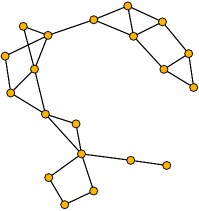
Figure 10: Molecule synthetic graph.

We consider the following 4-dimensional model

$$\pi(\hbox{\boldmath$\theta$}|\hbox{\boldmath$y$})\propto\frac{1}{z(\hbox{\boldmath$\theta$})}\exp\left\{\sum_{i=1}^{4}\theta_{i}s_{i}(\hbox{\boldmath$y$})\right\}\pi(\hbox{\boldmath$\theta$})$$ (12)

where

$s_{1}(\hbox{\boldmath$y$})=\sum_{i<j}y_{ij}$	number of edges
$s_{2}(\hbox{\boldmath$y$})=\sum_{i<j<k}y_{ik}y_{jk}$	number of two-stars
$s_{3}(\hbox{\boldmath$y$})=\sum_{i<j<k<l}y_{il}y_{jl}y_{kl}$	number of three-stars
$s_{4}(\hbox{\boldmath$y$})=\sum_{i<j<k}y_{jk}y_{ik}y_{ij}$	number of triangles

We use the flat prior $\pi(\theta_{i})\sim\mathcal{N}(0,30)$, for $i=1,\dots,4$, and we set $\gamma=0.5$ and $\hbox{\boldmath$\epsilon$}\sim\mathcal{N}(\mathbf{0},0.1\hbox{\boldmath$I$})$ corresponding to an overall acceptance probability of $22\%$. The auxiliary chain consists of $1,000$ iterations and the main one of $4,000$ iterations for each chain. The algorithm took approximately 9 minutes to sample the posterior model (12) for a total of $32,000$ iterations. In Table 4 we see that the posterior density estimates of the 8 chains are similar to each other. Aggregating the output across all chains, the posterior estimates for the first three parameters indicate an overall tendency for nodes to have a limited number of multiple edges while the positive estimates relative to the triangle parameter capture the propensity towards transitivity. Table 5 reports the estimates of both MC-MLE and MPLE. Here MC-MLE fails to converge as the MPLE estimates generate mainly full graphs.

In Figure 11 it can be seen that the autocorrelations of the parameters decay quickly around lag $200$. By comparison, a single chain sampler (not reported here) with single-site updating of the $\theta$ vector led to negligible autocorrelation at around lag $1,000$. Therefore, the single-site sampler would need to be run for around $5$ times more iterations than the population MCMC sampler in order to achieve comparable number of effectively independent draws from the posterior distribution.

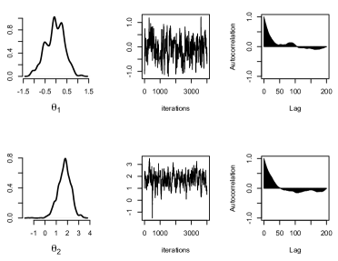
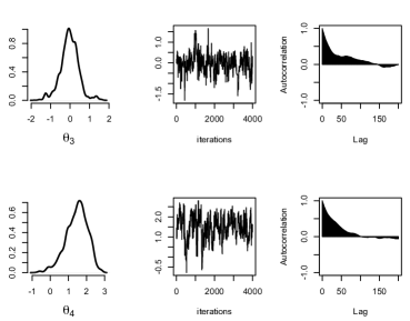
Figure 11: Molecule dataset: MCMC output of a single chain of the posterior distribution (12).

	Parameter	Post. Mean	Post. Sd.
Chain 1	$\theta_{1}$ (edges)	2.88	3.10
	$\theta_{2}$ (2-stars)	-1.06	0.92
	$\theta_{3}$ (3-stars)	-0.04	0.43
	$\theta_{4}$ (triangles)	1.55	0.54
Chain 2	$\theta_{1}$ (edges)	2.61	3.12
	$\theta_{2}$ (2-stars)	-1.02	0.99
	$\theta_{3}$ (3-stars)	-0.05	0.42
	$\theta_{4}$ (triangles)	1.70	0.57
Chain 3	$\theta_{1}$ (edges)	2.71	3.13
	$\theta_{2}$ (2-stars)	-1.01	0.96
	$\theta_{3}$ (3-stars)	-0.06	0.48
	$\theta_{4}$ (triangles)	1.58	0.53
Chain 4	$\theta_{1}$ (edges)	2.68	3.35
	$\theta_{2}$ (2-stars)	-1.01	1.02
	$\theta_{3}$ (3-stars)	-0.03	0.47
	$\theta_{4}$ (triangles)	1.45	0.59
Chain 5	$\theta_{1}$ (edges)	2.72	3.11
	$\theta_{2}$ (2-stars)	-1.10	1.14
	$\theta_{3}$ (3-stars)	-0.02	0.44
	$\theta_{4}$ (triangles)	1.59	0.63
Chain 6	$\theta_{1}$ (edges)	2.87	3.46
	$\theta_{2}$ (2-stars)	-1.05	1.00
	$\theta_{3}$ (3-stars)	-0.10	0.47
	$\theta_{4}$ (triangles)	1.65	0.55
Chain 7	$\theta_{1}$ (edges)	2.60	3.25
	$\theta_{2}$ (2-stars)	-1.10	1.06
	$\theta_{3}$ (3-stars)	-0.10	0.47
	$\theta_{4}$ (triangles)	1.62	0.51
Chain 8	$\theta_{1}$ (edges)	2.82	3.64
	$\theta_{2}$ (2-stars)	-1.03	1.03
	$\theta_{3}$ (3-stars)	-0.10	0.50
	$\theta_{4}$ (triangles)	1.61	0.59
Overall	$\theta_{1}$ (edges)	2.72	3.27
	$\theta_{2}$ (2-stars)	-1.02	1.02
	$\theta_{3}$ (3-stars)	-0.05	0.46
	$\theta_{4}$ (triangles)	1.60	0.57

Table 4: Molecule dataset: summary of posterior parameter density of the molecule network (12).

	MC-MLE		MPLE
Parameter	Estimate	Std. Error	Estimate	Std. Error
$\theta_{1}$ (edges)	4.11	NA	5.08	1.90
$\theta_{2}$ (2-stars)	-1.64	NA	-2.02	0.60
$\theta_{3}$ (3-stars)	0.42	NA	0.52	0.27
$\theta_{4}$ (triangles)	1.30	NA	1.60	0.39

Table 5: Molecule dataset: Summary of parameter estimates of the model (12).

A pragmatic way to examine the fit of the data to the posterior model the output obtained is to implement a Bayesian goodness-of-fit procedure. In order to do this, 100 graphs are simulated from 100 independent realisations taken from the estimated posterior distribution and compared to the observed graph in terms of high-level characteristics which are not modelled explicitly, namely, degree distributions (for degrees greater than 3); the minimum geodesic distance (namely, the proportion of pairs of nodes whose shortest connected path is of length $l$, for $l=1,2,\dots$); the number of edge-wise shared partners (the number of edges in the network that share $l$ neighbours in common for $l=1,2,\dots$.) The results are shown in Figure 12 and indicate that the structure of the observed graph can be considered as a possible realisation of the posterior density.

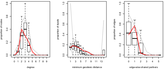
Figure 12: Molecule dataset: Bayesian goodness-of-fit output.

5.2 Dolphins network

The undirected graph displayed in Figure 13 represents social associations between 62 dolphins living off Doubtfull Sound in New Zealand (Lusseau et al., 2003). The graph is inhomogeneous, a few nodes have large number of edges and many have only one or two edges.

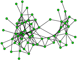
Figure 13: Dolphins network dataset.

We propose to estimate the following 3-dimensional model using three new specifications proposed by Snijders et al. (2006):

$$\pi(\hbox{\boldmath$\theta$}|\hbox{\boldmath$y$})\propto\frac{1}{z(\hbox{\boldmath$\theta$})}\exp\left\{\theta_{1}s_{1}(\hbox{\boldmath$y$})+\theta_{2}u(\hbox{\boldmath$y$},\phi_{u})+\theta_{3}v(\hbox{\boldmath$y$},\phi_{v})\right\}\pi(\hbox{\boldmath$\theta$})$$ (13)

where

$s_{1}(\hbox{\boldmath$y$})=\sum_{i<j}y_{ij}$	number of edges
$u(\hbox{\boldmath$y$},\phi_{u})=e^{\phi_{u}}\sum_{i=1}^{n-1}\left\{1-\left(1-e^{-\phi_{u}}\right)^{i}\right\}D_{i}(\hbox{\boldmath$y$})$	geometrically weighted degree
$v(\hbox{\boldmath$y$},\phi_{v})=e^{\phi_{v}}\sum_{i=1}^{n-2}\left\{1-\left(1-e^{-\phi_{v}}\right)^{i}\right\}EP_{i}(\hbox{\boldmath$y$})$	geometrically weighted edgewise
	shared partner.

We set $\phi_{u}=0.8$ and $\phi_{v}=0.8$ so that the model is a regular, that is, a non-curved exponential random graph model (Hunter and Handcock, 2006). We use the flat multivariate normal prior $\pi(\hbox{\boldmath$\theta$})\sim\mathcal{N}(\mathbf{0},30\hbox{\boldmath$I$})$ and we set $\gamma=0.5$ and $\hbox{\boldmath$\epsilon$}\sim\mathcal{N}(\mathbf{0},0.1\hbox{\boldmath$I$})$, where the tuning parameters were chosen so that the overall acceptance rate was around $10\%$. The auxiliary chain consists of $15,000$ iterations and the main chain $10,000$ iterations for each of the 6 chains of the population. The algorithm took approximately 1 hour and 10 minutes to estimate model (13). A single-site algorithm would take many more hours to carry out estimation using the same overall number of iterations. From Table 6 it can seen that mixing across the chains appears to be reasonable and the overall posterior estimates displayed in the lower block of Table 6 provide us with a useful interpretation of the observed graph. The tendency to a low density of edges expressed by the negative posterior mean of the first parameter, is balanced by a propensity to multiple local clustering and tied nodes to share multiple neighbours in common expressed, respectively, by the last two positive posterior parameter estimates.

	Parameter	Post. Mean	Post. Sd.
Chain 1	$\theta_{1}$ (edges)	-4.24	0.32
	$\theta_{2}$ (gwd)	1.28	0.50
	$\theta_{3}$ (gwesp)	0.94	0.13
Chain 2	$\theta_{1}$ (edges)	-4.24	0.34
	$\theta_{2}$ (gwd)	1.27	0.50
	$\theta_{3}$ (gwesp)	0.94	0.13
Chain 3	$\theta_{1}$ (edges)	-4.27	0.33
	$\theta_{2}$ (gwd)	1.32	0.50
	$\theta_{3}$ (gwesp)	0.95	0.13
Chain 4	$\theta_{1}$ (edges)	-4.27	0.35
	$\theta_{2}$ (gwd)	1.27	0.52
	$\theta_{3}$ (gwesp)	0.95	0.13
Chain 5	$\theta_{1}$ (edges)	-4.30	0.37
	$\theta_{2}$ (gwd)	1.32	0.55
	$\theta_{3}$ (gwesp)	0.95	0.13
Chain 6	$\theta_{1}$ (edges)	-4.24	0.34
	$\theta_{2}$ (gwd)	1.32	0.51
	$\theta_{3}$ (gwesp)	0.95	0.13
Overall	$\theta_{1}$ (edges)	-4.27	0.35
	$\theta_{2}$ (gwd)	1.30	0.52
	$\theta_{3}$ (gwesp)	0.95	0.13

Table 6: Dolphins dataset: summary of posterior parameter density of the model (13).

Posterior estimates and autocorrelation function plots are reported in Figure 14. Each of the 3 autocorrelation functions decrease quite quickly and are negligible at around lag 200. A single chain MCMC version of the algorithm (not reported here) led to autocorrelation functions which decayed after lag $1500$ – roughly a $7$ fold increases with respect to the population MCMC version of the algorithm.

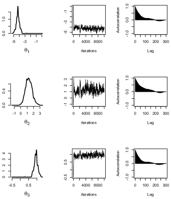
Figure 14: Dolphins dataset: MCMC output of a single chain of the model (13).

As an aside, note that both the MC-MLE and MPLE estimates were quite similar to the posterior mean estimates for this dataset.

Similar to the previous example, we carry out a Bayesian goodness of fit test. The results of this are displayed in Figure 15 and suggest that the model is a reasonable fit to the data.

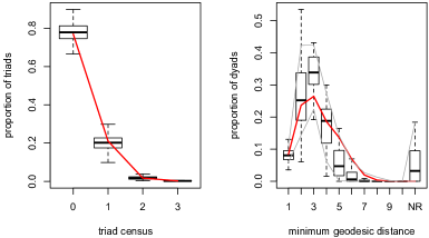
Figure 15: Dolphins dataset: Bayesian goodness-of-fit output.

5.3 Sampson’s Monk network

This network represents the liking relationships among a group of 18 novices who were preparing to join a monastic order (Sampson, 1968). This network consists of directed edges between actors, and is presented in Figure 16.

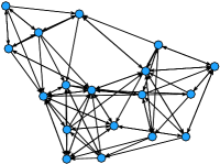
Figure 16: Sampson’s Monk network.

We propose to estimate the following 3-dimensional model

$$\pi(\hbox{\boldmath$\theta$}|\hbox{\boldmath$y$})\propto\frac{1}{z(\hbox{\boldmath$\theta$})}\exp\left\{\theta_{1}s_{1}(\hbox{\boldmath$y$})+\theta_{2}s_{2}(\hbox{\boldmath$y$})+\theta_{3}s_{3}(\hbox{\boldmath$y$})\right\}\pi(\hbox{\boldmath$\theta$})$$ (14)

where

$s_{1}(\hbox{\boldmath$y$})=\sum_{i<j}y_{ij}$	number of edges
$s_{2}(\hbox{\boldmath$y$})=\sum_{i<j}y_{ij}y_{ji}$	number of mutual edges
$s_{3}(\hbox{\boldmath$y$})=\sum_{i<j}y_{ij}y_{jk}y_{ki}$	number of cyclic triads.

We use the flat multivariate normal prior $\pi(\hbox{\boldmath$\theta$})\sim\mathcal{N}(\mathbf{0},30\hbox{\boldmath$I$}_{3})$ and we set $\gamma=0.8$ and $\hbox{\boldmath$\epsilon$}\sim\mathcal{N}(\mathbf{0},0.1\hbox{\boldmath$I$}_{3})$, giving an overall acceptance rate of $18\%$. The auxiliary chain consists of $2,000$ iterations and the main one of $5,000$ iterations for each of the 6 chains of the population. Notice in Table 7 that there is very little difference in output between the chains, giving good evidence that there is reasonable mixing between parameters across the chains. Table 7 shows that the posterior estimate for the cyclic triads parameter is not significative. The tendency to a low number of edges as expressed by the edge parameter is balanced by a high level of reciprocity expressed by mutual parameter.

	Parameter	Post. Mean	Post. Sd.
Chain 1	$\theta_{1}$ (edges)	-1.72	0.31
	$\theta_{2}$ (mutual)	2.34	0.43
	$\theta_{3}$ (ctriple)	-0.05	0.16
Chain 2	$\theta_{1}$ (edges)	-1.73	0.30
	$\theta_{2}$ (mutual)	2.38	0.42
	$\theta_{3}$ (ctriple)	-0.02	0.16
Chain 3	$\theta_{1}$ (edges)	-1.74	0.29
	$\theta_{2}$ (mutual)	2.37	0.43
	$\theta_{3}$ (ctriple)	-0.04	0.15
Chain 4	$\theta_{1}$ (edges)	-1.72	0.29
	$\theta_{2}$ (mutual)	2.33	0.44
	$\theta_{3}$ (ctriple)	-0.06	0.16
Chain 5	$\theta_{1}$ (edges)	-1.73	0.30
	$\theta_{2}$ (mutual)	2.30	0.43
	$\theta_{3}$ (ctriple)	-0.06	0.16
Chain 6	$\theta_{1}$ (edges)	-1.72	0.30
	$\theta_{2}$ (mutual)	2.27	0.44
	$\theta_{3}$ (ctriple)	-0.06	0.16
Overall	$\theta_{1}$ (edges)	-1.72	0.30
	$\theta_{2}$ (mutual)	2.33	0.43
	$\theta_{3}$ (ctriple)	-0.04	0.16

Table 7: Monks dataset: Summary of posterior parameter density of the model (14).

Figure 17 displays posterior density estimates from a single chain of the MCMC algorithm, together with autocorrelation functions for each parameter. All 3 autocorrelation functions decrease quite quickly and are negligible at around lag 60. This behaviour was very similar to each of the other 5 chains. By comparison, a single chain MCMC run (not reported here) with an equivalent number of iterations led to significantly higher autocorrelations, which were negligible at lag $400$. Roughly $6$ or $7$ times more iterations for a single chain run would therefore be needed to yield effectively the same number of independent draws from the posterior as the population MCMC version of the algorithm.

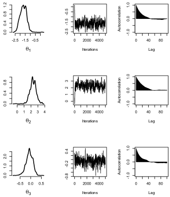
Figure 17: Monks dataset: MCMC output of a single chain from (14).

Here the algorithm took approximately 8 minutes to estimate model (14). As for the previous example, we note that the MC-MLE and MPLE estimates are similar to the posterior mean estimates.

As before, we propose a series of Bayesian goodness-of-fit tests to understand how well the estimated model fits a set of observations. The results in Figure 18 suggest that the model is a reasonable fit to the data. Since the network has directed edges, we used in-degree and out-degree statistics, instead of degree distributions.

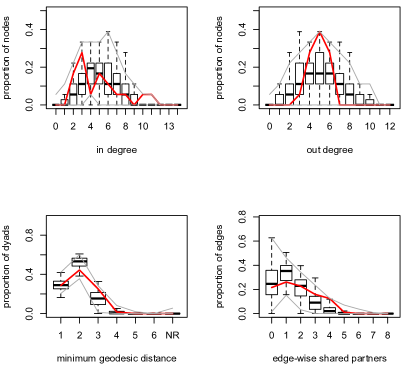
Figure 18: Monks dataset: Bayesian goodness-of-fit output.

6 Discussion

This paper has presented a Bayesian inferential framework for social network analysis for exponential random graph models. The approach used here, based on the exchange algorithm Murray et al. (2006), is shown to give very good performance. Here we present some datasets for which classical inference approaches, Maximum pseudolikelihood estimation and Monte Carlo - Maximum likelihood estimation, both of which are standard practice in social network analysis, fail to give reasonable parameter estimates. By contrast the Bayesian approach yield parameter estimates consistent with the data, in the sense that networks simulated from the posterior had similar topologies to the observed data.

The issue of model degeneracy is important for ERGMs, and one which can cause potential difficulties for inference methods, especially for the MC-MLE method – a poorly chosen set of initial parameters, from the degeneracy region will lead to poor estimation. Empirical evidence presented in this paper, suggests that the method we propose here results in a Markov chain which, even if initialised with parameters from the degenerate region, will quickly converge to the posterior high density regions.

Our analysis has shown that the high posterior density region of ERGMs has typically very thin and correlated support. This point is well addressed in Rinaldo et al. (2009), for example. This presents a very difficult situation for exploration of the posterior support using MCMC methods. The population MCMC method presented in this paper is a useful first step towards addressing this problem, and further exploration in this direction should prove useful. All of the methods used in this paper are presented in the R package Bergm which accompanies this paper, and should prove useful to practitioners.

Estimation for larger networks is feasible but at the cost of increased computational time. In experiments not reported here, we carried out inference for a graph with $104$ nodes in under $2$ hours. Generally speaking, it seems reasonable to expect that the number of iterations needed for the auxiliary chain should be proportional to the number of dyads of the graphs, $n^{2}$ for a graph with $n$ nodes. This is the computational bottleneck of the algorithm. The population MCMC approach which we outlined is very well suited to parallel computing, and this may in turn lead to reduction in the computational time needed to service ERGMs using the algorithm described in this paper.

Acknowledgement

Alberto Ciamo was supported by an IRCSET Embark Initiative award and Nial Friel’s research was supported by a Science Foundation Ireland Research Frontiers Program grant, 09/RFP/MTH2199. The authors wish to acknowledge Johan Koskinen and Michael Schwienberger for helpful comments on an earlier draft of this paper and also to thank the participants of the workshop Statistical Methods for the Analysis of Network Data in Practice in Dublin, June 2009, for useful feedback and constructive comments on this work.

References

- Airoldi et al. (2008) Airoldi, E. M., Blei, D. M., Fienberg, S. E., and Xing, E. P. (2008), “Mixed Membership Stochastic Blockmodels,” Journal of Machine Learning Research, 9, 1981–2014.
- Beaumont et al. (2002) Beaumont, M. A., Zhang, W., and Balding, D. J. (2002), “Approximate Bayesian computation in population genetics,” Genetics, 162, 2025–2035.
- Besag (1974) Besag, J. E. (1974), “Spatial interaction and the statistical analysis of lattice systems (with discussion),” Journal of the Royal Statistical Society, Series B, 36, 192–236.
- Erdös and Rényi (1959) Erdös, P. and Rényi, A. (1959), “On random graphs,” Publicationes Mathematicae, 6, 290–297.
- Frank and Strauss (1986) Frank, O. and Strauss, D. (1986), “Markov Graphs,” Journal of the American Statistical Association, 81, 832–842.
- Friel et al. (2009) Friel, N., Pettitt, A. N., Reeves, R., and Wit, E. (2009), “Bayesian inference in hidden Markov random fields for binary data defined on large lattices,” Journal of Computational and Graphical Statistics, 18, 243–261.
- Geyer and Thompson (1992) Geyer, C. J. and Thompson, E. A. (1992), “Constrained Monte Carlo maximum likelihood for dependent data (with discussion),” Journal of the Royal Statistical Society, Series B, 54, 657–699.
- Gilks et al. (1994) Gilks, W. R., Roberts, G. O., and George, E. I. (1994), “Adaptive direction sampling,” Statistician, 43, 179–189.
- Handcock (2003) Handcock, M. S. (2003), “Assessing Degeneracy in Statistical Models of Social Networks,” Working Paper no.39, Center for Statistics and the Social Sciences, University of Washington.
- Handcock et al. (2007a) Handcock, M. S., Hunter, D. R., Butts, C. T., Goodreau, S. M., and Morris, M. (2007a), “statnet: Software Tools for the Representation, Visualization, Analysis and Simulation of Network Data,” Journal of Statistical Software, 24, 1–11.
- Handcock et al. (2007b) Handcock, M. S., Raftery, A. E., and Tantrum, J. M. (2007b), “Model-based clustering for social networks,” Journal Of The Royal Statistical Society Series A, 170, 301–354.
- Hoff et al. (2002) Hoff, P. D., Raftery, A. E., and Handcock, M. S. (2002), “Latent Space Approaches to Social Network Analysis,” Journal of the American Statistical Association, 97, 1090–1098.
- Holland and Leinhardt (1981) Holland, P. W. and Leinhardt, S. (1981), “An exponential family of probability distributions for directed graphs (with discussion),” Journal of the American Statistical Association, 76, 33–65.
- Hunter and Handcock (2006) Hunter, D. R. and Handcock, M. S. (2006), “Inference in curved exponential family models for networks,” Journal of Computational and Graphical Statistics, 15, 565–583.
- Hunter et al. (2008) Hunter, D. R., Handcock, M. S., Butts, C. T., Goodreau, S. M., and Morris, M. (2008), “ergm: A Package to Fit, Simulate and Diagnose Exponential-Family Models for Networks,” Journal of Statistical Software, 24, 1–29.
- Koskinen (2004) Koskinen, J. H. (2004), “Bayesian Analysis of Exponential Random Graphs - Estimation of Parameters and Model Selection,” Research Report 2004:2, Department of Statistics, Stockholm University.
- Koskinen (2008) — (2008), “The Linked Importance Sampler Auxiliary Variable Metropolis Hastings Algorithm for Distributions with Intractable Normalising Constants,” MelNet Social Networks Laboratory Technical Report 08-01, Department of Psychology, School of Behavioural Science, University of Melbourne, Australia.
- Koskinen et al. (2009) Koskinen, J. H., Robins, G. L., and Pattison, P. E. (2009), “Analysing exponential random graph (p-star) models with missing data using Bayesian data augmentation,” Statistical Methodology, In Press.
- Lusseau et al. (2003) Lusseau, D., Schneider, K., Boisseau, O. J., Haase, P., Slooten, E., and M., D. S. (2003), “The bottlenose dolphin community of Doubtful Sound features a large proportion of long-lasting associations,” Behavioral Ecology and Sociobiology, 54, 396–405.
- Marjoram et al. (2003) Marjoram, P., Molitor, J., Plagnol, V., and Tavaré, S. (2003), “Markov Chain Monte Carlo without Likelihoods,” Proceedings of the National Academy of Sciences of the United States of America, 100, 15324–15328.
- Møller et al. (2006) Møller, J., Pettitt, A. N., Reeves, R., and Berthelsen, K. K. (2006), “An efficient Markov chain Monte Carlo method for distributions with intractable normalising constants,” Biometrika, 93, 451–458.
- Morris et al. (2008) Morris, M., Handcock, M. S., and Hunter, D. R. (2008), “Specification of Exponential-Family Random Graph Models: Terms and Computational Aspects,” Journal of Statistical Software, 24.
- Murray et al. (2006) Murray, I., Ghahramani, Z., and MacKay, D. (2006), “MCMC for doubly-intractable distributions,” in Proceedings of the 22nd Annual Conference on Uncertainty in Artificial Intelligence (UAI-06), Arlington, Virginia: AUAI Press.
- Nowicki and Snijders (2001) Nowicki, K. and Snijders, T. A. B. (2001), “Estimation and prediction for stochastic blockstructures,” Journal of the American Statistical Association, 96, 1077–1087.
- Padgett and Ansell (1993) Padgett, J. F. and Ansell, C. K. (1993), “Robust action and the rise of the Medici, 14001434,” American Journal of Sociology, 98, 12591319.
- Propp and Wilson (1996) Propp, J. G. and Wilson, D. B. (1996), “Exactly sampling with coupled Markov chains and applications to statistical mechanics,” Random Structures and Algorithms, 9, 223–252.
- Rinaldo et al. (2009) Rinaldo, A., Fienberg, S. E., and Zhou, Y. (2009), “On the geometry of descrete exponential random families with application to exponential random graph models,” Electronic Journal of Statistics, 3, 446–484.
- Roberts and Gilks (1994) Roberts, G. O. and Gilks, W. R. (1994), “Convergence of adaptive direction sampling,” Journal of Multivariate Analysis, 49, 287–298.
- Robins et al. (2007a) Robins, G., Pattison, P., Kalish, Y., and Lusher, D. (2007a), “An introduction to exponential random graph models for social networks,” Social Networks, 29, 169–348.
- Robins et al. (2007b) Robins, G., Snijders, T., Wang, P., Handcock, M., and Pattison, P. (2007b), “Recent developments in exponential random graph () models for social networks,” Social Networks, 29, 192–215.
- Sampson (1968) Sampson, S. F. (1968), “A Novitiate in a Period of Change. An Experimental and Case Study of Social Relationships,” Ph.D. thesis, Cornell University.
- Snijders et al. (2006) Snijders, T. A. B., Pattison, P. E., Robins, G. L., and S., H. M. (2006), “New specifications for exponential random graph models,” Sociological Methodology, 36, 99–153.
- Strauss and Ikeda (1990) Strauss, D. and Ikeda, M. (1990), “Pseudolikelihood estimation for social networks,” Journal of the American Statistical Association, 5, 204–212.
- ter Braak and Vrugt (2008) ter Braak, C. J. and Vrugt, J. A. (2008), “Differential Evolution Markov Chain with snooker updater and fewer chains,” Statistics and Computing, 18, 435–446.
- van Duijn et al. (2004) van Duijn, M. A., Snijders, T. A. B., and Zijlstra, B. H. (2004), “p2: a random effects model with covariates for directed graphs,” Statistica Neerlandica, 58, 234–254.
- van Duijn et al. (2009) van Duijn, M. A. J., Gile, K. J., and Handcock, M. S. (2009), “A framework for the comparison of maximum pseudo-likelihood and maximum likelihood estimation of exponential family random graph models,” Social Networks, 31, 52 – 62.
- Wasserman and Pattison (1996) Wasserman, S. and Pattison, P. (1996), “Logit models and logistic regression for social networks: I. An introduction to Markov graphs and ,” Psycometrica, 61, 401–425.