Transport Through Nanostructures with Asymmetric Coupling to the Leads

Abstract

Using an approach to open quantum systems based on the effective non-Hermitian Hamiltonian, we fully describe transport properties for a paradigmatic model of a coherent quantum transmitter: a finite sequence of square potential barriers. We consider the general case of asymmetric external barriers and variable coupling strength to the environment. We demonstrate that transport properties are very sensitive to the degree of opening of the system and determine the parameters for maximum transmission at any given degree of asymmetry. Analyzing the complex eigenvalues of the non-Hermitian Hamiltonian, we show a double transition to a super-radiant regime where the transport properties and the structure of resonances undergo a strong change. We extend our analysis to the presence of disorder and to higher dimensions.

I Introduction

Open quantum systems, which exchange matter and energy with an environment, are at the center of many research areas in condensed matter, atomic, molecular, and nuclear physics. Major problems of current interest range from quantum computing to transport in mesoscopic systems to basic theoretical issues, including the measurement problem in quantum mechanics.

The nature and degree of opening affects the properties of a system in a highly nontrivial manner. An example of this is the super-radiance phenomenon in a finite quantum system coupled to an environment characterized by a continuum of states. Generically, at weak coupling, all internal states are similarly affected by the opening and acquire small decay widths, resulting in narrow transmission resonances. As the coupling increases and reaches a critical value, the resonances overlap, and a sharp restructuring of the system occurs. Beyond this critical value, a few resonances become short-lived states, leaving all other (long-lived) states effectively decoupled from the environment. This general phenomenon is referred to as the super-radiance transition SZNPA89 ; Zannals , due to its analogy with Dicke super-radiance dicke54 in quantum optics.

In a recent work Kaplan generalizing the schematic tight-binding model discussed in Zannals ; VZWNMP04 , it was shown that the phenomenon of super-radiance actually occurs in the problem of transport through realistic nanosystems. The specific situation analyzed in Ref. Kaplan is transport through a one-dimensional ($1d$) sequence of potential barriers, see Fig. 1. This paradigmatic model of solid state physics appears in many important applications, including semiconductor superlattices and one-dimensional quantum dot arrays. It has been widely discussed in the literature POT ; TsuEsaki ; fabry-Perot ; the transport properties have been analyzed as the system–environment coupling was varied by adjusting the widths of the external barriers. In Ref. Kaplan only symmetric coupling was considered, i.e. equal left and right external barriers. It was shown that maximum transmission through the array is reached precisely at the super-radiant transition. The transport properties of a $1d$ sequence of potential barriers were analyzed with the aid of the energy-independent effective non-Hermitian Hamiltonian. This approach produces excellent agreement with the exact (numerical) treatment of the problem for weak tunneling between the wells.

In this paper we use the same framework to analyze the transport properties of a $1d$ sequence of potential barriers with asymmetric coupling to the environment. We vary the external coupling strength, keeping the ratio between left and right coupling constant. This allows us to determine the maximum transmission as a function of the asymmetry and to extend the analysis to higher-dimensional systems: quasi-$1d$, $2d$, and $3d$.

The paper is organized as follows. In Sec. II, we introduce the energy-independent effective Hamiltonian that relates the sequence of barriers to the open Anderson model, and show how the transmission properties can be determined in this formulation. In Sec. III, we find the strength of coupling to the environment at which both integrated transmission and average transmission at the center of the energy band are maximized, and derive the scaling of this critical coupling strength as a function of asymmetry and degree of disorder. The structure of resonances is analytically computed as a function of energy and of asymmetry of the coupling for the case of no disorder. Analyzing the complex eigenvalues of the non-Hermitian Hamiltonian in Sec. IV, a double transition to a super-radiant regime is shown to occur. Contrary to the symmetric coupling case, the maximum transmission in the asymmetric case is not reached at either transition, but occurs instead at a critical value located between the two. The super-radiant transitions have significant consequences for the transport properties of the $1d$ Anderson model. The number of resonances decreases by one every time a super-radiant transition is crossed. For a large number of sites in the $1d$ chain, a clear signature of the two super-radiant transitions is observed when we analyze the resonance structure near the center of the energy band as a function of the coupling strength to the leads. In Sec. V, we compare our results with the random matrix theory of transport, showing that random matrix theory is only partially applicable to the $1d$ Anderson model. Finally, in Sec. VI, we extend our results to multi-dimensional scenarios, showing that the validity of our findings is not limited to the $1d$ case.

II Effective Hamiltonian

The effective Hamiltonian approach to open quantum systems was formulated in the book MW for nuclear reactions, and later generalized and studied in detail, see for example  SZNPA89 ; Zannals ; VZWNMP04 ; rotter91 ; DittesR ; Kaplan . In Ref. Kaplan two of the present authors demonstrated how to build an effective non-Hermitian Hamiltonian that correctly describes transport through a sequence of potential barriers. Here we will only review the main points of the approach and establish definitions and notations.

In the absence of disorder, we consider quantum transport through a sequence of $N+1$ potential barriers of height $V_{0}$ and inter-barrier separation $L$, as illustrated in Fig. 1. All $N-1$ internal barriers have width $\Delta$, while the two external barriers have widths $\Delta_{1,2}$.

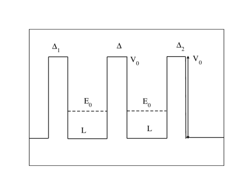
Figure 1: Sequence of potential barriers of finite height and width.

We may compute transmission through the system in a standard way, by matching the wave function and its derivative on either side of each barrier in Fig. 1. Throughout the paper, we will use units with $\hbar^{2}/2m_{e}=1$. Thus, when distances $\Delta$, $\Delta_{1,2}$, and $L$ are measured in nm (the typical scale for semiconductor superlattices), all energies are calculated in units of $38$ meV. In what follows we set $L=2$, $\Delta=0.2$, $V_{0}=1000$, and $E_{0}=V_{0}/2=500$ (so that the energy shift vanishes, see below).

In the limit of weak tunneling between the sites, a sequence of $N$ potential wells behaves as an open $1d$ Anderson model. As shown in Ref. Kaplan , the $1d$ effective Hamiltonian for an energy band centered at $E_{0}$ can be written in the site basis in a way similar to that used in Refs. Zannals ; VZWNMP04 ,

$${\cal H}=\left(\begin{array}[]{ccccc}E_{0}+\delta_{1}-\frac{i}{2}\gamma_{1}&\Omega&0&...&0\\ \Omega&E_{0}&\Omega&...&0\\ 0&\Omega&E_{0}&...&0\\ ...&...&...&...&...\\ 0&0&0&...&E_{0}+\delta_{2}-\frac{i}{2}\gamma_{2}\end{array}\right)\,.$$ (1)

The edge states, $|1\rangle$, localized in the first well on the left, and $|N\rangle$, localized in the last well on the right, acquire finite widths, $\gamma_{1,2}$, and energy shifts, $\delta_{1,2}$, due to the coupling to the environment. By inter-site tunneling, this coupling propagates through the chain.

The effective Hamiltonian ${\cal H}$ correctly reproduces transmission through a sequence of potential barriers if we define the tunneling coupling $\Omega$ as

$$\Omega=\frac{2\alpha^{2}E_{0}}{V_{0}(1+\alpha L/2)}\exp{(-\alpha\Delta)}\,,$$ (2)

where $\alpha=\sqrt{V_{0}-E_{0}}$. Similarly, the widths and energy shifts can be written as

$$\left.\begin{array}[]{lll}\gamma_{1,2}=\frac{8\alpha^{3}E_{0}k}{V_{0}^{2}(1+\alpha L/2)}\exp{(-2\alpha\Delta_{1,2})},\\ \\ \delta_{1,2}=\frac{k^{2}-\alpha^{2}}{4\alpha k}\,\gamma_{1,2}\,,\\ \end{array}\right.$$ (3)

where $k=\sqrt{E_{0}}$. The shifts $\delta_{1,2}$ vanish for $E_{0}=V_{0}/2$; otherwise the sign of $\delta$ is given by the sign of $E_{0}-V_{0}/2$. We will study how the transport properties depend on the system–environment couplings $\gamma_{1,2}$, which are varied by adjusting the external barrier widths $\Delta_{1,2}$ while keeping all other parameters fixed.

With the aid of the effective Hamiltonian, the transmission coefficient $T^{ab}(E)$ from channel $b$ to channel $a$ can be determined,

$$T^{ab}(E)=|Z^{ab}(E)|^{2}\,,$$ (4)

where

$$Z^{ab}(E)=\sum_{i,j=1}^{N}A_{i}^{a}\left(\frac{1}{E-{\cal H}}\right)_{i,j}(A_{j}^{b})^{\ast}$$ (5)

is the transmission amplitude. The channels are labeled by the quantum numbers that characterize the continuum states in the environment, not including the energy. In the $1d$ case we have two channels, $a=1,2$, corresponding to the left and right scattering states, respectively. The factors $A_{i}^{a}$ represent the transition amplitudes from state $|i\rangle$ to channel $a$. In our arrangement, the only non-vanishing transition amplitudes are $A_{1}^{1}=\sqrt{\gamma_{1}}$ and $A_{N}^{2}=\sqrt{\gamma_{2}}$. The complex eigenvalues ${\cal E}_{k}$ of ${\cal H}$ coincide with the poles of $Z(E)$. The spectrum of the complex eigenvalues of the effective Hamiltonian is of great importance for understanding the transport properties of the system.

Using the effective Hamiltonian of Eq. (1), the transmission between left and right leads can be computed as

$$T(E)=\left|\frac{(\sqrt{\gamma_{1}\gamma_{2}}/\Omega)}{\prod_{k=1}^{N}(E-{\cal E}_{k})/\Omega}\right|^{2}\,,$$ (6)

where here and in the following $T(E)\equiv T^{12}(E)$. It was shown in Ref. Kaplan that the exact transmission obtained by matching of the wave functions is in excellent agreement with the effective Hamiltonian approach, Eq. (6), for $\alpha\Delta\gg 1$.

III Transmission Through Nanostructures with Asymmetric Coupling

In this Section we analyze the behavior of the transmission as we increase the coupling to the external environment, keeping the ratio of the two external couplings, $\gamma_{1}=\gamma$ and $\gamma_{2}=\gamma/q$, fixed and equal to $q$, the asymmetry parameter. We treat first the case of no disorder, where the unperturbed states in all sites have the same energy $E_{0}$, and later extend to the disordered case. We will also drop the energy offset $E_{0}$ from the effective Hamiltonian, so that the center of the energy band is always at zero energy, and for simplicity we neglect the energy shifts $\delta_{1,2}$ in the following considerations (which in the potential of Fig. 1 corresponds to $E_{0}=V/2$).

III.1 Ordered Case

Before considering the problem of a general $N$-level system, we first treat the one-well and two-well cases, which give us valuable insight into how transport properties change as we increase the coupling strength to the environment.

We start with the transmission through a single quantum level, namely through a quasistationary state created by two potential barriers. In this case we have only one resonance and the effective Hamiltonian reduces to ${\cal H}=-i\gamma/2-i\gamma/2q$. The resonance height is independent of the coupling $\gamma$, and transmission is never perfect for asymmetric barriers. Indeed, from Eq. (6) we see that maximum transmission is attained at $E=0$ and is given by

$$T(E=0)=\frac{4q}{(q+1)^{2}}\,,$$ (7)

so that $T(E=0)=1$ only for the equal-coupling case of $q=1$.

The situation is different when we consider transmission through two quantum states. This problem has been studied previously, see for instance Refs. VZ03 ; nonthermal and references therein. In fact, many of the results obtained for the two-level case are of more general validity. The effective Hamiltonian for two originally degenerate levels can be written as

$${\cal H}=\left(\begin{array}[]{cc}-\frac{i}{2}\gamma&\Omega\\ \Omega&-\frac{i}{2}\gamma/q\end{array}\right)\,.$$ (8)

From Eq. (6) we can then compute the transmission. In particular, the transmission at $E=0$ is

$$T(E=0)=\left|\frac{(\gamma/\Omega)/\sqrt{q}}{1+(\gamma/\Omega)^{2}/4q}\right|^{2}\,.$$ (9)

At the critical value,

$$\left(\frac{\gamma}{\Omega}\right)_{\rm cr}=2\sqrt{q}\,,$$ (10)

transmission is perfect. This is in contrast with the one-level situation, where transmission is never perfect for $q\neq 1$.

By applying the residue method to Eq. (6), we can also compute the normalized integrated transmission:

$$S=\frac{1}{4\Omega}\int T(E)\,dE=\frac{\pi\gamma/\Omega}{2(q+1)[1+(\gamma/\Omega)^{2}/4q]}\,,$$ (11)

where $4\Omega$ is the width of the energy band. The maximum integrated transmission occurs at the same critical $\gamma$ value given by Eq. (10). The quantitative behavior of $S$ is important in applications, for instance in the design of electron band-pass filters for semiconductor superlattices POT .

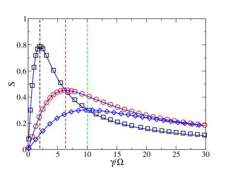
Figure 2: (Color online) Integrated transmission $S$ obtained in the effective Hamiltonian approach for $N=100$ sites and different asymmetry parameters $q$: squares refer to $q=1$, circles to $q=10$, and diamonds to $q=25$. The solid curves represent the result (11) obtained for $N=2$. The vertical dashed lines indicate the critical value of the coupling strength in each case, $\gamma/\Omega=2\sqrt{q}$, where $S$ is predicted to have its maximum, see Eq. (10).

We now analyze transport properties for the general $N$-level system, many of which parallel those of the special one- and two-level cases. Numerically calculating transmission as a function of energy, we find that perfect transmission is attained at all resonance peaks precisely at the critical coupling given by Eq. (10) independently of the value of $N$, see for example the upper right panel of Fig. 6. Moreover, for all $N\geq 2$, the integrated transmission has a maximum at the same value of the coupling. The simple theoretical expression (11), obtained for the integrated transmission in the two-level case, closely reproduces the integrated transmission for any $N\geq 2$, see Fig. 2. The origin of this $N$-independent behavior in the coherent transport regime has been discussed previously in the context of symmetric coupling Kaplan .

Our results agree with the full analytical expression for the transmission amplitude (5) in the general $N$-level case Zannals ,

$$Z(E)=-\,\frac{2\sqrt{\gamma_{1}\gamma_{2}}\,P_{-}(E)}{1+i(\gamma_{1}+\gamma_{2})P_{+}(E)+\gamma_{1}\gamma_{2}[P_{-}^{2}(E)-P_{+}^{2}(E)]},$$ (12)

where

$$P_{\pm}(E)=\,\frac{1}{N+1}\sum_{n=1}^{N}(\pm 1)^{n}\,\frac{1}{E-E_{n}}\,\sin^{2}\left(\frac{\pi n}{N+1}\right),$$ (13)

and the sums are over the unperturbed Bloch wave energies of the closed system,

$$E_{n}=2\Omega\cos\left(\frac{\pi n}{N+1}\right).$$ (14)

This determines the exact transmission probability,

$$T(E)=\,\frac{4\gamma_{1}\gamma_{2}P_{-}^{2}}{\Bigl{[}1+\gamma_{1}\gamma_{2}\Bigl{(}P_{-}^{2}-P_{+}^{2}\Bigr{)}\Bigr{]}^{2}+(\gamma_{1}+\gamma_{2})^{2}P_{+}^{2}}.$$ (15)

Inside the energy band, at any pole $E=E_{n}$ corresponding to a Bloch eigenstate, both sums $P_{\pm}$ diverge with $|P_{+}/P_{-}|\to 1$, and the transmission takes the $N$-independent and $\gamma$-independent value given by Eq. (7),

$$T(E=E_{n})=T_{1}\equiv\frac{4q}{(q+1)^{2}}\,,$$ (16)

obtained above for $E=0$ in the special case $N=1$. Outside the band, for $|E|>2\Omega$, the sum $P_{+}$ converges at large $N$ to the $N$-independent value

$$P_{+}(\epsilon)\approx\frac{z_{\mp}}{2\Omega}$$ (17)

(see Appendix), whereas the sum $P_{-}$ is exponentially small at large $N$,

$$P_{-}(\epsilon)\approx\mp\frac{\sqrt{\epsilon^{2}-1}}{\Omega z_{\pm}^{N+1}}\,,$$ (18)

where $\epsilon=E/2\Omega$ and $z_{\pm}=\epsilon\pm\sqrt{\epsilon^{2}-1}$. The fast decay of $P_{-}$ results in exponentially weak transmission. In Eqs. (17) and (18), the upper and lower signs should be chosen for $\epsilon>1$ and $\epsilon<-1$, respectively. For energies $E$ inside the band, the sums in Eq. (13) take a simple form, see Appendix:

$$P_{\pm}(\epsilon)\approx\frac{1}{2\Omega}\begin{cases}\frac{\sin(N\beta)}{\sin[(N+1)\beta]}\\ -\frac{\sin(\beta)}{\sin[(N+1)\beta]}\end{cases}\,,$$ (19)

where $\beta=\cos^{-1}(\epsilon)$.

A convenient simplification does occur for energies near the middle of the band, $|E|\ll\Omega$, where for large $N$ the sums $P_{\pm}$ are dominated by terms associated with $n\approx N/2$, while distant contributions from the left and right sides of the Bloch spectrum cancel. Near the center of the band, $E_{n}$ may be replaced by a picket fence spectrum with spacing $D=2\pi\Omega/N$, while the last factor in Eq. (13) reduces to unity. Defining $r$ by $E=E_{n_{0}}+rD$, we then have the $N-$independent result

$$P_{\pm}(E)\approx\frac{1}{2\Omega}\begin{cases}\cot(\pi r)\\ (\pm 1)^{n_{0}}\csc(\pi r)\end{cases}\,,$$ (20)

and therefore

$$T(E)\approx\frac{16\gamma_{1}\gamma_{2}}{(4\Omega+\gamma_{1}\gamma_{2}/\Omega)^{2}\sin^{2}(\pi r)+4(\gamma_{1}+\gamma_{2})^{2}\cos^{2}(\pi r)}\,.$$ (21)

At energies in the Bloch spectrum ($r=0$), Eq. (21) reduces, as it must, to the exact expression (16), while midway between any two neighboring poles ($r=1/2$) the transmission becomes

$$T(E=E_{n}+D/2)\approx T_{2}\equiv\left|\frac{(\gamma/\Omega)/\sqrt{q}}{1+(\gamma/\Omega)^{2}/4q}\right|^{2}\,,$$ (22)

which agrees with the transmission at $E=0$ obtained above in the special case of $N=2$ wells, Eq. (9). At these energy midpoints, perfect transmission occurs at the critical value of the coupling given by Eq. (10), just as it does in the special case $N=2$. Averaging Eq. (21) over an energy window containing multiple resonances, $\Omega/N\ll\Delta E\ll\Omega$, we obtain the energy-averaged transmission near the middle of the band,

$$\overline{T}=\int_{0}^{1}T(E)\,dr\approx\frac{8\gamma/\Omega}{(q+1)(4+(\gamma/\Omega)^{2}/q)}\,,$$ (23)

that reaches its maximum, $T_{\rm avg}^{{\rm max}}=2\sqrt{q}/(1+q)$, again at the critical value of the coupling $\gamma/\Omega$ given by Eq. (10).

The critical value associated with the maximum transmission in Fig. 2 is also consistent with the results of Ref. PB . There, the authors found that given a sequence of potential barriers of width $\Delta$, adding two external barriers satisfying $\Delta_{L}+\Delta_{R}=\Delta$ produces an increase in transmission while leaving the resonance energies unchanged. From Eqs. (2) and (3), we can see that the maximum transmission condition (10) obtained from the tight-binding model coincides with the condition $\Delta_{L}+\Delta_{R}=\Delta$ for the case of $E_{0}=V_{0}/2$, in which case the energy shift is zero.

III.2 Disordered Case

In this subsection we analyze the effect of disordered on-site energies. The survival of the super-radiant restructuring in the disordered chain was established in Ref. VZWNMP04 . In Ref. Kaplan we showed that the effective Hamiltonian, Eq. (1), correctly describes the sequence of potential barriers in the presence of disorder (e.g., variable well width), when the disorder is sufficiently weak. We consider random variations of the diagonal energies, $E_{0}+\delta E_{0}$, where $\delta E_{0}$ is uniformly distributed in the interval $[-W/2,+W/2]$, and $W$ is the disorder parameter. In Ref. Kaplan it was shown that for $\alpha\Delta\gg 1$, a random variation of $\delta E_{0}$ in the interval $[-W/2,+W/2]$ corresponds to a random variation of the well width $\delta L$ in $[-WL/4E_{0},+WL/4E_{0}]$.

The effective non-Hermitian Hamiltonian with diagonal disorder is equivalent to a $1d$ open Anderson tight-binding model Anderson ; Lee . The eigenstates of the Anderson model are exponentially localized on the system sites, with the tails given by $\exp(-x/L_{\rm loc})$. Here the localization length $L_{\rm loc}$ depends on the disorder strength Felix , and $x$ is distance in the direction of transmission, measured in units of the well size. For $L_{\rm loc}\ll N$, the transmission decays exponentially with $N$; this is the localized regime.

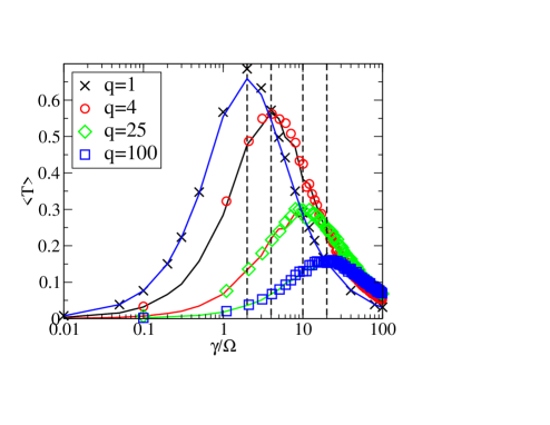
Figure 3: (Color online) Average transmission near $E=0$ as a function of coupling strength $\gamma/\Omega$ for a disordered $1d$ chain of $N=100$ wells, for different values of the asymmetry parameter $q$. The disorder strength is $W/\Omega=0.5$. Each value of transmission corresponds to the average over an energy window $-0.1<E<0.1$, and ensemble average over $100$ realizations of the disorder. The curves are obtained from the effective Hamiltonian ${\cal H}$ (open Anderson model), whereas symbols are computed for the sequence of potential barriers. Vertical dashed lines indicate the critical values of the coupling (10) for the ordered case.

Let us first consider the case when the mean level spacing $D$ (at the center of the energy band) is not strongly modified by the disorder. In the ordered case, $D\approx 2\pi\Omega/N$ for $E=0$, while for strong disorder the band width is $W$ and we have $D\approx W/N$. Thus, we expect that for $W<2\pi\Omega$ the mean level spacing is not strongly influenced by the disorder. This regime is shown in Fig. 3, where we plot the average transmission as a function of the coupling strength $\gamma/\Omega$ for $N=100$ and $W/\Omega=0.5$. As indicated by the vertical dashed lines, the maximum transmission is reached at the same critical values of $\gamma/\Omega$ obtained previously in the absence of disorder, Eq. (10). At this critical value, each transmission curve intersects the transmission curve for the symmetric case $q=1$. Indeed, at the critical coupling, the tunneling probabilities from the left and right are equal, implying that for this value the asymmetric system behaves as a system with symmetric coupling, see Sec. V.

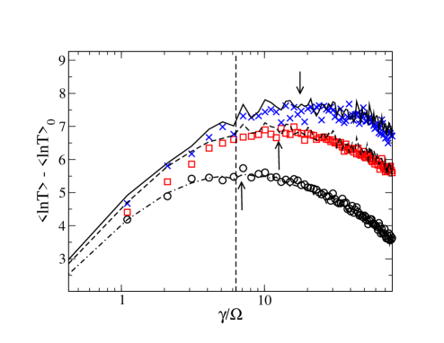
Figure 4: (Color online) Average of the logarithm of transmission at $E=0$ as a function of the coupling $\gamma/\Omega$ for the $1d$ case, with $N=100$ sites, and asymmetry parameter $q=10$. In our units, the tunneling coupling is $\Omega=1$, and the three data sets correspond to different disorder strengths $W$. $\langle\ln T\rangle_{0}$ represents the value of the transmission at $\gamma/\Omega=0.01$, which is the lowest value of $\gamma/\Omega$ computed. For the sake of clarity, we plot $\langle\ln T\rangle-\langle\ln T\rangle_{0}$ so that all data start from the same point. In each case, symbols refer to the results obtained from the effective Hamiltonian ${\cal H}$: circles for $W=4$, squares for $W=10$, and crosses for $W=15$, while the curves refer to a sequence of potential barriers: dot-dashed for $W=4$, dashed for $W=10$, and solid for $W=15$. Averaging is performed over $1000$ realizations of the disorder. The dashed vertical line indicates the critical value of the coupling, Eq. (10), at which transmission is maximized for low disorder. The arrows indicate $\gamma/\Omega=1.2ND/\Omega$, where $D$ is the mean level spacing at the center of the energy band and the factor $1.2$ is obtained from fitting.

The situation is different for strong disorder, $W>2\pi\Omega$. The critical value for maximized transmission now depends on the disorder strength. For strong disorder we enter the localized transport regime studied in Ref. Beenakker , where transmission is log-normally distributed, so that it is more convenient to consider the average of $\ln T$ rather than the average of $T$. Numerically we find that the value at which transmission is maximized is proportional to the mean level spacing $D$ at the center of the energy band: $\gamma\propto ND$, see the arrows that indicate $\gamma=1.2ND$ for each curve in Fig. 4, where $q=10$. Since $D\approx W/N$ when disorder is strong, the critical value of the coupling is in this case proportional to the disorder strength.

Additionally, we note the close agreement between symbols and solid curves in Figs. 3 and 4, demonstrating good correspondence between the exact barrier problem, Fig. 1, and the energy-independent effective Hamiltonian of Eq. (1). This correspondence persists for weak and strong coupling to the environment, in highly symmetric and highly asymmetric situations, and also for both weak and strong disorder.

IV Double Super-Radiant Transition and Structure of Resonances

In Ref. Kaplan we showed that maximum transmission is reached at the super-radiant transition in the symmetric coupling case. The transition is signaled by a segregation of resonance decay widths, i.e., of the imaginary parts of the eigenvalues of the effective Hamiltonian, into two groups, super-radiant (short-lived) and trapped (long-lived) SZNPA89 ; Zannals ; Kaplan ; izr94 . The number of super-radiant states is equal to the number of channels coupling the system to the environment [two for Fig. 1 and for the effective Hamiltonian of Eq. (1)]. In order to identify the super-radiance transition we compute the average of the non-super-radiant widths, i.e. of the smallest $N-2$ decay widths of the effective Hamiltonian. In Fig. 5, we plot this average value as a function of the coupling $\gamma/\Omega$ for two asymmetry values, $q=4$ and $q=10$. In each case the average width shows two maxima as $\gamma/\Omega$ is varied. At each maximum, one of the widths segregates from the others. Thus, in the presence of asymmetry, we have two super-radiant transitions associated with two critical values of the coupling. According to the resonance overlap condition, $\gamma_{1,2}/\Omega=2$ Kaplan , the two transitions are predicted to occur at the values

$$(\gamma/\Omega)_{\rm SR1}=2,\hskip 14.22636pt\hskip 5.69046pt(\gamma/\Omega)_{\rm SR2}=2q,$$ (24)

indicated by the vertical dashed lines in Fig. 5, in very good agreement with the numerical results for different values of the asymmetry.

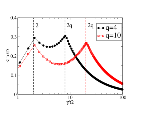
Figure 5: (Color online) Average width (computed over the smallest $N-2$ widths) in units of the mean level spacing at the center of the energy band. The average width is calculated as a function of $\gamma/\Omega$ for $N=100$ and two values of the asymmetry parameter $q$. Dashed vertical lines indicate the locations of the two super-radiant transitions, as given by Eq. (24).

Comparing Eqs. (10) and (24), we observe that, in the presence of asymmetry, the point of maximum transmission is always in between the two super-radiant transitions. The transmission maximum occurs approximately at the minimum of the average decay width, while the super-radiant transitions occur at the two maxima of the average decay width. This can be compared to the case of symmetric barriers, where the maximal transmission precisely coincides with the (single) super-radiant transition Kaplan , in agreement with Eq. (24) for $q=1$.

Since the super-radiant states are very broad, the number of observed resonances changes after each transition. As we increase the coupling, the number of resonances changes from $N$ at weak coupling to $N-1$ after the first transition, and finally to $N-2$ for strong coupling. This change in the resonance structure can have important consequences for experimental current-voltage curves, for example in semiconductor superlattices TsuEsaki . For symmetric coupling, the number of resonances changes directly from $N$ to $N-2$ at the (single) super-radiant transition Kaplan .

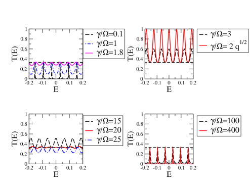
Figure 6: (Color online) Transmission for $N=100$ and asymmetry parameter $q=10$ calculated as a function of energy in a small interval around the center of the energy band. Ten different values of the coupling $\gamma/\Omega$ are shown for the case of no disorder, $W=0$. The horizontal dashed line, Eq. (16), is the analytically obtained transmission at the location of the poles, which is also the maximum transmission for $N=1$, Eq. (7).

An important consequence of the two super-radiant transitions can be seen in the structure of resonances near the center of the energy band. In Fig. 6 we consider a $1d$ chain with $N=100$, $q=10$, and no disorder ($W=0$), and calculate transmission as a function of energy for different values of the coupling $\gamma/\Omega$. In each panel in Fig. 6, the dashed horizontal line indicates the transmission at energy values belonging to the Bloch spectrum, Eq. (16), which is also the maximal transmission attainable for transport through one level only, as given by Eq. (7).

In the upper left panel of Fig. 6, the resonance structure is shown for several cases of weak coupling, $\gamma/\Omega<2$, i.e. below the first super-radiant transition. The maximum resonance height is here independent of $\gamma/\Omega$, and equal to the single-level resonance height. Only the widths grow as $\gamma/\Omega$ is increased in this regime. In the upper right panel, we consider $2<\gamma/\Omega<2q$, the intermediate regime between the two super-radiant transitions. Perfect transmission is reached for all resonances precisely at the geometric mean of the two transitions, at $\gamma/\Omega=2\sqrt{q}$. In this regime, it is the minimum transmission that is independent of $\gamma/\Omega$ and equal to the single-resonance transmission height, Eq. (7). In the lower left panel the region around the second super-radiant transition is shown. As $\gamma/\Omega$ crosses the value $\gamma/\Omega=2q$, the minimum transmission drops below the one-level transmission value. Finally, in the lower right panel, we show the regime of large coupling, $\gamma/\Omega>2q$. Here it is again the maximum transmission that is independent of $\gamma/\Omega$ and given by Eq. (7), just as in the weak coupling regime, but the resonance widths now shrink with increasing $\gamma/\Omega$. The behavior shown in Fig. 6 indicates that, at least for large $N$, a qualitative change in the resonance structure near the center of the energy band occurs at each of the two super-radiant transitions.

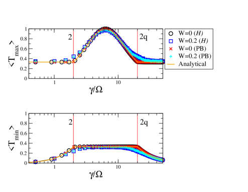
Figure 7: (Color online) The case of $N=100$ sites with $q=10$ is considered. Upper panel: the resonance height (transmission maximum) averaged over the center of the band ($-0.1<E<0.1$), as a function of $\gamma/\Omega$. Lower panel: the transmission minimum averaged over the same energy window. The two vertical lines indicate the positions of the two super-radiant transitions. The solid curve shows the predictions of Eqs. (25) and (26). A clear change in the transport properties is seen at each of the two transitions. The effect persists in the presence of disorder ($W/\Omega=0.2$). In each panel, the results obtained from the effective Hamiltonian (${\cal H}$) are compared with those obtained from the sequence of potential barriers (PB).

To better study this change in the resonance structure, we now compute $\langle T_{\rm max}\rangle$, the average of the transmission maxima, and $\langle T_{\rm min}\rangle$, the average of the transmission minima, as functions of the coupling strength. In each case, the averaging is performed over a window near the center of the energy band, $-0.1<E<0.1$. The upper panel of Fig. 7 shows that $\langle T_{\rm max}\rangle$ is constant to the left of the first super-radiant transition and to the right of the second transition (shown as vertical lines). The constant value coincides with that for the one-level maximal transmission, Eq. (7), as shown by the horizontal line. Between the two transitions, $\langle T_{\rm max}\rangle$ reaches a maximum value at $\gamma/\Omega=2\sqrt{q}$. In the lower panel of Fig. 7, we show the behavior of $\langle T_{\rm min}\rangle$ as a function of $\gamma/\Omega$. This average rises to reach the one-level transmission value at the first transition, stays constant up to the second transition, and then decreases.

For the ordered case we then find numerically the simple results:

$$\langle T_{\rm max}\rangle=\left\{\begin{array}[]{cc}T_{2}&{\rm for}\hskip 5.69046pt2\leq\gamma/\Omega\leq 2q\\ T_{1}&{\rm otherwise}\end{array}\right.\,,$$ (25)

and

$$\langle T_{\rm min}\rangle=\left\{\begin{array}[]{cc}T_{1}&{\rm for}\hskip 5.69046pt2\leq\gamma/\Omega\leq 2q\\ T_{2}&{\rm otherwise}\end{array}\right.\,,$$ (26)

which agree well with the analysis in Sec. III.1. Here $T_{1}$ is the transmission at resonant energies in the Bloch spectrum, Eq. (16), that coincides with the one-level maximal transmission value, Eq. (7). Similarly, $T_{2}$ is the transmission value at midway points between these energies, Eq. (22), that coincides with $T(E=0)$ for the two-level case, Eq. (9). These formulas, represented by the solid lines in Fig. 7, are in good agreement with the numerical calculation.

It is also interesting to point out that from the analytical expressions, Eqs. (22) and (16), we have that $T_{2}\geq T_{1}$ for $2\leq\gamma/\Omega\leq 2q$, so that we regain the thresholds for the two super-radiant transitions.

In the same Figure, we also illustrate the effect of adding disorder. For weak disorder, the behavior is similar to the ordered case, while for strong disorder the effect of the two super-radiant transitions is smoothed out. In Fig. 7 the results obtained from the effective Hamiltonian (circles and squares) are compared with the results from the sequence of potential barriers (crosses and pluses). Again, the agreement is excellent, both with and without disorder.

V Comparison with Random Matrix Theory

It is interesting to compare our results on the $1d$ Anderson model with standard results obtained in the framework of the random matrix theory of transport. In Ref. Weiden , the dependence of the conductance on the degree of opening was analyzed for a quasi-$1d$ system with symmetric coupling to the leads, while the case of asymmetric coupling was later addressed in Ref. Beenakker , with different tunneling probabilities for the right and left ends. The tunneling probability used in Ref. Beenakker corresponds to the “elastic scattering” probability $\tau$ defined in Ref. puebla , where the case of symmetric coupling and varying degree of internal disorder was considered. This probability for channel $a$ is defined as $\tau^{a}=1-|\langle S^{aa}\rangle|^{2}$, where $S$ is the scattering matrix, $S^{ab}=\delta^{ab}-iZ^{ab}$, and $Z^{ab}$ is given by Eq. (5). Again, we take $a=1,2$ to be the channels corresponding to the left and right scattering states, respectively. From Ref. puebla we know that in the random matrix framework and at the center of the energy spectrum

$$\tau_{1,2}=\frac{4\kappa_{1,2}}{(1+\kappa_{1,2})^{2}}\,,$$ (27)

where $\kappa_{1,2}$ is the effective coupling to channel $1$ and $2$, respectively. In the special case when the internal system is described by a GOE random matrix,

$$\kappa_{1,2}=\frac{\pi\gamma_{1,2}}{2ND}\,,$$ (28)

where $D$ is the mean level spacing at the center of the spectrum and $N$ is the dimension of the internal system. As before, in the presence of asymmetry, $\gamma_{1}=\gamma$ and $\gamma_{2}=\gamma/q$.

For asymmetric coupling, maximum transmission is achieved when $\tau_{1}=\tau_{2}$ Beenakker . At this special point, the system with asymmetric coupling behaves as a system with symmetric coupling. This happens in the trivial case $\kappa_{1}=\kappa_{2}$ (where the coupling is symmetric to begin with) or for $\kappa_{1}=1/\kappa_{2}$. Since in the $1d$ case we have $ND\approx 2\pi\Omega$ at the center of the energy band and for moderate disorder, we find from Eqs. (27) and (28) that the maximum transmission should be achieved when $\gamma/\Omega=4\sqrt{q}$, which is off by a factor of two from the value given by Eq. (10).

In order to understand the origin of this difference, we rederive below Eqs. (27) and (28) in a slightly different way, following the approach of Refs. puebla . The scattering matrix averaged over the ensemble of random realizations is given by

$$\langle S\rangle=\frac{1-i\langle K\rangle}{1+i\langle K\rangle}$$ (29)

to leading order in $1/N$ SZNPA89 ; puebla . Here $S^{ab}$ and $K^{ab}$ are matrices in the channel space, with the explicit expression for $K^{ab}$ given below in Eq. (30). Eq. (29) is valid, under the assumption that the internal system can be described by random matrix theory, when the elements of $K$-matrices in the numerator and the denominator of Eq. (29) are effectively uncorrelated since their correlations lead only to corrections no larger than $\sim 1/N$. In the $1d$ Anderson model, the above assumption breaks down both in the limit of very weak disorder, where the internal system approaches integrability, and also for extremely strong disorder, where we enter the localized regime.

The $K$-matrix in channel space can be written as

$$K^{ab}(E)=\frac{1}{2}\,\sum_{n}\frac{B^{a}_{n}B^{b\ast}_{n}}{E-E_{n}},$$ (30)

where real energies $E_{n}$ are the eigenvalues of the closed system. In our case of two channels, $B^{1}_{n}=\sqrt{\gamma_{1}}\langle 1|\psi_{n}\rangle$ and $B^{2}_{n}=\sqrt{\gamma_{2}}\langle N|\psi_{n}\rangle$ are the transition amplitudes for the eigenstate $|\psi_{n}\rangle$ to the left and right leads, respectively. The sum in Eq. (30) contains the eigenvalues of the resolvent $1/(E-H)$ of the closed system. For energy $E$ inside the spectrum of $H$ we should understand it as a limiting value, $E\rightarrow E+i0$. Using the identity

$$\frac{1}{E-E_{n}+i0}={\rm P.v.}\,\frac{1}{E-E_{n}}-i\pi\delta(E-E_{n})\,,$$ (31)

and replacing the summation with the integral, we can compute the average $K$-matrix. The principal value part is a smooth function of energy that vanishes in the middle of the spectrum; as a result, in this vicinity

$$\langle K^{11}\rangle=-\frac{i\pi}{2}\langle|B^{1}_{E_{n}=0}|^{2}\rangle\rho(E=0)=-i\kappa_{1}\,,$$ (32)

where $\rho(E=0)=1/D$ is the density of states at the center of the spectrum. Thus we have

$$\kappa_{1,2}=\frac{\pi|B^{1,2}_{E_{n}=0}|^{2}}{2D}\,,$$ (33)

which we can use in Eq. (27). In particular, if the eigenstate components are assumed to obey random matrix statistics, we have $|B^{1,2}_{E_{n}=0}|^{2}=\gamma_{1,2}/N$, and we recover Eq. (28).

We analyze the statistics of the $1d$ Anderson model eigenstates in Fig. 8, where we plot the ensemble-averaged value of $|\langle 1|\psi_{n}\rangle|^{2}$ (the probability overlap of the eigenstate $|\psi_{n}\rangle$ with a state localized at the left edge of the chain, that for a weakly open system would determine the width distribution for intrinsic states) as a function of $E_{n}$ for different strengths of disorder. Evidently, the components of the eigenstates do not follow random matrix theory for moderate disorder. Near the center of the energy band we have $\langle|\langle 1|\psi_{n}\rangle|^{2}\rangle\approx 2/N$ for $W/\Omega=0.5$ and $W/\Omega=1$. Then from Eq. (33) we obtain

$$\kappa_{1,2}=\frac{\gamma_{1,2}}{2\Omega}\,,$$ (34)

and $\gamma_{\rm cr}/\Omega\approx 2\sqrt{q}$, in agreement with our findings in the previous sections. The values of $\gamma/\Omega$ at which we have perfect tunneling probability, $\gamma/\Omega=2$, where $\tau_{1}=1$, and $\gamma/\Omega=2q$, where $\tau_{2}=1$, coincide precisely with the values of $\gamma$ at which the two super-radiant transitions occur, see the discussion in Sec. IV. The fact that perfect tunneling probability $\tau$ is reached at the super-radiant transition has been pointed out in Refs. puebla .

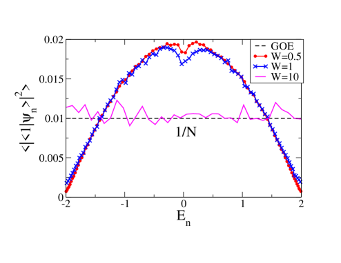
Figure 8: (Color online) Overlap probability of an eigenstate at energy $E_{n}$ with the edge $|1\rangle$ of the chain in the $1d$ Anderson model for $N=100$. The result is averaged over $10^{4}$ random realizations and plotted versus energy for different disorder values $W$ (in units $\Omega=1$). The theoretical value for a GOE random matrix is indicated by a dashed horizontal line.

From Fig. 8 we see that for large values of $W$ we have $\langle|\langle 1|\psi_{n}\rangle|^{2}\rangle\approx 1/N$, but in this regime the eigenstates are strongly localized and we no longer expect Eq. (29) to be valid. The dip in the value of $\langle|\langle 1|\psi_{n}\rangle|^{2}\rangle$ at the center of the energy band shown in Fig. 8 is consistent with the analysis of Ref. Felix , where it was pointed out that the localization length is shorter at the center of the energy band than for surrounding energies.

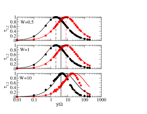
Figure 9: (Color online) Left and right tunneling probabilities $\tau_{1,2}$ are plotted vs $\gamma/\Omega$ for three different disorder strengths $W$, in units $\Omega=1$, for the system size $N=100$ and asymmetry parameter $q=4$. The numerical results (symbols) are obtained by averaging over $10^{3}$ disorder realizations and over an energy interval $-0.1<E<0.1$ around the center of the spectrum. These are compared with the theoretical results (solid curves) obtained from Eqs. (34) and (27). The critical value of $\gamma/\Omega$, Eq. (10), is indicated by a vertical solid line in each panel. In the upper and middle panels, the values at which perfect transmission is reached, $\gamma/\Omega=2$ and $\gamma/\Omega=2q$, are shown as vertical dot-dashed lines.

In Fig. 9 we compare our numerical results for the tunneling probability $\tau$ with Eqs. (27) and (34), showing reasonable agreement for moderate disorder $W/\Omega=0.5$, $1$. For $W/\Omega=10$, clear deviations from the analytical expressions are visible, due to the fact that the assumptions of random matrix theory break down at very strong disorder.

These results show that a blind application of random matrix results would lead to incorrect conclusions for the $1d$ Anderson model. Our empirical expression for the tunneling probability works well for moderate disorder. In this regime, we regain the critical value of the coupling strength (10) for which maximum transmission is achieved.

VI Multi-Dimensional Case

In this Section, we discuss the higher-dimensional cases. Only selected results will be shown, sufficient to demonstrate that the general behavior of the maximum transmission found in $1d$ systems can be extended to higher dimensions.

The open model in dimensions greater than one consists of an array of sites with associated energy levels. Neighboring sites are coupled to each other by the tunneling coupling $\Omega$, as in the $1d$ case. In higher dimensions, we have many ways to couple the system to external leads. In the $2d$ case, where the number of sites in a rectangular array is $N=M\times L$, we couple each of the $M$ sites on the left side to a separate left lead and each of $M$ sites on the right side to a separate right lead, see Fig. 10. The coupling amplitude for each of the $M$ left leads is $\gamma_{1}=\gamma$, while the coupling amplitude to each of the $M$ right leads is $\gamma_{2}=\gamma/q$. Similarly, in the $3d$ case, with $N=M\times M\times L$ sites, each site on an $M\times M$ face is coupled to a lead. In this geometry, each lead represents a channel. Such an open model can describe a variety of physical systems, such as an array of quantum dots, or a particle trapped in a lattice potential.

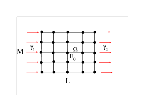
Figure 10: Two-dimensional open model used in this paper, with $N=M\times L$ sites coupled to $M$ incoming left channels and $M$ outgoing right channels. Specifically, in this Figure we show $M\times L=5\times 5$ sites coupled to $2M=10$ channels. At each site there is a bound state with energy $E_{0}$ coupled to its nearest-neighbor sites through a tunneling amplitude $\Omega$.

The diagonal part of the effective Hamiltonian for this system can be written as ${\cal H}_{ii}=E_{0}+\delta E_{0}$ for sites $i$ that are not coupled to leads, and ${\cal H}_{ii}=E_{0}+\delta E_{0}+\delta_{1,2}-(i/2)\gamma_{1,2}$ for sites coupled to the left or right leads, respectively. As in the $1d$ case, we set the center $E_{0}$ of the energy band to zero; $\delta E_{0}$ is a random variable uniformly distributed in $[-W/2,+W/2]$, and $W$ is a disorder parameter. As before, $\delta_{1,2}$ and $\gamma_{1,2}$ represent the energy shift and decay probability (inverse lifetime), respectively, induced by the coupling to the left and right leads. In the following we again neglect the energy shift, so that $\delta_{1,2}=0$. Finally, for the off-diagonal matrix elements, $i\neq j$, we have ${\cal H}_{ij}={\cal H}_{ji}=\Omega$ if the sites $i$ and $j$ are neighboring and ${\cal H}_{ij}=0$ otherwise.

Depending on the degree of disorder, different transport regimes are possible in the multidimensional case. The ballistic regime is defined by the condition $L<l$, where $L$ is the system length and $l$ is the mean free path. The diffusive regime is determined by the condition $l<L<L_{\rm loc}$, where as before $L_{\rm loc}$ is the localization length. Finally, for $L_{\rm loc}<L$, we are in the localized regime. The mean free path and the localization length both depend strongly on the energy interval under consideration and on the disorder strength, see the discussion in Refs. sheng ; 2D .

In our multidimensional arrangement, a double super-radiant transition again occurs as in $1d$, which we do not discuss in detail here. In this Section we will focus on the dependence of the maximum conductance on the coupling strength to the leads. The dimensionless conductance $G$, which is proportional to the total transmission, can be computed using the Landauer formula Beenakker ; epl ,

$$G(E)=\sum_{a=1}^{M}\sum_{b=M+1}^{2M}|Z^{ab}(E)|^{2}\,.$$ (35)

Here $Z^{ab}(E)$ is the transmission amplitude between channels $a$ and $b$, see Eq. (5), that can be computed from the effective Hamiltonian.

We will not consider here the case of a small perturbation to an integrable Hamiltonian, which displays very system-specific behavior, and start by analyzing the case of moderate disorder. In Fig. 11, we illustrate the behavior of the average conductance in the diffusive regime for a quasi-$1d$ lattice of $M\times L=10\times 100$ sites with $W/\Omega=\sqrt{3/4}$, upper panel, and for a square $2d$ lattice of $30\times 30$ sites with $W/\Omega=2$, lower panel. In both cases, the maximum conductance is obtained at the critical value of the coupling given by Eq. (10). In the upper panel, we compare our numerical results with analytical expressions obtained in the context of random matrix theory Beenakker . The numerically computed left and right transmission coefficients as functions of $\gamma/\Omega$ were used to evaluate the analytical expression for the average conductance given in Ref. Beenakker . In the upper panel of Fig. 11, the numerical results (symbols) are in good agreement with the analytical results (solid curves) for a quasi-$1d$ system in the diffusive regime. To the best of our knowledge, there are no known analytical results for the $2d$ case in the diffusive regime with asymmetric coupling (lower panel).

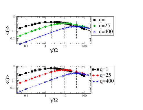
Figure 11: (Color online) The average dimensionless conductance as a function of the coupling strength $\gamma/\Omega$. In the upper panel we consider the quasi-$1d$ case of $10\times 100$ sites in the diffusive regime, with disorder $W/\Omega=\sqrt{3/4}$, so that $L/l\approx 3$. The analytical results of random matrix theory  Beenakker (solid lines) are compared with our numerical results (symbols). In each case, an overall multiplicative factor in the analytical expression Beenakker has been obtained by fitting to the numerical data. In the lower panel, we consider the $2d$ case with $30\times 30$ sites and $W/\Omega=2$, so that $L/l\approx 4$. Here symbols refer to our numerical results and the dashed lines simply connect the symbols (random matrix results are not available for asymmetric $2d$ systems in the diffusive regime). Vertical dashed lines indicate the critical values $\gamma/\Omega=2\sqrt{q}$, where the maximum conductance is expected for each asymmetry value $q$. All numerical results are obtained by averaging over $200$ realizations of disorder and over $100$ different energies in the interval $-0.1<E<0.1$ around the center of the energy band.

At the critical value of $\gamma/\Omega$ given by Eq. (10), each conductance curve for the asymmetric case intersects the conductance curve for the symmetric case ($q=1$). This is similar to what we have observed in the $1d$ case (see Fig. 3), and is also consistent with the results obtained in the context of random matrix theory. As discussed in Sec. V, the maximum conductance is achieved when $\tau_{1}=\tau_{2}$. In this case a system with asymmetric coupling behaves as a system with symmetric coupling.

In the regime of very strong disorder, the critical value at which we have maximum conductance becomes dependent on the mean level spacing, $D$. Similarly to the $1d$ case we have

$$\gamma_{\rm cr}\propto ND\,.$$ (36)

Since in this regime $D\approx W/N$, we find that the critical coupling for the maximum conductance is proportional to the disorder strength $W$, see Fig. 12.

For strong disorder, we enter the localized transport regime, where the transmission is log-normally distributed Beenakker , so that, similarly to Fig. 4, it is more convenient to consider the average of $\ln G$ rather than the average of $G$. In Fig. 12 we plot the average logarithm of the conductance as a function of $\gamma/\Omega$ in $2d$, upper panel, and in $3d$, lower panel. As indicated by the arrows, the critical value of $\gamma/\Omega$ at which the conductance is maximized is in both cases proportional to the mean level spacing, which in turn is proportional (for strong disorder) to the disorder strength. For moderate disorder in either $2d$ or $3d$, see e.g. $W=2$ in the upper panel and $W=5$ in the lower panel, the critical value of $\gamma/\Omega$ for which we have the maximum conductance is again given by Eq. (10). A detailed comparison between random matrix results and the Anderson model will be presented elsewhere.

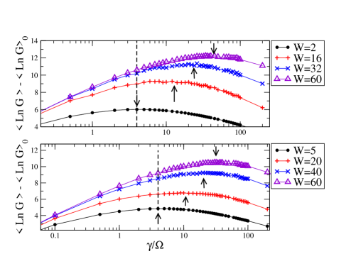
Figure 12: (Color online) Average logarithm of the conductance as a function of the coupling strength $\gamma/\Omega$ for the multidimensional case, with $\Omega=1$, asymmetry parameter $q=4$, and different disorder strengths $W$. For the sake of clarity, we plot $\langle\ln G\rangle-\langle\ln G\rangle_{0}$ so that all data start from the same point, where $\langle\ln G\rangle_{0}$ is defined as in Fig. 4. In the upper panel, we show the $2d$ case with $20\times 20$ sites, while in the lower panel we show the $3d$ case, with $8\times 8\times 8$ sites. The dashed vertical line shows the critical value of the coupling, Eq. (10), at which we have maximum conductance for moderate disorder. The arrows indicate $\gamma/\Omega=0.76ND/\Omega$ for the $2d$ case, upper panel, and $0.56ND/\Omega$ for the $3d$ case, lower panel. The numerical factors $0.76$ and $0.56$ have been found from fitting. All data have been obtained by averaging the conductance over $10^{4}$ ensemble realizations at the center of the energy band, $E=0$.

VII Conclusion

We have analyzed coherent quantum transport through a finite sequence of potential barriers with asymmetric coupling to the external environment. As the coupling to the environment is varied, transport properties are greatly affected. In a previous paper Kaplan , the super-radiant transition that occurs in this paradigmatic model, at a critical value of the coupling, was studied for the case of symmetric coupling to environment. Here, with the aid of the effective non-Hermitian Hamiltonian, we show that for asymmetric coupling a double super-radiant transition occurs, as compared with a single transition in the symmetric case.

The super-radiant transitions have important consequences for the observable resonance structure. In particular, the number of resonances decreases by one after each transition. Focusing on the behavior of transmission near the energy band center, see Fig. 7, we demonstrate that a sharp change in the structure of the resonance occurs in correspondence with the two super-radiant transitions. This change can be characterized by the behavior of the transmission maxima and minima, which we describe analytically as functions of the coupling to the environment and of the asymmetry of this coupling. As far as we know, these features of the structure of resonances as a function of the coupling strength to the leads have not previously been reported in the literature.

Maximum transmission through the system is reached at a coupling $\gamma/\Omega=2\sqrt{q}$, where $q$ is the asymmetry parameter. This coupling is equal to the geometric mean of the coupling strengths associated with the two transitions. We show that this result does not follow from random matrix theory, as usually assumed in statistical theories of quantum transport. Moreover, for very strong disorder we show that the coupling at which transmission is maximized is proportional to the disorder strength. We also find that the latter results remain valid in higher dimensions. Specifically, we analyze the average conductance as a function of the degree of opening, of the asymmetry, and of the strength of disorder in the multidimensional cases: quasi-$1d$, $2d$, and $3d$. In the quasi-$1d$ case, we compare our results with analytical expressions obtained in the context of random matrix theory. We demonstrate the validity of our results in $2d$ and $3d$, in both diffusive and localized transport regimes, where, to the best of our knowledge, no analytical results as a function of the asymmetry of the opening are available in the literature.

The results presented here are based on an approach originally formulated in the framework of nuclear reaction theory. Now we understand that they reflect general properties of quantum signal transmission. Therefore they might be of relevance for numerous applications. The sequence of potential barriers is a paradigmatic model for coherent quantum transport. A better understanding of this transport regime is essential for the development of information technology using different nanoscale systems with complex geometry, including quantum dots, photonic crystals, and molecular wires.

Appendix A Analytical Derivation of the Transmission in the Ordered Case

To derive closed analytical expressions for the sums (13), it is convenient to double them, making the phase $\varphi_{n}=n\pi/(N+1)$ run over the whole circle. Then

$$P_{\pm}(\epsilon)=\frac{1}{2\Omega}\frac{1}{2N+2}\sum_{n=0}^{2N+1}(\pm 1)^{n}\frac{\sin^{2}(\varphi_{n})}{\epsilon-\cos(\varphi_{n})}\,,$$ (37)

where $\epsilon=E/2\Omega$. Now the sum over $n$ spans all the roots $z_{n}=\exp(i\varphi_{n})$ of the equation $z^{2N+2}-1=0$, so that

$$P_{\pm}(\epsilon)=\frac{1}{4\Omega}\frac{1}{2N+2}\sum_{n=0}^{2N+1}(\pm 1)^{n}\frac{(z_{n}^{2}-1)^{2}}{z_{n}(z_{n}^{2}-2\epsilon z_{n}+1)}\,.$$ (38)

Splitting the summand into simple fractions and using the identities

$$\frac{1}{2N+2}\sum_{n=0}^{2N+1}(\pm 1)^{n}=\frac{(1\pm 1)}{2}\,,$$ (39)

$$\frac{1}{2N+2}\sum_{n=0}^{2N+1}(\pm 1)^{n}z_{n}=\frac{1}{2N+2}\sum_{n=0}^{2N+1}(\pm 1)^{n}\frac{1}{z_{n}}=0\,,$$ (40)

$$\frac{1}{2N+2}\sum_{n=0}^{2N+1}(\pm 1)^{n}\frac{1}{z_{n}-z}=-\frac{1}{2}\left(\frac{z^{N}}{z^{N+1}-1}\pm\frac{z^{N}}{z^{N+1}+1}\right)\,,$$ (41)

we can write down the original sums in closed form,

$$P_{+}(\epsilon)=\frac{1}{2\Omega}\left\{\epsilon-\frac{2(\epsilon^{2}-1)}{z_{+}-z_{-}}\left[\frac{z_{+}^{2N+2}}{z_{+}^{2N+2}-1}-\frac{z_{-}^{2N+2}}{z_{-}^{2N+2}-1}\right]\right\}\,,$$ (42)

$$P_{-}(\epsilon)=-\frac{1}{\Omega}\frac{(\epsilon^{2}-1)}{z_{+}-z_{-}}\left\{\frac{z_{+}^{N+1}}{z_{+}^{2N+2}-1}-\frac{z_{-}^{N+1}}{z_{-}^{2N+2}-1}\right\}\,,$$ (43)

where $z_{\pm}=\epsilon\pm\sqrt{\epsilon^{2}-1}$ are the roots of the quadratic equation $z^{2}-2\epsilon z+1=0$, and $z_{+}z_{-}=1$. In the asymptotics of large $N$ and energy outside the Bloch band, $|\epsilon|>1$, we have either $|z_{+}^{N}|\gg 1\gg|z_{-}^{N}|$ or $|z_{-}^{N}|\gg 1\gg|z_{+}^{N}|$, for $\epsilon>1$ or $\epsilon<-1$ respectively, while inside the band we have $z_{\pm}=\exp(\pm i\beta)$. This leads to Eqs. (17) - (19) in the main text.

To calculate the transmission amplitude (12) or transmission probability (15), we also need

$$P_{+}^{2}(\epsilon)-P_{-}^{2}(\epsilon)=\frac{1}{4\Omega^{2}}\,\frac{\sin[(N-1)\beta]}{\sin[(N+1)\beta]}\,,$$ (44)

valid for all energies inside the band, $|\epsilon|<1$. For $N\gg 1$, we can consider averaging over a small energy interval, similarly to Eq. (23), where $\epsilon=\cos\beta$ is constant while the trigonometric functions depending on $N\beta$ change from $-1$ to $+1$. This can be done formally with the substitution $\beta\rightarrow\beta+\xi/N$, where $\xi$ is of order one. Then the average transmission $\overline{T}\equiv\overline{T^{12}}=\overline{|Z^{12}|^{2}}$ is given by the integral

$$\overline{T^{12}}=4\eta_{1}\eta_{2}\int\frac{d(N\beta)}{\pi}\,\frac{1}{\Phi(N\beta)}\,,$$ (45)

where $\eta_{1,2}=\gamma_{1,2}/2\Omega$ and

$$\Phi(y)=A^{2}\sin^{2}y+B^{2}\cos^{2}y+2C\sin y\,\cos y\,,$$ (46)

$$A^{2}=(\eta_{1}+\eta_{2})^{2}+(1-\eta_{1}\eta_{2})^{2}\cos^{2}\beta\,,$$ (47)

$$B^{2}=(1+\eta_{1}\eta_{2})^{2}\sin^{2}\beta\,,$$ (48)

$$C=(1-\eta_{1}^{2}\eta_{2}^{2})\cos\beta\,\sin\beta\,.$$ (49)

After changing the integration variable to $x=\tan(N\beta)$, the integral becomes

$$I(\beta)=\frac{1}{\pi}\,\int_{-\infty}^{\infty}\frac{dx}{A^{2}x^{2}+2Cx+B^{2}}=\,\frac{1}{\sqrt{A^{2}B^{2}-C^{2}}}\,.$$ (50)

This leads to the final result for the average transmission at any energy inside the band,

$$\overline{T^{12}}=\,\frac{4\eta_{1}\eta_{2}\sin\beta}{(\eta_{1}+\eta_{2})(1+\eta_{1}\eta_{2})}\,,$$ (51)

where $\sin\beta=\sqrt{1-\epsilon^{2}}$, to be compared to Eq. (23). By means of slightly more complicated integrals, we derive [here $\cos(2\beta)=2\epsilon^{2}-1$]

$$\overline{T^{11}}=4\eta_{1}^{2}\,\frac{\eta_{1}(1+\eta_{1}\eta_{2}+\eta_{2}^{2})+\eta_{2}\cos(2\beta)+(1+\eta_{2}^{2})\sin\beta}{(\eta_{1}+\eta_{2})(1+\eta_{1}\eta_{2})(1+\eta_{1}^{2}+2\eta_{1}\sin\beta)}\,,$$ (52)

and similarly for $\overline{T^{22}}$. This, along with Eq. (12), allows one to check the unitarity condition,

$$T^{11}+T^{12}=-2\,{\rm Im}\,Z^{11}\,,$$ (53)

which remains valid after averaging, where both sides are equal to

$$\frac{4\eta_{1}(\eta_{1}+\sin\beta)}{1+\eta_{1}^{2}+2\eta_{1}\sin\beta}\,.$$ (54)

References

- (1) V. V. Sokolov and V. G. Zelevinsky, Phys. Lett. B 202, 10 (1988); Nucl. Phys. A504, 562 (1989).
- (2) V. V. Sokolov and V. G. Zelevinsky, Ann. Phys. (N.Y.) 216, 323 (1992).
- (3) R. H. Dicke, Phys. Rev. 93, 99 (1954).
- (4) G. L. Celardo and L. Kaplan, Phys. Rev. B 79, 155108 (2009).
- (5) A. Volya and V. Zelevinsky, in Nuclei and Mesoscopic Physics, ed. V. Zelevinsky, AIP Conf. Proc. No. 777 (AIP, New York, 2005), p. 229.
- (6) G. V. Morozov, D. W. L. Sprung, and J. Martorell, J. Phys. D 35, 2091 (2001); J. Phys. D 35, 3052 (2002); C. Pacher and E. Gornik, Phys. Rev. B 68, 155319 (2003).
- (7) R. Tsu and L. Esaki, Appl. Phys. Lett. 22, 562 (1973).
- (8) C. Pacher, C. Rauch, G. Strasser, E. Gornik, F. Elsholz, A. Wacker, G. Kießlich, and E. Schöll, Appl. Phys. Lett. 79, 1486 (2001).
- (9) C. Mahaux and H. A. Weidenmüller, Shell Model Approach to Nuclear Reactions (North Holland, Amsterdam, 1969).
- (10) I. Rotter, Rep. Prog. Phys. 54, 635 (1991).
- (11) F. M. Dittes, Phys. Rep. 339, 215 (2000).
- (12) A. Volya and V. Zelevinsky, Phys. Rev. C 67, 054322 (2003).
- (13) L. Oroszlány, A. Kormányos, J. Koltai, J. Cserti, and C. J. Lambert, Phys. Rev. B 72, 045318 (2007).
- (14) C. Pacher and E. Gornik, Phys. Rev. B 68, 155319 (2003).
- (15) P. W. Anderson, Phys. Rev. 109, 1492 (1958).
- (16) P. A. Lee and T. V. Ramakrishnan, Rev. Mod. Phys. 57, 287 (1985).
- (17) F. M. Izrailev, S. Ruffo, and L. Tesseri, J. Phys. A 31, 5263 (1998).
- (18) C. W. Beenakker, Rev. Mod. Phys. 69, 731 (1997); J. A. Melsen and C. W. Beenakker, Phys. Rev. B 51, 14483 (1995).
- (19) F. M. Izrailev, D. Saher, and V. V. Sokolov, Phys. Rev. E 49, 130 (1994).
- (20) S. Iida, H. A. Weidenmüller, and J. A. Zuk, Phys. Rev. Lett. 64, 583 (1990); Ann. Phys. (N.Y.) 200, 219 (1990).
- (21) G. L. Celardo, F. M. Izrailev, V. G. Zelevinsky, and G. P. Berman, Phys. Lett. B 659, 170 (2008); Phys. Rev. E 76, 031119 (2007); G. L. Celardo, S. Sorathia, F. M. Izrailev, V. G. Zelevinsky, and G. P. Berman, in Nuclei and Mesoscopic Physics - WNMP 2007, ed. P. Danielewicz, P. Piecuch, and V. Zelevinsky, AIP Conf. Proc. No. 995 (AIP, New York, 2008), p. 75.
- (22) P. Sheng, Introduction to Wave Scattering, Localization and Mesoscopic Systems (Academic, San Diego, 1995).
- (23) E. Cuevas, M. Ortuño, J. Ruiz, E. Louis, and J. A. Vergés, J. Phys: Condens. Matter 10, 295 (1998); E. Cuevas, E. Louis, M. Ortuño, and J. A. Vergés, Phys. Rev. B 56, 15853 (1997).
- (24) S. Sorathia, F. M. Izrailev, G. L. Celardo, V. G. Zelevinsky, and G. P. Berman, EPL 88, 27003 (2009).