Quasienergy description of the driven Jaynes-Cummings model

Abstract

We analyze the driven resonantly coupled Jaynes-Cummings model in terms of a quasienergy approach by switching to a frame rotating with the external modulation frequency and by using the dressed atom picture. A quasienergy surface in phase space emerges whose level spacing is governed by a rescaled effective Planck constant. Moreover, the well-known multiphoton transitions can be reinterpreted as resonant tunneling transitions from the local maximum of the quasienergy surface. Most importantly, the driving defines a quasienergy well which is nonperturbative in nature. The quantum mechanical quasienergy state localized at its bottom is squeezed. In the Purcell limited regime, the potential well is metastable and the effective local temperature close to its minimum is uniquely determined by the squeezing factor. The activation occurs in this case via dressed spin flip transitions rather than via quantum activation as in other driven nonlinear quantum systems such as the quantum Duffing oscillator. The local maximum is in general stable. However, in presence of resonant coherent or dissipative tunneling transitions the system can escape from it and a stationary state arises as a statistical mixture of quasienergy states being localized in the two basins of attraction. This gives rise to a resonant or an antiresonant nonlinear response of the cavity at multiphoton transitions. The model finds direct application in recent experiments with a driven superconducting circuit QED setup.

I Introduction

Damped nonlinear classical oscillators can display rather nontrivial features when they are modulated by an external time-dependent driving force Nayfeh . The simplest example is the classical Duffing oscillator, for which a quartic nonlinearity extends the harmonic potential such that the static potential still remains monostable. Adding a periodic modulation generates several dynamical stable states and the role of environmental fluctuating forces becomes particularly intriguing at the bifurcation points Dykman80 . Close to the fundamental resonance, the classical Duffing oscillator displays two stable states of large and small oscillation amplitudes. Environmental fluctuations can induce transitions between the two states and the scaling property of the probability of an activated escape from such a metastable state near the bifurcation point can be determined Dykman79 ; Dykman90 .

For the corresponding quantum Duffing oscillator, two inherently quantum mechanical effects can contribute to the escape from the metastable forced state over the effective quasienergy barrier. One mechanism is dynamical tunneling Dmitriev86 in the quasienergy surface, which leads at low temperatures to a sharp increase of the transition probabilities near the classical bifurcation point (determined in the quasiclassical approximation). In addition, quantum activation Dykman88 occurs which even at zero temperature leads to an effective diffusion over the quasienergy barrier induced by the environmental quantum fluctuations. At a first instance, this effect might appear somewhat counterintuitive, but one has to bear in mind that energy absorption in the environment can increase the system’s quasienergy, this quantity being defined in a rotating frame. It has been shown that the escape is always over the barrier (of activation type), provided that the broadening of the quasienergy levels, induced by the environment, exceeds the corresponding coherent tunneling rateDykman88 . Other driven nonlinear quantum systems, such as the parametrically driven Duffing oscillator Dykman06 or modulated large-spin systems Dykman07 show quantum activated behavior as well. In this regime, there is a separation of time scales. After the fast intrawell relaxation processes have occured, the system occupies a quasiclassical state, which is metastable. From this, it can escape by rare interwell transitions that eventually would lead to the other metastable state.

In the opposite limit, when tunneling transitions noticeably contribute, the separation of time scales is not well defined and a mixture of all quasienergy states forms the stationary state. This is the case when a coherent resonant excitation induces a population of a multiphoton quasienergy state, as shown for the Duffing oscillator Peano1 ; Peano2 ; Peano3 . Since the quasienergy states oscillate with different phases with respect to the external modulation, a resonant or antiresonant response of the oscillator to the modulation may occur at a multiphoton transition. Which type arises, is determined by the dominant stationary population of the involved quasienergy state and thus depends also on the parameters of the environment. These lineshape properties around a multiphoton (anti-)resonance are connected with a resonantly enhanced escape in form of resonant dynamical tunneling Peano1 ; Peano2 , which shows up as resonant tunneling peak in the switching rate. Enhanced peaks are associated with resonant line shapes, while reduced peaks go with an antiresonance.

Recently, we have shown Peano10 that a dynamical bistability also occurs in the setup of a driven linear resonator coupled to a quantum two-level system (driven circuit quantum electrodynamics (QED) set-up). The system is conveniently modeled by the Jaynes-Cummings (JC) model jaynescummings which is extended by a driving term. The static Jaynes-Cummings model was originally studied to describe the interaction of a two-level atom and a single quantized electromagnetic field mode and has an inherent nonlinearity since the splitting of the vacuum Rabi resonance depends on the number $N$ of photons in the resonator as $\sqrt{N+1}$. Already its undriven dynamics has many interesting facets, including Rabi oscillations, collapses and revivals of quantum states, quantum squeezing, quantum entanglement, Schrödinger cat and Fock states, and photon antibunching Larson . It also finds applications beyond quantum optical set-ups, namely in nanocircuit architectures, such as Cooper pair boxes Wallraff , superconducting flux qubits Chiorescu , Josephson junctions Hatakenaka , and semiconductor quantum dots Winger . In particular, the latter setups allow to explore the regime of strong qubit-resonator coupling as the resonator is typically formed by a nanoscale on-chip transmission line. In addition, strong driving allows to access the regime of nonlinear response.

These experiments based on quantum state engineering with superconducting circuits were accompanied by progress in theory, based on the adoption of the undriven JC model Blais04 ; Moon05 ; Wallquist06 to the particular experimental situations. In addition, the model has been extended by an additional time-dependent modulation term Ficek02 ; Hauss08 , mimicking the effect of rf fields applied either to the qubit or to the oscillator part. The more general case of $N$ two-level atoms strongly coupled to a driven optical cavity has been considered in Ref. Xiao, for the case of weak driving fields and non-classical features in the photon correlation function have been identified.

The driven Jaynes-Cummings model has recently found an experimental realization in form of a superconducting transmon qubit device Bishop . The transmitted heterodyne signal has been used as a measure of the amplitude of the stationary oscillations of the oscillator position. It has allowed to study for the first time the supersplitting of each vacuum Rabi peak which reflects transitions between the groundstate and the first/the second excited state of the undriven Jaynes-Cummings spectrum. Their energy difference is $2\hbar g$, where $g$ is the interaction strength of the qubit and the harmonic mode. In addition, for stronger driving, the excitation of discrete multiphoton transitions up to a photon number of $N=5$ has been observed. The measurements have been analyzed by accurate numerical simulations Bishop . An effective two-level approach which involves the vacuum and the one-photon dressed state has been used to describe the vacuum Rabi splitting Bishop ; Carmichael . Moreover, the characteristic $\sqrt{N}$ spacing of the involved energy levels has been demonstrated. At resonance, the system is coherently excited to a $N-$photon state. The relaxation occurs via subsequent dissipative transitions, generating eventually a steady state which involves a mixture of many quantum states and which renders a two-level description inappropriate.

In this paper, we complement our brief account of Ref. Peano10, by a comprehensive theoretical analysis of the driven Jaynes-Cummings model in the deep quantum regime of few photons in the resonator. Motivated by the failure of perturbation theory for arbitrary small intensity of the driving, we carry on an alternative approach. The transformation to the frame rotating with the frequency of the external driving yields to a description in terms of quasienergy levels and states. Discrete multiphoton transitions arise at avoided quasisenergy level crossings. Furthermore, we obtain the Hamiltonian in the dressed state basis in form of two quasienergy surfaces, one of which shows bistability. This description allows to interpret the multiphoton transitions as tunneling transitions in the bistable quasienergy surface. On the other hand, the region of the spectrum for which perturbation theory fails can be studied by means of a harmonic expansion of the quasienergy surface around its global minimum. As already mentioned in Ref. Peano10, , the lowest quasienergy state is a quantum squeezed state with the squeezing parameter being a function of the ratio of qubit-oscillator coupling and driving strength. In turn, this state of lowest quasienergy has sub-Poissonian statistics. To complete the picture, we present the analysis of the corresponding dissipative dynamics for the cases when both the qubit and the oscillator are damped. In presence of resonant multiphoton transitions, the interplay of tunneling and dissipation results in a stationary state which consists of a statistical mixture of several quasienergy states. Together with the levels involved in the respective multiphoton/tunneling transition, also the levels around the global minimum may have a large weight in the mixture. We show that the stationary occupation probability of the state with lowest quasienergy governs the lineshape of the nonlinear response yielding to resonant or antiresonant characteristics. As opposed to other anharmonic oscillators, the activation out of the global minimum is not dominantly triggered by quantum activation Dykman88 ; Dykman06 , but instead by dissipative spin-flips (i.e., transitions between the two quasienergy surfaces). For Purcell-limited devices and away from a multiphoton transition, this is the slowest dissipative process and the corresponding rate can be computed by diagonalizing the Liouville operator numerically. Finally, we discuss the generic features of damped driven nonlinear oscillators in the deep quantum regime.

II Coherent dynamics in the strong coupling regime

We consider a state-of-the-art circuit Wallraff ; Bishop ; Schoelkopf or optical Thomson ; Haroche cavity QED set up in the strong coupling regime. The cavity is driven by an external periodically time-dependent field. We note that this naturally implies the coupling to external modes which intrinsically renders the atom-cavity system an open quantum system. However, the strong coupling regime is characterized by an atom-cavity coupling which dominates over all dissipative processes. In this limit, intrinsically coherent phenomena play a crucial role and the dissipative processes can be considered as small perturbation. Hence, in order to lay the basis for the weakly damped, dissipative dynamics, we first focus on the coherent dynamics of the atom-cavity system. This paves the way to the full analysis of the open system which will be carried out in Section IV. Hence, at this stage it is not necessary to restrict ourself to a specific configuration, e.g., a one- vs. a two-sided cavity or an circuit vs. an optical cavity.

We model the cavity as an harmonic oscillator with frequency $\omega_{\rm r}$ which is characterized by the the ladder operators $a$ and $a^{\dagger}$ and which is coupled with strength $g$ to a qubit, modeling an (artificial) atom with two only relevant quantum states, with equal resonant frequency. The qubit is described in terms of the Pauli operators $\sigma_{j=x,y,z}$ and the oscillator is modulated by a (classical) time-dependent field with frequency $\omega_{\rm ex}$ and field strength $f$. The total Hamiltonian thus reads ($\hbar=1$)

$$H = \omega_{\rm r}\left(a^{\dagger}a+\frac{\sigma_{z}}{2}+\frac{1}{2}\right)+g\left(a^{\dagger}+a\right)\sigma_{x}$$ (1)

$$+f\left(a^{\dagger}+a\right)\cos\omega_{\rm ex}t\,.$$

In the frame rotating with $\omega_{\rm ex}$ and for the detuning $\delta\omega\equiv\omega_{\rm r}-\omega_{\rm ex},g,f\ll\omega_{\rm r}$, we perform a rotating-wave approximation (RWA) note and obtain the Hamiltonian of the driven JC model as

$$H=\delta\omega\left(a^{\dagger}a+\frac{1}{4}\sigma_{+}\sigma_{-}\right)+\frac{g}{2}\left(a^{\dagger}\sigma_{-}+a\sigma_{+}\right)+\frac{f}{2}\left(a^{\dagger}+a\right)\,,$$ (2)

with $\sigma_{\pm}=\sigma_{x}\pm i\sigma_{y}$. Formally, the undriven JC model has the quasienergies ($n=1,2,\dots$)

$$\varepsilon_{0}=0\,,\quad\varepsilon_{n,\pm}=n\delta\omega\pm g\sqrt{n}\,,$$ (3)

which follow from diagonalization of the Hamiltonian in Eq. (2) for $f=0$. The quasienergy states can be expressed in the product basis of oscillator eigenstates $\{|n\rangle\}$ and qubit eigenstates $\{|g\rangle,|e\rangle\}$ as

$$|\phi_{0}\rangle = |0,g\rangle,\quad|\phi_{n\,-}\rangle=\frac{1}{\sqrt{2}}(|n-1,e\rangle-|n,g\rangle)$$

$$|\phi_{n\,+}\rangle = \frac{1}{\sqrt{2}}(|n-1,e\rangle+|n,g\rangle).$$ (4)

We will refer to the two latter as dressed $n$-photon or Fock states with two spin directions $\pm$. The $0-$photon quasienergy level crosses the $N$-photon level at

$$\delta\omega=\pm g/\sqrt{N}$$ (5)

(for spin $\mp$ respectively). For $f\neq 0$, the crossings turn into avoided crossings. At such an anticrossing, the zero-photon state $|\phi_{0}\rangle$ and the $N$-photon dressed state $|\phi_{N\pm}\rangle$ display Rabi oscillations with the Rabi frequency $\Omega_{N}$ given by the minimal splitting of the two quasienergy levels. These Rabi oscillations represent the $N$-photon transitions. In order to have well separated resonances, we consider here the strong coupling regime $g\gg f$. There, one would naively expect that standard perturbation theory in the driving $f$ (and its generalization to quasidegenerate levels at resonance) would yield a correct description of all the quasienergy states which are relevant in the low energy dissipative dynamics considered in Section IV. However, in the remainder of this section we will show that for $\delta\omega$ of the order $\sqrt{fg}$ standard perturbation theory with respect to $f$ fails to describe the lowest quasienergy part of the spectrum. In Section IV, we will show that in fact all the quasienergy states play an important role in the dissipative dynamics close to a multiphoton resonance in the stationary state.

Figure 1: Quasienergy spectrum (in unit of $\omega_{\rm r}$) of the driven Jaynes-Cummings-Hamiltonian, Eq. 2, for the parameters $g=0.026\omega_{\rm r},f=0.004\omega_{\rm r}$.

A first illustration of the breakdown of perturbation theory can be obtained by numerically diagonalizing the Hamiltonian in Eq. (2). We use the Hilbert space spanned by the first $100$ dressed Fock states for each spin orientation. The result for the quasienergy spectrum for $g=0.026\omega_{\rm r}$ and $f=0.004\omega_{\rm r}$ is shown in Fig. 1. We note that we focus on positive detuning $\delta\omega>0$, since the opposite case trivially follows from $\delta\omega\to-\delta\omega$ and $|\phi_{n\pm}\rangle\to\exp[-i\pi a^{\dagger}a]|\phi_{n\pm}\rangle$ yielding $H\to-H$. From Eq. (3) it is clear that a signature of the validity of standard perturbation theory in the driving amplitude $f$ is a constant slope of the quasienergy levels $\varepsilon_{n,\pm}$ as a function of $\delta\omega$. When the quasienergy splitting between two states is small, i.e., of the order of $f$, the two levels are to be considered quasidegenerate and an avoided crossing might occur. We clearly observe these patterns almost everywhere in the spectrum, even for levels corresponding to a large photon number that would appear in the region of large quasienergies not shown in Fig. 1. The notable exception is the region of small quasienergy and small detuning. There, the slope of the levels with small quasienergies is not constant and no clear avoided level crossing appears. This clearly points to a breakdown of perturbation theory in $f$ and it is easy to carry out a heuristic argument for this feature as follows.

Let us consider $\varepsilon_{n-}$ as a continuous function of $n$, which is zero for $n=0$. It has a minimum $\varepsilon_{\rm min}=-g^{2}/(2\delta\omega)$ at $n_{\rm min}=g^{2}/(4\delta\omega^{2})$ and vanishes again for $n=g^{2}/\delta\omega^{2}$. Moreover, $g^{2}/\delta\omega^{2}$ can be regarded as the number of states in the quasienergy interval $\varepsilon_{\rm min}<\varepsilon<0$. The average quasienergy spacing $\bar{\varepsilon}$ in this interval is thus $\delta\omega/2$. Moreover it is clear that the levels tend to accumulate close to the minimum and that $\bar{\varepsilon}$ overestimates the local level spacing there. The matrix elements of the driving term in this region are of the order $\sqrt{n_{\rm min}}f$. We can conclude that the driving term is no longer a perturbation in the lowest energy part of the spectrum if $\sqrt{n_{\rm min}}f\sim\bar{\varepsilon}$ or $\delta\omega\sim\sqrt{fg}$. This rough estimate is confirmed by the numerical data. In fact, for $f=0.004\omega_{\rm r}$ and $g=0.026\omega_{\rm r}$ as in Fig. 1, we find $\sqrt{fg}\approx 0.01$, which correspond approximately to the region where the slope of the levels in not constant.

III Quasienergy landscape and dynamical bistability

Motivated by the failure of ordinary perturbation theory, we next formulate a different perturbative approach. For this, it is convenient to switch to the picture of dressed qubit states, formally achieved by the unitary transformation persico

$$R=\exp\left[{\frac{-3\pi}{8\sqrt{a^{\dagger}a+\sigma_{+}\sigma_{-}/4}}(a^{\dagger}\sigma_{-}-a\sigma_{+})}\right]\,.$$ (6)

It maps the JC eigenstates Eq. (4) into product states according to

$$|0,g\rangle\to|0,g\rangle,\quad|\phi_{n-}\rangle\to|n,g\rangle,\quad|\phi_{n+}\rangle\to-|n-1,e\rangle.$$

The purpose of this transformation is that the undriven JC Hamiltonian becomes diagonal in the qubit Hibert space and assumes the form

$$\tilde{H}=|\delta\omega|\left(a^{\dagger}a+\frac{1}{4}\sigma_{+}\sigma_{-}\right)+g\sigma_{z}\sqrt{a^{\dagger}a+\frac{1}{4}\sigma_{+}\sigma_{-}}\,,$$ (7)

while the ladder operators remain unaffected to lowest order in the photon number, i.e.,

$$\tilde{a}=R^{\dagger}aR=a+{\cal O}(n^{-1/2})\,.$$ (8)

The expression for $\tilde{a}$ follows by expanding the matrix elements

$$\langle ng|\tilde{a}|mg\rangle = \langle ng|R^{\dagger}aR|mg\rangle=\langle\phi_{n-}|a|\phi_{m-}\rangle$$

$$= f_{+}(n)\delta_{n+1m}\,,$$

$$\langle ng|\tilde{a}|me\rangle = \langle ng|R^{\dagger}aR|me\rangle=\langle\phi_{n-}|a|\phi_{m+}\rangle$$ (9)

$$= f_{-}(n)\delta_{n+1m}\,,$$

with $f_{\pm}(n)=(\sqrt{n}\pm\sqrt{n+1})/2$. Note that $f_{-}(n)$ is typically small, e.g., for $n=1$ (it is the largest case), $f_{-}(1)\approx-0.2$ and it approaches zero as $-1/(4\sqrt{n})$. On the other hand, $f_{+}(n)\sim\sqrt{n}+{\cal O}(1/\sqrt{n})$. This also illustrates that only higher order terms depend on spin flipping operators. Hence, it follows that both the driving and the coupling to the bath induce spin flips, but only as higher order processes.

Next, we introduce the rescaled rotating quadrature

$${\cal X}=\sqrt{\frac{\lambda}{2}}(a^{\dagger}+a)\,,\quad\quad{\cal P}=i\sqrt{\frac{\lambda}{2}}(a^{\dagger}-a),$$ (10)

with $\lambda=|\delta\omega|^{2}/g^{2}$. Note that the terms neglected in Eq. (8) are of higher order in $\lambda$. By plugging the rotating quadrature into the transformed Hamiltonian Eq. (7) and neglecting all higher order terms, we obtain $\tilde{H}\simeq\delta\omega\lambda^{-1}Q({\cal X},{\cal P})$ with

$$Q({\cal X},{\cal P})=\frac{{\cal X}^{2}}{2}+\frac{{\cal P}^{2}}{2}+\sigma_{z}\sqrt{\frac{{\cal X}^{2}}{2}+\frac{{\cal P}^{2}}{2}}+\frac{f}{\sqrt{2}g}{\cal X}\,.$$ (11)

Eventually, rescaling the time by $\tau=1/\delta\omega$, yields the effective Schrödinger equation

$$i\lambda\frac{\partial\psi}{\partial t}\simeq Q({\cal X},{\cal P})\psi\,.$$ (12)

with the commutator $[{\cal X},{\cal P}]=i\lambda$ (which follows from the definition in Eq. (10)).

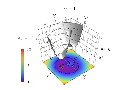
Figure 2: 3D plot of the quasienergy surfaces $Q({\cal X},{\cal P})$ for ${\cal P}>0$ and $f/g=0.154$ (Note that this yields an effective temperature of $T_{\rm eff}=0.65$, see text). The quasienergy surface for the dressed spin orientation $e$ ($\sigma_{z}=+1$) is a monostable reversed cone. The one for the opposite dressed spin $g$ ($\sigma_{z}=-1$) is bistable and is shown as a density plot as well. In the density plot, the oriented black solid line indicates the separatrix between the two domains of attraction.

Thus, we can interpret $\lambda$ as a rescaled effective Planck constant, ${\cal X}$ and ${\cal P}$ as canonically conjugated operators and $Q({\cal X},{\cal P})$ as two quasienergy surfaces in phase space for the two opposite dressed spin orientations. They are visualized in Fig. 2. The quasienergy surface for the dressed spin $g$ ($\sigma_{z}=-1$) has the overall shape of a Mexican hat. The drive induces a finite tilt of the surface, generating a saddle point at ${\cal P}_{\rm sad}=0$ and ${\cal X}_{\rm sad}=(1-f/g)/\sqrt{2}$ and a separatrix, shown in the density plot in Fig. 2 as the oriented black solid line. It divides the surface into three domains: i) a potential well around the quasienergy minimum at ${\cal P}_{\rm min}=0$ and ${\cal X}_{\rm min}=-(1+f/g)/\sqrt{2}$, ii) an internal dome around the inner maximum at ${\cal X}=0,{\cal P}=0$ and, iii) an external surface. For quasienergies lying above the saddle point and below the maximum, there are orbits coexisting on the domains ii) and iii) and thereby define a dynamical bistability. The surface for the opposite dressed spin orientation $\sigma_{z}=+1$ is a less interesting monotonous function and is shown in the 3D plot in Fig. 2.

When the motion is quantized, the (quasi-)energy levels become discrete. For small $\lambda$, we expect the dynamical behaviour to be semiclassical and we can associate each quasienergy level to an allowed orbit. In principle, a full WKB treatment is possible but it goes beyond the scope of this paper. In order to illustrate the semiclassical features of the driven Jaynes-Cummings model, we show the quasienergy levels (rescaled by $\lambda/\delta\omega$) as a function of $\lambda$ in Fig. 3. They are obtained by numerically diagonalizing the complete Jaynes-Cummings Hamiltonian.

We can associate the levels below the quasienergy saddle point $Q({\cal X}_{\rm sad},0)=-(1-f/g)^{2}/4$ (indicated in Fig. 3 as a green dotted line) to orbits localized in the quasipotential well. Notice that close to the minimum $Q({\cal X}_{\rm min},0)=-(1+f/g)^{2}/4$, the orbits are approximately equally spaced and they become denser while approaching the saddle point. In fact, semiclassically the level spacing is given by $\lambda\omega(q)$, where $\omega(q)$ is the classical orbit frequency for the (rescaled) quasienergy $q$. Close to the quasienergy minimum the potential is harmonic and $\omega(q)$ varies slowly while close to the saddle point, it tends quickly to zero.

For energies above the saddle point and below the maximum, we can associate the quasienergy levels with orbits in the internal dome and in the external surface. The orbit with vanishing quasienergy corresponds to an orbit close to the quasienergy maximum. For certain discrete values of $\lambda$, an orbit on the external surface might have vanishing quasienergy as well. Hence, we can interpret the multiphoton transitions, which occur at the resulting avoided level crossings, as tunneling transitions between two states in the internal dome and the external well, respectively. In the limit of $g\gg f$, we can read off the resonant tunneling condition from the perturbative result in Eq. (5), yielding the condition for $N$-photon transitions to be $\lambda=1/N$. More tunneling transitions for negative quasienergy are indicated by the orange circle in Fig. 3.

Above the minimum no avoided level crossing is present, several exact crossings (not shown) appear instead. The corresponding orbits have opposite dressed spin and do not show level repulsion because the two quasienergy surfaces are effectively decoupled.

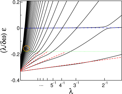
Figure 3: Rescaled quasienergy spectrum of the driven Jaynes-Cummings Hamiltonian in Eq. (2) for the parameters $f/g=0.154$ (solid black lines). The green dotted line indicates the saddle point quasienergy. The red dashed lines correspond to the approximate $(\lambda/\delta\omega)E_{n}$, see text. The blue dotted-dashed line marks the rescaled quasienergy $\varepsilon_{0}$ of $|0(f)\rangle$. The orange circle highlights avoided quasienergy level crossings (multiphoton transitions) for large photon numbers $N$.

III.1 Quasienergy states at the well bottom

Next, we study the spectrum close to the bottom of the quasienergy well quantitatively. In fact, as it turns out, the states localized in this region play an important role in the stationary dissipative dynamics close to a multiphoton transition.

The most simple approach consists in expanding the quasienergy in Eq. (11) close to its minimum. In this region, the quasienergy surface is to lowest order harmonic and follows

$$Q({\cal X},{\cal P}) = Q({\cal X}_{\rm min},{\cal P}_{\rm min})+\frac{1}{2m_{\rm eff}}({\cal P}-{\cal P}_{\rm min})^{2}$$ (13)

$$+\frac{1}{2}m_{\rm eff}{\omega^{*}}^{2}({\cal X}-{\cal X}_{\rm min})^{2}\,,$$

with effective mass $m_{\rm eff}=(f+g)/f$ and with frequency $\omega^{*}=\sqrt{f/(f+g)}$. When the zero point energy $\lambda\omega^{*}/2$ is much smaller than the quasienergy well depth $\Delta Q\equiv Q({\cal X}_{sad},{\cal P}_{sad})-Q({\cal X}_{min},{\cal P}_{min})=f/g$, only a few quasienergy states are localized in the well. The harmonic expansion yields the quasienergies

$$E_{n}=\delta\omega\lambda^{-1}\left[Q({\cal X}_{min},0)+\lambda\omega^{*}\left(n+\frac{1}{2}\right)\right]\,,$$ (14)

which are determined up to ${\cal O}(\lambda^{2})$ note2 . They are shown in Fig. 3 as red dashed lines and they almost coincide with the exact results for small $\lambda$.

Up to leading order in $\lambda$, the corresponding wave functions are given by

$$|\psi^{*}_{n}\rangle=R^{-1}\frac{b^{\dagger n}}{\sqrt{n!}}D({\cal X}_{min})S(r^{*})|0\,g\rangle\,.$$ (15)

They are obtained by applying to the vacuum: i) the squeezing operator $S(r^{*})=\exp\left[r^{*}(a^{2}-a^{\dagger 2})/2\right]$ with squeeze factor

$$r^{*}=\frac{\ln[m_{\rm eff}\omega^{*}]}{2}=\frac{\ln[1+g/f]}{4}\,,$$ (16)

ii) the translation $D({\cal X}_{\rm min})=\exp\left[i{\cal P}{\cal X}_{\rm min}/\lambda\right]$ to the minimum, iii) the creation operator $b^{\dagger}=a^{\dagger}\cosh{r}+a\sinh{r}-e^{r}{\cal X}_{\rm min}/\sqrt{2\lambda}$, and iv) $R^{-1}$ to return to the bare qubit picture. With this, one can compute the Fock-state representation yuen of the quasienergy states and all expectation values at leading order.

III.2 Quantum squeezed state and sub-Poissonian statistics

Of particular interest is the state $|\psi^{*}_{0}\rangle$ at the bottom of the quasienergy well. It is defined, when the zero point energy $\lambda\omega^{*}/2$ is smaller than the quasienergy depth $\Delta Q=f/g$, corresponding to the region $\delta\omega<g\sqrt[4]{f/g}$ ($=0.016$ for the parameters used in Fig. 1). Note that the analytical result for $E_{0}$ in Eq. (14) almost coincides with the exact one in this region. Most importantly, $|\psi^{*}_{0}\rangle$ exists for any finite driving (providing that the detuning is small enough), and is clearly absent in the undriven case. In fact, for $f=0$, the tilt of the quasienergy surface vanishes and no quasienergy well is developed. This illustrates further that simple perturbation theory fails for arbitrary small driving close to zero detuning and improves the estimate of the critical detuning below which it breaks down.

For weak but finite driving, the well is still very shallow in the momentum direction, allowing for large momentum fluctuations of a state confined in it. For increasing driving, the well becomes deeper and more symmetric. Hence,$|\psi^{*}_{0}\rangle$ is amplitude squeezed and the squeezing decreases for increasing driving, as it can also be read off from Eqs. (15) and (16).

As a consequence, $|\psi^{*}_{0}\rangle$ has also sub-Poissonian statistics and shows photon antibunching. This can be seen by computing its average photon number $\bar{n}^{*}\equiv\langle\psi^{*}_{0}|n|\psi^{*}_{0}\rangle$ and its variance $(\Delta n^{*})^{2}\equiv\langle\psi^{*}_{0}|(n-\bar{n}^{*})^{2}|\psi^{*}_{0}\rangle$ by means of Eq. (15). We find

$$\bar{n}^{*}=\frac{{\cal X}_{\rm min}^{2}}{2\lambda}=\frac{(f+g)^{2}}{4\delta\omega^{2}}\,,$$ (17)

and

$$(\Delta n^{*})^{2}=e^{-2r^{*}}\bar{n}^{*}=e^{-2r^{*}}\frac{(f+g)^{2}}{4\delta\omega^{2}}\,.$$ (18)

Thus, in the semiclassical limit $\lambda\to 0$, the $2$-photon correlation function becomes

$$g^{(2)}(0)\equiv 1+\frac{(\Delta n^{*})^{2}-\bar{n}^{*}}{\bar{n}^{*2}}<1\,,$$ (19)

Note that the above formulas can be regarded only as leading-order estimates, because they are of order $1/\lambda$ and other finite contributions are not taken into account.

Here, we did not include the Fock representation of the semiclassical states because it is rather cumbersome and scarcely illuminating for the purpose of this work. However, it is important to keep in mind that the semiclassical states are a superposition of dressed Fock states with a given dressed spin orientation and photon number $n$ of the order of $\bar{n}$, given in Eq. (17). For the discussion of the dissipative dynamics below, we remark that close to a $N$-photon transition, all the dressed Fock states that contribute significantly to the superposition correspond a photon number $n<N$ with negative quasienergies, $\varepsilon_{n<N-}<0$.

Finally, we note that the Golden Rule estimate for the rate for coherent spin flip transitions yields zero, because no overlap between the quasienergy states localized in the well (which has negative quasienergy $E_{n}<0$) and that with opposite spin (which has positive quasienergy $\varepsilon_{n+}>0$) exists.

In this work we consider identical resonant frequencies for the qubit and the cavity. However close to the quasienergy minimum the effect of a finite detuning $\delta=\omega_{\rm q}-\omega_{\rm c}$ of the resonant frequencies $\omega_{\rm q}$ and $\omega_{\rm c}$ for the qubit and the cavity might be negligible even if the circuit cavity QED is in the dispersive regime when few photons are present. The detuning $\delta$ induce an additional term $\delta^{2}\lambda/(4g^{2})$ inside the square root in Eq. (11). This further contibution is negligible close to the well bottom, if $\delta^{2}\lambda/g^{2}\ll 2{\cal X}_{\rm min}^{2}=(1+f/g)^{2}$. Note that this condition can be fullfilled even if $\delta\gg f,g$ as in Refs. Scholkopf ; Girvin . In this references, the state $|\psi^{*}_{0}\rangle$ has been denoted as bright state.

III.3 Dark state and multiphoton transitions

Another state playing a key role in the dissipative dynamics is the state obtained by starting in the JC groundstate $|0,g\rangle$ and by adiabatically switching on the driving. This is the state with zero quasienergy and is shown as blue dotted-dashed line in Fig. 3. We denote it as $|0(f)\rangle$. It is naturally favored by photon leaking, the most important dissipation channel in many set-ups. For weak driving, it has vanishing average photon number and therefore it is not accurately described by our semiclassical approach.

This state has been investigated in Ref. Milburn, for $\delta\omega=0$. It is a squeezed state which tends to follow the driving by rotating its spin by the angle $\theta\equiv\arcsin f/g$ around the the $y-$axis and squeezing its amplitude fluctuations with squeezing factor $r_{0}=-[\ln(1-f^{2}/g^{2})]/4$ Milburn . Note that, as opposed to $r^{*}$ (the squeezing factor of $|\psi^{*}\rangle$), $r_{0}$ increases for increasing driving. In addition, it has super-Poissonian statistics and shows photon bunching. In fact,

$$\bar{n}_{0} \equiv \langle 0(f)|n|0(f)\rangle_{f}=\sinh^{2}r_{0}\,,$$ (20)

$$(\Delta n_{0})^{2} \equiv \langle 0(f)|(n-\bar{n}_{0})^{2}|0(f)\rangle=2\cosh^{2}r_{0}\sinh^{2}r_{0}\,.$$ (21)

and the $2$-photon correlation function is

$$g^{(2)}(0)\equiv 1+\frac{(\Delta n)^{2}-\bar{n}}{\bar{n}^{2}}>1\,.$$ (22)

Since it is not possible to diagonalize analytically the driven JC Hamiltonian for $\delta\omega=0$, a systematic perturbation theory in $\delta\omega$ is not possible. Fortunately, for weak driving, we can rely on perturbation theory in the driving $f$ to study this state. Away from a multiphoton transition, we can compute the transmission $\langle 0(f)|a|0(f)\rangle$ by ordinary perturbation theory in $f$, yielding

$$\langle 0(f)|a|0(f)\rangle\simeq-\frac{f}{4}\left(\frac{1}{\delta\omega+g}+\frac{1}{\delta\omega-g}\right)\,.$$ (23)

Hence, the oscillation of the transmission is in phase with the driving for $\delta\omega<g$.

At a multiphoton transition, i.e, for $\lambda\approx 1/N$, the corresponding multiphoton state is a superposition of $|0(f)\rangle$ and a semiclassical state $|N(f)\rangle$, which exists on the external part of the quasienergy surface. This state is obtained by starting from a dressed state $|\phi_{N+}\rangle$ ($|\phi_{N-}\rangle$ for $\delta\omega>0$) and switching on adiabatically the driving. The states $|0(f)\rangle$ and $|N(f)\rangle$ display Rabi oscillations. The corresponding Rabi frequencies can be computed by means of Van Vleck perturbation theory as

$$\Omega_{1}=\frac{f}{\sqrt{2}},\,\,\Omega_{2}=\sqrt{2}\frac{f^{2}}{g},\,\,\Omega_{3}=\frac{3^{7/2}}{2^{4}}\frac{f^{3}}{g^{2}}\,\cdots$$ (24)

We do not give the general formula because it is rather cumbersome and scarcely illuminating. In fact, it is derived assuming that perturbation theory is valid everywhere in the spectrum, which is generally not true, not even for $f\ll g$. Our approach does not allow a fully-fledged semiclassical calculation of the Rabi frequency. Nevertheless, one main advantage is that it describes very elegantly how the physical quantities are rescaled while the effective Planck constant changes. With this, we postulate that the Rabi frequency follows as

$$\Omega_{N}\sim\exp{\left[-S(f/g)/\lambda\right]}=\exp{\left[-NS(f/g)\right]}\,.$$ (25)

with $S(f/g)$ being an unknown function of $f/g$ and $\sim$ indicating logarithmic precision.

IV Dissipative dynamics

State-of-the-art nanocircuit QED set-ups Wallraff ; Chiorescu ; Winger ; Bishop are characterized by weak damping, implying large quality factors of the order of $Q\sim 10^{4}-10^{5}$ and qubit dephasing and relaxation times ($T^{*}_{1}$ and $T_{2}$) being large compared to the timescale $T_{r}=2\pi/\omega_{r}$, governing the system dynamics. For instance, for the transmon architecture reported in Ref. Bishop, , $T_{1,2}\sim 1\mu$s and $T_{r}\sim 1$ ns. For optical cavities, quality factors of $Q\sim 10^{10}$ are possible Haroche . When decoherence and dissipation are induced by electromagnetic environmental fluctuations with a smooth spectral density and when all the time scales governing the different dissipative processes exceed typical bath-intrinsic correlation times, a Markovian dynamics is expected. The simplest Markovian master equation (MME) for the reduced density operator $\rho(t)$ of the qubit-plus-oscillator system is of Lindblad form and incorporates oscillator relaxation, qubit dephasing and qubit relaxation. Its standard form is given by $\dot{\rho}={\cal L}[\rho]$, with the Liouvillian

$${\cal L}[\rho] \equiv -i[H,\rho]+\kappa{\cal D}[a]+\gamma_{1}{\cal D}\left[\sigma_{-}/2\right]+\frac{\gamma_{\varphi}}{2}{\cal D}\left[\sigma_{z}\right],\quad$$ (26)

where ${\cal D}[O]$ is the Lindblad damping superoperator ${\cal D}[O]\equiv([O\rho,O^{\dagger}]+[O,\rho O^{\dagger}])/2$. The three damping terms describe: i) the photon leaking out of the oscillator at rate $\kappa$, ii) intrinsic qubit relaxation at rate $\gamma_{1}$, and iii) pure qubit dephasing at rate $\gamma_{\varphi}$. This phenomenological master equation follows by modelling the environment as three independent harmonic baths, each held at thermal equilibrium at the same temperature $T$, provided that $\hbar\kappa,\hbar\gamma_{1},\hbar\gamma_{\varphi}\ll k_{\rm B}T,\hbar\omega_{r}$. In Eq. (26), we have implicitly assumed a one-sided cavity with a single input and a single output port, yielding a single dissipative channel for the cavity. For a detailed description of a nanocircuit and an optical set-up implementing this model, we refer the reader to Ref. Bishop, and Ref. Thomson, , respectively.

Moreover, one has to assume $k_{B}T\ll\hbar\omega_{r}$. This condition together with the ordinary assumptions for the RWA ($\delta\omega,g,f\ll\omega_{r}$) implies that the environment acts as a perfect energy sink. However, quasienergy and not energy is the good quantum number for driven systems. Since the quasienergy is defined in a rotating frame, energy emission in a static frame (energy leaking into the environment) can appear as quasienergy absorption in the rotating frame. This leads to counterintuitive effects, such as the Unruh effect for a constantly accelerated relativistic system Unruh and quantum activation for the quantum Duffing oscillator Dykman88 . In the following, we will illustrate how our approach in terms of the quasienergy surface provides an intuitive physical insight into the dissipative dynamics even when many different quantum states are involved.

IV.1 Potential well escape: quantum activation vs. spin flips

Away from any multiphoton transition and for $g\gg f$, $|0(f)\rangle$ is characterized by a vanishing average photon number. If the system acts as an energy sink, this state has an infinitely large lifetime because a photon cannot be emitted neither from the system nor from the environment. Hence, $|0(f)\rangle$ will be dominantly populated in the stationary state. Conversely, at a multiphoton resonance, the system can escape from the $0-$photon state $|0(f)\rangle$ via resonant tunneling to the dressed $N-$photon state $|N(f)\rangle$. Subsequent relaxation causes the energy to leak out from the system via transitions to states with lower quasienergies. This leads to the occupation of all the quasienergy states with negative quasienergies. In fact, these states are a superposition of dressed Fock states with photon number $n<N$, as detailed in the previous section. Hence, when $\delta\omega<g\sqrt[4]{f/g}$, energy leaking leads to the occupation of those quasienergy states which are localized in the quasienergy well.

From the basin of attraction of the quasienergy minimum, the system can escape either i) by climbing up the quasienergy well by quantum activation, or ii) by means of a spin flip transition. In fact, only one of the two dressed spin states is confined. Hence, after a spin flip transition the system can quickly decay to the dark state. The rate $\Gamma_{a}$ for quantum activation is suppressed exponentially with the number $N_{\rm w}$ of states in the quasienergy well, following $\Gamma_{a}\propto\kappa e^{-cN_{\rm w}}$. Note that the constant $c$ does depend on the precise shape of the quasienergy surface, but not on the rescaled Planck constant $\lambda$, whereas $N_{\rm w}$ obviously depends on $\lambda$ (which governs the level spacing) according to $N_{\rm w}\propto 1/\lambda$. Hence, spin flip transitions are the dominant escape channel when $\lambda$ is small.

The stationary state is a statistical mixture of all those quasienergy states with negative quasienergy, if the overall rate of escape from the quasipotential well is of the same order as the rate of escape from the state $|0(f)\rangle$. The latter is discussed in the next subsection.

IV.2 Coherent vs. incoherent resonant dynamical tunneling

Driving may also induce resonant transitions between the qubit dressed states. To be more precise, we have to distinguish between the regimes of (A) coherent and (B) incoherent resonant dynamical tunneling. The borderline between these two regimes is determined by the ratio $\Omega_{N}/\Gamma_{N}$, where $\Omega_{N}$ is the Rabi frequency of the $N-$photon transition and $\Gamma_{N}$ is the inverse lifetime of the dressed $N-$photon state. The latter is of the order of the maximum of $N\kappa,\gamma_{1},\gamma_{\phi}$.

(A) Coherent resonant dynamical tunneling is characterized by the decay rate of the dressed $N-$photon state being smaller than the Rabi frequency, $\Gamma_{N}<\Omega_{N}$. Then, the system coherently tunnels back and forth with the Rabi frequency $\Omega_{N}$ several times before it significantly relaxes with decay rate $\Gamma_{N}/2$. All the subsequent dissipative transitions occur on a time scale similar to $\Gamma_{N}$. Therefore, the stationary solution will be a statistical mixture of all the states with negative quasienergies. This is qualitatively different from the situation away from resonance where only the $0$-photon state is significantly populated.

(B) Incoherent resonant dynamical tunneling occurs when the decay rate of the $N-$photon dressed state exceeds the Rabi frequency, $\Gamma_{N}>\Omega_{N}$. Then, the quasienergy level broadening is larger than the coherent splitting of the two quasienergy levels. The dressed $N-$photon state strongly fluctuates on a quasienergy range $\Gamma_{N}$ and with it the quasienergy difference to the $0-$photon state. Tunneling occurs only for those splittings which do not exceed the Rabi frequency $\Omega_{N}$. This occurs with probability $\Omega_{N}/\Gamma_{N}$. When the two levels are quasi-degenerate, a tunneling event then happens with probability $\Omega_{N}$. For incoherent resonant dynamical tunneling, the total tunneling probabilty is just the product of the two. Hence, the system can escape from the $0-$photon state $|0\,g\rangle$ with a small total rate $\Omega_{N}^{2}/\Gamma_{N}$. In the incoherent regime, again two situations can arise:

(B1) When no state is localized in the quasienergy well (which roughly occurs for $\delta\omega>g\sqrt[4]{f/g}$, see above), i.e., when perturbation theory in the driving $f$ is valid, the lifetimes of all the states visited during the relaxation transition are of the same order, namely of the order of $\Gamma_{N}^{-1}$. This is given by the maximum of $\kappa^{-1},\gamma_{1}^{-1},\gamma_{\phi}^{-1}$. This, however, is in any case much smaller than the lifetime of the $0$-photon state, given by $\Gamma_{N}/\Omega_{N}^{2}$ (remember that $\Gamma_{N}$ is suppressed exponentially with $N$). Thus, the $0$-photon state is maximally populated.

(B2) In the second case, when several states are trapped in the quasienergy well (which occurs for $\delta\omega\ll g\sqrt[4]{f/g}$), i.e., when the semiclassical description is necessary, the rate for quantum activation $\Gamma_{a}$ is exponentially small and can be of the order of $\Omega_{N}^{2}/\Gamma_{N}$. If also the spin flip rate is small, the state at the well bottom can become metastable. In this case, it is therefore possible that an overall small rate of incoherent resonant dynamical tunneling leads to a dramatic change in the stationary distribution as compared to the situation away from resonance, resembling the situation of coherent resonant dynamical tunneling. Note that, this will be the case only for the first few resonances. In fact the resonant escape from the dark state is suppressed exponentially with $N$, which is not the case for the spin flip escape from the bright state.

V Nonlinear response in the strong coupling regime

Having discussed all required ingredients, we can next turn to the nonlinear response of the driven JC model, which can be characterized by the steady-state expectation value of the intracavity field operator related to

$$\langle a\rangle={\rm tr}(\varrho a)=Ae^{i\varphi}=\sum_{\alpha\beta}\varrho_{\alpha\beta}a_{\beta\alpha}\,.$$ (27)

The indices $\alpha,\beta$ refer to the basis of eigenstates of the driven JC Hamiltonian in Eq. (2). In a one-sided cavity, its modulus $A$ is related to the transmitted amplitude $A_{\rm tr}\propto A$ and intensity $I_{\rm tr}\propto A^{2}$ of the input signal in a heterodyne measurement set-up Bishop ; Thomson .

These quantities are directly accessible in the experiment. In the rotating frame, $\langle a\rangle<0$ corresponds to an oscillation out of phase ($\varphi=\pi$) with respect to the drive, while the in-phase oscillation ($\varphi=0$) is associated to $\langle a\rangle>0$. Note that $\delta\omega\to-\delta\omega$ and $\varrho_{\alpha\beta}\to\varrho^{*}_{\alpha\beta}$, since the unitary transformation $\exp{[-i\pi a^{\dagger}a]}$ yields ${\cal L}\to{\cal L}^{*}$ . Moreover, $a_{\beta\alpha}\to-a_{\beta\alpha}$ and all matrix elements are real. We can conclude that the nonlinear response for $\delta\omega<0$ follows trivially from the one for $\delta\omega>0$ according to $\langle a\rangle\to-\langle a\rangle^{*}$, i.e. $A\to A$ and $\varphi\to\pi-\varphi$. In addition, due to the RWA, the master equation can be written in terms of the ratios $f/g$, $\kappa/g$, $\gamma_{1}/g$ , $\gamma_{\phi}/g$ and $\lambda$ only. Thus, also $\langle a\rangle$ depends only on these quantities.

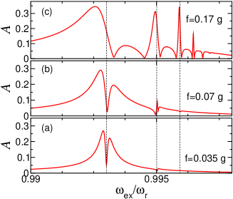
Figure 4: Nonlinear response of the driven JC model: amplitude $A$ as a function of the driving frequency $\omega_{ex}$ for $f=0.035g$ (a), $f=0.071g$ (b) and $f=0.17g$ (c). Moreover, $\kappa=6.1\times 10^{-3}g$, $\gamma_{1}=1.4\times 10^{-3}g$, $\gamma_{\phi}=1.4\times 10^{-4}g$, $g=0.007\omega_{\rm r}$. A realistic value for $\omega_{\rm r}/(2\pi)$ is $7$ GHz Bishop ; Houck .

A straightforward numerical solution of the stationary limit $\dot{\rho}(t)=0$ allows to numerically calculate the modulus $A$ as a function of the external modulation frequency $\omega_{\rm ex}$. The result for experimentally realistic parameters Bishop is shown in Fig. 4. For weak modulation, two large fundamental (anti)resonances appear symmetrically with respect to $\omega_{\rm ex}=\omega_{\rm r}$, which mark the supersplitting of the vacuum Rabi resonance (in Fig. 4a, we show only the regime of $\omega_{\rm ex}<\omega_{\rm r}$). These largest resonances (which are in fact antiresonances) are associated to the $1$-photon transitions. They can be described Bishop ; Peano3 by an effective two-level model involving the $0$- and the $1$-photon state only. At resonance, both states are equally populated and oscillate with opposite phase. This overall yields zero response exactly at resonance. Slightly away from resonance, one of the two states is slightly more populated and a finite response arises. Further away from the resonance, the response again approaches zero as discussed above (see below for a quantitative evaluation). Hence, overall, the lineshape of an antiresonance arises. The $1$-photon transitions are special situations since only two quasienergy states are involved and no contributions of other quasisenergy states with smaller photon numbers exist. Increasing the modulation strength, further resonances and antiresonances appear, see Fig. 4 b) and c). The antiresonances turn into resonances when the driving is further increased.

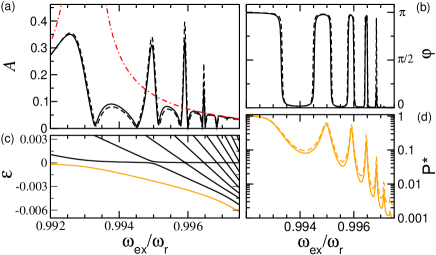
Figure 5: Solid lines: Nonlinear response of resonator in the circuit QED setup based on the transmon architecture as realized in Ref. Bishop, , i.e., $\omega/(2\pi)=6.920$ GHz, $g/\pi=94.4$ MHz, $\kappa/(2\pi)=300$ kHz, $f/(2\pi)=8.304$ MHz, $\gamma_{1}/(2\pi)=98$ kHz and $\gamma_{\phi}=0$. Dashed lines: same parameters, but without direct qubit relaxation ($\gamma_{1}=0$). Shown are (a) the amplitude $A$, (b) the phase $\phi$, (c) the quasienergy spectrum, and (d) the population $P^{*}$ of the lowest quasienergy state $|\psi_{0}^{*}\rangle$. The red dot-dashed line in (a) shows the result for the population of the $0$-photon state being assumed as close to one, see text.

In order to illustrate the underlying mechanism, we show another example of the modulus $A$ (Fig. 5a) and the phase $\varphi$ (Fig. 5b) of the oscillator response, together with the associated quasienergy spectrum (Fig. 5c) and the occupation probability $P^{*}$ of the state $|\psi_{0}^{*}\rangle$ with lowest quasienergy (Fig. 5c). For the solid lines in Fig. 5, we have chosen the same parameters as in the fits of Ref. Bishop, . As it turns out, in this experiment, the qubit pure dephasing is negligible ($\gamma_{\phi}=0$). We have also plotted (dashed lines) the case of pure Purcell dissipation (no intrinsic qubit relaxation $\gamma_{\phi}=0$, $\gamma_{1}=0$, only finite resonator damping).

First of all, we confirm that the resonances and antiresonances occur in correspondence with the avoided crossings in the spectrum. As already discussed in the previous section, in absence of resonant tunneling, i.e., away from any resonance, the occupation probability of the $0$-photon state is close to one (under the conditions discussed above), i.e., $\rho_{00}\simeq 1$. Then, from Eq. (23) follows that $\langle a\rangle\approx a_{00}=\langle 0(f)|a|0(f)\rangle$, which is shown as red dashed line in Fig. 5a). The first antiresonance occurs for $\omega_{\rm ex}=\omega_{r}-g$ and has already been discussed above. Figs.  5a) also shows the $2-,3-,4-$photon resonances and the $5-,6-$photon antiresonances. The overall phase of the stationary oscillations changes in presence of a resonance (Figs.  5b), which points to a significant population of a state oscillating out of phase. In fact, the occupation probability $P^{*}$ of the state $|\psi_{0}^{*}\rangle$ with lowest quasienergy displays peaks at such resonant frequencies, see Fig. 5d).

This phenomenology is consistent with the picture of the dissipative dynamics drawn in the previous section. At a multiphoton resonance, in presence of coherent resonant dynamical tunneling or when the rate of incoherent resonant dynamical tunneling is of the order of the rate for an escape from the quasienergy well, a sizeable occupation probability of the states confined in the quasipotential well results. Those quasienergy states oscillate out of phase and with a large amplitude, yielding peaks in the nonlinear response and an overall out-of-phase response characteristics. In the opposite limit of incoherent resonant dynamical tunneling and when no deep quasienergy well exists (i.e., in the perturbative regime) or when the escape rate is smaller than the incoherent tunneling rate, the $0$-photon state is again dominantly populated and a small but finite occupation probability of at least one state oscillating out of phase leads to a reduction of the resonant nonlinear response and thus to a dip in the lineshape, but does not necessarily change the phase. We note that the underlying mechanism is exactly the same as for the multiphoton transitions in the quantum Duffing oscillator Peano1 ; Peano2 ; Peano3 .

VI Purcell-limited set ups

The comparison of the solid and dashed lines in Figs. 5a, b, d) shows that a weak intrinsic coupling of the qubit to the environment does not change the underlying physics qualitatively. In particular, transmon qubits are Purcell-limited in the resonant regime Houck . It is therefore interesting to consider the special case of pure Purcell dissipation $\gamma_{1}=\gamma_{\phi}=0$. In this limit, the dissipative dynamics is governed by the simplified Liouville operator

$${\cal L}[\rho] \equiv -i[H,\rho]+\frac{\kappa}{2}([a\rho,a^{\dagger}]+[a,\rho a^{\dagger}]).$$ (28)

We distinguish between two different regimes: i) when only few photons are exchanged and no state is localized in the quasienergy well, a perturbative analysis (in the driving) is in order. ii) In the opposite case, our physical picture in terms of quasienergy surfaces is necessary to discuss the dissipative dynamics.

VI.1 Small photon number: perturbative regime

When no state is localized in the quasienergy well and away from a any multiphoton resonance, the quasienergy levels match the unperturbed result of Eq. (3) and the corresponding states can be identified with the dressed states $|\phi_{n-}\rangle$.

Close to the $N-$photon resonance, two scenarios are possible, as discussed above: (A) coherent resonant dynamical tunneling (i.e., when the lifetime $\Gamma_{N}$ of the $N-$photon state $|\phi_{N\pm}\rangle$ is much smaller than the Rabi frequency $\Omega_{N}$), and, (B) incoherent resonant dynamical tunneling (i.e., when $\Gamma_{N}\gg\Omega_{N}$).

When the dynamical tunneling is coherent ($\Gamma_{N}\ll\Omega_{N}$), the system tunnels many times between the states $|\phi_{0}\rangle$ and $|\phi_{N-}\rangle$ with period $2\pi/\Omega_{N}$ before it substantially decays to $|\phi_{N-1-}\rangle$. The rate of this decay can be obtained in secular approximation as $\Gamma_{N}/2=\kappa(N-1/2)/2$. Subsequent decays from $|\phi_{n-}\rangle$ to $|\phi_{n-1-}\rangle$ occur along the ladder $N-1\to N-2\to...\to 1\to 0$ with decay rates ${\cal D}_{n-,(n-1)-}=(\sqrt{n}+\sqrt{n-1})^{2}\kappa/4$ for $n\neq 1$ and ${\cal D}_{1-,0}=\kappa/2$. Hence, the rate from the $1$-photon to the $0$-photon state is smallest. Note that the probability of a decay to a state with opposite dressed spin is small, i.e., ${\cal D}_{(n-1)-,n+}/{\cal D}_{(n-1)+,n+}\simeq 1/[16n\left(n-1/2\right)]$. Thus, in this scenario, the occupation probability of $\rho_{11}$ is the largest. It can be computed (once the spin-flips are neglected) by straightforwardly solving the master equation, which yields

$$\rho_{11}=\left(1+f^{-2}_{+}(N)+\sum_{n=2}^{N-1}\frac{f^{-2}_{+}(n)}{2}\right)^{-1}\,,$$ (29)

where $f_{+}$ is defined below Eq. (III). Therefore, the contribution $\rho_{11}a_{11}$ with

$$a_{11}=\frac{f}{2(\varepsilon_{1-}-\varepsilon_{2-})}\frac{3+2\sqrt{2}}{4}+\frac{f}{4(\varepsilon_{1-}-\varepsilon_{0})}$$ (30)

is the largest in Eq. (27). For all multiphoton transitions with photon number $N<6$, $\varepsilon_{1-}<\varepsilon_{2-},\varepsilon_{0}$, resulting in the contribution $\rho_{11}a_{11}<0$ and thus in an overall stationary oscillation which is out of phase with the modulation.

In the example considered in Fig. 6 ($f=0.057g$, $\kappa=0.0009g$ and $g=0.007\omega_{r}$), this scenario is realized close to the $2-$photon transition. The ratio between the $2-$photon Rabi frequency $\Omega_{2}=\sqrt{2}f^{2}/g$ (see Eq. (24)) and the lifetime of the $2-$photon dressed state $\Gamma_{2}=3/2\kappa$ is $\Omega_{2}/\Gamma_{2}=(2\sqrt{2}/3)f^{2}/(g\kappa)=3.4$ and the tunneling is coherent. As expected, the overall behavior changes from an in-phase oscillation with amplitude $|a_{00}|$ (red dashed line in Fig. 6) to a larger out-of-phase oscillation of the order of $|a_{11}|$ (blue dotted line). Moreover, the occupation probability $\rho_{11}$ displays a peak (Fig. 6d), whose height is close to the approximate value computed in Eq. (29). It is represented as a blue star in Fig. 6d).

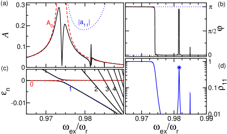
Figure 6: Nonlinear response of the driven JC model: (a) amplitude, (b) phase, (c) quasienergies, and (d) population of the lowest quasienergy state for $f=0.057g,\kappa=0.0009g$ and $g=0.026\omega_{\rm r}$. Dashed red (dotted blue) line in (a,b,c): lowest-order result for $|0(f)\rangle$ ($|1(f)\rangle$).

In the opposite limit of incoherent resonant dynamical tunneling ($\Gamma_{N}\gg\Omega_{N}$), the population of $|\phi_{0}\rangle$ is $\simeq 1$, because relaxation to the $0-$photon state is more efficient than any escape from there via tunneling. Dissipation then completely washes out the resonance, and the response is identical to that away from resonance and thus is in phase with the drive.

In the intermediate regime when $\Gamma_{N}\simeq\Omega_{N}$, a small population $\rho_{11}$ emerges, contributing $\rho_{11}a_{11}$ with $a_{11}<0$ given in Eq. (30), which is negative for $N<6$ (in the perturbative regime). This also leads to a reduced response with an antiresonance. This scenario is realized close to the $3-$photon transition in Fig. 6). In this case, the Rabi frequency is $\Omega_{3}=(3^{7/2}/2^{4})f^{3}/g^{2}$ and $\Gamma_{3}=(5/2)\kappa$, so that $\Omega_{3}/\Gamma_{3}=0.24$.

VI.2 Large photon number: semiclassical regime

When several photons are contained in the resonator, a picture in terms of the dissipative semiclassical dynamics emerges. As will be shown below, a separation of relaxation time scales exists, which separates fast intrawell from slow interwell relaxation. We first focus on the intrawell dynamics. Close to the minimum, the wave functions are given by Eq. (15). We can compute the corresponding dissipative transition rates by plugging them into Eq. (28). In this limit, dissipative transitions occur only between nearest neighbors, with the rates ${\cal D}_{n-1,n}=\kappa n\cosh^{2}r$ and ${\cal D}_{n,n-1}=\kappa n\sinh^{2}r$. Here, the detailed balance condition is fulfilled. Hence, when the system is initially in a state with a large photon number $n$, it falls with large probability into the basin of attraction of the quasienergy minimum. This process constitutes intrawell relaxation. When furthermore damping is smaller than the intrawell level spacing, i.e., $\kappa\ll g\lambda\omega^{*}$ (see Eq. (14)), detailed balance is retained and determines an effective Boltzmann distribution

$$P^{*}_{n}=P^{*}e^{-n\beta_{\rm eff}}\,,$$ (31)

with the effective inverse temperature $\beta_{\rm eff}=2\ln\coth r^{*}$ being defined in terms of the squeezing parameter $r^{*}$. We emphasize that this link between effective temperature and squeezing can be generalized to any driven quantum system with a smooth quasienergy surface and coupled linearly to a bath (e.g., the linearly and the parametrically driven Duffing oscillator). It can be easily generalized to finite real temperatures $T>0$ as well. It turns out that the zero temperature limit applies when $\sinh^{2}r$ is much larger than the bosonic occupation number $\bar{n}(\omega_{\rm ex}/T)$ of the bath taken at frequency $\omega_{\rm ex}$. In the opposite limit, $\beta_{\rm eff}=\omega_{\rm ex}/T$. Since we include here only photon leaking, i.e., $\omega_{\rm ex}\gg T$, the effective temperature is still small.

On the large time scale, the system can escape from the basin of attraction of the quasienergy minimum with a small forward rate $k_{+}$. Overall there are two mechanism contributing to the escape: i) The system can climb up the quasienergy well by quantum activation. As already discussed in Section IV, the corresponding rate $\Gamma_{a}$ is suppressed exponentially, following $\Gamma_{a}\propto\kappa e^{-c/\lambda}$. Moreover, ii) the bath induces spin-flip transitions with rate $\Gamma_{s}$ even in absence of an intrinsic spin-bath coupling. This is a consequence of the dressing of the spin. From Eqs. (8) and (28), it follows that $\Gamma_{s}\propto\lambda$. Therefore, this mechanism is dominant for small $\lambda$ and the rate $k_{+}$ vanishes according to $k_{+}\propto\lambda$. In real set-ups, a lower bound to $k_{+}$ is given by the small intrinsic couplings $\gamma_{1}$ and $\gamma_{\phi}$ of the spin to the bath.

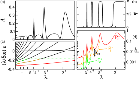
Figure 7: Nonlinear response of the driven JC model: (a) amplitude, (b) phase, (c) quasienergies, and (d) population of the lowest quasienergy states $|\psi^{*}_{n}\rangle$ ($n=0,1,2$) as a function of the rescaled Planck constant $\lambda$ for the parameters $f/g=0.171,\kappa/g=6.110^{-3}\omega_{\rm r}$, $\gamma_{1},\gamma_{\phi}=0$ (Purcell limit). Green dotted line in (c): quasienergy of the saddle point.

Once the system has left the basin of attraction of the bright state $|\psi_{0}^{*}\rangle$, it quickly decays to the dark state $|0(f)\rangle$. From there, it can escape with a backward rate $k_{-}$ on a large time scale. The stationary populations of the intrawell states, which oscillate out of phase, and the $0-$photon state, which oscillates in phase with the modulation, are determined by the ratio $k_{-}/k_{+}$. Away from any resonance, photon leaking favors the $0-$photon (dark) state and thus, the corresponding interwell relaxation is fast, i.e., $k_{+}\gg k_{-}$. Close to a resonance for $\lambda=1/N$ (N integer), if the driving is resonant or the incoherent resonant tunneling rate $k_{-}=\Omega_{N}^{2}/\Gamma_{N}$ is of the same order of $k_{+}$, the response is qualitatively modified and the resonant-antiresonant transition is now governed by the ratio $k_{-}/k_{+}$.

Next, we complete our discussion with numerical results for a concrete example. In Fig. 7, we plot (a) the overall oscillation amplitude, (b) the overall phase, (c) the rescaled quasienergy spectrum, and (d) the occupation probabilities of the first three states $|\psi^{*}_{n}\rangle$ ($n=0,1,2$) at the well bottom as a function of the effective Planck constant $\lambda$. For $\lambda\approx 1/N$ ($N=2,3,4,5$), we observe a resonant out-of-phase response (see Figs. 7 a) and b), whereas for $\lambda\approx 1/6$, an antiresonance appears which is in phase with the modulation signal. For the same values of $\lambda$, the occupation probabilities of the states in the well display peaks, see Fig. 7 d). The heights of the respective peaks are suppressed exponentially with $N$. According to the detailed balance condition in Eq. (31), the ratio of the probabilities for nearby states close to the bottom of the well is $\exp(-\beta_{\rm eff})$. In fact, in logarithmic scale, the individual curves of the probabilities tends to be equidistant. The theoretical value for the gap between the curves is shown by the black double arrow, indicating that the agreement with Eq. (31) is also quantitative.

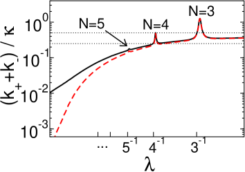
Figure 8: Solid line: Smallest eigenvalue of the Lindblad master equation. Dashed red line: the same without dissipative spin flips. Dashed-dotted orange line: decay rate for $|\psi^{*}\rangle\to|\phi_{0}^{f}\rangle$. Dotted lines correspond to $\kappa/2$ and $\kappa/4$.

In order to underpin the drawn picture by more quantitative results, it is is helpful to consider the eigenvalues of the Liouville operator. For this, we start deep in the semiclassical regime, i.e., with small detuning. Here, a clear separation of time scales for the dissipative dynamics on the bistable quasienergy surface occurs. Well-defined energy wells with a large quasienergy barrier in between exist for small detuning and allow for a clear description in terms of a single relaxation rate (see also Ref. rate, for a comprehensive review). In this regime, we find a single eigenvalue $\Gamma$ which consists of the sum of $k_{-}$ and $k_{+}$ , is real and much smaller than the real parts of all the other eigenvalues. This is shown in Fig. 8 as black solid line. In order to emphasize the role of bath induced spin-flips, we have also computed the smallest eigenvalue $\Gamma$ of the Liouvillian after removing those transition by hand from the master equation, see red dashed line in Fig. 8. For increasing $\lambda$, i.e., when $\lambda\gtrsim 0.25$, we enter a regime, where the separation of time scales is not so clearly expressed and $\Gamma$ becomes comparable to the real parts of the next three eigenvalues. The latter correspond to relaxation (one real eigenvalue) and to decoherence (a complex conjugated pair of eigenvalues), involving the pair of states $|\phi_{1+}\rangle$ and $|\phi_{0}\rangle$. We do not show them in the figure, but instead show the perturbatively determined values $\kappa/2$ (relaxation) and $\kappa/4$ (decoherence) out of resonance as dotted horizontal lines. The peaks in the total rate $\Gamma$ are due to resonant dynamical tunneling for $k_{+}$ as discussed in Section IV.2. Due to the logarithmic scale, peaks in $\Gamma$ are only visible when $k_{+}$ is of the order or larger than the background value given by $k_{-}$.

VII Connection to other models

The analysis presented here can in general be extended to any driven nonlinear oscillator coupled bilinearly to a thermal bath. For example, the Duffing oscillator is characterized by two classical stable solutions with opposite oscillation phase. In the quantum regime, two quantum squeezed states correspond to them. For weak driving, the small-oscillation solution can be identified with the $0-$photon quantum state. At low thermal energies, it is dominantly populated away from any resonance due to photons leaking into the bath. Thus, it can be regarded as stable in absence of any multiphoton transitions. However, this stable quasienergy state is associated to a relative quasienergy maximum, which is in direct contrast to the case of a static bistable potential. There, the lowest energy state is always the minimum of the true potential. At a multiphoton resonance, the zero-photon quasienergy state is no longer stable since excitations to a $N-$photon state occur. Hence, it becomes metastable and generates a (anti-)resonance of the stationary oscillation. This behavior of the quantum Duffing oscillator has been already predicted Peano1 ; Peano2 ; Peano3 , but the link to the semiclassical picture Dmitriev86 ; Dykman88 has not been drawn. Thus, the generic behavior of a driven damped nonlinear quantum oscillator includes dynamically generated metastable states from which the system can escape via thermal diffusion, quantum activation or dynamical tunneling. In the regime of many photons in the resonator, the escape rate of dynamical tunneling processes can be obtained in a semiclassical description, while in the regime of only few photons (deep quantum regime), the escape can occur via resonant dynamical tunneling, leading to resonant multiphoton transitions. Depending on the ratio of the Rabi frequency and the lifetime of the multiphoton state, the resonant dynamical tunneling can be coherent (for large quality factors) or incoherent (for small quality factors). Depending on the phase of the associated multiphoton transitions, a resonant or an antiresonant nonlinear response may arise. Such a situation is also expected in a Josephson bifurcation amplifier jba operated in the deep quantum regime (note that all related experimental setups realized so far operate in the classical regime).

VIII Conclusions

In conclusion, inspired by recent experiments, we have shown that a driven circuit QED setup can acquire a dynamical bistability. The relevant model to describe this is the driven dissipative Jaynes-Cummings model for which we have analyzed its nonlinear response properties. We have shown that a quasienergy surface can be derived in a rotating frame picture which clearly shows two metastable basins of attraction. This picture is also convenient for studying the semiclassical limit. We have predicted the existence of a metastable quantum squeezed state in the semiclassical limit and have discussed a connection between effective local temperature at the bottom of the quasienergy well and the squeezing parameter. We have analyzed the escape mechanisms from the metastable states and found resonant dynamical tunneling, both in an incoherent and a coherent version. Our analysis adds another example to the series of nonlinear driven dissipative quantum systems with surprising and counterintuitive, but generic features. The thorough experimental investigation of these intrinsic quantum effects is an interesting prospect.

- (1) A.H. Nayfeh and D.T. Mook, Nonlinear Oscillations (Wiley, New York, 1979).
- (2) M.I. Dykman and M.A. Krivoglaz, Physica A 104, 480 (1980).
- (3) M.I. Dykman and M.A. Krivoglaz, Sov. Phys. JETP 50, 30 (1979).
- (4) M.I. Dykman and V.N. Smelyanski, Phys. Rev. A 41, 3090 (1990).
- (5) A.P. Dmitriev and M.I. D’yakonov, Sov. Phys. JETP 63, 838 (1986).
- (6) M.I. Dykman and V.N. Smelyanskii, Sov. Phys. JETP 67, 1769 (1988).
- (7) M. Marthaler and M.I. Dykman, Phys. Rev. A 73, 042108 (2006).
- (8) C. Hicke and M.I. Dykman, Phys. Rev. B 76, 054436 (2007).
- (9) V. Peano and M. Thorwart, Phys. Rev. B 70, 235401 (2004).
- (10) V. Peano and M. Thorwart, Chem. Phys. 322, 135 (2006).
- (11) V. Peano and M. Thorwart, New J. Phys. 8, 21 (2006).
- (12) V. Peano and M. Thorwart, Europhys. Lett. 89, 17008 (2010).
- (13) E.T. Jaynes and F.W. Cummings, Proc. IEEE 51, 89 (1963)
- (14) J. Larson, Phys. Scr. 76, 146 (2007).
- (15) A. Wallraff et al., Nature 431, 162 (2004).
- (16) I. Chiorescu et al., Nature 431, 159 (2004).
- (17) N. Hatakenaka and S. Kurihara, Phys. Rev. A 54, 1729 (1996).
- (18) M. Winger et al., Phys. Rev. Lett. 101, 226808 (2008).
- (19) A. Blais, R.-S. Huang, A. Wallraff, S.M. Girvin, and R.J. Schoelkopf, Phys. Rev. A 69, 062320 (2004).
- (20) K. Moon and S.M. Girvin, Phys. Rev. Lett. 95, 140504 (2005).
- (21) M. Wallquist, V.S. Shumeiko, and G. Wendin, Phys. Rev. B 74, 224506 (2006).
- (22) S. Swain and Z. Ficek, J. Opt. B: Quantum Semiclass. Opt. 4, S328 (2002).
- (23) J. Hauss, A. Fedorov, C. Hutter, A. Shnirman, and G. Schön, Phys. Rev. Lett. 100, 037003 (2008).
- (24) R.J. Brecha, P.R. Rice, and M. Xiao, Phys. Rev. A 59, 2392 (1999).
- (25) L.S. Bishop et al., Nature Phys. 5, 105 (2009).
- (26) L. Tian and H.J. Carmichael, Phys. Rev. A 46, 6801 (R) (1992).
- (27) R.J. Schoelkopf and S. M. Girvin, Nature 451, 664 (2008).
- (28) R. J. Thomson, G. Rempe, and H. J. Kimble, Phys. Rev. Lett. 68, 1132 (1992).
- (29) S. Haroche and J.-M. Raimon, Exploring the Quantum, (Oxford University Press, Oxford 2006).
- (30) The terms neglected in the RWA could be taken care in the framework of Floquet theory. They are of the order of and .
- (31) P. Carbonaro, C. Compagno and F. Persico, Phys. Lett. 73 a, 99 (1979)
- (32) The contributions to the quasienergies of order from higher order terms of the quasipotential should be taken into account but cancel out.
- (33) H. P. Yuen, Phys. Rev. A 13, 2226 (1976).
- (34) M. D. Reed et al., arXiv:1004.4323
- (35) L. Bishop, E. Ginossar and S. M. Girvin, arXiv:1005.0377
- (36) G. Milburn and P. Alsing, in Directions in Quantum Optics, Lecture Notes in Physics, ed. by H.J. Carmichael, R.J. Glauber, and M.O. Scully, 561, 303 (Springer, Berlin 2001).
- (37) W. Unruh, Phys. Rev. D 14, 870 (1976).
- (38) A. A. Houck et al., Phys. Rev. Lett. 101, 080502 (2008).
- (39) P. Hänggi, P. Talkner, and M. Borkovec, Rev. Mod. Phys. 62, 251 (1990).
- (40) I. Siddiqi et al., Phys. Rev. Lett. 93, 207002 (2004).