On the suspected timing-offset–induced calibration error in the Wilkinson microwave anisotropy probe time-ordered data

Abstract

Context. In the time-ordered data (TOD) files of the Wilkinson Microwave Anisotropy Probe (WMAP) observations of the cosmic microwave background (CMB), there is an undocumented timing offset of $-25.6$ ms between the spacecraft attitude and radio flux density timestamps in the Meta and Science Data Tables, respectively. If the offset induced an error during calibration of the raw TOD, then estimates of the WMAP CMB quadrupole might be substantially in error.

Aims. A timing error during calibration would not only induce an artificial quadrupole-like signal in the mean sky map, it would also add variance per pixel. This variance would be present in the calibrated TOD. Low-resolution map-making as a function of timing offset should show a minimum variance for the correct timing offset.

Methods. Three years of the calibrated, filtered WMAP 3-year TOD are compiled into sky maps at HEALPix resolution $N_{\mathrm{side}}=8$, individually for each of the K, Ka, Q, V and W band differencing assemblies (DA’s), as a function of timing offset. The median per map of the temperature fluctuation variance per pixel is calculated and minimised against timing offset.

Results. Minima are clearly present. The timing offsets that minimise the median variance are $-38\pm 8$ ms (K, Ka), $-27\pm 3$ ms (Q), $-43\pm 8$ ms (V), and $-47\pm 194$ ms (W), i.e. an average of $-30\pm 3$ ms, where the WMAP collaboration’s preferred offset is $0\pm 1.7$ ms. A non-parametric bootstrap analysis rejects the latter at a significance of $99.999\%$. The hypothesis of a $-25.6$ ms offset, suggested by Liu, Xiong & Li from the TOD file timing offset, is consistent with these minima.

Conclusions. It is difficult to avoid the conclusion that the WMAP calibrated TOD and inferred maps are wrongly calibrated. CMB quadrupole estimates $(3/\pi)C_{2}$ based on the incorrectly calibrated TOD are overestimated by roughly $64\pm 6\%$ (KQ85 mask) to $94\pm 10\%$ (KQ75 mask). Ideally, the WMAP map-making pipelines should be redone starting from the uncalibrated TOD and using the $-25.6$ ms timing offset correction.

1 Introduction

Liu & Li (2010a) made sky maps out of the time-ordered data (TOD) files of the Wilkinson Microwave Anisotropy Probe (WMAP) observations of the cosmic microwave background (CMB) (Bennett et al. 2003b), following the procedure recommended by the WMAP collaboration. They found a considerably weaker CMB quadrupole signal than that estimated by the WMAP collaboration, but were not aware of the reason for the difference, given that their software pipeline satisfied many tests. Later, Liu et al. (2010a) found that (i) they had used a different choice of timing interpolation than that of the WMAP collaboration, and (ii) there is a timing offset of $-25.6$ ms between the spacecraft attitude and radio flux density timestamps, recorded in the Meta and Science Data Tables, respectively, in the TOD files. Individual observations in the Q, V and W bands last for 102.4 ms, 76.8 ms, and 51.2 ms, respectively (Section 3.2, Limon et al. 2010), so the offset corresponds to half of a W band observing interval or a quarter of a Q band observing interval. The 21 April 2010 version of the WMAP Explanatory Supplement (Section 3.1, Limon et al. 2010) does not refer to the $-25.6$ ms offset.

Liu et al. (2010a) presented a simple model for the effect of a timing error on subtraction of the Doppler-induced dipole signal, which is celestial-position–dependent because it is a dipole and time-dependent because of the spacecraft’s orbit around the Sun, demonstrating that an artificial quadrupole-like signal would be generated. Moss et al. (2010) presented a toy model that confirmed that a timing offset of $-25.6$ ms would induce an artificial quadrupole approximately aligned with what had been previously considered to be the cosmological CMB quadrupole signal. There was no clear consensus between Liu et al. (2010a) and Moss et al. (2010) regarding the fraction of the quadrupole that would be artificial.

If the timing offset induced an error in compiling the calibrated TOD into maps, then this should introduce a blurring effect at a few-arcminute scale. This effect would not be easy to see by eye in sky maps. However, statistically, in full-sky maps created without ignoring bright objects, the hypothesis that a timing offset introduced an error in the compilation of the calibrated TOD into maps was excluded to very high significance (Roukema 2010).

Nevertheless, this method did not exclude the possibility that a timing offset could have induced a quadrupole-like artefact during the calibration of the uncalibrated TOD. Indeed, Jarosik et al. (Section 2.4.1, Figs 3, 4, Jarosik et al. 2007) showed that an error in the gain model could lead to a quadrupole-like artefact in inferred sky maps. Although the Doppler dipole is not subtracted from the data during the calibration step, it is the signal used for the calibration itself.

In principle, it would be possible to recalibrate the uncalibrated TOD using several different values of the timing offset, remake sky maps from the newly calibrated TOD, and test a statistic of these sky maps that shows which timing offset is optimal. However, a simpler approach is possible.

A timing error during calibration would not only induce an artificial quadrupole-like signal in the mean. It would also add variance to the sky map signal per pixel. This would be present in the calibrated TOD. In other words, the effect of the error would be to add a small noise component to the signal per pixel. Since the calibrated TOD consist of individual observations, as do the uncalibrated TOD, reversing an incorrect timing offset when map-making from the calibrated TOD should approximately correct the dominant signal, the dipole, reducing this variance. Here, minimalisation of the variance per pixel, as a function of timing offset, is carried out. Maps of both $\delta T$ and $(\delta T)^{2}$ are generated from the calibrated TOD as a function of timing offset in order that variance maps can be inferred. The timing offset that gives the minimum variance should be that which is correct.

The would-be timing-offset–induced calibration error and the way that an approximate reversal of the error should reduce the per-pixel variance are explained in Sect. 2.1. A toy model illustrating the variance reduction is presented in Sect. 2.2. The observational analysis and variance minimisation method are described in Sect. 2.3. The timing offset hypotheses are summarised quantitatively in Table 1. Results are presented in Sect. 3, with the main results in Table 2. A rough estimate of the relevance of the results for the CMB quadrupole is made in Sect. 3.1. The discussion section deals with sensitivity to the fitting method (Sect. 4.1), consistency between wavebands (Sect. 4.2), the possible relevance of sidelobe and other beam effects (Sect. 4.3), consistency with the results of using an alternative method (Sect. 4.4), and various caveats (Sect. 4.5). Conclusions are given in Sect. 5. Gaussian error distributions are assumed throughout, except where otherwise stated.

2 Method

2.1 Model of would-be calibration error

The full calibration procedure is described in Hinshaw et al. (2003), along with details for the 3-year data in Jarosik et al. (2007). Calibration to the dipole signal plays a fundamental role in this procedure. The direction and amplitude of this signal vary slightly throughout the year, mainly as a result of the orbit of the WMAP spacecraft around the Solar System barycentre.

The dipole signal used in the calibration procedure includes both an estimate of the contribution from the Solar System barycentre’s motion with respect to the comoving coordinate system, and a component due to the WMAP spacecraft’s motion around the Solar System barycentre (Sect. 2.2.1 Hinshaw et al. 2003). The latter is measured to high precision, presumably as a function of a time standard, e.g. Julian days, consistent with that used in the main mapmaking procedure.

Let us suppose that a timing offset is present when calculating the dipole that is used for the calibration of one hour of TOD, i.e. the times associated with the TOD spacecraft attitude quaternions are used rather than the times associated with the TOD. Suppose that the only signal observed is that of the true dipole, and that the random errors in measurement are negligible. Over the approximately annular region corresponding to one hour’s observations, the result of the calibration will be to shift the input signal in sky position to match the dipole calculated for a slightly incorrect position. That is, the gain and baseline will be wrongly estimated by a small amount that depends on the wrongly calculated dipole expected to be present in the observed annulus, in a way that on average corresponds to a positional shift.

Over a full year, the set of observations in a given pixel (for some given pixel size) depends on the various hourly subsets of TOD of which that pixel is a member. The set of temperature fluctuation estimates in that pixel will have non-zero variance induced by the varying errors from different hourly calibrations. Thus, by calibrating with a timing offset, noise per pixel is added to observations that by assumption consist of the true dipole and negligible random measurement error.

Now suppose that we have a set of wrongly calibrated observations (TOD), retaining the assumptions that the only observed signal is the dipole and that measurement error is negligible. Consider the meaning of calibration. In any hourly subset of TOD, the measured signal is offset and scaled in such a way that it matches the calibration signal. Thus, we know what the result of wrongly calibrating the input signal is. It is the assumed dipole. Hence, the wrongly calibrated values can be corrected towards the true values by using knowledge of the scanning path, the assumed dipole, and the timing offset. This reduces the variance per pixel down towards the original, negligible measurement error. The error cannot be reduced to zero, in this simplified case, because the calibration is not carried out on individual observations (which would be meaningless), it is carried out on (usually) hourly subsets of the TOD.

This can be expressed mathematically as follows. Given errorless observations $\delta T[\phi(t),\theta(t)]$ of the dipole, the hourly calibration of these correct dipole observations to an incorrectly timed dipole is equivalent to applying the functional $g_{\mathrm{h}}\approx g$, where $g_{\mathrm{h}}$ is the functional for the hourly calibration,

$$g:\delta T[\phi(t),\theta(t)]\mapsto\delta T[\phi(t-\delta t),\theta(t-\delta t)]$$ (1)

is the functional for what would hypothetically consist of calibrating every observation individually, and the timing offset is $\delta t$. This approximation should hold because the dipole is a smooth function with features only on large scales. Thus, the wrongly calibrated TOD can be written as $g_{\mathrm{h}}(\delta T)$.

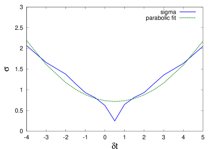
Figure 1: Minimisation of a median-per-map standard deviation per pixel $\sigma(\delta t)$ [Eq. (16)] in a realisation of a toy simulation of would-be wrongly calibrated data with an input timing offset of $\delta t=0.5$, fit by a parabola over a range of timing offsets centred at $\delta t=0.5$.

The inversion of the shift $g^{-1}$ is

$$g^{-1}:\delta T[\phi(t),\theta(t)]\mapsto\delta T[\phi(t+\delta t),\theta(t+\delta t)].$$ (2)

Thus,

$$g^{-1}\{g_{\mathrm{h}}[\delta T(\phi,\theta)]\} \approx g^{-1}\{g[\delta T(\phi,\theta)]\}$$ (3)

$$= \delta T(\phi,\theta).$$

Hence,

$$\sigma\left(g^{-1}\{g_{\mathrm{h}}[\delta T(\phi,\theta)]\}\right)\Big{|}_{\phi,\theta} \approx \sigma\left[\delta T(\phi,\theta)\right]\Big{|}_{\phi,\theta}$$ (4)

$$< \epsilon$$

$$< \sigma\left\{g[\delta T(\phi,\theta)]\right\}\Big{|}_{\phi,\theta},$$

where the variance $\sigma^{2}$ is defined for the set of observations in a pixel at a fixed position $(\phi,\theta)$. The relation $\sigma\left[\delta T(\phi,\theta)\right]\Big{|}_{\phi,\theta}<\epsilon$ is the assumption that the observations have negligible ($<\epsilon\ll 1$ in any units) measurement error. Hence, given a set of wrongly calibrated observations $\delta T^{\prime}:=g_{\mathrm{h}}(\delta T)$ of originally errorless observations $\delta T$ of the pure dipole signal, minimisation of

$$\sigma\left[g^{-1}(\delta T^{\prime})\right]\Big{|}_{\phi,\theta}$$ (5)

as a function of $\delta t$ should yield the timing offset implicit in the wrong calibration.

In reality, the signal is not expected to be a pure dipole signal, and the measurements are not errorless. Moreover, an iterative procedure involving both calibration and mapmaking is used to optimise the calibration procedure (Sects 2.2, 2.3, Hinshaw et al. 2003), and a more complex gain model is used in the calibration of the 3-year data (Sect 2.4, Jarosik et al. 2007). Thus, some additional error will be introduced into the above minimisation by the complex calibration procedure.

Another potential complication is that use of $g^{-1}$ will also induce a blurring effect at small (arcminute) scales (Roukema 2010, and references therein). At this small scale, application of $g^{-1}$ should increase the variance per pixel if the dipole is assumed to be constant on this scale. Hence, in order to detect the original calibration error, a large enough pixel size must be used so that the dominant contribution to the variance per pixel is from positional offsets to the dipole rather than from blurring of point sources.

2.2 Toy model

A toy model illustrating the detection of a timing offset by minimising the variance per pixel can be set up as follows. Consider a fixed map vector $m$ of $N_{\mathrm{pix}}$ pixels, composed of a fixed sinusoidal “dipole” map (a one-dimensional simplification of a dipole) defined

$$m_{\mathrm{0}}(j):=3\sin\left(2\pi\frac{j}{N_{\mathrm{pix}}}\right),$$ (6)

at pixel $j$ and a component that includes CMB signal and noise, modelled (for simplicity) as Gaussian noise of zero mean and standard deviation 0.5, i.e. $m$ is pixelwise defined

$$m(j):=m_{\mathrm{0}}(j)+0.5G(0,1).$$ (7)

The units can be thought of as mK.

A TOD vector $d$ representing $N_{\mathrm{TOD}}$ successive observations during one year can now be defined via an $N_{\mathrm{TOD}}\times N_{\mathrm{pix}}$ mapping matrix $M(\delta t)$ at timing offset $\delta t$

$$d=M(\delta t)\,m+\left[M(\delta t)\cdot{M_{\mathrm{1}}(\delta t)}^{\mathrm{T}}\right]\,\mathbf{e}$$ (8)

where $\cdot$ is the Hadamard product,

$$\left[M_{\mathrm{1}}(\delta t)\right]_{ij}:=0.3\sin\left[2\pi\frac{j}{N_{\mathrm{pix}}}+2\pi\frac{i+\delta t}{N_{\mathrm{TOD}}}\right]$$ (9)

is an $N_{\mathrm{pix}}\times N_{\mathrm{TOD}}$ matrix representing the dipole component that varies during the year, and $\mathbf{e}$ is a column vector of size $N_{\mathrm{pix}}$ whose entries are 1, used for summation. The timing offset $\delta t$ may either be the correct value, in which case $M(\delta t)$ is the correct mapping matrix and $M_{\mathrm{1}}(\delta t)$ is the correct time-varying dipole, or $\delta t$ may be a guessed value.

Let the mapping matrix $M(\delta t)$ be initialised to zero. For the $i$-th TOD observation, define the first beam column number

$$j_{1}(\delta t):=$$

$$\mathrm{mod}\left\{\left\lfloor\frac{70.5}{360}N_{\mathrm{pix}}\left[\sin\left(100\pi\frac{i+\delta t}{N_{\mathrm{TOD}}}\right)+\frac{i}{N_{\mathrm{TOD}}}\right]\right\rfloor,\;N_{\mathrm{pix}}\right\},$$

(10)

where $\lfloor.\rfloor$ is the floor function, set the second beam column number

$$j_{2}[j_{1}(\delta t)]:=\mathrm{mod}\left[j_{1}(\delta t)+\left\lfloor\frac{141}{360}N_{\mathrm{pix}}\right\rfloor,N_{\mathrm{pix}}\right]$$ (11)

and set matrix elements for the two beams

$$M_{i,j_{1}(\delta t)} = 1/(1+x_{\mathrm{im}})$$

$$M_{i,j_{2}[j_{1}(\delta t)]} = -1/(1-x_{\mathrm{im}}),$$ (12)

where $x_{\mathrm{im}}=\pm 0.007$ is a differencing assmbly imbalance parameter with a randomly chosen sign in a given simulation. The motivation for these functions is to have a scanning pattern whose fractional sky coverage and fractional year coverage roughly correspond to those of the real observations, e.g. one beam varies approximately sinusoidally in addition to a linear ($S^{1}$) yearly orbit, and the second beam is separated from the first by a pixel distance of $(141^{\circ}/360^{\circ})N_{\mathrm{pix}}$.

The first and second moments of temperature fluctuation estimates calculated directly from the calibrated TOD $d$ are maps $\left.\left<\delta T\right>\right|_{\phi,\theta}$ and $\left.\left<(\delta T)^{2}\right>\right|_{\phi,\theta}$, each of whose $j$-th pixel is

$$\left.\left<\delta T\right>\right|_{\phi,\theta}(\delta t):=$$

$$\frac{\sum_{i}\left(M^{\mathrm{T}}(\delta t)\left\{d-M(\delta t)\,m_{\mathrm{0}}-\left[M(\delta t)\cdot{M_{\mathrm{1}}(\delta t)}^{\mathrm{T}}\right]\,\mathbf{e}\right\}\right)_{ij}}{\sum_{i}1}$$

(13)

and

$$\left.\left<(\delta T)^{2}\right>\right|_{\phi,\theta}(\delta t):=$$

$$\rule{-12.91663pt}{0.0pt}\frac{\sum_{i}\left[\left(M^{\mathrm{T}}(\delta t)\left\{d-M(\delta t)\,m_{\mathrm{0}}-\left[M(\delta t)\cdot{M_{\mathrm{1}}(\delta t)}^{\mathrm{T}}\right]\,\mathbf{e}\right\}\right)_{ij}\right]^{2}}{\sum_{i}1},$$

(14)

respectively, where the sums are taken over the rows $i$ where

$$\left(M^{\mathrm{T}}(\delta t)\left\{d-M(\delta t)\,m_{\mathrm{0}}-\left[M(\delta t)\cdot{M_{\mathrm{1}}(\delta t)}^{\mathrm{T}}\right]\,\mathbf{e}\right\}\right)_{ij}\not=0,$$

and $(\phi,\theta)$ is the celestial position of pixel $j$. Given the TOD $d$ for an unknown timing offset, and the dependence of the mapping matrix on timing offset $M(\delta t)$ from Eqs (10), (11), and (12), the standard deviation map can be estimated element-wise

$$\sigma_{g_{\delta t}^{-1}(\delta T)}\big{|}_{\phi,\theta}:=\sqrt{\left[\left.\left<(\delta T)^{2}\right>\right|_{\phi,\theta}(\delta t)\right]_{j}-\left[\left.\left<\delta T\right>\right|_{\phi,\theta}(\delta t)\right]_{j}^{2}}$$ (16)

For each $\delta t$, define the median per map of the standard deviation per pixel $\sigma_{g_{\delta t}^{-1}(\delta T)}\big{|}_{\phi,\theta}$

$$\sigma(\delta t):=\mu_{1/2}\left(\sigma_{g_{\delta t}^{-1}(\delta T)}\big{|}_{\phi,\theta}\right).$$ (17)

Fitting a simple symmetrical function, i.e. a parabola, to $\sigma(\delta t)$, should yield an estimate of $\delta t$ that minimises $\sigma(\delta t)$. This can be compared to the known value input to the toy model. Figure 1 shows the dependence of $\sigma(\delta t)$ on $\delta t$ for a realisation of the model defined here, with $N_{\mathrm{pix}}=20,N_{\mathrm{TOD}}=2000$, and an input timing offset $\delta t=0.5$. The range of timing offsets is chosen to be symmetrical around $\delta t=0.5$. There is clearly a minimum in $\sigma$ close to $\delta t=0.5$. Over 30 simulations with these same parameters, the median and standard error in the median of the $\delta t$ values that minimise the best-fit parabola to the median per map of $\sigma(\delta t)$ are $0.500\pm 0.003$.

Table 1: Hypotheses of timing offset $\delta t$ expressed in units of an observing interval $\Delta t$, and in ms.

$$\begin{array}[]{c c c c cc }\hline\cr\rule[-6.45831pt]{0.0pt}{19.37494pt}&&\delta t&\sigma_{\delta t}{{}^{\mathrm{a}}}&\rule{4.30554pt}{0.0pt}(\delta t-0.5)\Delta t\rule{4.30554pt}{0.0pt}&\sigma_{\delta t\Delta t}{{}^{\mathrm{a}}}\\ \mathrm{units:}&&\Delta t&\Delta t&\mathrm{ms}&\mathrm{ms}\\ \mathrm{hypothesis}&\mathrm{band}\\ \hline\cr\mathrm{WMAP}{{}^{\mathrm{b}}}\rule[-6.45831pt]{0.0pt}{19.37494pt}&\mbox{all}&0.5&-{{}^{\mathrm{c}}}&\leavevmode\nobreak\ \leavevmode\nobreak\ \leavevmode\nobreak\ 0.0&1.7\\ \hline\cr\rule[-6.45831pt]{0.0pt}{19.37494pt}\mbox{LXL2010 (i)}{{}^{\mathrm{d}}}&\mbox{K, Ka}&0&0.01&-64.0&1.7\\ &\mathrm{Q}&0&0.02&-51.2&1.7\\ &\mathrm{V}&0&0.02&-38.4&1.7\\ &\mathrm{W}&0&0.03&-25.6&1.7\\ \hline\cr\rule[-6.45831pt]{0.0pt}{19.37494pt}\mbox{LXL2010 (ii)}{{}^{\mathrm{e}}}&\mbox{K, Ka}&0.30&0.01&-25.6&1.7\\ &\mathrm{Q}&0.25&0.02&-25.6&1.7\\ &\mathrm{V}&0.17&0.02&-25.6&1.7\\ &\mathrm{W}&0.00&0.03&-25.6&1.7\\ \hline\cr\end{array}$$

^aBennett et al. (2003a)’s (Sect. 6.1.2) estimate of the “relative accuracy [that] can be achieved between the star tracker(s), gyro and the instrument” is adopted here for each of the hypotheses.
^bWMAP collaboration’s preferred timing offset.
^cSame per waveband as for Liu et al. (2010a) hypotheses.
^dLiu et al. (2010a)’s hypothesis (i), i.e. described in terms of the beginning of an observing time interval.
^eLiu et al. (2010a)’s hypothesis (ii), i.e. the TOD file timing offset.

2.3 Observational data and variance minimisation

As in Roukema (2010), only the three-year WMAP TOD are analysed, in order to reduce the computing load. However, the full-year, filtered, calibrated TOD are analysed (not just 198 or 199 days), for all three years. Analyses are made using the K, Ka, Q, V and W bands. Since there is only one differencing assembly (DA) for each of the K and Ka wavebands, giving only three one-year data sets each, these are combined together to form a single set of six DA/year sets. The Q and V bands each have two DAs, giving six DA/year sets each, and the W band has four DAs, giving twelve DA/year sets.

For any DA/year set, for a range of timing offsets, the filtered, calibrated TOD are compiled using a patch to Liu et al. (2010a)’s publicly available data analysis pipeline. The patch is optimised for the present analysis and enables execution of the pipeline using the GNU Data Language (GDL). In contrast to the analysis in Roukema (2010), standard masking is retained in order to avoid planet observations (daf_mask) and the Galactic Plane. The “pessimistic” mode of downgrading the processing mask resolution is used. In order to calculate variances, each mapmaking step creates both a mean signal map and a mean square signal map, as in Eqs (13) and (14). This is equivalent to using the first map iteration.

Use of a highly-iterated map estimate would be equivalent to adding an extra term that would vary with $\delta t$ in a complex way, to these equations. This would add an additional source of noise to the statistic, decreasing its statistical power. Nevertheless, given that the calibration is made using a complex iterative process both of sky maps and baseline and gain parameters, it should be useful to see if this gives a result that is statistically compatible with the more accurate results using Eqs (13) and (14), i.e. without addition of the extra term. Thus, an extra set of calculations has been made using the 80-th mapmaking iteration for the bands with the smaller numbers of DA’s and observations.

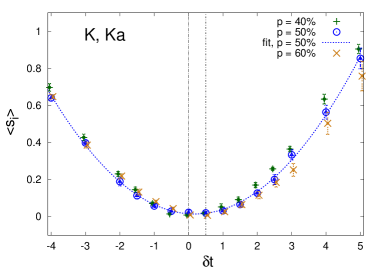
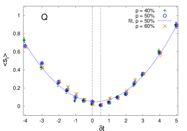
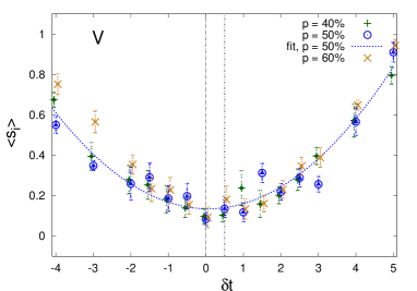
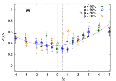
Figure 2: Mean and uncertainty of $s_{i}(\delta t)$ [cf. Eq. (18)] in the K and Ka, Q, V, and W bands, from top to bottom, respectively, as a function of $\delta t$ in units of observing intervals. For each band, symbols show the mean and standard error in the mean for the 6 or 12 DA/year combinations in that band. In addition to $s_{i}$ based on $\sigma_{i}$ defined as the median standard deviation in a map ($\odot$, labelled “$p=50\%$”), equivalent statistics based on the 40% ($+$) and 60% ($\times$) percentiles are also shown. A least-squares best-fit parabola to the 50% curve is shown in each panel for convenience, but not used in estimating the minima $\tau_{i}$. The values $\delta t=0$ and $\delta t=0.5$, favoured by Liu et al. (2010a) [version (i)] and the WMAP collaboration, respectively, are shown as vertical lines. Offsets in $\delta t$ of $\pm 0.05$ are applied to the $40\%$ and $60\%$ percentile statistics to reduce symbol overlap.

Liu et al. (2010a)’s convention for labelling the timing offset, including the sign, is retained. That is, the center parameter for determining the timing offset is generalised to an arbitrary floating point value, written here as $\delta t$, expressed as a fraction of an observing time interval in a given band. Liu et al. (2010a)’s hypothesis of what is the correct offset, interpreted to mean that the true error occurred during the calibration step and not during the mapmaking step, includes two versions, labelled (i) and (ii) above (Sect. 1). As (i) a “timing interpolation”, the hypothesis can be defined to mean $\delta t=0$ in all bands. The WMAP collaboration’s preferred timing offset corresponds to $\delta t=0.5$. The second version of Liu et al. (2010a)’s hypothesis, (ii) above (Sect. 1), is the TOD file fixed timing offset relative to the WMAP collaboration’s choice, i.e. $(\delta t-0.5)\Delta t=-25.6$ ms, where $\Delta t$ is the exposure time of a single observation in the K and Ka, Q, V, or W band, i.e. 128 ms, 102.4 ms, 76.8 ms, or 51.2 ms, respectively. Thus, in the W band, $-25.6$ ms relative to $\delta t=0.5$ corresponds to $\delta t=0$, while at lower frequencies, the offset fixed in milliseconds corresponds to values of $\delta t$ between 0 and 0.5. The different hypotheses of the timing offset are summarised in Table 1 as a function of waveband.

As explained in Sect. 2.1, the pixel sizes must be large enough to avoid introducing variance due to the incorrect inversion of small-scale signals (e.g. objects at the few-arcminute scale are blurred by $g^{-1}$). Hence, a HEALPix (Górski et al. 1999) resolution of $N_{\mathrm{side}}=8$, i.e. pixel sizes of about $7.3^{\circ}$, is adopted here. This should reduce the chance that small-scale effects contaminate the effect of interest here.

For each DA/year combination $i$ in each band, maps of the signal $\left.\left<\delta T\right>\right|_{\phi,\theta}$ and the square signal $\left.\left<(\delta T)^{2}\right>\right|_{\phi,\theta}$ are calculated over $-4\leq\delta t\leq 5$, i.e. at values symmetric around $\delta t=0.5$, with smaller intervals closer to that value. This wide range in $\delta t$ is used because, as for the blurring effect analysed in Roukema (2010), exaggerating the absolute timing offset should strengthen the effect of using a wrong value.

For a given $\delta t$, the two maps are used to infer a map of the standard deviation per pixel $\sigma_{g_{\delta t}^{-1}(\delta T)}\big{|}_{\phi,\theta}$ where $\delta T$ now represents the calibrated (whether correctly or not) TOD. Let $\sigma_{i}(\delta t)$ be the median of this quantity over the map, as in Eq. (17), where invalid pixels (mostly in the Galactic Plane) are ignored.

These “median standard deviations” $\sigma_{i}(\delta t)$ are normalised over $\delta t$ internally within each sample $i$ in order to give approximately equal weight to the different DA/year samples $i$ in a given band. That is, the minimum $A_{i}$ and maximum $B_{i}$ of $\sigma_{i}(\delta t)$ are used to calculate

$$s_{i}(\delta t):=\frac{\sigma_{i}(\delta t)-A_{i}}{B_{i}-A_{i}}.$$ (18)

In order to estimate the minimum of $s_{i}(\delta t)$ in a given DA/year combination in a given band, a smooth, symmetric function is needed. The simplest obvious choice is a parabola. Since $s_{i}$ is normalised to the range $[0,1]$, the parabola $a_{i}(\delta t)^{2}+b_{i}\delta t+c_{i}$ that least-squares best-fits $s_{i}(\delta t)$ is found, giving an estimate

$$\tau_{i}:=-b_{i}/(2a_{i})$$ (19)

of the $\delta t$ value that minimises $s_{i}(\delta t)$. For a given band, each of the 6 (K and Ka, Q, or V) or 12 (W) DA/year combinations $i$ yields an estimate $\tau_{i}$. Under the assumption of statistical independence among the DA/year combinations, the median $\mu_{1/2}(\tau_{i})$ and standard error in the median $\sigma_{\mu_{1/2}(\tau_{i})}$ give an estimate of the optimal timing offset for the inversion of a would-be timing offset during calibration of the uncalibrated TOD in that waveband.

For the purposes of testing the sensitivity to the fitting method (Sect. 4.1), additional calculations at $\delta t=-5,-2.5$ were made in order to have a sample that is symmetric around $\delta t=0$, i.e. to test sampling sensitivity, for all wavebands. Extra maps were also calculated for $\delta t=-10,\ldots,-6,6,\ldots,10$ in W to see if a wider range in $\delta t$ gives a better defined minimum (Sect. 4.2).

Table 2: Quadratic fit estimates of the timing offset [median $\mu_{1/2}(\tau_{i})$ and standard error in the median $\sigma_{\mu_{1/2}(\tau_{i})}$, Eq. (19)] that minimises the standard deviation per pixel over $\delta t$ intervals symmetric around $\delta t=0.5$ in the range $-4\leq\delta t\leq 5$, for 6 DA/year combinations $i$ in the K and Ka bands grouped together, for 6 DA/year combinations $i$ in each of the Q and V bands separately, and for 12 DA/year combinations $i$ in the W band, shown in units of an observing interval $\Delta t$, and in ms, compared to the WMAP collaboration preferred value of $\delta t=0.5$.

$$\begin{array}[]{c rr r rr }\hline\cr\rule[-6.45831pt]{0.0pt}{19.37494pt}&\mu_{1/2}(\tau_{i})&\sigma_{\mu_{1/2}(\tau_{i})}&\Delta t&\mu_{1/2}(\tau_{i}-0.5)\Delta t&\sigma_{\mu_{1/2}(\tau_{i})}\Delta t\\ \mathrm{units:}&\Delta t&\Delta t&\mathrm{ms}&\mathrm{ms}&\mathrm{ms}\\ \mathrm{band}\\ \hline\cr\rule[-6.45831pt]{0.0pt}{19.37494pt}\mbox{K, Ka}&0.20&0.06&128.0&-38.4&8.3\\ \mathrm{Q}&0.24&0.03&104.2&-27.1&2.8\\ \mathrm{V}&-0.06&0.11&76.8&-43.0&8.1\\ \mathrm{W}^{{}^{\mathrm{a}}}&-0.41&3.74&52.1&-47.4&194.8\\ \hline\cr\rule[-6.45831pt]{0.0pt}{19.37494pt}\mathrm{all}^{{}^{\mathrm{b}}}&0.22&0.02&-&-29.7&2.5\\ \hline\cr\end{array}$$

^aIn W, the best-fit parabola for one of the year/DA combinations had a maximum and was ignored.
^bMean and standard error, weighted by the standard error, calculated either in observing interval units (ignoring the dependence of $\Delta t$ on waveband), or in ms compared to $\delta t=0.5$.

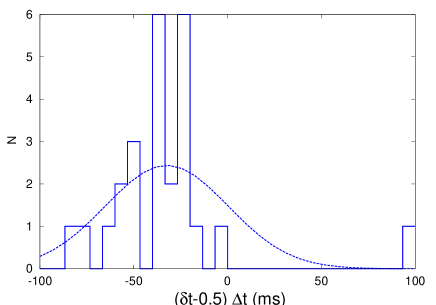
Figure 3: Histogram of the timing offset estimates $\mu_{1/2}(\tau_{i}-0.5)\Delta t$ from the individual DA/year combinations, of which per-band statistics are listed in Table 2, and a Gaussian distribution appropriately normalised.

3 Results

Calculations on 4-core, 2.4 GHz, 64-bit processors with 4 Gib RAM, using GDL-0.9$\sim$rc4 running under GNU/Linux, took about 2–6 hours per map, depending on waveband. Figure 2 clearly shows that the per pixel variance of the maps is minimised near the preferred time offsets of the WMAP collaboration and Liu et al. (2010a). Time offsets of several observing intervals above or below these values clearly increase the per pixel variance. It is not clear in the figure whether any of the claimed offset hypotheses is significantly preferred as a sharp minimum. However, the approximate symmetry axes of the function shapes clearly lie at lower $\delta t$ than the central value $\delta t=0.5$.

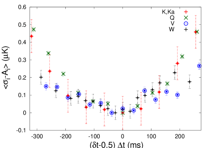
Figure 4: Median standard deviation in $\mu$K with zeropoints removed, i.e. $\sigma_{i}(\delta t)-A_{i}$ as in Eq. (18), averaged (mean) over DA/year combinations in each of the K and Ka, Q, V, and W bands (symbols as indicated in the figure), as a function of timing offset in ms relative to the WMAP collaboration hypothesis, i.e. $(\delta t-0.5)\Delta t$. Error bars are standard errors in the mean. The timing offset range is centred on that of the hypothesis favoured from Table 2, i.e. $(\delta t-0.5)\Delta t=-25.6$.

Table 2 shows the statistics of $\tau_{i}$, the minimum of $s_{i}$ for the individual DA/year combination for each waveband. Comparison with Table 1 shows that the WMAP collaboration’s preferred timing offset is rejected to high significance in the lower frequency bands, i.e. 4.5$\sigma$ (K, Ka), $8.2\sigma$ (Q), and $5.2\sigma$ (V), and not constrained in the W band. Moreover, the K and Ka bands, and the Q band, also reject version (i) of Liu et al. (2010a)’s hypothesis to high significance, i.e. $3.0\sigma$ (K, Ka) and $7.6\sigma$ (Q). Hence, both the WMAP collaboration’s preferred timing offset and version (i) of Liu et al. (2010a)’s hypothesis are rejected to high significance by minimisation of per pixel variance of maps made from the calibrated, filtered TOD.

In contrast, the final two numerical columns in Table 2 show that version (ii) of Liu et al. (2010a)’s timing offset, defined as the TOD file timing offset of $-25.6$ ms, is consistent with all wavebands, at $1.5\sigma,0.5\sigma,2.1\sigma,$ and $0.1\sigma$ in K and Ka, Q, V, and W, respectively. The weighted mean $\mu_{1/2}(\tau_{i}-0.5)\Delta t=-29.7\pm 2.5$ ms rejects the WMAP collaboration’s hypothesis at $11.9\sigma$ and agrees with the fixed TOD file timing offset hypothesis at $1.6\sigma$.

The above significance estimates assume that the statistic $\tau$ is normally distributed. Figure 3 shows the 25 timing offset estimates, from individual 30 DA/year combinations, that lie in the range $(-100,100)$ ms. The distribution is not well-modelled by a Gaussian distribution. A Kolmogorov-Smirnov test with the mean and standard deviation of the data rejects the hypothesis that the distribution is Gaussian with $p=1.4\%$. Could this affect the significance in rejecting the $\delta t=0.5$ hypothesis?

It is clear that it would be difficult to reconcile the distribution in Fig. 3 with having a median of 0 ms, especially given that the distribution is sampled many times. This can be tested more formally. To non-parametrically test the hypothesis that the median of the distribution is 0 ms, $10^{6}$ bootstrap resamples from the distribution were made. These give a 99.999% confidence interval for the median of the distribution to be $\mu_{1/2}(\tau_{i}-0.5)\Delta t\in(-54,-20)$ ms. Thus, the WMAP $\delta t=0.5$ hypothesis can be conservatively rejected at $99.999\%$ confidence. The same non-parametric method gives the $(2.5\%,97.5\%)$ confidence interval to be $(-47,-26)$ ms, i.e. taking into account Bennett et al. (2003a)’s (Sect. 6.1.2) estimate of the uncertainty in the timing as 1.7 ms, the hypothesis of a $-25.6$ ms offset is consistent with the data.

3.1 Quadrupole overestimation induced by the calibration error

Unfortunately, the simple procedure presented here is only sufficient to provide evidence for the timing-offset–induced calibration error, not for compiling improved maps directly from the calibrated TOD. As explained in Sect. 2.1, a timing-offset–induced calibration error on a signal dominated by the dipole can be approximately reversed, since the calibration is itself based on a model dipole that is a good approximation to the measured dipole. However, the remaining signal is not a dipole, so it is more difficult to correct the remaining components of the wrongly-calibrated signal. As shown in Roukema (2010), the present method of reversing the calibration error, i.e. the use of $g^{-1}$, introduces a blurring effect on small ($\sim 4{{}^{\prime}}$) scales. To obtain CMB sky maps with the calibration error fully removed, it is not obvious that there is a simpler alternative to redoing the full calibration of the uncalibrated TOD.

Nevertheless, an approximate reversal of the $-25.6$ ms timing-offset–induced calibration error in at least the dipole component of the signal is possible using the same data analysis pipeline as above. In this case, by how much does the quadrupole decrease when the artificial quadrupole-like signal is approximately removed?

Using the presently available version of the WMAP 3-year, calibrated, filtered TOD in the W band, i.e. the band where the cosmological signal is the least affected by foregrounds, the quadrupole can be calculated consistently for maps at both $\delta t=0.5$, the incorrect timing offset, and $\delta t=0$, the timing offset that yields approximately corrected maps. Using maps made at a resolution of $N_{\mathrm{side}}=512$, and subtracting the 3-year maximum entropy synchrotron, free-free and dust maps provided by the WMAP collaboration, pseudo-$C_{l}$ estimates (after monopole and dipole removal) from the 3 years, for the 4 W band DA’s, are $(3/\pi)C_{2}=170\pm 4\,\mu$K² and $103\pm 4\,\mu$K², for $\delta t=0.5$ and $\delta t=0$, respectively, for the KQ85 sky mask, and $(3/\pi)C_{2}=79\pm 3\,\mu$K² and $41\pm 2\,\mu$K² for the KQ75 sky mask, where errors are standard errors in the mean over the 12 DA/year combinations, and 80 map iterations are made for each DA/year combination. The dipole removal has little effect on these estimates. Removal of only the monopole gives $(3/\pi)C_{2}=170\pm 4\,\mu$K² and $103\pm 4\,\mu$K², for $\delta t=0.5$ and $\delta t=0$, respectively, for the KQ85 sky mask, and $(3/\pi)C_{2}=78\pm 3\,\mu$K² and $40\pm 2\,\mu$K² for the KQ75 sky mask. Hence, the $-25.6$ ms timing-offset–induced calibration error implies that estimates of the CMB quadrupole amplitude $(3/\pi)C_{2}$ based on WMAP 3-year W band sky maps derived from the incorrectly calibrated TOD are overestimated by $64\pm 6\%$ and $94\pm 10\%$ for the KQ85 and KQ75 sky masks, respectively (for removal of both the monopole and dipole).

This is a significant and substantial systematic error. Given the differences in method and data subsets [e.g., Liu & Li (2010a) estimate cross-quadrupoles of the V and W five-year data, while the present estimate is the W 3-year auto-quadrupole], the KQ75 drop in quadrupole power appears to be roughly consistent with that of Sect. 5.3 of Liu & Li (2010a), i.e. greater than that of Moss et al. (2010)’s toy model estimate (Fig. 1 caption). Moreover, the problem of large-scale CMB power being concentrated towards the Galactic Plane is exacerbated with this approximate correction of the calibration error. The Galactic Plane is the part of the sky where difficult-to-estimate systematic error can most be suspected.

Table 3: Quadratic fit estimates [median $\mu_{1/2}(\tau_{i}-0.5)\Delta t$ and and standard error in the median, in ms] of minimum standard deviation, as for Table 2, using $\delta t$ intervals symmetric around $\delta t=0.0$ in the range $-5\leq\delta t\leq 5$, i.e. possibly showing bias against $\delta t=0.5$.

$$\begin{array}[]{c rr r rr }\hline\cr\rule[-6.45831pt]{0.0pt}{19.37494pt}&\mu_{1/2}(\tau_{i})&\sigma_{\mu_{1/2}(\tau_{i})}&\Delta t&\mu_{1/2}(\tau_{i}-0.5)\Delta t&\sigma_{\mu_{1/2}(\tau_{i})}\Delta t\\ \mathrm{units:}&\Delta t&\Delta t&\mathrm{ms}&\mathrm{ms}&\mathrm{ms}\\ \mathrm{band}\\ \hline\cr\rule[-6.45831pt]{0.0pt}{19.37494pt}\mbox{K, Ka}&0.20&0.07&128.0&-37.9&9.2\\ \mathrm{Q}&0.21&0.04&104.2&-30.3&3.7\\ \mathrm{V}&0.15&0.13&76.8&-26.7&9.8\\ \mathrm{W}^{{}^{\mathrm{a}}}&-0.17&11.56&52.1&-35.0&602.3\\ \hline\cr\rule[-6.45831pt]{0.0pt}{19.37494pt}\mathrm{all}&0.21&0.03&-&-30.8&3.2\\ \hline\cr\end{array}$$

^aIn W, the best-fit parabola for one of the year/DA combinations had a maximum and was ignored.

4 Discussion

4.1 Sensitivity to fitting method

These results do not appear to be sensitive to the choice of symmetrical fitting function. Least-squares hyperbolic best fits, i.e. best-fits of $a_{i}(\delta t)^{2}+b_{i}\delta t+c_{i}$ to $[s_{i}(\delta t)+0.5]^{2}$, where the vertical offset of 0.5 and positive square root of the best fit give a top quadrant hyperbola, yield similar values to those in Table 2. For example, over all wavebands, this hyperbolic fit gives $\mu_{1/2}(\tau_{i})=0.22\pm 0.04$ and $\mu_{1/2}(\tau_{i}-0.5)\Delta t=-29.4\pm 4.3$ ms.

Since the $\delta t$ values used in sampling are symmetric around $\delta t=0.5$, it is difficult to see how this could induce a bias against the $\delta t=0.5$ hypothesis. Could it lead to an inaccurate estimate in the case that $(\tau_{i}-0.5)\Delta t=-25.6$ ms is correct? Table 3 shows that using a $\delta t$ sample symmetric around $\delta t=0$ gives results compatible with those in Table 2.

Could the dependence of $s_{i}$ on $\delta t$ be asymmetric? The toy model (Sect. 2.2) does not suggest any obvious asymmetry, and it is not obvious what detailed differences between the toy model and the real data could be sufficiently asymmetric to perturb the method. Moreover, the WMAP scan paths are curved (non-geodesic) paths on the 2-sphere that have many symmetries. Nevertheless, it is not obvious that $s_{i}$ should vary with an exact symmetry around its minimum, even if approximate symmetry seems reasonable. If the dependence of $s_{i}$ on $\delta t$ approached linearity for large $|\delta t|$, then one way of testing this could be to make linear fits to subsets of data for large $|\delta t|$. However, comparison of parabolic and hyperbolic fits favours the former, i.e. $s_{i}(\delta t)$ does not appear to approach linearity for large $|\delta t|$. Thus, linear fits for large $|\delta t|$ would depend strongly on the $\delta t$ domains chosen. If an asymmetric model for $s_{i}$ dependence on $\delta t$ could be found that is close enough to parabolic in shape in order to provide fits in K and Ka, Q, and V as good as those shown in Fig. 2, then it could conceivably be possible that the $\delta t=0.5$ hypothesis could be made consistent with the resulting minima. However, in that case, the fact that the symmetry assumption gives a solution consistent with the timing offset recorded in the TOD files would have to be attributed to coincidence.

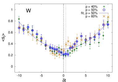
Figure 5: Mean and uncertainty of $s_{i}(\delta t)$ in the W band including a posteriori extra maps for large values of $|\delta t|$, as for Fig. 2.

4.2 Consistency between wavebands

In Fig. 2, the median standard deviation $s_{i}$ is most noisy in the W band and a little noisy in the V band. The quantitative best fit minima shown in Table 2 significantly favour the $-25.6$ ms offset hypothesis and reject the other hypotheses. The choice of intervals for mapmaking was optimised for testing the $\delta t=0$ and $\delta t=0.5$ hypotheses rather than an offset in ms, which is why the spreads of $\delta t\delta T$ for V and W are less than for K, Ka and Q. Thus, with hindsight, given the results found here, a possible explanation for the higher noisiness in V and W would be that calculations were not spread over a wide enough interval in $\delta t$ in these bands.

Another consistency check between results in different wavebands is that if the increase in $s_{i}$ away from a preferred timing offset is mainly an effect of incorrect dipole-based calibration of the observed dipole signal, then this dependence should only be weakly dependent on waveband.

Figure 4 shows the same information as in Fig. 2, with zeropoint removal but no scaling of the standard deviations, i.e. $\sigma_{i}-A_{i}$, against timing offsets in milliseconds centred on the hypothesis preferred by the data, i.e. $(\delta t-0.5)\Delta t=-25.6$ ms. In the range of approximately $(\delta t-0.5)\Delta t\in(-25.6\pm 175)$ ms, the V and W band results appear fully consistent with the K and Ka, and Q results. The V and W bands do not appear to be more noisy than the K and Ka, and Q bands. Moreover, the dependence of the effect on $(\delta t-0.5)\Delta t$ appears to be approximately independent of waveband, at least in this central range. A posteriori calculation of maps in W for larger absolute values of $\delta t$ (e.g. to about $\pm 640$ ms as in the K and Ka bands) could reasonably be expected to lead to a smaller uncertainty in this band.

Table 4: Quadratic fit estimates for usage of the calibrated TOD with an extra term, i.e. using the 80-th map iteration, as for Table 2, for the bands with shorter calculation times.

$$\begin{array}[]{c rr r rr }\hline\cr\rule[-6.45831pt]{0.0pt}{19.37494pt}&\mu_{1/2}(\tau_{i})&\sigma_{\mu_{1/2}(\tau_{i})}&\Delta t&\mu_{1/2}(\tau_{i}-0.5)\Delta t&\sigma_{\mu_{1/2}(\tau_{i})}\Delta t\\ \mathrm{units:}&\Delta t&\Delta t&\mathrm{ms}&\mathrm{ms}&\mathrm{ms}\\ \mathrm{band}\\ \hline\cr\rule[-6.45831pt]{0.0pt}{19.37494pt}\mbox{K, Ka}&0.32&0.06&128.0&-23.3&7.3\\ \mathrm{Q}&0.40&0.13&104.2&-10.0&13.7\\ \mathrm{V}&0.11&0.65&76.8&-30.3&49.7\\ \hline\cr\rule[-6.45831pt]{0.0pt}{19.37494pt}\mathrm{all}&0.33&0.05&-&-20.5&6.4\\ \hline\cr\end{array}$$

This is indeed the case. Extra maps were calculated for $\delta t=-10,\ldots,-6,6,\ldots,10$ in the twelve W band DA/year combinations. If all the W maps are analysed together, the resulting best estimates are $\mu_{1/2}(\tau_{i})=0.19\pm 2.24$ and $\mu_{1/2}(\tau_{i}-0.5)\Delta t=-16.1\pm 116.8$ ms. However, Fig. 5 shows that the dependence of $s_{i}$ on $\delta t$ in the W band is more complex than the quadratic dependence that gives visually acceptable fits in the K and Ka, Q, and V bands.

Figure 4 also shows that beyond the central range where the different bands appear consistent, there appear to be significant differences in the amplitude of the variation in $s_{i}$ between the different wavebands, given the uncertainties estimated among DA/year combinations within each waveband, even though the estimates of minima are clearly consistent (Table 2). This variation among wavebands might be due to an increased role of non-dipole components of the signal, e.g. Galactic foregrounds that are brightest in the lower frequencies. Since cosmological perturbations should be much weaker than both the dipole and low frequency foregrounds, the approximate frequency independence of the effect near the minimum variance and frequency dependence away from the minimum is qualitatively consistent with the effect near the minimum being dominated by the dipole, and the effect further from the minimum involving coupling effects between the dipole calibration, the measured dipole, and foregrounds. The beam size and sidelobe effects reported by Sawangwit & Shanks (2010) and Liu & Li (2010b) may be related to this latter speculation.

4.3 Sidelobe and other beam effects

Sawangwit & Shanks (2010) have estimated that WMAP beam profiles at faint flux density levels, especially in the W band and weakly in the V band, are wider than those estimated by the WMAP collaboration for bright flux density levels. Liu & Li (2010b) have suggested that WMAP sidelobe interactions with the dipole signal create an effect that may be effectively modelled as if it were a positional offset. From Fig. 1 of Page et al. (2003) and Fig. 2 of Hill et al. (2009), for the first year and 5-year WMAP data releases respectively, it is clear that sidelobes in the beam shapes are strong for the W DA’s, weak for the V DA’s, and much weaker for the K, Ka, and Q DA’s.

The beam shape dependence on waveband suggests an explanation not only for the variation in $s_{i}$ dependence on $(\delta t-0.5)\Delta t$ among wavebands at large $|(\delta t-0.5)\Delta t|$, but also for the complexity in the shape of $s_{i}(\delta t)$ in the W band (Fig. 5) and the associated large uncertainty in $\mu_{1/2}(\tau_{i}-0.5)\Delta t$ in the W band (Table 2). The (partial) invertibility of a timing-offset–induced calibration as presented in this work depends on the details of the scanning pattern. For a complicated beam profile, the relation between the sidelobe orientation, the scanning pattern, and a slightly displaced dipole, is likely to be complicated. For a simple profile, the relation is likely to be simpler, i.e. less noisy. Thus, the complexity in $s_{i}(\delta t)$ in the W band is qualitatively consistent with Liu & Li (2010b)’s estimate that sidelobe interaction with the dipole is important in mapmaking, given the WMAP collaboration’s estimates of the beam profiles shown in Fig. 1 of Page et al. (2003) and Fig. 2 of Hill et al. (2009). It is also qualitatively consistent with the result of Sawangwit & Shanks (2010) that the difference between their radio-source–based beam profile estimates and the WMAP collaboration’s Jupiter-based estimates is strongest in the W band.

4.4 Extra term from iterated maps

Although use of an iterated map is equivalent to adding an extra term to Eqs (13) and (14), introducing more noise into the method, the result should be statistically compatible with the above results. Checking the bands with fewer numbers of DA’s and observations, i.e. adding the 80-th map iteration to these equations, took about a calendar month of calculations. The results are shown in Table 4. These mainly consist of an increase in the noise, with a slight increase in $\delta t$ values, i.e. $\mu_{1/2}(\tau_{i}-0.5)\Delta t=-20\pm 6$ ms. This estimate still disagrees with $\delta t=0$ to high significance, and agrees with $(\delta t-0.5)\Delta t=-25.6$ ms at $0.8\sigma$.

4.5 Devil’s advocate: could the calibration be correct?

It is difficult to see how the variance per pixel can be decreased by an arbitrary shuffling of the TOD. The simplest explanation for the best estimate of $\mu_{1/2}(\tau_{i}-0.5)\Delta t=-29.7\pm 2.5$ ms is that the $-25.6$ ms timing offset correction was not implemented when the WMAP uncalibrated TOD were calibrated. However, could it be possible to avoid this inference, i.e. could the calibration be correct? Some possibilities and counterarguments are as follows.

• As mentioned above, a model in which the dependence of $s_{i}$ on $\delta t$ is asymmetric might, in principle, give the minimum variance per pixel to occur near $\tau_{i}=0.5$. This would require a heuristic model for the asymmetric behaviour, and at least qualitatively would seem to require a much more complex shape than a parabola.

  • In this case, it would be a coincidence that the symmetry assumption gives a result consistent with one of the two versions of Liu et al. (2010a)’s hypothesis, as listed in Table 1. That is, the successful prediction of one of the two versions of Liu et al. (2010a)’s hypothesis would be a coincidence.

• A heuristic model could relate to the fact that the K, Ka, and Q bands have much stronger Galactic contamination than the V (and W) bands. Could the $\mu_{1/2}(\tau_{i}-0.5)\Delta t=-29.7\pm 2.5$ ms estimate be primarily an effect of Galactic contamination?

  • The dependence of Galactic contamination on waveband is very strong going from K to W. Tables 2 and Table 3 do not show any obvious trend in this sense.

  • The statistic $s_{i}$ is a normalisation of $\sigma_{i}$, which is the median, over the pixels of a given map, of the standard deviation per pixel. For Galactic contamination to affect the median, by shifting flux density onto or off given pixels, it would need to affect about half of the pixels at high Galactic latitude. However, a $-25.6$ ms timing offset corresponds to only 4^′, while pixel sizes are about 7.3^∘, i.e. about four orders of magnitude greater in solid angle. Even in the K and Ka bands, where the Galactic contamination is very strong, the number of tiny positional shifts of flux density onto or off a given pixel should be very high, so that the median over all valid pixels could be expected to vary smoothly and symmetrically around the correct timing offset.

  • The coincidence argument also applies here. The Galactic contamination would have to mimic one of the two versions of Liu et al. (2010a)’s hypothesis by chance, in sign ($\tau_{i}<0$), in amplitude, and in having an approximately constant value expressed as $\mu_{1/2}(\tau_{i}-0.5)\Delta t$.

• Could the small-scale blurring effect (Roukema 2010, and references therein) have played a significant role in this analysis?

  • If it did, then it would have caused the results to be biased in favour of $\tau_{i}=0.5$, i.e. $\mu_{1/2}(\tau_{i}-0.5)\Delta t=0$ ms. In other words, correcting the present result for the small-scale blurring effect would shift it in the opposite direction, giving $\mu_{1/2}(\tau_{i}-0.5)\Delta t<-29.7\pm 2.5$ ms. This would worsen the rejection of the $\tau_{i}=0.5$ hypothesis.

• Liu & Li (2010a) showed and Moss et al. (2010) confirmed that the CMB quadrupole is reduced in amplitude for $\Delta t(\delta t-0.5)\sim-25.6$ ms. If this is just a coincidence that relates the CMB quadrupole, the velocity dipole and the WMAP spacecraft scan pattern, could the variance minimisation method be strongly biased towards minimisation of the quadrupole, so that these constitute two instances of a single coincidence? For example, let us suppose that $\delta t=0.5$ is the correct value. It is already known that in this case, the mean signal at $\delta t=0$ will be smaller. Could this imply that the standard deviation per pixel at $\delta t=0$ would be smaller too?

  • If $\delta t=0.5$ were really correct, then, although the mean signal at $\delta t=0$ will be smaller, this would only be a result of the fortuitous cancelling, in the mean, of a component of the real signal by the dipole-induced difference signal. However, reducing the mean by the addition of anticorrelated errors does not reduce the standard deviation per pixel. The scatter induced by a wrong assumed value of $\delta t$ is not cancelled by a reduced mean value.

  • Calibration errors induced by a wrong value of $\delta t$ apply to the full CMB signal, not just to the quadrupole part of the signal. The latter is a very weak part of the full CMB signal. Thus, scatter induced by a wrong value of $\delta t$ can have only a weak dependence on the quadrupole. Table 2 shows that $\delta t=0.5$ is still strongly rejected in the K and Ka, and Q bands, where galactic foregrounds play a strong role.

Retaining the hypothesis that the calibration was correct does not seem to be easy.

5 Conclusion

While the $-25.6$ ms offset between the times in the Meta Data Set and the Science Data Set in the WMAP TOD files, discovered by Liu et al. (2010a), did not lead to an error in compiling the calibrated, filtered, 3-year TOD into maps (Roukema 2010), it is difficult to avoid the conclusion that this timing offset did induce an error at the calibration step. The two different versions of Liu et al. (2010a)’s hypothesis gave numerical predictions, listed in Table 1. The constant offset in ms hypothesis is consistent with the analysis of the variance maps, summarised in Table 2. This result does not seem to be sensitive to the fitting method (Sect. 4.1), it is consistent among all wavebands (Sect. 4.2), using highly iterated maps adds noise and gives consistent results (Sect. 4.4), and alternative explanations seem to be speculative and/or fail to save the $\delta t=0.5$ hypothesis (Sect. 4.5). The timing offset that is numerically implicit in the TOD files (e.g., see Appendix A, Roukema 2010) would appear to provide the simplest explanation. A new analysis of 7 years of Q, V, and W band WMAP TOD by Liu et al. (2010b) finds a similar result. Thus, it appears that (1) in the calibration step, both the spacecraft attitude quaternion timestamps and the observational timestamps were used, for the dipole and observational data, respectively, inducing a calibration error, while (2) in the mapmaking step, the observational timestamps were (correctly) assumed to be correct both for dipole and observational data, inducing no further error, but retaining the original calibration error. This supports the claims by Liu et al. (Liu & Li 2010a; Liu et al. 2010a) that the CMB quadrupole has been substantially overestimated. A rough estimate made here is that the quadrupole estimated in maps based on the wrongly calibrated TOD is overestimated by about $64\pm 6\%$ to $94\pm 10\%$ for the KQ85 and KQ75 sky masks respectively (Sect. 3.1).