ROM2F/2010/11

Dynamical Supersymmetry Breaking in Intersecting Brane Models
F.Fucito, A. Lionetto, J. F. Morales, and R. Richter
I.N.F.N. Sezione di Roma Tor Vergata

and

Dipartimento di Fisica, Universitá di Roma “Tor Vergata”
Via della Ricerca Scientifica, 00133 Roma, Italy

Abstract

In this paper we study dynamical supersymmetry breaking in absence of gravity with the matter content of the minimal supersymmetric standard model. The hidden sector of the theory is a strongly coupled gauge theory, realized in terms of microscopic variables which condensate to form mesons. The supersymmetry breaking scalar potential combines F, D terms with instanton generated interactions in the Higgs-mesons sector. We show that for a large region in parameter space the vacuum breaks in addition to supersymmetry also electroweak gauge symmetry. We furthermore present local D-brane configurations that realize these supersymmetry breaking patterns.

1 Introduction

Breaking supersymmetry (SUSY) has always proved to be a challenging and daunted task. Of all the possible options, dynamical SUSY breaking (DSB) remains one of the most exciting and economical choices of breaking SUSY. In this framework, SUSY is a symmetry of the effective action and it is broken spontaneously by the choice of the field theory vacuum. As it is well known, the original toy models, in which SUSY was broken by giving a vacuum expectation value (vev) to the F or D-terms, gave a sparticle spectrum at odds with observations. This is why in the usual SUSY extensions of the Standard Model (MSSM), the breaking is achieved via the introduction of suitable terms in the Lagrangian called soft SUSY breaking terms. They do not spoil the divergence properties of the theory and also participate to the mechanism for the gauge symmetry breaking of the theory. SUSY breaking is thus intimately connected with all the main features of the MSSM. The common lore wants soft SUSY breaking terms to be generated at higher energies with respect to the mass of the sparticles in a so called hidden sector. SUSY breaking is then communicated to the visible sector via (gauge or gravity) messenger particles. Recently many good books on SUSY have appeared in which these issues are considered at length [1, 2, 3, 4, 5, 6].

The progress in the computation of non perturbative effects in gauge and SUSY theories, has opened up a new possibility for SUSY breaking: the classical potential has a trivial vacuum which is corrected by quantum effects. The quantum potential then exhibits DSB. Already at the level of SUSY gauge theories, the existence of condensates, driven by non perturbative effects, does not immediately translates into SUSY breaking. Each case must be carefully examined: the standard criterion is to look for a global symmetry, spontaneously broken, in a theory which has no flat directions. Another standard strategy is to look for inconsistencies in the theory i.e. for a clash between two different conditions which have to be simultaneously satisfied in order to preserve SUSY (for example existence of a condensate which then violates the Konishi anomaly) [7, 8, 9, 10]. These results were first obtained for non chiral QCD like theories. Their extension to chiral models of SUSY GUT type was discussed in [9] and in the framework of gauge mediation in [11, 12, 13].

How to incorporate all of this into the framework of string theory is then a completely different problem. Recently some of the authors of the present paper [14] have analysed a quiver model realizing a dynamical SUSY breaking scenario for a GUT theory. In this paper we want to take a further step and consider string intersecting models with the matter content of the MSSM. There has been much work recently to embed the SM and MSSM using intersecting branes:. here we discuss SUSY breaking in this scenario. Therefore we consider a model where SUSY is broken spontaneously via a non-perturbatively generated superpotential in a hidden strongly coupled gauge theory. The non-perturbative superpotential will induce spontaneous breaking of gauge and SUSY via an articulate conspiracy of gauge (D-terms) and Yukawa (F-terms) interactions. Some of the steps we will take resemble the so called KKLT approach followed in [20] to stabilize some of the moduli of a string theory compactification and more recently in [21, 22, 23]. However in our case gravity plays no role: we just focus on the open string sector. We thus postulate that the details of the compactification are already taken care of, that moduli have been (completely or partially) stabilized and that the closed string dynamics is not affecting our results. As we will see, these positions are not oversimplifying our model. The open string sector must obey tight constraints to be consistent, regardless of the closed strings.

This is the plan of the paper: in Sections 2 and 3 we will discuss our model from the point of view of field theory. In Sections 4 and 5 we will discuss local D-brane configurations which, at low energy, lead to the field theories of the previous Sections.

2 Susy-breaking extensions of the MSSM

In this work we present two extensions of the MSSM which naturally give rise to SUSY and electroweak gauge symmetry breaking. In both cases the interplay of F and D-terms is crucial for the SUSY and electroweak gauge symmetry breaking. As we will see later in Section 5 such extensions of the MSSM can naturally arise from D-brane compactifications.

Let us start by stating the gauge symmetry of the setups

$$SU(3)_{C}\times SU(2)_{L}\times U(1)_{Y}\times U(1)\times SU(3)_{H}\,\,,$$ (1)

which in addition to the usual SM gauge symmetry contains an abelian gauge symmetry and a strongly coupled hidden $SU(3)_{H}$.

The chiral matter sector contains the usual MSSM matter content, namely the quarks and leptons

$$\vec{\Phi}=\{Q_{L},L,u^{c},d^{c},e^{c},\nu^{c}\}\,\,,$$ (2)

which are collected in the vector $\vec{\Phi}$, where capital letters refer to left-handed superfields, while lower case letters denote right-handed fields. In addition to the MSSM particles we have the Higgs fields $H_{u,d}$ and two quark anti-quark pairs $Q_{i}$ and $\widetilde{Q}_{i}$ , $i=1,2$, charged with respect to the hidden $SU(3)_{H}$ and the additional $U(1)$. Moreover, depending on the considered setup there may be an additional field $Y$, which is neutral under the SM gauge groups and only charged under the $U(1)$.

The hidden $SU(3)_{H}$ gauge theory with two quark anti-quark pairs $Q$ and $\widetilde{Q}$ will condensate via the generation of a Affleck, Dine and Seiberg superpotential

$$W_{\rm non-pert}=\frac{\Lambda^{7}}{{\rm det}\,(M_{ij})}\,\,,$$ (3)

where $M_{ij}=Q_{i}\widetilde{Q}_{j}$ is the meson matrix. At the scale $\Lambda$ the gauge theory is effectively described in terms of the mesons and baryons of $SU(3)_{H}$ which can be taken as the microscopic degrees of freedom of the low energy physics. In the following we will denote by $\Lambda M_{i}$, the eigenvalues of the meson matrix $M_{ij}$ and will work with the $M_{i}$ as fundamental degrees of freedom. Thus the SUSY - electroweak gauge symmetry breaking matter content, the Higgs-meson sector, is given by

$$\vec{X}=\{H_{u},H_{d},M_{i},Y\}\,\,,$$ (4)

where the presence of $Y$ depends on the choice of the specific setup.

As we will see later in Section 5 in D-brane compactifications the hypercharge is a linear combination of various $U(1)$’s. Explicitly

$$U(1)_{Y}=\frac{1}{2}U(1)_{d}+\frac{1}{2}U(1)_{e}+...\qquad U(1)=\frac{1}{2}U(1)_{e}-\frac{1}{2}U(1)_{d}\,\,,$$ (5)

where the dots indicate that there are further contributions for the hypercharge from other $U(1)$’s under which the Higgs-meson fields are uncharged. For later convenience we label each $U(1)$ by a subscript that will later specify its D-brane origin.

Below in Table 1 we display the non-trivial charges of the fields $\vec{X}$ in the Higgs-meson sector with respect to the $SU(2)$ electroweak and $U(1)_{d,e}$ symmetries.

	$H_{u}$	$H_{d}$	$M_{1}$	$M_{2}$	Y
$SU(2)$	${\bf 2}$	${\bf 2}$	${\bf 1}$	${\bf 1}$	${\bf 1}$
$U(1)_{d}$	$0$	$-1$	$1$	$-1$	$1$
$U(1)_{e}$	$1$	$0$	$-1$	$1$	$-1$

Table 1: $SU(2)\times U(1)_{d}\times U(1)_{e}$-charges of the Higgs-meson sector

With that choice of charges the generic superpotential containing only the fields $\vec{X}$ and respecting the abelian symmetries $U(1)_{d}$ and $U(1)_{e}$ is of the form

$$W=\mu H_{u}H_{d}M_{1}+mM_{2}M_{1}+\frac{\Lambda^{5}}{M_{1}M_{2}}+\Big{(}\mu_{Y}H_{u}H_{d}Y+m_{Y}M_{2}Y\Big{)}\,\,.$$ (6)

In absence of the field $Y$, clearly the last two terms of (6) are absent.

In order to ensure that the color and electromagnetic gauge symmetries remain unbroken, we require the vanishing of all the vev’s of the MSSM matter fields $\vec{\Phi}$. We look then for solutions with

$$\langle\vec{\Phi}\rangle=0\qquad\langle\vec{X}\rangle=x+\theta^{2}F_{x}$$ (7)

In the following we will try to find SUSY and electroweak gauge symmetry breaking minima satisfying (7). Thus we extremize the scalar potential only with respect to the fields $\vec{X}$. We will show in Section 3 that for a wide range in parameter space, SUSY and the electroweak gauge symmetries are broken in the $\vec{X}$ sector.

2.1 The Lagrangian

After discussing the general setup above let us now describe in more details the Lagrangians of the models we will consider. For simplicity we take a canonical Kähler potential for the Higgs-meson fields $\vec{X}$. More precisely we take the Kähler potential to be

$$K(\vec{X},\vec{X}^{\dagger},\vec{\Phi},\vec{\Phi}^{\dagger})=\vec{X}\vec{X}^{\dagger}+k_{ij}(\vec{X},\vec{X}^{\dagger})\Phi_{i}\Phi_{j}^{\dagger}+...\,\,\,\,.$$ (8)

Thus the Kähler metric for the scalar fields $\vec{X}$ will take a canonical form after taking into account the vanishing vev’s of the MSSM matter fields $\vec{\Phi}$. We allow for a general $\vec{X}$-dependence of the functions $k_{ij}$ specifying the Kähler metric for the matter fields $\vec{\Phi}$. When SUSY is broken $F_{X}\neq 0$, these Kähler interactions provide soft symmetry breaking mass terms (of order $k_{ij}^{\prime\prime}|F_{X}|^{2}$) for sparticles. These functions should then satisfy the phenomenological requirement that the masses of sparticles are beyond the observable limits. Let us stress though that the specific type of Kähler potential does not affect our conclusions regarding SUSY and gauge symmetry breaking. A similar $\vec{X}$-dependence can be introduced in the gauge kinetic functions $\tau_{a}(\vec{X})$ in order to induce soft symmetry breaking masses (of order $\tau_{a}^{\prime}F_{X}$) for the gauginos of the unbroken symmetries $SU(3)_{C}\times U(1)_{\rm em}$ of the MSSM .

With these assumptions the Lagrangians leading to the D and F terms can be written as

$$\mathcal{L}_{\rm D}=\left(k_{ij}(\vec{X},\vec{X}^{\dagger})\,\Phi_{i}^{\dagger}e^{V}\Phi_{j}+\vec{X}^{\dagger}e^{V}\vec{X}+\xi_{a}V_{a}\right)\Big{|}_{\theta^{2}\bar{\theta}^{2}}+{\rm h.c.}$$

$$\mathcal{L}_{F}=\left[\tau_{a}(\vec{X})\textnormal{Tr}(W^{(a)}W^{(a)})+W(\vec{X},\vec{\Phi})\right]\Big{|}_{\theta^{2}}+{\rm h.c.}\,\,.$$ (9)

with $k_{ij}(\vec{X},\vec{X}^{\dagger})$, $\tau_{a}(\vec{X})$ the quark and lepton Kähler function and $W(\vec{X},\vec{\Phi})$ the superpotential. We will split the latter into two terms according to the number of quark and lepton superfields involved

$$W(\vec{X},\vec{\Phi})=W_{0}(\vec{X})+W_{2}(\vec{X},\vec{\Phi})\,\,.$$ (10)

$W_{0}$ determines the field theory vacuum. In addition we would like to break SUSY and the electroweak gauge symmetry in such a way that $W_{2}(\langle\vec{X}\rangle,\vec{\Phi})$ gives realistic masses to the quarks and leptons. This implies that the Higgs fields should acquire non-zero vev’s. Moreover, we are interested in non-vanishing vev’s for the $F_{\vec{X}}$ in order to lift the masses of the sparticles compared to their SM partners.

The pattern of SUSY and gauge symmetry breaking crucially depends on the choice of gauge and Yukawa couplings, masses as well as on the Fayet-Iliopoulos terms entering the low energy action. In a string realization of this scenario, which will be discussed later, all these couplings and Fayet-Iliopoulos terms will be given by the closed string background in which the D-brane setup is localized and will be input parameters in our analysis. We stress the fact that once closed string dynamics is turned on, what we refer as Fayet-Iliopoulos terms here become field dependent functions of the charged closed string moduli.

3 The Higgs-meson sector

In this Section we study the vacuum structure of the field theory models for two simple choices of $W_{0}$ of the type displayed in equation (6). In both cases, given reasonable choices for the parameters of the theories, a vacuum can be found which breaks SUSY and the electroweak gauge symmetry. This breaking requires an interplay between the F- and D-terms. We start by analysing a configuration which exhibits the fields $H_{u}$, $H_{d}$, $M_{1}$ and $M_{2}$ in the Higgs-meson sector. Later we will allow for an additional field $Y$, charged under $U(1)_{d}$ and $U(1)_{e}$.

3.1 First Example

Let us consider the following field content in the Higgs-meson sector

$$\vec{X}=\{H_{u},H_{d},M_{1},M_{2}\}\,\,.$$ (11)

The charges of the various fields were displayed in Table 1. For the superpotential we take

$$W_{0}=\mu H_{u}H_{d}M_{1}+mM_{1}M_{2}+\frac{\Lambda^{5}}{M_{1}M_{2}}\,\,,$$ (12)

where the latter term is the non-perturbative ADS superpotential of the hidden $SU(3)_{H}$. In order to preserve the electromagnetic gauge symmetry we look for vacuum solutions of the form

$$H_{u}=\left(\begin{array}[]{c}0\\ h_{u}+\theta^{2}F_{u}\end{array}\right)\qquad H_{d}=\left(\begin{array}[]{c}h_{d}+\theta^{2}F_{d}\\ 0\end{array}\right)$$ (17)

$$M_{i} =x_{i}+\theta^{2}F_{x_{i}}\qquad V_{a}=\theta^{2}\bar{\theta}^{2}D_{a}\qquad W^{\alpha}_{a}=\theta^{\alpha}D_{a}\,\,$$

and take $\tau_{a}={1\over g^{2}_{a}}$ for the $a=d,e,SU(2)$ components. In terms of these variables the scalar potential can be written as

$$V=|\vec{F}|^{2}+\frac{1}{2g_{a}^{2}}\,\vec{D}_{a}^{2}\,\,.$$ (19)

Here the F-terms take the form

$$\bar{F}_{u}=\mu\,x_{1}h_{d}\qquad\bar{F}_{d} =\mu\,x_{1}h_{u}\qquad\bar{F}_{x_{2}}=-mx_{1}+\frac{\Lambda^{5}}{x_{1}x_{2}^{2}}$$

$$F_{x_{1}} =\mu\,h_{u}h_{d}-mx_{2}+\frac{\Lambda^{5}}{x_{1}^{2}x_{2}}\,\,,$$ (20)

whereas the $D$ terms are given by

$$D_{SU(2)}=\frac{g^{2}_{SU(2)}}{2}(|h_{d}|^{2}-|h_{u}|^{2})\qquad D_{d}=g^{2}_{d}\left(-|h_{d}|^{2}+|x_{1}|^{2}-|x_{2}|^{2}+\xi_{d}\right)$$

$$\hskip 85.35826ptD_{e}=g^{2}_{e}\left(|h_{u}|^{2}-|x_{1}|^{2}+|x_{2}|^{2}+\xi_{e}\right)\,\,.$$ (21)

In (21) we included a Fayet-Iliopoulos term for the $U(1)$’s. We will later discuss under what circumstances SUSY and the electroweak gauge symmetry are broken.

Supersymmetric solution

Let us first consider the case in which SUSY is unbroken. Such solutions can be found for $\xi_{d}+\xi_{e}=0$ and are given by

$$h_{u}=h_{d}=0\qquad x_{1}\cdot x_{2}=\left(\frac{\Lambda^{5}}{m}\right)^{1\over 2}\qquad|x_{1}|^{2}-|x_{2}|^{2}=\xi_{e}\,\,.$$ (22)

For vanishing FI-terms $\xi_{d}=\xi_{e}=0$ the solution takes the simple form

$$h_{u}=h_{d}=0\qquad x_{1}=x_{2}=\left(\frac{\Lambda^{5}}{m}\right)^{1\over 4}\,\,.$$ (23)

Note that these supersymmetric solutions do not break the electroweak gauge symmetry.

Non supersymmetric solution with gauge symmetry unbroken

In the following we analyze the effect of generic Fayet-Iliopoulos terms. We start by looking for a vacuum in which the $SU(2)$ gauge symmetry is unbroken, i.e. $h_{u}=h_{d}=0$. In this case the equation of motion can be easily solved by taking all the fields to be real and

$$x_{1}=\left(\frac{\Lambda^{5}}{m}\right)^{\frac{1}{4}}\sqrt{\sqrt{\Delta^{2}+1}-\Delta}\qquad x_{2}=\left(\frac{\Lambda^{5}}{m}\right)^{\frac{1}{4}}\frac{1}{\sqrt{\sqrt{\Delta^{2}+1}-\Delta}}$$ (24)

with

$$\Delta^{2}={m(g_{d}^{2}\,\xi_{d}-g_{e}^{2}\,\xi_{e})^{2}\over 4\Lambda^{5}(g_{d}^{2}+g_{e}^{2})^{2}}\,\,.$$ (25)

At the minimum $F_{\vec{X}}=0$ and the potential takes the form

$$V={1\over 2}\frac{(\xi_{d}+\xi_{e})^{2}g_{d}^{2}g_{e}^{2}}{g_{d}^{2}+g_{e}^{2}}\,.$$ (26)

For $\xi_{d}+\xi_{e}=0$ the scalar potential is vanishing indicating a SUSY solution. However for $\xi_{d}+\xi_{e}\neq 0$ SUSY is broken. It is instructive to look at the simplest example of a non-SUSY solution in this class $\Delta=0$, i.e. for couplings satisfying

$$\xi_{d}g_{d}^{2}-\xi_{e}g_{e}^{2}=0\,\,.$$ (27)

For this choice the linear terms in $\xi_{d,e}$ in the D-term scalar potential cancel each other at $h_{u,d}=0$ and one finds

$$\frac{1}{g^{2}_{d}}\,D_{d}^{2}+\frac{1}{g^{2}_{e}}\,D_{e}^{2}={1\over 2}\frac{(\xi_{d}+\xi_{e})^{2}g_{d}^{2}g_{e}^{2}}{g_{d}^{2}+g_{e}^{2}}+{1\over 2}(g^{2}_{e}+g_{d}^{2})\left(|x_{1}|^{2}-|x_{2}|^{2}\right)^{2}+{\cal O}(h^{2})$$

with an extremum at (22) . This is a minimum if the masses of $h_{u,d}$ at the extremum are positive. Expanding to second order in $h_{u,d}$ one finds

$$V\big{|}_{ext}={1\over 2}\frac{(\xi_{d}+\xi_{e})^{2}g_{d}^{2}g_{e}^{2}}{g_{d}^{2}+g_{e}^{2}}+|h_{u}|^{2}(\mu^{2}|x_{1}|^{2}+g_{e}^{2}\xi_{e})\Big{|}_{ext}+|h_{d}|^{2}(\mu^{2}|x_{1}|^{2}-g_{d}^{2}\xi_{d})\Big{|}_{ext}+{\cal O}(h^{4})\,\,.$$

Taking FI terms positive, one finds a positive mass for $h_{d}$ if

$$\Lambda^{5}>{m\,g_{d}^{4}\,\xi^{2}_{d}\over\mu^{4}}$$ (28)

We conclude that for $\xi_{d}+\xi_{e}\neq 0$ SUSY is broken if (28) is satisfied.

Alternatively one can explicitly compute the eigenvalues of the Hessian matrix and finds

$$\partial_{ij}V = {\rm diag}\left(8(g_{d}^{2}+g_{e}^{2})\left({\Lambda^{5}\over m}\right)^{1\over 2},32(\Lambda^{5}m^{3})^{1\over 2},32m^{2},\right.$$ (29)

$$\left.2\mu^{2}\left({\Lambda^{5}\over m}\right)^{1\over 2}+2g_{d}^{2}\xi_{d},2\mu^{2}\left({\Lambda^{5}\over m}\right)^{1\over 2}-2g_{d}^{2}\xi_{d},0,0,0\right)\,\,.$$

The last three entries in this matrix are the goldstone bosons associated to the breaking of the three $U(1)$ symmetries (with the third U(1) coming from the Cartan of $SU(2)$). The remaining eigenvalues are then positive if (28) is satisfied.

Let us display an explicit solution for a concrete choice of parameters

$$\hskip 14.22636ptg_{SU(2)}=g_{d}=g_{e}=0.5\qquad\Lambda=m=\mu=\xi_{e}=\xi_{d}=1$$

$$\hskip 14.22636pth_{u}=h_{d}=0\qquad x_{1}=x_{2}=1\qquad V=0.25\,\,.$$

Here the dimensionful quantities $m$, $\Lambda$ as well as the vev’s of the fields are given in units of, let us say, TeV, whereas the FI-terms $\xi_{d}$, $\xi_{e}$ are measured in units of ${\rm TeV}^{2}$ and $V$ in ${\rm TeV}^{4}$.

Non supersymmetric solution with gauge symmetry broken

Let us now turn to the second type of solutions in which not only SUSY is broken but also the electroweak gauge symmetry is. For simplicity we restrict ourselves to the case

$$\xi_{d}g_{d}^{2}=\xi_{e}g_{e}^{2}$$ (30)

which breaks gauge and SUSY if

$$0<\Lambda^{5}<{m\,g_{d}^{4}\,\xi^{2}_{d}\over\mu^{4}}\,\,.$$ (31)

It is hard to find analytic solutions but a numerical analysis is viable and shows that such configurations lead to a minimum with $h_{u},h_{d}\neq 0$. A representative of the latter is given by

$$\hskip 14.22636ptg_{SU(2)}=g_{d}=g_{e}=\Lambda=0.5\qquad m=\mu=\xi_{e}=\xi_{d}=1$$

$$\hskip 14.22636pth_{u}=0.01\qquad h_{d}=0.5\qquad x_{1}=0.37\qquad x_{2}=0.46\qquad V=0.23\,\,,$$

where again the dimensionful quantities $m$, $\Lambda,\xi_{d,e}$ as well as the vev’s of the fields are given in the same units of our previous solutions. In this solution, the Higgs fields acquire a non-zero vev triggering the breaking of the electroweak gauge symmetry.

3.2 Second Example

Now we allow for an additional field $Y$. Thus we consider the following ${\cal N}=1$ chiral field content in the Higgs-meson sector

$$\vec{X}=\{H_{u},H_{d},M_{1},M_{2},Y\}\,\,.$$ (32)

In Table 1 we display the charges of the various fields . The superpotential containing the fields $\vec{X}$ and obeying the gauge symmetries is now given by

$$W_{0}=\mu\,M_{1}H_{u}H_{d}+\mu_{Y}\,YH_{u}H_{d}+m\,M_{2}M_{1}+m_{Y}\,YM_{2}+{\Lambda^{5}\over M_{1}M_{2}}\,\,,$$ (33)

where the last term is due to the non-perturbative ADS superpotential generated in the hidden $SU(3)_{H}$ gauge theory.

In order to preserve $SU(3)_{C}$ and the electromagnetic gauge symmetry we again look for solutions of the type (17). In addition we parametrize the field $Y$ as follows $Y=y+\theta^{2}F_{y}$. Then the F-terms take the form

$$\bar{F}_{u,d} =h_{d,u}(\mu x_{1}+\mu_{Y}y)\qquad\hskip 21.33955pt\bar{F}_{Y}=\mu_{Y}h_{u}h_{d}-m_{Y}x_{2}$$

$$\bar{F}_{x_{1}} =\mu\,h_{u}h_{d}-mx_{2}+{\Lambda^{5}\over x_{1}^{2}x_{2}}\qquad\bar{F}_{x_{2}}=-mx_{1}-m_{Y}y+{\Lambda^{5}\over x_{1}x_{2}^{2}}$$ (34)

and the D-terms are given by

$$D_{SU(2)} =\frac{g^{2}_{SU(2)}}{2}\Big{(}|h_{d}|^{2}-|h_{u}|^{2}\Big{)}\qquad D_{d}=g^{2}_{d}\left(-|h_{d}|^{2}+|x_{1}|^{2}-|x_{2}|^{2}+|y|^{2}+\xi_{d}\right)$$

$$\hskip 56.9055ptD_{e}=g^{2}_{e}\left(|h_{u}|^{2}-|x_{1}|^{2}+|x_{2}|^{2}-|y|^{2}+\xi_{e}\right)\,\,.$$ (35)

In the following we analyze for which values of the parameters, SUSY and the $SU(2)_{L}\times U(1)_{Y}$ gauge symmetry are broken.

Supersymmetric solution

Before discussing the broken phase let us again first look for supersymmetric solutions. Such a solution exists if the parameters satisfy

$$\mu_{Y}\neq 0\qquad{\rm and}\qquad\Delta=m\mu_{Y}-\mu m_{Y}\neq 0\qquad\xi_{d}=\xi_{e}=0\,\,.$$ (36)

The supersymmetric solution can in that case be written as

$$y=-{\mu x_{1}\over\mu_{Y}}\qquad h_{u}=h_{d}=\left({\Lambda^{5}m_{Y}^{2}\over x_{1}^{2}\mu_{Y}\Delta}\right)^{1\over 4}\qquad x_{2}=-\left({\Lambda^{5}\mu_{Y}\over x_{1}^{2}\Delta}\right)^{1\over 2}$$ (37)

with $x_{1}$ determined by the equation

$$|x_{1}|^{2}-|x_{2}|^{2}+|y|^{2}=0$$ (38)

evaluated at (37). Let us point out that for these SUSY solutions the vev’s of the Higgs are non-vanishing and the $SU(2)_{L}\times U(1)_{Y}$ symmetry is broken.

Non-supersymmetric vacua

Once again switching on Fayet-Iliopoulos terms gives SUSY and electroweak gauge symmetry breaking terms for quite general choices of the parameters. An analytic solution for the non SUSY minimum is hard to find but the equations can be easily solved numerically for any choice of the gauge and Yukawa couplings. Let us display one example for each type of solution, one for unbroken electroweak gauge symmetry and one for the broken electroweak gauge symmetry.

• Gauge symmetry unbroken:

  $$\hskip 14.22636ptg_{SU(2)}=g_{d}=g_{e}=0.5\qquad\Lambda=m=\mu=m_{y}=\mu_{y}=\xi_{e}=\xi_{d}=1$$

  $$\hskip 14.22636pth_{u}=h_{d}=0\qquad x_{1}=0.16\qquad x_{2}=1.13\qquad y=0.8\qquad V=1.03$$

• Gauge symmetry broken

  $$\hskip 14.22636ptg_{SU(2)}=g_{d}=g_{e}=0.5\qquad\Lambda=m=\mu=m_{y}=-\mu_{y}=\xi_{e}=\xi_{d}=1$$

  $$\hskip 14.22636pth_{u}=0.6\qquad h_{d}=1.3\qquad x_{1}=y=0.9\qquad x_{2}=0.78\qquad V=0.08$$

where the dimensionful quantities $m$, $m_{Y}$, $\Lambda$ as well as the vevs of the vacuum solution are measured in units of TeV and the FI-terms are measured in units of ${\rm TeV}^{2}$.

The vev’s of $h_{u}$ and $h_{d}$ are different from zero only for the second solution which is thus breaking the electroweak gauge symmetry.

4 D-brane model building

In Section 5 we will present some D-brane quivers which mimic the configurations discussed above. Before presenting these quivers let us briefly discuss, following [24] (see also [25, 26]), the various constraints on the transformation properties of the chiral matter fields which arise from string theory and that not always have an analogue in the field theory context.

For concreteness we focus on type IIA string theory in which the basic building blocks are D6-branes which fill the four dimensional space-time and wrap a three-cycle in the internal compactification manifold. The gauge symmetry living on the worldvolume of a stack of $N$ D6-branes transforms under a $U(N)$ group. Chiral matter appears at the intersection between two stacks of D6 branes, $a$ and $b$, and transforms as a bifundamental representation under $U(N_{a})\times U(N_{b})$.

In order to obtain ${\cal N}=1$ in the four-dimensional spacetime one introduces an orientifold action, which implies the presence of $O6$-planes which fill out the spacetime and wrap orientifold invariant three-cycles in the internal manifold. Their presence is crucial to cancel the RR-charge carried by the D6-branes. Moreover due to the presence of an orientifold action each stack of D6-branes has an orientifold image, which allows for chiral matter transforming in the symmetric or antisymmetric of the gauge group $U(N_{a})$. The multiplicities of the chiral matter fields are given in terms of the intersection numbers of the three-cycle $\pi_{a}$, $\pi_{a}^{\prime}$ and $\pi_{O6}$, where $\pi_{a}$ is the three-cycle wrapped by the stack $a$, $\pi^{\prime}_{a}$ its orientifold image and $\pi_{O6}$ is the whole class of orientifold invariant three-cycles in the internal manifold.

The field content of an intersecting brane model is determined by the intersection numbers according to Table 2. Here we denote by $\Delta n(\mathbf{R})$ the net number of chiral fields in a representation $\mathbf{R}$, i.e.

$$\Delta n(\mathbf{R})=n(\mathbf{R})-n(\mathbf{\bar{R}})\,\,.$$ (39)

Note that although the antisymmetric representation of $U(1)$ does not exist the corresponding intersection number in the Table 2 may be not vanishing. In the following, we will refer to this intersection number as $\Delta n(\raisebox{-3.5pt}{\hbox{\rule{0.4pt}{6.5pt}\hskip-0.4pt\rule{6.5pt}{0.4pt}\hskip-6.5pt\rule[6.5pt]{6.5pt}{0.4pt}}\rule[6.5pt]{0.4pt}{0.4pt}\hskip-0.4pt\rule{0.4pt}{6.5pt}}\hskip-6.9pt\raisebox{3.0pt}{\hbox{\rule{0.4pt}{6.5pt}\hskip-0.4pt\rule{6.5pt}{0.4pt}\hskip-6.5pt\rule[6.5pt]{6.5pt}{0.4pt}}\rule[6.5pt]{0.4pt}{0.4pt}\hskip-0.4pt\rule{0.4pt}{6.5pt}}_{a})$ even for $U(1)_{a}$ gauge groups where $\raisebox{-3.5pt}{\hbox{\rule{0.4pt}{6.5pt}\hskip-0.4pt\rule{6.5pt}{0.4pt}\hskip-6.5pt\rule[6.5pt]{6.5pt}{0.4pt}}\rule[6.5pt]{0.4pt}{0.4pt}\hskip-0.4pt\rule{0.4pt}{6.5pt}}\hskip-6.9pt\raisebox{3.0pt}{\hbox{\rule{0.4pt}{6.5pt}\hskip-0.4pt\rule{6.5pt}{0.4pt}\hskip-6.5pt\rule[6.5pt]{6.5pt}{0.4pt}}\rule[6.5pt]{0.4pt}{0.4pt}\hskip-0.4pt\rule{0.4pt}{6.5pt}}_{a}$ does not exist. This intersection number will enter in the consistency conditions constraining the string model. This notation will then allow us to write the various string consistency conditions in a unifying compact way independently of the gauge group rank.

Representation	Multiplicity $\Delta n(\mathbf{R})$
$\raisebox{-3.5pt}{\hbox{\rule{0.4pt}{6.5pt}\hskip-0.4pt\rule{6.5pt}{0.4pt}\hskip-6.5pt\rule[6.5pt]{6.5pt}{0.4pt}}\rule[6.5pt]{0.4pt}{0.4pt}\hskip-0.4pt\rule{0.4pt}{6.5pt}}\hskip-6.9pt\raisebox{3.0pt}{\hbox{\rule{0.4pt}{6.5pt}\hskip-0.4pt\rule{6.5pt}{0.4pt}\hskip-6.5pt\rule[6.5pt]{6.5pt}{0.4pt}}\rule[6.5pt]{0.4pt}{0.4pt}\hskip-0.4pt\rule{0.4pt}{6.5pt}}_{a}$	${1\over 2}\left(\pi_{a}\circ\pi^{\prime}_{a}+\pi_{a}\circ\pi_{{\rm O}6}\right)$
$\raisebox{-0.5pt}{\hbox{\rule{0.4pt}{6.5pt}\hskip-0.4pt\rule{6.5pt}{0.4pt}\hskip-6.5pt\rule[6.5pt]{6.5pt}{0.4pt}}\rule[6.5pt]{0.4pt}{0.4pt}\hskip-0.4pt\rule{0.4pt}{6.5pt}}\hskip-0.4pt\raisebox{-0.5pt}{\hbox{\rule{0.4pt}{6.5pt}\hskip-0.4pt\rule{6.5pt}{0.4pt}\hskip-6.5pt\rule[6.5pt]{6.5pt}{0.4pt}}\rule[6.5pt]{0.4pt}{0.4pt}\hskip-0.4pt\rule{0.4pt}{6.5pt}}_{a}$	${1\over 2}\left(\pi_{a}\circ\pi^{\prime}_{a}-\pi_{a}\circ\pi_{{\rm O}6}\right)$
$(\raisebox{-0.5pt}{\hbox{\rule{0.4pt}{6.5pt}\hskip-0.4pt\rule{6.5pt}{0.4pt}\hskip-6.5pt\rule[6.5pt]{6.5pt}{0.4pt}}\rule[6.5pt]{0.4pt}{0.4pt}\hskip-0.4pt\rule{0.4pt}{6.5pt}}_{a},{\overline{\raisebox{-0.5pt}{\hbox{\rule{0.4pt}{6.5pt}\hskip-0.4pt\rule{6.5pt}{0.4pt}\hskip-6.5pt\rule[6.5pt]{6.5pt}{0.4pt}}\rule[6.5pt]{0.4pt}{0.4pt}\hskip-0.4pt\rule{0.4pt}{6.5pt}}}}_{b})$	$\pi_{a}\circ\pi_{b}$
$(\raisebox{-0.5pt}{\hbox{\rule{0.4pt}{6.5pt}\hskip-0.4pt\rule{6.5pt}{0.4pt}\hskip-6.5pt\rule[6.5pt]{6.5pt}{0.4pt}}\rule[6.5pt]{0.4pt}{0.4pt}\hskip-0.4pt\rule{0.4pt}{6.5pt}}_{a},\raisebox{-0.5pt}{\hbox{\rule{0.4pt}{6.5pt}\hskip-0.4pt\rule{6.5pt}{0.4pt}\hskip-6.5pt\rule[6.5pt]{6.5pt}{0.4pt}}\rule[6.5pt]{0.4pt}{0.4pt}\hskip-0.4pt\rule{0.4pt}{6.5pt}}_{b})$	$\pi_{a}\circ\pi^{\prime}_{b}$

Table 2: Chiral spectrum for intersecting D6-branes.

Even in a local set up the tadpole cancellation condition constrains the spectrum of the string model. While for non-abelian gauge groups these constraints boil down to the usual anomaly cancellation conditions in field theory, in presence of $U(1)$ symmetries they further constraint the spectrum of $U(1)$ charges in the string model.

Generically, anomalous $U(1)$ acquire a mass via the Green-Schwarz mechanism of anomaly cancellation. Non-anomalous $U(1)$ gauge bosons can also become massive via non-trivial Chern-Simons (CS) couplings with RR fields. The massive $U(1)$’s are generically not part of the low energy effective gauge symmetry but remain as unbroken global symmetries at the perturbative level and thus may forbid various desired couplings. Since the standard model gauge symmetry contains the abelian subgroup $U(1)_{Y}$, we require that a linear combination

$$U(1)_{Y}=\sum_{x}q_{x}\,U(1)_{x}\,\,,$$ (40)

remains massless. This happens if the CS coupling $\int_{D6}C\wedge F_{U(1)}$ vanishes for all the D6 branes. The condition for the presence of a massless $U(1)_{Y}$ translates then into a condition on the cycles wrapped by the D-branes, which together with the tadpole cancellation condition constrains the charges of the chiral matter field content. In the following we will discuss both constraints in more detail.

Tadpole condition

The tadpole condition is a constraint on the cycles wrapped by the D-branes. In the framework of intersecting D6-brane models the tadpole conditions read

$$\sum_{x}N_{x}\left(\pi_{x}+\pi^{\prime}_{x}\right)-4\pi_{O6}=0\,\,.$$

Here $x$ denotes the different D-brane stacks present in the model. This condition ensures that the total RR charge carried by the D6-branes (and their images) exactly cancels that of the O6 planes. Multiplying this equation with the homology class of the cycle that is wrapped by a stack $a$ gives, after a few manipulations and using the relations displayed in Table 2

$$\Delta n(\,\raisebox{-0.5pt}{\hbox{\rule{0.4pt}{6.5pt}\hskip-0.4pt\rule{6.5pt}{0.4pt}\hskip-6.5pt\rule[6.5pt]{6.5pt}{0.4pt}}\rule[6.5pt]{0.4pt}{0.4pt}\hskip-0.4pt\rule{0.4pt}{6.5pt}}_{a})+(N_{a}-4)\Delta n(\,\raisebox{-3.5pt}{\hbox{\rule{0.4pt}{6.5pt}\hskip-0.4pt\rule{6.5pt}{0.4pt}\hskip-6.5pt\rule[6.5pt]{6.5pt}{0.4pt}}\rule[6.5pt]{0.4pt}{0.4pt}\hskip-0.4pt\rule{0.4pt}{6.5pt}}\hskip-6.9pt\raisebox{3.0pt}{\hbox{\rule{0.4pt}{6.5pt}\hskip-0.4pt\rule{6.5pt}{0.4pt}\hskip-6.5pt\rule[6.5pt]{6.5pt}{0.4pt}}\rule[6.5pt]{0.4pt}{0.4pt}\hskip-0.4pt\rule{0.4pt}{6.5pt}}_{a})+(N_{a}+4)\Delta n(\,\raisebox{-0.5pt}{\hbox{\rule{0.4pt}{6.5pt}\hskip-0.4pt\rule{6.5pt}{0.4pt}\hskip-6.5pt\rule[6.5pt]{6.5pt}{0.4pt}}\rule[6.5pt]{0.4pt}{0.4pt}\hskip-0.4pt\rule{0.4pt}{6.5pt}}\hskip-0.4pt\raisebox{-0.5pt}{\hbox{\rule{0.4pt}{6.5pt}\hskip-0.4pt\rule{6.5pt}{0.4pt}\hskip-6.5pt\rule[6.5pt]{6.5pt}{0.4pt}}\rule[6.5pt]{0.4pt}{0.4pt}\hskip-0.4pt\rule{0.4pt}{6.5pt}}_{a})=0\,\,,$$ (41)

where

$$\Delta n(\,\raisebox{-0.5pt}{\hbox{\rule{0.4pt}{6.5pt}\hskip-0.4pt\rule{6.5pt}{0.4pt}\hskip-6.5pt\rule[6.5pt]{6.5pt}{0.4pt}}\rule[6.5pt]{0.4pt}{0.4pt}\hskip-0.4pt\rule{0.4pt}{6.5pt}}_{a})=\sum_{x}N_{x}\Big{[}\Delta n(\raisebox{-0.5pt}{\hbox{\rule{0.4pt}{6.5pt}\hskip-0.4pt\rule{6.5pt}{0.4pt}\hskip-6.5pt\rule[6.5pt]{6.5pt}{0.4pt}}\rule[6.5pt]{0.4pt}{0.4pt}\hskip-0.4pt\rule{0.4pt}{6.5pt}}_{a},{\overline{\raisebox{-0.5pt}{\hbox{\rule{0.4pt}{6.5pt}\hskip-0.4pt\rule{6.5pt}{0.4pt}\hskip-6.5pt\rule[6.5pt]{6.5pt}{0.4pt}}\rule[6.5pt]{0.4pt}{0.4pt}\hskip-0.4pt\rule{0.4pt}{6.5pt}}}_{x}})+\Delta n(\raisebox{-0.5pt}{\hbox{\rule{0.4pt}{6.5pt}\hskip-0.4pt\rule{6.5pt}{0.4pt}\hskip-6.5pt\rule[6.5pt]{6.5pt}{0.4pt}}\rule[6.5pt]{0.4pt}{0.4pt}\hskip-0.4pt\rule{0.4pt}{6.5pt}}_{a},\raisebox{-0.5pt}{\hbox{\rule{0.4pt}{6.5pt}\hskip-0.4pt\rule{6.5pt}{0.4pt}\hskip-6.5pt\rule[6.5pt]{6.5pt}{0.4pt}}\rule[6.5pt]{0.4pt}{0.4pt}\hskip-0.4pt\rule{0.4pt}{6.5pt}}_{x})\Big{]}$$ (42)

is the total number of $U(N_{a})$ fundamentals (minus antifundamentals). Equation (41) is nothing else than the anomaly cancellation for non-abelian gauge theories for $SU(N_{a})$ gauge groups with rank $N_{a}>2$. We stress that also for $N_{a}=1,2$ equation (41) leads to binding constraints with a less obvious field theory analogue.

Massless U(1)’s

Since the SM contains the $U(1)_{Y}$ hypercharge as a gauge symmetry we require the presence of a massless $U(1)$ which can be identified with $U(1)_{Y}$. Only for specific choices of the coefficients in (40) the matter particles have the proper hypercharge. In addition, once the coefficients $q_{x}$ are given, the corresponding linear combination of the $U(1)^{\prime}s$ remains massless if the condition [39]

$$\sum_{x}q_{x}\,N_{x}(\pi_{x}-\pi^{\prime}_{x})=0$$ (43)

is satisfied. This condition ensures that the CS coupling $\int C\wedge F_{U(1)_{Y}}$ cancels.

Analogously to the analysis performed for the tadpole constraints we multiply (43) with the homology class $\pi_{a}$ of the cycle wrapped by the D-brane stack $a$. After reinterpreting the intersection numbers in terms of the multiplicities according to the Table 2 we obtain

$$\sum_{x\neq a}q_{x}\,N_{x}\,\left[\Delta n(\raisebox{-0.5pt}{\hbox{\rule{0.4pt}{6.5pt}\hskip-0.4pt\rule{6.5pt}{0.4pt}\hskip-6.5pt\rule[6.5pt]{6.5pt}{0.4pt}}\rule[6.5pt]{0.4pt}{0.4pt}\hskip-0.4pt\rule{0.4pt}{6.5pt}}_{a},{\overline{\raisebox{-0.5pt}{\hbox{\rule{0.4pt}{6.5pt}\hskip-0.4pt\rule{6.5pt}{0.4pt}\hskip-6.5pt\rule[6.5pt]{6.5pt}{0.4pt}}\rule[6.5pt]{0.4pt}{0.4pt}\hskip-0.4pt\rule{0.4pt}{6.5pt}}}_{x}})-\Delta n(\raisebox{-0.5pt}{\hbox{\rule{0.4pt}{6.5pt}\hskip-0.4pt\rule{6.5pt}{0.4pt}\hskip-6.5pt\rule[6.5pt]{6.5pt}{0.4pt}}\rule[6.5pt]{0.4pt}{0.4pt}\hskip-0.4pt\rule{0.4pt}{6.5pt}}_{a},\raisebox{-0.5pt}{\hbox{\rule{0.4pt}{6.5pt}\hskip-0.4pt\rule{6.5pt}{0.4pt}\hskip-6.5pt\rule[6.5pt]{6.5pt}{0.4pt}}\rule[6.5pt]{0.4pt}{0.4pt}\hskip-0.4pt\rule{0.4pt}{6.5pt}}_{x})\right]=q_{a}\,N_{a}\,\Big{(}\Delta n(\raisebox{-0.5pt}{\hbox{\rule{0.4pt}{6.5pt}\hskip-0.4pt\rule{6.5pt}{0.4pt}\hskip-6.5pt\rule[6.5pt]{6.5pt}{0.4pt}}\rule[6.5pt]{0.4pt}{0.4pt}\hskip-0.4pt\rule{0.4pt}{6.5pt}}\hskip-0.4pt\raisebox{-0.5pt}{\hbox{\rule{0.4pt}{6.5pt}\hskip-0.4pt\rule{6.5pt}{0.4pt}\hskip-6.5pt\rule[6.5pt]{6.5pt}{0.4pt}}\rule[6.5pt]{0.4pt}{0.4pt}\hskip-0.4pt\rule{0.4pt}{6.5pt}}_{a})+\Delta n(\raisebox{-3.5pt}{\hbox{\rule{0.4pt}{6.5pt}\hskip-0.4pt\rule{6.5pt}{0.4pt}\hskip-6.5pt\rule[6.5pt]{6.5pt}{0.4pt}}\rule[6.5pt]{0.4pt}{0.4pt}\hskip-0.4pt\rule{0.4pt}{6.5pt}}\hskip-6.9pt\raisebox{3.0pt}{\hbox{\rule{0.4pt}{6.5pt}\hskip-0.4pt\rule{6.5pt}{0.4pt}\hskip-6.5pt\rule[6.5pt]{6.5pt}{0.4pt}}\rule[6.5pt]{0.4pt}{0.4pt}\hskip-0.4pt\rule{0.4pt}{6.5pt}}_{a})\Big{)}\,\,.$$ (44)

We remark that this equation gives a constraint for every D-brane stack present in the model. Thus for the six-stack model (which we will consider later) we expect six additional constraints due to the presence of a massless hypercharge.

5 Consistent string realizations

Now we have all the ingredients to engineer some consistent string models based on intersecting D6 branes and O6 planes for which the field content contains the MSSM particles and the dynamical SUSY breaking Higgs-meson sector of the types we discussed in Section 3. We present string realizations based on six stacks of D6-branes which lead to the gauge symmetry

$$G=U(3)_{a}\times SU(2)_{b}\times U(1)_{c}\times U(1)_{d}\times U(1)_{e}\times U(3)_{f}\,\,.$$ (45)

The stack $b$ is on top of an O6 plane, i.e. $b=b^{\prime}$, thus leading to a $Sp(1)\sim SU(2)$ gauge group. The hypercharge is of the form [40]

$$U(1)_{Y}=\sum q_{x}U(1)_{x}=\frac{1}{6}U(1)_{a}+\frac{1}{2}\left[U(1)_{c}+U(1)_{d}+U(1)_{e}+U(1)_{f}\right]\,\,.$$ (46)

We consider models with one and three generations of MSSM particles and a Higgs-meson sector of the form discussed in Section 3 which satisfies the tadpole and massless $U(1)_{Y}$ conditions. The Higgs-meson superpotential is of the types (12) and (33), respectively. As explained in Section 3 these configurations break SUSY and the electroweak gauge symmetry after condensation of the hidden $SU(3)_{H}$ gauge theory. The D-brane quivers have the same Yukawa interactions of the MSSM and satisfy some basic phenomenological requirements. The latter include the absence of R-parity violating couplings and of some dimension five operators which could lead to a disastrous short proton lifetime.

The field content of the discussed models is summarized in Table 3. Here $A=a,b,c,\ldots$ denotes the various brane stacks. Their images with respect to the O6 orientifold plane are denoted by $A^{\prime}=a^{\prime},b^{\prime},c^{\prime}\ldots$. The first column of the table displays the string origin of each state with $AB$ labelling an open string originating from the brane stack $A$ and ending on the brane stack $B$. Different models will be distinguished by different choices of the multiplicities $n$’s in the last column of the table.

sector	matter	$U(3)_{a}$	$SU(2)_{b}$	$U(1)_{c}$	$U(1)_{d}$	$U(1)_{e}$	$U(1)_{Y}$	number
ab	$Q_{L}$	${\bf 3}$	${\bf 2}$	$0$	$0$	$0$	$\frac{1}{6}$	$n$
e’a	$u^{c}$	$\bar{\bf 3}$	${\bf 1}$	$0$	$0$	$-1$	$-\frac{2}{3}$	$n_{u}$
d’a	$u^{c}$	$\bar{\bf 3}$	${\bf 1}$	$0$	$-1$	$0$	$-\frac{2}{3}$	$n-n_{u}$
da	$d^{c}$	$\bar{\bf 3}$	${\bf 1}$	$0$	$1$	$0$	$\frac{1}{3}$	$n_{d}$
ea	$d^{c}$	$\bar{\bf 3}$	${\bf 1}$	$0$	$0$	$1$	$\frac{1}{3}$	$n-n_{d}$
bc	$L$	${\bf 1}$	${\bf 2}$	$-1$	$0$	$0$	$-\frac{1}{2}$	$n$
cd’	$e^{c}$	${\bf 1}$	${\bf 1}$	$1$	$1$	$0$	$1$	$n-n_{e}$
ce’	$e^{c}$	${\bf 1}$	${\bf 1}$	$1$	$0$	$1$	$1$	$n_{e}$
ce	$\nu^{c}$	${\bf 1}$	${\bf 1}$	$1$	$0$	$-1$	$0$	$n-n_{\nu}$
cd	$\nu^{c}$	${\bf 1}$	${\bf 1}$	$1$	$-1$	$0$	$0$	$n_{\nu}$
bd	$H_{d}$	${\bf 1}$	${\bf 2}$	$0$	$-1$	$0$	$-\frac{1}{2}$	1
e’b	$H_{u}$	${\bf 1}$	${\bf 2}$	$0$	$0$	$1$	$\frac{1}{2}$	1
de	$Y$	${\bf 1}$	${\bf 1}$	$0$	$1$	$-1$	$0$	$n_{Y}$
e’ffd’	$M_{1}$	${\bf 1}$	${\bf 1}$	$0$	$1$	$-1$	$0$	1
d’ffe’	$M_{2}$	${\bf 1}$	${\bf 1}$	$0$	$-1$	$1$	$0$	1

Table 3: Models with SUSY breaking. The multiplicities in the last column depend on the specific model. $n$ is the number of generations and $n_{Y}=1,0$ for models with or without Y, respectively. The remaining multiplicities $(n,n_{u},n_{d},n_{e},n_{\nu})$ are $(1,1,1,1,1)$ or $(3,2,2,2,2)$ for the models without the Y field and $(1,1,0,0,0)$ or $(3,2,2,2,3)$ for the models with a Y field and one or three generations respectively.

The field content of the various models can be alternatively summarized by gauge quiver diagrams. In the latter, each node stands for a D brane stack carrying a definite gauge groups and each arrow for an open string connecting two stacks and thus giving a chiral matter multiplet. Two arrows connecting two different brane stacks stand for a chiral matter multiplet transforming in the bifundamental representation of the gauge groups, while those arrows connecting a brane stack and its image account for chiral matter multiplet transforming in the symmetric, or antisymmetric, representation of the gauge groups. For simplicity we will present only string models with no symmetric or antisymmetric matter but more general choices with a similar phenomenology are allowed.

The tadpole condition translates into the requirement that the number of arrows arriving at a node is equal to the number of arrows leaving it. To perform this counting, the flavour multiplicity of each arrow must be kept into account. For an arrow entering a certain node, its flavour group is given by the number of branes in the stack at the opposite end of the arrow. Finally image nodes contribute with an opposite sign while an extra $\pm 4$ orientifold contribution should be taken into account for an arrow connecting a node to its image. The massless $U(1)_{Y}$-condition (43) leads to the same counting weighted by the $U(1)_{Y}$ charge $q_{x}$ of the flavor node $x$. In this case there is no extra contributions from the arrows crossing the O6 plane since the O6 plane does not contribute to the CS coupling.

5.1 First Example

In Figures 1 and 2 we display a one and three generation configuration which exhibits a SUSY breaking superpotential for the Higgs-meson sector of the type (12) discussed in Section 3.1.

One generation quiver

Let us start by analysing a one generation quiver which mimics the SUSY breaking configuration discussed in Section 3.1.

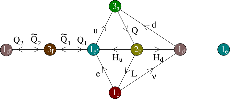
Figure 1: One generation quiver leading to SUSY breaking. This diagram is symmetric with respect to the orientifold O6 plane located on the b stack of branes. Certain mirror nodes are omitted for the sake of simplicity.

The choice of the multiplicity numbers in Table 3 is

$$n=1\qquad n_{u}=1\qquad n_{d}=1\qquad n_{e}=1\qquad n_{\nu}=1\qquad n_{Y}=0\,\,,$$

which satisfies the constraints arising from tadpole cancellation as well as the masslessness of the hypercharge $U(1)_{Y}$ discussed in Section 4. That choice leads for the MSSM spectrum to

$$Q_{L} =(a,b)\qquad u^{c}=(\bar{a},\bar{e})\qquad d^{c}=(\bar{a},d)$$

$$L =(b,\bar{c})\qquad\hskip 2.84526pte^{c}=(c,e)\qquad\nu^{c}=(c,\bar{d})$$

and for the Higgs-meson sector to

$$H_{u}=(b,e)\qquad H_{d}=(b,\bar{d})\qquad M_{1}=(d,\bar{e})\qquad M_{2}=(\bar{d},e)\,\,.$$ (47)

Here the mesons arise after condensation and will be given in terms of $Q$ and $\widetilde{Q}$

$$M_{1}=\widetilde{Q}_{1}\,Q_{2}\qquad\text{and}\qquad M_{2}=\widetilde{Q}_{2}\,Q_{1}\,\,.$$ (48)

The perturbative superpotential is given by all closed loops in the quiver diagram, where one can jump from a node $x$ to its orientifold image changing the orientation of the loop. Let us perform the analysis concretely for the superpotential in the Higgs-meson sector, which is given by

$$W_{0}=\mu\,M_{1}H_{u}H_{d}+m\,M_{1}M_{2}+{\Lambda^{5}\over M_{1}M_{2}}\,\,.$$ (49)

From Figure 1 one can easily see that the term $M_{1}\,M_{2}$ indeed represents a closed loop (from e’ to d’ and back) in the quiver diagram. The superpotential term $M_{1}H_{u}H_{d}$ requires a little bit more work. Let us start at node $b$ and go to node $e^{\prime}$, which describes the $H_{u}$ field. From node $e^{\prime}$ we go via node $f$ to node $d^{\prime}$ and pick up the meson $M_{1}$. To close the loop we jump to the node which is the orientifold image of $d^{\prime}$, namely node $d$ but keeping in mind that such a jump implies reversing the orientation of the loop. Then one can close the loop with the inclusion of $H_{d}$. The last term in (49) is the non-perturbative ADS superpotential term . Note that the superpotential in the Higgs-meson sector is of the type (12) discussed in Section 3.1. There we showed that for a particular choice in parameter space the vacuum breaks SUSY as well as the electroweak gauge symmetry.

Analogously to the Higgs-meson sector, one can determine the superpotential containing the chiral MSSM superfields. Again that corresponds to finding all closed loops involving two quark and lepton fields in the quiver diagram 1. One obtains for the quiver potential

$$W_{2}=Q_{L}H_{u}u^{c}+Q_{L}H_{d}d^{c}+\frac{1}{\Lambda}M_{1}LH_{d}e^{c}+\frac{1}{\Lambda}M_{1}LH_{u}\nu^{c}\,\,.$$ (50)

For simplicity we omit dimensionless couplings. This superpotential generates mass terms for quark and leptons. Interestingly, the origin of masses for quark and leptons in (50) are very different. Masses for the quarks arise from the familiar Yukawa couplings with the MSSM Higgs fields while those for the leptons arise from the quartic couplings involving a meson field. More precisely, at a SUSY breaking vacuum of the type we discussed above this superpotential generates masses for the quarks of order $h_{u,d}$ and for the leptons of order $x_{1}h_{u,d}$. In addition soft SUSY breaking masses for the sparticles follow from non-trivial vevs of the F-fields $\vec{F}_{X}$.

Three generation quiver

The three generation quiver is displayed in Figure 2 and given by the multiplicity choice

$$n=3\qquad n_{u}=2\qquad n_{d}=2\qquad n_{e}=2\qquad n_{\nu}=2\qquad n_{Y}=0$$

which gives the MSSM spectrum

$$\hskip 15.649ptQ_{L}=3\times(a,b)\hskip 28.45274ptu^{c}_{1,2}=2\times(\bar{a},\bar{e})\hskip 31.29802ptu^{c}_{3}=1\times(\bar{a},\bar{d})$$

$$\hskip 14.22636ptd^{c}_{1,2}=2\times(\bar{a},d)\hskip 34.1433ptd^{c}_{3}=1\times(\bar{a},e)\hskip 34.1433ptL=3\times(b,\bar{c})$$

$$e^{c}_{1} =1\times(c,d)\hskip 22.76219pte^{c}_{2,3}=2\times(c,e)\hskip 22.76219pt\nu^{c}_{1}=1\times(c,\bar{e})\hskip 22.76219pt\nu^{c}_{2,3}=2\times(c,\bar{d})\,\,.$$

Let us stress that the choice of multiplicities do pass all the string consistency constraints derived in Section 4. The Higgs-meson sector is the same as for the one generation configuration, see equation (47). Thus it exhibits the same superpotential (49) as for the one generation quiver and therefore as shown in Section 3.1 leads to simultaneous SUSY and electroweak gauge symmetry breaking.

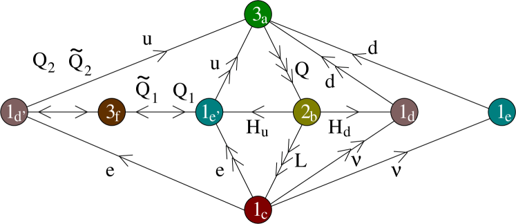
Figure 2: Three generation quiver leading to SUSY breaking.

Finding all closed loops containing exactly two fields $\vec{X}$ gives the MSSM superpotential

$$W_{2}= Q_{L}H_{u}u^{c}_{1,2}+Q_{L}\,H_{d}\,d^{c}_{1,2}+L\,H_{d}\,e^{c}_{1}+L\,H_{u}\,\nu^{c}_{1}$$ (51)

$$\hskip 14.22636pt+\frac{M_{1}}{\Lambda}\Big{(}Q_{L}H_{u}u^{c}_{3}+Q_{L}\,H_{d}\,d^{c}_{3}+L\,H_{d}\,e^{c}_{2,3}+L\,H_{u}\,\nu^{c}_{2,3}\Big{)}\,\,.$$

After the Higgs fields and $M_{1}$ acquire non-zero vev’s this superpotential gives a mass to all the SM fields. In (51) the Yukawa couplings for different families have different coefficients and this might be of use to account for the observed mass hierarchies in the standard model. Note also that this quiver does not contain any R-parity violating couplings or dangerous dimension five operators.

We remark that the perturbative presence of a Dirac neutrino mass term (of the order of the SM mass scale), in conjunction with the presence of a large Majorana mass term for the right-handed neutrinos, induced by a D-instanton, might lead to a neutrino mass of the right size via the seesaw mechanism [42, 43, 44, 45, 46, 47, 48, 49].

Finally let us comment on the mass of $U(1)_{d}$ and $U(1)_{e}$. Only their sum satisfies the constraints for a massless $U(1)$. That implies that both $U(1)_{d}$ and $U(1)_{e}$ become massive via the CS-coupling. This mass crucially depends on the details of the compactification (string coupling, string mass, volume of the cycles the D-branes wrap as well as on the gauge flux living on them, etc.) [50, 51, 52, 53]. Here we assume that both masses are below the scale $\Lambda$, such that at the energy scale $\Lambda$ one has to treat them as an abelian gauge symmetry.

5.2 Second Example

Figures 3 and 4 display the quiver diagrams for a one and three generation configuration, which exhibit a superpotential of the type (33). Let us start again with the one generation quiver.

One generation quiver

Figure 3: One generation quiver with additional an $Y$ leading to SUSY breaking.

For the one generation model the multiplicity numbers in Table 3 are chosen

$$n=1\qquad n_{u}=1\qquad n_{d}=0\qquad n_{e}=0\qquad n_{\nu}=0\qquad n_{Y}=1$$

and lead to the MSSM spectrum

$$Q_{L} =(a,b)\qquad u^{c}=(\bar{a},\bar{e})\qquad d^{c}=(\bar{a},e)$$

$$L =(b,\bar{c})\qquad\hskip 2.84526pte^{c}=(c,d)\qquad\nu^{c}=(c,\bar{e})$$

and to the Higgs-meson spectrum

$$H_{u} =(b,e)\hskip 14.22636ptH_{d}=(b,\bar{d})\hskip 14.22636ptY=(d,\bar{e})\hskip 14.22636ptM_{1}=(d,\bar{e})\hskip 14.22636ptM_{2}=(\bar{d},e)$$ (52)

where again $M_{1}$ and $M_{2}$ denote the mesons after the condensation of $SU(3)_{H}$.

The superpotential is given by all possible loops in the quiver and takes, in the Higgs-meson sector, the form

$$W_{0}=\mu\,M_{1}H_{u}H_{d}+\mu_{Y}\,YH_{u}H_{d}+m\,M_{1}M_{2}+m_{Y}\,YM_{2}+\frac{\Lambda^{5}}{M_{1}\,M_{2}}\,\,.$$ (53)

This is exactly the superpotential analysed in Section 3.2, where it has been shown that for some choice of parameters there exist a SUSY and electroweak gauge symmetry breaking vacuum.

One moreover obtains the desired MSSM Yukawa couplings

$$W_{2}=Q_{L}\,H_{u}\,u^{c}+\frac{1}{\Lambda}\,Q_{L}\,H_{d}\Big{(}M_{1}+Y\Big{)}\,d^{c}+L\,H_{d}\,e^{c}+L\,H_{u}\,\nu^{c}$$ (54)

which gives masses to all the MSSM matter fields after $H_{u}$, $H_{d}$, $M_{1}$ and $Y$ acquire a non-zero vev.

Three-generation quiver

An extension of the above discussed configuration to three families is given by the following choice for the multiplicities in Table 3

$$n=3\qquad n_{u}=2\qquad n_{d}=2\qquad n_{e}=2\qquad n_{\nu}=3\qquad n_{Y}=1\,\,,$$

where again this choice of multiplicities satisfies the string consistency constraints, tadpole cancellation and masslessness of $U(1)_{Y}$. With that choice one obtains the MSSM spectrum

$$Q_{L} =3\times(a,b)\hskip 28.45274ptu^{c}_{1,2}=2\times(\bar{a},\bar{e})\hskip 45.5244ptu^{c}_{3}=1\times(\bar{a},\bar{d})$$

$$d^{c}_{1,2} =2\times(\bar{a},d)\hskip 35.56593ptd^{c}_{3}=1\times(\bar{a},e)\hskip 46.94704ptL=3\times(b,\bar{c})$$ (55)

$$e^{c}_{1} =1\times(c,d)\hskip 31.29802pte^{c}_{2,3}=2\times(c,e)\hskip 31.29802pt\nu^{c}_{1,2,3}=3\times(c,\bar{d})\,\,,$$

while the Higgs-meson sector is the same as for the one generation configuration, see equation (52).

The corresponding quiver is displayed in Figure 4 and the superpotential for the Higgs-meson sector is again given by (53). Thus as shown in Section 3.2 there exists a vacuum which breaks SUSY and also $SU(2)\times U(1)_{Y}$ gauge symmetry.

Figure 4: Three generation quiver with additional an $Y$ leading to SUSY breaking.

The MSSM superpotential is given by

$$W_{2}= Q_{L}H_{u}u^{c}_{1,2}+Q_{L}\,H_{d}\,d^{c}_{1,2}+L\,H_{d}\,e^{c}_{1}$$ (56)

$$\hskip 14.22636pt+\frac{1}{\Lambda}\,\Big{(}M_{1}+Y\Big{)}\Big{(}Q_{L}H_{u}u^{c}_{3}+Q_{L}\,H_{d}\,d^{c}_{3}+L\,H_{d}\,e^{c}_{2,3}+L\,H_{u}\,\nu^{c}_{1,2,3}\Big{)}\,\,.$$

After the Higgs-meson fields acquire a vev all SM fields get a mass. As in the previous example, the fact that one of the families of the right-handed quarks has a different string origin with respect to the other two generations may account for the observed mass hierarchies in the MSSM. As before the quiver does not contain any R-parity violating couplings or dangerous dimension five operators. Moreover, D-instantons can generate large Majorana masses for the right-handed neutrinos. Then the small neutrino masses can be explained via the seesaw mechanism.

As before we assume that the masses of the $U(1)_{d}$ and $U(1)_{e}$ induced by the CS-couplings are below the scale $\Lambda$. That forces us to treat the symmetries $U(1)_{d}$ and $U(1)_{e}$ as gauge symmetries at the energy scale $\Lambda$.

6 Summary

We discussed two extensions of the MSSM which lead, for a large region in parameter space, to SUSY and electroweak gauge symmetry breaking. Both these extensions contain a hidden $SU(3)_{H}$ that condensates via the generation of an ADS superpotential. The condensates (mesons) couple to the Higgs sector which mediates the SUSY and electroweak gauge symmetry breaking to MSSM matter content. In Section 3 we show explicitly that, depending on the region in parameter space, these extensions can give rise to different vacua, that do or do not break SUSY and/or electroweak gauge symmetry. There are large region in parameter space for which both symmetries are broken.

Later in Section 5 we present local D-brane configurations which satisfy severe string consistency constraints and mimic the previously discussed field theory setups. They exhibit the required superpotential to break SUSY and electroweak gauge symmetry. Moreover, all MSSM Yukawa couplings are realized and these configurations can naturally explain some of the observed mass hierarchies of the MSSM.

In this work we assumed that the closed string sector is stabilized thus we ignore all closed string dynamics. Specifically all Yukawa, gauge couplings and Fayet-Iliopoulos terms are input parameters. It would be nice to find a global realization of these local D-brane configurations in which one can study whether moduli stabilization indeed give the Yukawa and gauge couplings, as well as Fayet-Iliopoulos terms in a range that eventually leads to SUSY and gauge symmetry breaking.

Acknowledgments The authors wish to thank P. Anastasopoulos, M. Bianchi, E. Dudas and M. Serone for useful discussions. This work was partially supported by the ERC Advanced Grant n.226455 “Superfields”, by the Italian MIUR-PRIN contract 20075ATT78 and by the NATO grant PST.CLG.978785.

References

- [1] R. N. Mohapatra, Unification and Supersymmetry,. Berlin, Springer (2002) 448 p.
- [2] M. Drees, Theory and Phenomenology of Sparticles,. Singapore, World Sci. Pub. Co. (2005) 584 p.
- [3] J. Terning, Modern supersymmetry: Dynamics and duality,. Oxford, UK: Clarendon (2006) 324 p.
- [4] H. Baer and X. Tata, Weak Scale Supersymmetry,. Cambridge, UK: Cambridge Univ. Pr. (2006) 556 p.
- [5] P. M. R. Binetruy, Supersymmetry,. Oxford, Oxford Univ. Pr. (2007) 536 p.
- [6] M. Dine, Supersymmetry and string theory: Beyond the standard model,. Cambridge, UK: Cambridge Univ. Pr. (2007) 515 p.
- [7] I. Affleck, M. Dine, and N. Seiberg, Exponential hierarchy from dynamical supersymmetry breaking, Phys. Lett. B140 (1984) 59.
- [8] I. Affleck, M. Dine, and N. Seiberg, Dynamical Supersymmetry Breaking in Four-Dimensions and Its Phenomenological Implications, Nucl. Phys. B256 (1985) 557.
- [9] D. Amati, K. Konishi, Y. Meurice, G. C. Rossi, and G. Veneziano, Nonperturbative Aspects in Supersymmetric Gauge Theories, Phys. Rept. 162 (1988) 169–248.
- [10] M. A. Shifman and A. I. Vainshtein, Instantons versus supersymmetry: Fifteen years later, arXiv:hep-th/9902018.
- [11] M. Dine and A. E. Nelson, Dynamical supersymmetry breaking at low-energies, Phys. Rev. D48 (1993) 1277–1287, arXiv:hep-ph/9303230.
- [12] M. Dine, A. E. Nelson, and Y. Shirman, Low-energy dynamical supersymmetry breaking simplified, Phys. Rev. D51 (1995) 1362–1370, arXiv:hep-ph/9408384.
- [13] M. Dine, A. E. Nelson, Y. Nir, and Y. Shirman, New tools for low-energy dynamical supersymmetry breaking, Phys. Rev. D53 (1996) 2658–2669, arXiv:hep-ph/9507378.
- [14] M. Bianchi, F. Fucito, and J. F. Morales, Dynamical supersymmetry breaking from unoriented D-brane instantons, JHEP 08 (2009) 040, arXiv:0904.2156 [hep-th].
- [15] D. Lüst, Intersecting brane worlds: A path to the standard model?, Class. Quant. Grav. 21 (2004) S1399–1424, arXiv:hep-th/0401156.
- [16] A. M. Uranga, Intersecting brane worlds, Class. Quant. Grav. 22 (2005) S41–S76.
- [17] R. Blumenhagen, M. Cvetič, P. Langacker, and G. Shiu, Toward realistic intersecting D-brane models, Ann. Rev. Nucl. Part. Sci. 55 (2005) 71–139, arXiv:hep-th/0502005.
- [18] R. Blumenhagen, B. Körs, D. Lüst, and S. Stieberger, Four-dimensional String Compactifications with D-Branes, Orientifolds and Fluxes, Phys. Rept. 445 (2007) 1–193, arXiv:hep-th/0610327.
- [19] F. Marchesano, Progress in D-brane model building, Fortsch. Phys. 55 (2007) 491–518, arXiv:hep-th/0702094.
- [20] S. Kachru, R. Kallosh, A. D. Linde, and S. P. Trivedi, De Sitter vacua in string theory, Phys. Rev. D68 (2003) 046005, arXiv:hep-th/0301240.
- [21] E. Dudas and S. K. Vempati, Large D-terms, hierarchical soft spectra and moduli stabilisation, Nucl. Phys. B727 (2005) 139–162, arXiv:hep-th/0506172.
- [22] E. Dudas, C. Papineau, and S. Pokorski, Moduli stabilization and uplifting with dynamically generated F-terms, JHEP 02 (2007) 028, arXiv:hep-th/0610297.
- [23] E. Dudas, Y. Mambrini, S. Pokorski, and A. Romagnoni, Moduli stabilization with Fayet-Iliopoulos uplift, JHEP 04 (2008) 015, arXiv:0711.4934 [hep-th].
- [24] M. Cvetič, J. Halverson, and R. Richter, Realistic Yukawa structures from orientifold compactifications, JHEP 12 (2009) 063, arXiv:0905.3379 [hep-th].
- [25] M. Bianchi and J. F. Morales, Anomalies and tadpoles, JHEP 03 (2000) 030, arXiv:hep-th/0002149.
- [26] T. P. T. Dijkstra, L. R. Huiszoon, and A. N. Schellekens, Supersymmetric Standard Model Spectra from RCFT orientifolds, Nucl. Phys. B710 (2005) 3–57, arXiv:hep-th/0411129.
- [27] L. E. Ibáñez and R. Richter, Stringy Instantons and Yukawa Couplings in MSSM-like Orientifold Models, JHEP 03 (2009) 090, arXiv:0811.1583 [hep-th].
- [28] G. K. Leontaris, Instanton induced charged fermion and neutrino masses in a minimal Standard Model scenario from intersecting D- branes, arXiv:0903.3691 [hep-ph].
- [29] P. Anastasopoulos, E. Kiritsis, and A. Lionetto, On mass hierarchies in orientifold vacua, JHEP 08 (2009) 026, arXiv:0905.3044 [hep-th].
- [30] E. Kiritsis, M. Lennek, and B. Schellekens, SU(5) orientifolds, Yukawa couplings, Stringy Instantons and Proton Decay, arXiv:0909.0271 [hep-th].
- [31] M. Cvetič, J. Halverson, and R. Richter, Mass Hierarchies from MSSM Orientifold Compactifications, JHEP 07 (2010) 005, arXiv:0909.4292 [hep-th].
- [32] M. Cvetič, J. Halverson, P. Langacker, and R. Richter, The Weinberg Operator and a Lower String Scale in Orientifold Compactifications, arXiv:1001.3148 [hep-th].
- [33] P. Anastasopoulos, G. K. Leontaris, and N. D. Vlachos, Phenomenological analysis of D-brane Pati-Salam vacua, JHEP 05 (2010) 011, arXiv:1002.2937 [hep-th].
- [34] M. Cvetič, J. Halverson, and P. Langacker, Singlet Extensions of the MSSM in the Quiver Landscape, arXiv:1006.3341 [hep-th].
- [35] R. Blumenhagen, A. Deser, and D. Lüst, FCNC Processes from D-brane Instantons, arXiv:1007.4770 [hep-th].
- [36] I. Antoniadis, E. Kiritsis, and T. N. Tomaras, A D-brane alternative to unification, Phys. Lett. B486 (2000) 186–193, arXiv:hep-ph/0004214.
- [37] G. Aldazabal, L. E. Ibáñez, F. Quevedo, and A. M. Uranga, D-branes at singularities: A bottom-up approach to the string embedding of the standard model, JHEP 08 (2000) 002, arXiv:hep-th/0005067.
- [38] I. Antoniadis, E. Kiritsis, and T. Tomaras, D-brane Standard Model, Fortsch. Phys. 49 (2001) 573–580, arXiv:hep-th/0111269.
- [39] G. Aldazabal, S. Franco, L. E. Ibáñez, R. Rabadan, and A. M. Uranga, D = 4 chiral string compactifications from intersecting branes, J. Math. Phys. 42 (2001) 3103–3126, arXiv:hep-th/0011073.
- [40] L. E. Ibáñez, F. Marchesano, and R. Rabadan, Getting just the standard model at intersecting branes, JHEP 11 (2001) 002, arXiv:hep-th/0105155.
- [41] N. Akerblom, R. Blumenhagen, D. Lust, E. Plauschinn, and M. Schmidt-Sommerfeld, Non-perturbative SQCD Superpotentials from String Instantons, JHEP 04 (2007) 076, arXiv:hep-th/0612132.
- [42] L. E. Ibáñez and A. M. Uranga, Neutrino Majorana masses from string theory instanton effects, JHEP 03 (2007) 052, arXiv:hep-th/0609213.
- [43] R. Blumenhagen, M. Cvetic, and T. Weigand, Spacetime instanton corrections in 4D string vacua - the seesaw mechanism for D-brane models, Nucl. Phys. B771 (2007) 113–142, arXiv:hep-th/0609191.
- [44] R. Argurio, M. Bertolini, G. Ferretti, A. Lerda, and C. Petersson, Stringy Instantons at Orbifold Singularities, JHEP 06 (2007) 067, arXiv:0704.0262 [hep-th].
- [45] M. Bianchi, F. Fucito, and J. F. Morales, D-brane Instantons on the orientifold, JHEP 07 (2007) 038, arXiv:0704.0784 [hep-th].
- [46] L. E. Ibáñez and A. M. Uranga, Instanton Induced Open String Superpotentials and Branes at Singularities, JHEP 02 (2008) 103, arXiv:0711.1316 [hep-th].
- [47] L. E. Ibáñez, A. N. Schellekens, and A. M. Uranga, Instanton Induced Neutrino Majorana Masses in CFT Orientifolds with MSSM-like spectra, JHEP 06 (2007) 011, arXiv:0704.1079 [hep-th].
- [48] M. Cvetič, R. Richter, and T. Weigand, Computation of D-brane instanton induced superpotential couplings - Majorana masses from string theory, Phys. Rev. D76 (2007) 086002, arXiv:hep-th/0703028.
- [49] M. Cvetič and T. Weigand, Hierarchies from D-brane instantons in globally defined Calabi-Yau Orientifolds, Phys. Rev. Lett. 100 (2008) 251601, arXiv:0711.0209 [hep-th].
- [50] I. Antoniadis, E. Kiritsis, and J. Rizos, Anomalous U(1)s in type I superstring vacua, Nucl. Phys. B637 (2002) 92–118, arXiv:hep-th/0204153.
- [51] P. Anastasopoulos, Anomalous U(1)s masses in non-supersymmetric open string vacua, Phys. Lett. B588 (2004) 119–126, arXiv:hep-th/0402105.
- [52] P. Anastasopoulos, M. Bianchi, E. Dudas, and E. Kiritsis, Anomalies, anomalous U(1)’s and generalized Chern-Simons terms, JHEP 11 (2006) 057, arXiv:hep-th/0605225.
- [53] P. Anastasopoulos et al., Minimal Anomalous U(1) -prime Extension of the MSSM, Phys. Rev. D78 (2008) 085014, arXiv:0804.1156 [hep-th].