Abstract

It is proposed to use apertures with large acceptance angles to reduce the integration time when studying the emissivity of laser induced plasmas by means of the Abel inversion method. The spatial resolution lost due to contributions of angled lines of sight to the intensity data collected along the plasma plume diameter is restored by a special numerical data processing. The procedure is meant for the laser induced plasma diagnostics and tomography when the integration time needed to achieve a reasonable signal to noise ratio exceeds a characteristic time scale of the plasma state variations which is short especially at early stages of the plasma evolution.

1 LIBS plasma tomography experiments

Laser-induced breakdown spectroscopy (LIBS) is widely used for quantitative chemical analysis of an elemental content of various materials [1, 2]. A typical experimental setup (see, e.g., [3, 4, 5]) is depicted in Fig. 1. A plasma plume is created by a laser ablation at the distance of two focal lengths from a lens. The lens projects the plasma plume image onto the image plane where a detecting device is placed (e.g., a spectrometer slit). The plasma plume expands, cools, and radiates. All photons propagating along a particular line of sight parallel to a vector ${\bf e}$ through a point at the distance $y$ from the plasma plume symmetry axis can be collected at the point $(0,-y,4f)$, e.g., by a spectrometer slit. The intensity $I_{\Omega}(y)$ measured at the point $(0,-y,4f)$ depends on the solid angle $\Omega$ in which the light is collected. If $\Omega$ is small, then the intensity $I_{\Omega}(y)$ can be approximately viewed as the intensity $I(y)$ in (nearly) parallel lines of sight. In this approximation, the measured intensity is related to the plasma emissivity by the Abel integral equation that can be solved to recover the emissivity [6]. For this reason, spectrometers used in these measurements must have a high $f-$number in order to restrict the solid angle of the acceptance cone. The latter implies, in particular, a small amplitude of the measured signal per unit time. In turn, a long integration time is required to achieve a reasonable signal to noise ratio. If the plasma plume remained stationary during the integration time, the reconstructed emissivity (as well as the plasma temperature distribution and local densities of electrons, ions, and atoms) would have corresponded to the true (instantaneous) plasma parameters. It appears, however, the plasma plume cannot be viewed as stationary during a typical integration time of $1\mu s$ or higher. This is especially true for early stages of the plasma plume evolution [7, 8].

Here the following possibilities are discussed to reduce the integration time. If the plasma plume has the spherical symmetry (or, at least it can be approximated as such), then it is shown that any device with an arbitrary large acceptance cone can be used to collect the data. In particular, spectrometers with low $f-$numbers can be used. The loss of the spatial resolution due to contributions of angled lines of sight into the data function $I_{\Omega}(y)$ can be eliminated by a proposed numerical data processing such that the intensity $I(y)$ in parallel lines of sight is accurately recovered and can be used in the subsequent Abel inversion to obtain the plasma emissivity. The data processing is particularly simple if the device acceptance cone is slightly restricted by a large aperture of a special shape (see Section 3) placed in the lens focal plane (as depicted in Fig. 1). But with minor modifications the reconstruction algorithm is shown to work for any acceptance cone of the measuring device (or any aperture).

If the plasma plume has the axial symmetry, then a measuring device may also have an arbitrary large acceptance cone, but the lines of sights that are not perpendicular to the plasma plume symmetry axis must be blocked by an aperture in the focal plane whose dimension along the symmetry axis is sufficiently small. In other words, only lines of sight that lie within a thin slice of the plasma plume (normal to the symmetry axis) contribute to the measured intensity. This is similar to the conventional experimental setup (e.g., a spectrometer with a high $f-$number). The difference is that photons propagating along all angled lines of sight within the plasma plume slice can be collected to amplify the measured signal. A simple numerical data processing algorithm is proposed to accurately recover the intensity in parallel lines of sight.

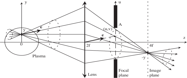
Figure 1: A typical experimental setup for LIBS plasma measurements. A plasma plume is created by a laser ablation at the distance of two focal length from a lens. The light intensity is measured in the image plane. An aperture is placed in the lens focal plane. It restricts the acceptance cone at each point where the intensity is measured (provided the acceptance cone of the light collecting device is wider than that of the aperture). Photons propagating along any particular line of sight parallel to ${\bf e}={\bf e}_{\theta,\varphi}$ that lies within the solid angle of the acceptance cone and goes though the point $(0,y,0)$ in the plasma plume are collected at the point $(0,-y,4f)$. The measurements give the intensity $I_{\Omega}(y)$ as a function of $y$. For large acceptance cones, $I_{\Omega}(y)$ cannot be viewed as the intensity in parallel lines of sight and, hence, cannot be directly used in the Abel inversion to reconstruct the plasma emissivity.

So, a rational behind the use of larger apertures is a reduction of the integration time. This is especially important when studying such a dynamical object as laser-induced plasmas. The plasma diagnostics and tomography based on the Abel inversion becomes inaccurate when the integration times exceeds a characteristic time scale of the plasma state variations which is short especially at early stages of the plasma evolution (e.g., a few $ns$ after the ablation process is over). The method proposed below would allow for a sufficient signal to noise ratio with integration times in the range of $10$’s to $100$’s $ns$ at the price of loosing a spectral resolution. It also allows for the use of spectrometers with low $f-$numbers, which reduces the integration time, but not as much as in the case when the spectral resolution is not needed.

2 A generalized Abel equation for apertures with a large acceptance angle

Suppose that a plasma plume is created on the optical axis of a lens that is at a distance of two focal lengths from the plume (see Fig. 1). Then an image of the plasma plume is created in the plane normal to the optical axis that is at the distance of two focal lengths but on the other side of the lens. Let the plasma emissivity be given as a function of the position vector ${\bf r}$, $\varepsilon=\varepsilon({\bf r})$. The question to be studied is the amount of plasma radiation that can be collected at a point in the image plane. The coordinate system is set so that the optical axis coincides with the $z-$axis. Consider an infinitesimal area element $d\sigma=dxdz$ at the point $(0,y,0)$ (the origin is inside the plasma plume) normal to the $z-$ axis. Let ${\bf e}_{\theta,\varphi}=(\cos\varphi\sin\theta,\,\sin\varphi\sin\theta,\,\cos\theta)$ be the unit vector that defines the direction of a line of sight through the point $(0,y,0)$. The geometrical meaning of the angles $\theta$ and $\varphi$ is transparent. The line has the angle $\theta$ with the optical axis. Variations of $\varphi$ correspond to lines that lie on the cone of the angle $\theta$ whose the axis passes through $(0,y,0)$ and is parallel to the optical axis. By letting $\theta$ and $\varphi$ range over the intervals $[0,\pi/2]$ and $[0,2\pi]$, respectively, all lines of sight through the point $(0,y,0)$ in the plasma plume are parameterized. Without any restriction on the lens diameter, all such lines intersect at the point $(0,-y,4f)$ in the image plane, where $f$ is the lens focal length.

A lens has a finite size and yet it is subject to optical aberration effects. For this reason a diaphragm should be placed in the lens focal plane (see Fig. 1). The diaphragm aperture restricts the ”emission” solid angle within which the light can be collected at the point $(0,-y,4f)$. As noted before, spectrometers with high $f-$numbers are used to collect the light (the spectrometer slit is placed in the image plane parallel to the $y-$ axis). For a high $f-$number, the spectrometer acceptance solid angle is smaller than the ”emission” solid angle. So, not all the plasma radiation that arrives at the observation point is collected. If the acceptance solid angle is small, then the measured intensity is proportional to the intensity in (nearly) parallel lines of sight going through the plasma plume diameter (see below) that is used in the Abel inversion method.

Let us put aside the question about how exactly the light is collected at the point $(0,-y,4f)$ and assume that all the light coming through the aperture can somehow be collected. Alternatively, one can think of any measuring device that has a large acceptance cone. As is clear from Fig. 1, any acceptance cone is equivalent to some aperture placed in the lens focal plane. So, measuring devices and apertures restricting the ”emission” cone can be discussed on the same footing.

The energy collected per unit time, unit frequency, and unit area that was emitted into a solid angle $d\Omega$ in the direction of ${\bf e}_{\theta,\varphi}$ reads [9]

$$I_{\Omega}(y)=\int_{\Omega}d\Omega\cos\theta\int_{-\infty}^{\infty}ds\,\varepsilon\Bigl{(}{\bf r}_{\theta,\varphi}(s,y)\Bigr{)}\equiv\int_{\Omega}d\Omega\cos\theta\ I(\theta,\varphi,y)\,,$$ (1)

where the dependence on the frequency and time is not explicitly shown (it is not relevant for what follows), ${\bf r}_{\theta,\varphi}(s,y)=(0,y,0)+{\bf e}_{\theta,\varphi}s$ is the parametric equation of the line of sight through the point $(0,y,0)$ and parallel to the unit vector ${\bf e}_{\theta,\varphi}$, $s$ is the arclength parameter, $d\Omega=d\theta d\varphi\sin\theta$, and the range for the angles $\theta$ and $\varphi$ is determined by the shape of the aperture in the focal plane. The function $I(\theta,\varphi,y)$ is the light intensity along the line of sight parallel to ${\bf e}_{\theta,\varphi}$ through the point $(0,y,0)$ in the plasma plume. To find the dependence of $I_{\Omega}$ on the aperture geometry, the integration over the solid angle is transformed to a double integral over the aperture by a change of variables. Let $(u,v)$ be rectangular coordinates in the focal plane such that the origin lies on the lens optical axis and the $u-$axis is parallel to the $y-$axis (see Fig. 1). If $dA=dudv$ is the area element at the aperture point $(u,v)$, then

$$d\Omega=\frac{dA\cos\theta}{f^{2}+u^{2}+v^{2}}$$

and the relation between the angles and rectangular coordinates in the focal plane is given by

$$v=f\tan\theta\cos\varphi\,,\quad u=f\tan\theta\sin\varphi\,.$$ (2)

Equation (1) can be written in the form

$$I_{\Omega}(y)=\int_{A}dA\ \frac{f^{2}}{(f^{2}+u^{2}+v^{2})^{2}}\,I(\theta,\varphi,y)\,,$$ (3)

where the angles $\theta$ and $\varphi$ in the arguments of $I$ are expressed via $u$ and $v$ by inverting relations (2). The integration in (3) is carried out over the aperture area denoted by $A$.

Consider first the case of a spherically symmetric plasma plume (the case of the axial symmetry is discussed in Section 4), i.e., $\varepsilon({\bf r})=\varepsilon(r)$ where $r=|{\bf r}|$. The distance $r_{\theta,\varphi}(y)$ between the line ${\bf r}={\bf r}_{\theta,\varphi}(s,y)$ and the origin (the plasma plume center) is given by the magnitude of the vector that is the cross product $(0,y,0)\times{\bf e}_{\theta,\varphi}$. A simple calculation shows that $r_{\theta,\varphi}(y)=|(0,y,0)\times{\bf e}_{\theta,\varphi}|=y(1-\sin^{2}\theta\sin^{2}\varphi)^{1/2}$ for $y\geq 0$. If $I(0,0,y)=I(y)$ is the intensity along the line of sight parallel to the optical axis, then it follows from the assumption of the spherical symmetry of the plasma plume that

$$I(\theta,\varphi,y)=I(r_{\theta,\varphi}(y))\,,\quad\quad r_{\theta,\varphi}(y)=y\sqrt{1-\sin^{2}\theta\sin^{2}\varphi}$$ (4)

because the intensity along any line of sight through the point $(0,y,0)$ depends only on the distance of that line to the plasma plume center. By making use of relations (2) to express $r_{\theta,\varphi}$ as a function of $u$ and $v$, Eq. (3) can be written in the form

$$I_{\Omega}(y)=\int_{A}dA\ \frac{f^{2}}{(f^{2}+u^{2}+v^{2})^{2}}\,I\Bigl{(}y\mu(u,v)\Bigr{)}\,,\quad\quad\mu(u,v)=\sqrt{\frac{f^{2}+v^{2}}{f^{2}+u^{2}+v^{2}}}\,.$$ (5)

If $A$ is an infinitesimal aperture of the area $\Delta A$ centered on the optical axis, then $I_{\Omega}(y)\approx\Delta\Omega I(y)$ where $\Delta\Omega=\Delta A/f^{2}$. In this case, the data function can be used as the intensity along parallel lines of sight $I(y)\approx I_{\Omega}(y)/\Delta\Omega$ that is related to the plasma emissivity $\varepsilon(r)$ by the the Abel integral equation

$$I(y)=\int_{-\infty}^{\infty}ds\,\varepsilon\Bigl{(}\sqrt{y^{2}+s^{2}}\Bigr{)}=2\int_{y}^{\infty}\frac{dr\,r\,\varepsilon(r)}{\sqrt{r^{2}-y^{2}}}\,.$$ (6)

It can be solved for $\varepsilon(r)$. The procedure is known as the Abel inversion [6]:

$$\varepsilon(r)=-\frac{1}{\pi}\int_{r}^{\infty}dy\ \frac{I^{\prime}(y)}{\sqrt{y^{2}-r^{2}}}=\int_{0}^{\infty}dk\,kJ_{0}(kr)\tilde{I}(k)\,,\quad\quad\tilde{I}(k)=\int_{-\infty}^{\infty}dye^{iky}I(y)\,,$$

where $\tilde{I}(k)$ is the Fourier transform of $I(y)$ and $J_{\nu}$ is the Bessel function of index $\nu=0$. Substituting (6) into the right side of Eq. (5), an analog of the Abel integral equation (6) is obtained for an aperture with a finite acceptance angle. If Eq. (5) can be solved for $I(y)$ for a given $I_{\Omega}(y)$, then a solution to the generalized Abel equation is found by means of the Abel inversion for $I(y)$. In Sections 5 a numerical algorithm is proposed for solving Eq. (5) in the case of an aperture of a special shape. The case of an aperture of a general shape is presented in Section 6. A numerical example of is given in Section 7.

3 The hyperbolic aperture

It turns out that there is a particular shape of the aperture for which Eq. (5) is substantially simplified and becomes convenient for a qualitative analysis of the relation between the intensity in parallel lines of sight $I(y)$ and the data function $I_{\Omega}(y)$ for large apertures.

Let $A$ be symmetric relative to the reflection $u\rightarrow-u$ and let $A_{+}$ be the half of $A$ that lies in the half-plane $u\geq 0$. Then $\int_{A}=2\int_{A_{+}}$ in the right side of Eq. (5). Consider the change of variables in the double integral (5): $(u,v)\rightarrow(\mu,v)$ where the new variable $\mu=\mu(u,v)$ is defined by the second relation in (5). Then $dA=dudv=dvd\mu J$ where the Jacobian is $J=\partial u/\partial\mu=(\partial\mu/\partial u)^{-1}$. The coordinate line $\mu=const$ is a hyperbola in the $(u,v)-$plane:

$$u=\frac{\sqrt{1-\mu^{2}}}{\mu}\sqrt{v^{2}+f^{2}}\,.$$ (7)

It intersects the $u-$axis at $u=f\sqrt{1-\mu^{2}}/\mu$ and has slant asymptotes $u=|v|\sqrt{1-\mu^{2}}/\mu$ at large $|v|$. In particular, the line $u=0$ (or the $v-$axis) is the limiting hyperbola as $\mu\rightarrow 1$. Note that the $u-$intercept of the hyperbola (7) tends to zero, while the slope of the slant asymptotes becomes infinite, i.e., the hyperbola tends to the vertical straight line through $u=0$. Let $A_{+}$ be bounded by horizontal lines $v=\pm\Delta_{a}$, the vertical line $u=0$, and by the hyperbola (7) with $\mu=\mu_{a}<1$ as is shown in the left panel of Fig. 2.

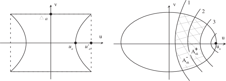
Figure 2: Left panel: A hyperbolic aperture that allows for a factorization in the sum over angled lines of sight. It is bounded by the lines $v=\pm\Delta_{a}$ and hyperbolas $u=\pm\tan\theta_{a}\sqrt{v^{2}+f^{2}}$. Here $u_{a}=f\tan\theta_{a}=f\sqrt{1-\mu_{a}^{2}}/\mu_{a}$ and $u_{a}^{\prime}=\tan\theta_{a}\sqrt{f^{2}+\Delta_{a}^{2}}$. For $\Delta_{a}\sim f$, the aperture cannot be approximated by a rectangle. A rectangular approximation is accurate if $\Delta_{a}\ll f$. It can be used for studies of axially symmetric plasmas as explained in the text. Right panel: An illustration to the reconstruction algorithm for a general aperture. Curves 1, 2, and 3 are the level curves (hyperbolas) $\mu(u,v)=\mu_{nk}^{-}$, $\mu(u,v)=\mu_{nk}^{+}$, and $\mu(u,v)=\mu_{nk+1}^{-}$, respectively, that are used to partition the region occupied by the aperture. In each partition region $A_{nk}^{\pm}$, the function $I_{n}(\mu)$ is approximated by a linear function as is explained in the text. Here $\mu_{a}$ is the minimal value of the function $\mu(u,v)$.

Then after the change of integration variables, the range of new variables is the rectangle $-\Delta_{a}\leq v\leq\Delta_{a}$ and $\mu_{a}\leq\mu\leq 1$. A straightforward calculation shows that the double integral (5) is factorized in the new variables thanks to the ”hyperbolic” shape of the aperture:

$$I_{\Omega}(y)=4\int_{0}^{\Delta_{a}}\frac{dv}{\sqrt{f^{2}+v^{2}}}\int_{\mu_{a}}^{1}\frac{d\mu\,\mu^{2}}{\sqrt{1-\mu^{2}}}\ I(\mu y)=\frac{4\Delta_{a}}{\sqrt{f^{2}+\Delta_{a}^{2}}}\int_{\mu_{a}}^{1}\frac{d\mu\,\mu^{2}}{\sqrt{1-\mu^{2}}}\ I(\mu y)\,.$$ (8)

Put $\mu=\cos\theta$ so that $u=f\tan\theta_{a}\equiv u_{a}$ defines the $u-$intercept of the hyperbola (7) with $\mu=\mu_{a}$ that bounds the aperture area $A_{+}$. Put also $\tan\varphi_{a}=\Delta_{a}/f$. Then

$$I_{\Omega}(y)=4\sin\varphi_{a}\int_{0}^{\theta_{a}}d\theta\cos^{2}\theta\ I(y\cos\theta)\,.$$ (9)

This equation is simple enough to estimate the signal amplification due to an aperture with a large acceptance angle and compare it with signal measurements in reported LIBS plasma tomography experiments [4, 5].

In the conventional LIBS plasma tomography experiments, the slit of a spectrometer is placed into the image plane parallel to $y-$axis. However, not all the light that enters into the spectrometer slit at the point $(0,-y,4f)$ is collected but rather its only portion that illuminates a spectrometer mirror (that further directs the light onto the spectral grating). If the aperture in the focal plane is not too small or not present at all, this portion is determined only by the $f-$number of the spectrometer so that the acceptance solid angle in Eq. (1) is defined by $0\leq\varphi\leq 2\pi$ and $0\leq\theta\leq\theta_{s}$ where $\tan\theta_{s}=1/(2f_{s})$ and $f_{s}$ is the spectrometer $f-$number. Spectrometers in the reported LIBS plasma tomography experiments typically have relatively large $f-$numbers, $f_{s}\sim 5$. So, the acceptance angle is small, $\tan\theta_{s}\approx\theta_{s}\sim 10^{-1}$. It is then sufficient to calculate the integral (1) in the leading order of $\theta_{s}^{2}$, while neglecting terms of order $\theta^{4}_{s}$. In this approximation $I(\theta,\varphi,y)=I(y)+O(\theta^{2})$ (cf. (4)) and the evaluation of the integral (1) yields:

$$I_{\Omega}(y)=\pi\theta_{s}^{2}I(y)+O(\theta^{4}_{s})\,.$$

The smallness of the factor $\pi\theta_{s}^{2}$ in the rate of the energy flux per unit time is exactly the reason to have a long integration time to get a sufficient signal to noise ratio, when determining $I(y)$ used in the Abel inversion. Suppose now that all the light that comes to the point $(0,-y,4f)$ through the hyperbolic aperture is collected. Assuming, for sake of simplicity, $I(y\cos\theta)$ to be a constant $I$, the evaluation of the integral in (9) yields:

$$I_{\Omega}\approx 4\sin\varphi_{a}(2\theta_{a}-\sin(2\theta_{a}))\,I\,.$$

So the signal amplification (as compared to the spectrometer case) can be estimated by a factor of $4\sin\varphi_{a}(2\theta_{a}-\sin(2\theta_{a}))/(\pi\theta_{s}^{2})\sim 50$ if $\theta_{s}\sim 10^{-1}$ and $\varphi_{a}\sim\theta_{a}\sim\pi/4$ (i.e., $\Delta_{a}\sim u_{a}\sim f$).

To increase the angles $\varphi_{a}$ and $\theta_{a}$, spectrometers with small $f-$numbers can be used. An effective aperture corresponding to this case is a circular disk of the radius $f/(2f_{s})$. If the hyperbolic aperture is fit into this disk, then Eq. (9) applies directly, and $I(y)$ is recovered by the numerical data processing proposed in Section 5. Otherwise, a circular aperture should be treated by the algorithm of Section 6.

If the spectral resolution is not needed, then a gated ICCD camera can be placed in the image plane. The pixel row of the camera is set along the plasma image diameter. The light collected by each pixel provides the spatially resolved data $I_{\Omega}(y)$. If the aperture has the hyperbolic shape, Eq. (9) applies directly to recover $I(y)$. Otherwise, the algorithm of Section 6 must be used. To study the plasma emissivity in a narrow frequency window of interest, a narrow band (or interference) filter can be positioned in front of the detector (the pixel array). This method can be particularly useful for diagnostics of laser induced plasmas shortly after the ablation process ($\sim\,10$’s $ns$). At this stage the plasma exhibits a fast dynamics and emits mostly a continuum spectrum radiation.

4 Axially symmetric plasma plumes

For axially symmetric plasma plumes, photons propagating along lines of sight that are not perpendicular to the plume symmetry axis must be prevented from being collected by a detector so that only a plasma plume slice normal to the symmetry axis is visible to a measuring device. For spectrometers with high $f-$ numbers, this is achieved automatically due to their narrow acceptance cones. But a narrow acceptance cone also eliminates most of lines of sight in the visible slice itself that are angled to the optical axis. If $R$ is a plasma plume radius, then the lines of sight through $(0,y,0)$ in the acceptance cone of the angle $\theta_{s}$ can go through plasma points separated at most by the distance $2R\tan\theta_{s}$. This determines the spatial resolution along the $y-$axis (as well as along the symmetry axis). For $\theta_{s}\sim 10^{-1}$, the resolution is such that the data can be collected at about 10 positions across the plasma plume diameter without a significant overlap of the plasma regions from which the light is collected. So, when spectrometers with lower $f-$numbers or pixel rows of an ICCD camera (as suggested above) are used to increase the signal, the spatial resolution become even worse along both the directions, the $y-$ and symmetry axes.

The following compromise can be made. The spatial resolution in the direction parallel to the symmetry axis is achieved by placing a slit-like aperture extended along the $y-$axis in the focal plane. If a slit of height $2\Delta_{a}$ is positioned in the focal plane ($-\Delta_{a}\leq v\leq\Delta_{a}$ in the above notations), then only photons traveling along the lines of sight that are in the plasma ”slice” of height $2R\tan\varphi_{a}=2R\Delta_{a}/f$ can reach the image plane. The shape of a sufficiently narrow rectangular aperture can well be approximated by the hyperbolic aperture with small $\Delta_{a}$ because the hyperbola (7) has the vertical tangent line at the intercept point $u=u_{a}$ (see the caption of Fig. 2). Thus, Eq. (8) or (9) remains applicable in this case, but the angle $\theta_{a}$ is determined by the measuring device $f-$number, i.e., $\tan\theta_{a}=1/(2f_{s})$ (the approximation of a small $\theta_{s}$ is invalid for small $f_{s}$), and $\varphi_{a}$ is small enough to provide for the spatial resolution along the plasma plume symmetry axis.

Two-dimensional detectors used in LIBS experiments [4, 5] in combination with a spectrometer typically have about a few hundred pixels for the spatial resolution along the spectrometer slit, while only 10 to 20 spatially resolved data points are taken (each data point corresponds to an average intensity over a cluster of pixels). The algorithm provided below allows for an accurate reconstruction of the spatial resolution of just a single pixel size. So, it may not be deprived of sense to apply the proposed algorithm to improve the spatial resolution even in spectrometers with higher $f-$numbers. This, however, depends very much on the gradients of thermodynamic parameters of the observed plasma. For high gradients, this is definitely the case.

5 The reconstruction algorithm

Let the light be collected by a linear array of pixel detectors placed along the $y-$axis in the image plane. Each pixel has a size $\Delta$. The pixel centers are located at $y=y_{n}=n\Delta$, $n=0,1,...,N$ (by the symmetry of the observed plasma, it is sufficient to reconstruct $I(y)$ (the intensity in parallel lines of sight) only for non-negative $y$, $I(-y)=I(y)$). In what follows the factor $4\sin\varphi_{a}$ in (9) will be omitted. The energy of all photons collected by a pixel $n$ per unit time and unit frequency is given by

$$I^{\Omega}_{n} = \int_{y_{n-1/2}}^{y_{n+1/2}}dyI_{\Omega}(y)=\int_{\mu_{a}}^{1}\frac{d\mu\,\mu^{2}}{\sqrt{1-\mu^{2}}}\,\int_{y_{n-1/2}}^{y_{n+1/2}}dyI(\mu y)=\int_{\mu_{a}}^{1}\frac{d\mu\,\mu}{\sqrt{1-\mu^{2}}}\,I_{n}(\mu)\quad$$ (10)

$$I_{n}(\mu) = \int_{\mu y_{n-1/2}}^{\mu y_{n+1/2}}du\ I(u)\,,$$ (11)

where $y_{n\pm 1/2}=\Delta(n\pm 1/2)$ are the boundary points of the $n$th pixel, and the change of the integration variable $u=\mu y$ has been carried out. If only the photons propagating along parallel lines of sight were registered by the $n$th pixel, then the data would have consisted of values

$$I_{n}=\int_{y_{n-1/2}}^{y_{n+1/2}}du\ I(u)=I_{n}(1)\,.$$ (12)

Exactly these values must be used in the Abel inversion to reconstruct the emissivity. The idea is to find a suitable interpolation for the functions $I_{n}(\mu)$ using the ”sampling” points $I_{n}$. Then the integral with respect to $\mu$ in (10) can be evaluated thus turning Eq. (10) into a system of algebraic equations for $I_{n}$ that can be solved for a given data set $I_{n}^{\Omega}$.

Let $P_{n}(\mu)$ denote the interval $[\mu y_{n-1/2},\mu y_{n+1/2}]$ so that $P_{n}(1)=P_{n}$ is the interval occupied by the $n$th pixel. Depending on the values of $\mu$ and $n$, the interval $P_{n}(\mu)$ may have the following positions relative to the intervals occupied by physical pixels:

$$P_{n}(\mu)\ {\rm overlaps\ with\ both}\ P_{n-k+1}\ {\rm and}\ P_{n-k},\quad{\rm or}\quad P_{n}(\mu)\ {\rm is\ contained\ in}\ P_{n-k}$$ (13)

for $k=1,2,...,N_{n}$ where $N_{n}=[(1-\mu_{a})n]+1$ and $[x]$ denotes the largest integer that does not exceed $x$. The integer $N_{n}$ is defined by the condition $y_{n-N_{n}}<\mu_{a}y_{n}\leq y_{n-N_{n}+1}$. For a fixed value of $n$ it is not difficult to find the ranges of $\mu$ in both the cases (13):

$$\mu_{nk}^{+}\leq \mu \leq\mu_{nk}^{-}\,,\quad{\rm or}\quad\mu_{nk+1}^{-}\leq\mu\leq\mu_{nk}^{+}\,,$$ (14)

$$\mu_{nk}^{\pm} = \frac{n-k+1/2}{n\pm 1/2}\,,\quad k=1,2,...,N_{n}\,,\quad\mu^{-}_{nN_{n}+1}=\mu_{a}\,.$$ (15)

For example, for $k=1$, the first case in (13) holds as long as $\mu y_{n+1/2}$ remains in $P_{n}$, i.e., $\mu y_{n+1/2}\geq y_{n-1+1/2}$ or $\mu\geq\mu_{n1}^{+}$. As $\mu$ becomes less than $\mu_{n1}^{+}$, the whole interval $P_{n}(\mu)$ remains in $P_{n-1}$ until the left boundary of $P_{n}(\mu)$ crosses the left boundary of $P_{n-1}$, i.e., $\mu y_{n-1/2}\geq y_{n-2+1/2}$ or $\mu\geq\mu_{n2}^{-}$, and so on. A special consideration is required for the case $k=N_{n}$ because, depending on the value of $\mu_{a}$, either both the cases (13), or just the first one, or none of them may occur. This issue will be clarified shortly. For time being, the values $\mu_{nk}^{\pm}$ are defined by (15), i.e., $\mu_{a}$ is assumed not to exceed $\mu_{nN_{n}^{+}}$ (both the cases (13) are possible for $k=N_{n}$).

Consider two integrals $\int_{a}^{b}dx\,f(x)$ and $\int_{a^{\prime}}^{b^{\prime}}dx\,f(x)$ for some $f(x)$ where $a\leq a^{\prime}<b^{\prime}\leq b$. How can the second integral be approximated by the first one? The following approximation is proposed:

$$\int_{a^{\prime}}^{b^{\prime}}dx\,f(x)\approx\frac{b^{\prime}-a^{\prime}}{b-a}\,\int_{a}^{b}dx\,f(x)\,.$$ (16)

The accuracy of this approximation is discussed in Appendix. For a small interval length $b-a$ and smooth $f$, this is a good approximation as is shown in Appendix. If $\mu$ is such that the interval $P_{n}(\mu)$ is contained in $P_{n-k}$, then the approximation (16) applies directly:

$$I_{n}(\mu)=\frac{\mu\Delta}{\Delta}\ I_{n-k}=\mu\,I_{n-k}\,,\quad\mu_{nk+1}^{-}\leq\mu\leq\mu_{nk}^{+}\,.$$ (17)

If $\mu$ is such that $P_{n}(\mu)$ overlaps with $P_{n-k}$ and $P_{n-k+1}$, then $I_{n}(\mu)$ is approximated by a linear combination of $I_{n-k+1}$ and $I_{n-k}$ with the coefficients being the lengths of fractions of $P_{n}(\mu)$ in $P_{n-k+1}$ and $P_{n-k}$, respectively, in units of the pixel size $\Delta$:

$$I_{n}(\mu)=\Bigl{(}\mu a_{n}-a_{n-k}\Bigr{)}I_{n-k+1}+\Bigr{(}\mu(1-a_{n})+a_{n-k}\Bigl{)}I_{n-k}\,,\quad\mu_{nk}^{+}\leq\mu\leq\mu_{nk}^{-}\,,$$ (18)

where $a_{n}=n+1/2$. The integral over the interval $[\mu_{a},1]$ in (10) is split into the sum of integrals over the intervals in which the approximations (17) and (18) hold

$$I_{n}^{\Omega}=\sum_{k=1}^{N_{n}}\left(\int_{\mu_{nk}^{+}}^{\mu_{nk}^{-}}+\int_{\mu_{nk+1}^{-}}^{\mu_{nk}^{+}}\right)\frac{d\mu\,\mu}{\sqrt{1-\mu^{2}}}\ I_{n}(\mu)\,.$$ (19)

The integrals are easily evaluated and the desired system of linear equations for $I_{n}$ is obtained. There is a simple recurrence algorithm to solve it. Before describing it, the issue about the integration limits in the term $k=N_{n}$ must be addressed.

Consider the last three integrals in the sum (19):

$$\int_{\mu_{nN_{n}-1}^{-}}^{\mu_{nN_{n}}^{+}}+\int_{\mu_{nN_{n}}^{+}}^{\mu_{nN_{n}}^{-}}+\int^{\mu_{nN_{n}}^{+}}_{\mu_{a}}\,,$$ (20)

in accord with the definition (15). By examining the possible overlaps of $P_{n}(\mu)$ with $P_{n-N_{n}}$ and $P_{n-N_{n}+1}$ depending on the value of $\mu_{a}$, the following three possibilities are found to occur. If $\mu_{a}\geq\mu_{nN_{n}}^{-}$ where the value of $\mu_{nN_{n}}^{-}$ is computed by the rule (15), then the last two integrals in (20) cannot occur in the sum (19) and must be removed. If $\mu_{nN_{n}}^{+}\leq\mu_{a}<\mu_{nN_{n}}^{-}$ where the values of $\mu_{nN_{n}}^{\pm}$ are calculated by the rule (15), then the very last integral in (20) cannot be present and must be removed from the sum (19). Only if $\mu_{a}<\mu_{nN_{n}}$ all three integrals (20) are present in the sum (20). For algorithm implementation purposes, it is convenient to retain the sum (19) as it is. The above three cases can be accounted for if, after calculating the values of $\mu_{nk}^{\pm}$ by the rule (15), the values of $\mu_{nN_{n}}^{\pm}$ are redefined by the rule:

$$\mu_{nN_{n}}^{-}\rightarrow\max(\mu_{a},\mu_{nN_{n}}^{-})\,,\quad\mu_{nN_{n}}^{+}\rightarrow\max(\mu_{a},\mu_{nN_{n}}^{+})\,.$$

It is straightforward to verify that the unwanted integrals in (20) (and, hence, in (19)) always vanish as their upper and lower limits coincide.

Define the functions

$$F_{0}(\alpha,\beta) = \int_{\alpha}^{\beta}\frac{d\mu\,\mu}{\sqrt{1-\mu^{2}}}=\sqrt{1-\alpha^{2}}-\sqrt{1-\beta^{2}}\,,$$

$$F_{1}(\alpha,\beta) = \int_{\alpha}^{\beta}\frac{d\mu\,\mu^{2}}{\sqrt{1-\mu^{2}}}=\frac{1}{2}\Bigl{(}\cos^{-1}(\alpha)-\cos^{-1}(\beta)\Bigr{)}+\frac{1}{2}\Bigl{(}\alpha\sqrt{1-\alpha^{2}}-\beta\sqrt{1-\beta^{2}}\Bigr{)}\,.$$

They are used to evaluate the integrals in the sum (19). For the central pixel $(n=0)$, one finds

$$I_{0}=\frac{I_{0}^{\Omega}}{F_{1}(\mu_{a},1)}\,.$$ (21)

For $n=1,2,...,N$, Eq. (19) yields the recurrence relation

$$I_{n}=\frac{I_{n}^{\Omega}-I_{n}^{F}}{C_{n1}}\,,$$ (22)

where

$$C_{nk} = F_{1}(\mu_{nk}^{+},\mu_{nk}^{-})a_{n}-F_{0}(\mu_{nk}^{+},\mu_{nk}^{-})a_{n-k}\,,\quad k=1,2,...,N_{n}\,,$$

$$I_{n}^{F} = \sum_{k=2}^{N_{n}}C_{nk}I_{n-k+1}+\sum_{k=1}^{N_{n}}\Bigl{[}F_{1}(\mu_{nk+1}^{-},\mu_{nk}^{-})-C_{nk}\Bigr{]}I_{n-k}\,.$$

Note that $I_{n}^{F}$ depends only on $I_{0}$, $I_{1}$,…,$I_{n-1}$. So by executing the recurrence relation (22) with the initial condition (21), all the values $I_{n}$ are found. They can then be used to determine the emissivity by a suitable Abel inversion algorithm. There is a vast literature on the numerical Abel inversion (see, e.g., [10]), and, for this reason, it will not be discussed here. In Section 7, it is demonstrated that for emissivity functions representative for LIBS plasmas, the proposed algorithm provides a very accurate reconstruction of $I_{n}$. Thus, the accuracy in the emissivity reconstruction would be determined by the accuracy of a particular Abel inversion algorithm.

6 General apertures

It is not difficult to extend the proposed algorithm to an aperture of a generic shape. Suppose that $A$ is symmetric under the reflection $u\rightarrow-u$ and $A_{+}$ is the half of $A$ for which $u\geq 0$. A generalization to the non-symmetric case is trivial. Integrating Eq. (5) over the interval occupied by the $n$th pixel, a generalization of (10) is obtained

$$I_{n}^{\Omega}=2\int_{A_{+}}dA\,\frac{f^{2}}{(f^{2}+u^{2}+v^{2})^{2}}\ I_{n}(\mu(u,v))\,,$$ (23)

where the function $\mu(u,v)$ is defined by the second equation in (5). The area $A_{+}$ can be partitioned into regions that lies between the level curves (hyperbolas) of the function $\mu(u,v)$:

$$\mu(u,v)=\mu_{nk}^{+}\,,\quad\quad\mu(u,v)=\mu_{nk}^{-}\,,$$

where $\mu_{nk}^{\pm}$ are defined in (15) and $\mu_{a}=\min_{A_{+}}\mu(u,v)$. The procedure is shown in the right panel of Fig. 2. Let $A_{nk}^{-}$ and $A_{nk}^{+}$ be the regions in which $\mu_{nk}^{+}\leq\mu(u,v)\leq\mu_{nk}^{-}$ and $\mu_{nk+1}^{-}\leq\mu(u,v)\leq\mu_{nk}^{+}$, respectively. Then a generalization of Eq. (19) to the case of a generic aperture reads

$$I_{n}^{\Omega}=2\sum_{k=1}^{N_{n}}\left(\int_{A_{nk}^{-}}+\int_{A_{nk}^{+}}\right)dA\ \frac{f^{2}}{(f^{2}+u^{2}+v^{2})^{2}}\ I_{n}(\mu(u,v))\,.$$ (24)

The approximations (17) and (18) are used for $I_{n}(\mu)$ in the regions $A_{nk}^{+}$ and $A_{nk}^{-}$, respectively to evaluate the double integrals in (24). Depending of the shape of $A$, it can be done either analytically or numerically. Put

$$F_{m}(B)=2\int_{B}dA\ \frac{f^{2}}{(f^{2}+u^{2}+v^{2})^{2}}\ \mu^{m}(u,v)\,,\quad\quad m=0,1\,,$$

for a planar region $B$. The initial condition (21) and the recurrence relation (22) become

$$I_{0}=\frac{I_{0}^{\Omega}}{F_{1}(A_{+})}\,,\quad I_{n}=\frac{I_{n}^{\Omega}-I_{n}^{F}}{C_{n1}}\,,\quad n=1,2,...,N\,,$$ (25)

where

$$C_{nk} = a_{n}F_{1}(A_{nk}^{-})-a_{n-k}F_{0}(A_{nk}^{-})\,,\quad a_{n}=n+1/2\,,$$

$$I_{n}^{F} = \sum_{k=2}^{N_{n}}C_{nk}I_{n-k+1}+\sum_{k=1}^{N_{n}}\Bigl{(}F_{1}(A_{nk})-C_{nk}\Bigr{)}I_{n-k}\,,$$

and $A_{nk}$ is the union of $A_{nk}^{+}$ and $A_{nk}^{-}$.

7 Numerical results for a hyperbolic aperture

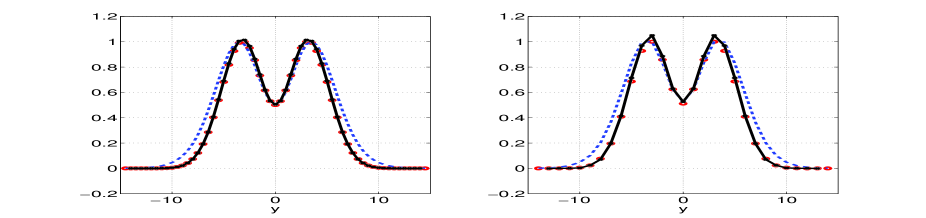
Figure 3: Numerical results for a hyperbolic aperture with $\mu_{a}=\cos\theta_{a}$, $\theta_{a}=51.3^{o}$. Left panel: The solid (black) curve is the graph of the intensity $I(y)$ in parallel lines of sight for the emissivity $\varepsilon(r)$ described in the text. The dashed (blue) curve is the observed intensity $I_{\Omega}(y)$ calculated from $I(y)$ as specified in Eq. (8). Both the curves are normalized on their maximal values. The amplification of the signal is not shown explicitly. It is determined as explained in the text. Solid (red) dots are reconstructed values of $I_{n}$ from $I_{n}^{\Omega}$. The number of pixels is 60 ($N=31$). Right panel: The same as in the left panel but the number of pixels is 30 $(N=16)$. A small inaccuracy of the reconstructed values of $I_{n}$ is observed near the maxima of the intensity $I(y)$ which occurs through errors in the approximations (17) and (18).

The reconstruction algorithm has been tested with synthetic data. The emissivity function is taken in the form $\varepsilon(r)=\varepsilon_{0}\exp(-r^{2}/(2\sigma^{2}))(a-\cos(br))$ where the values of the parameters (arbitrary units) are $\varepsilon_{0}=1$, $\sigma=3$, $a=1.4$, and $b=0.5$. The emissivity profile is typical for the LIBS plasmas observed in experiments [5]. The intensity $I(y)$ in parallel lines of sight is calculated by means of Eq. (6). Then the integral intensity over all lines of sight within the acceptance solid angle defined by the hyperbolic aperture with $\mu_{a}=\cos\theta_{a}$, $\theta_{a}=51.3^{o}$ is found by Eq. (9) (the amplification factor $4\sin\varphi_{a}$ is omitted as it is irrelevant for the reconstruction algorithm). The synthetic data are calculated by means of Eq. (10) when 60 and 30 pixels are placed across the plasma plume diameter. Then the reconstruction algorithm is applied to find the values $I_{n}$. The results are shown in Fig. 3. The left and right panels represent the cases with $60$ and $30$ pixels, respectively. The solid (black) and dashed (blue) curves are the graphs of $I(y)$ and $I_{\Omega}(y)$, respectively. Both the curves are normalized to their maximal values so that the amplification factor due to the vertical size $\Delta_{a}$ of the hyperbolic aperture cannot be seen. This normalization would not make sense for a generic aperture because there is no factorization in the sum over angled lines of sight for apertures of a general shape (see Section 6). Yet, the factorization due to the hyperbolic aperture leads to a mild deviation of $I_{\Omega}(y)$ from $I(y)$ when they are normalized on their maximal values. The solid (red) dots show the reconstructed values of $I_{n}$. The reconstruction is very accurate for the case of $60$ pixels. When the pixel size increases, the approximations (17) and (18) becomes less accurate as proved in Appendix. A reconstruction error increases near the maxima of $I(y)$ when the pixel size is doubled (the right panel of Fig. 3). For a typical pixel detector, the pixel size is about $0.02\,mm$. So, for a typical LIBS plasma plume diameter of $2\,mm$, there are about 100 pixel collecting the data.

A. Appendix

Here the accuracy of the approximation (16) is assessed. For a continuous function $f(x)$ there exist points $a\leq x_{*}\leq b$ and $a^{\prime}\leq x^{\prime}_{*}\leq b^{\prime}$ such that

$$I=\int_{a}^{b}dxf(x)=(b-a)f(x_{*})\,,\quad I^{\prime}=\int_{a^{\prime}}^{b^{\prime}}dxf(x)=(b^{\prime}-a^{\prime})f(x_{*}^{\prime})\,.$$

It follows from these relations that

$$I^{\prime}=\frac{\Delta^{\prime}}{\Delta}\,I+\Delta^{\prime}\Bigl{(}f(x_{*}^{\prime})-f(x_{*})\Bigr{)}\,,$$

where $\Delta=b-a$ and $\Delta^{\prime}=b^{\prime}-a^{\prime}$. By the mean value theorem, the last term in this equality can be transformed so that

$$I^{\prime}=\frac{\Delta^{\prime}}{\Delta}\,I+\Delta^{\prime}(x_{*}^{\prime}-x_{*})f^{\prime}(\xi)\equiv\frac{\Delta^{\prime}}{\Delta}\,I+\gamma$$

for some $\xi$ between $x_{*}^{\prime}$ and $x_{*}$. Therefore the error $\gamma$ is bounded by

$$|\gamma|\leq M\Delta^{\prime}\Delta\,,\quad\quad M=\max_{[a,b]}|f^{\prime}(x)|\,.$$

If $\Delta\rightarrow 0$, while $\Delta^{\prime}/\Delta$ remains finite, the error decreases as $\Delta^{2}$.

References

- [1] I.D. Winefordner, I.B. Gornushkin, T. Correll, E. Gibb, B.W. Smith, N. Omenetto, J. Anal. At. Spectrom. 19, 1061 (2004)
- [2] C. Pasquini, J. Cortez, L.M.C. Silva, F.B. Gonzaga, J. Braz. Chem. Soc. 18, 463 (2007)
- [3] J. W. Olesik and G. M. Hieftje, Anal. Chem. 57, 2049 (1985)
- [4] R. Álvarez, A. Roberto, M. C. Quintero, Spectrochim. Acta B 57, 1665 (2002)
- [5] J. A. Aguilera, C. Aragón, and J. Bengoechea, Appl. Optics 42, 5938 (2003)
-
[6]
A. C. Eckrbeth, Laser diagnostic for
combustion temperature and species, (Gordon & Breach,
Amsterdam, 1996);
H. R. Griem, Principles of plasma spectroscopy (Cambridge University Press, Cambridge, 1997) - [7] A. Casavola, G. Colonna, and M. Capitelli, Appl. Surf. Sci. 208-209, 559 (2003)
- [8] M. Capitelli, F. Capitelli, and A. Eletskii, Spectrochim. Acta B 56, 567 (2001)
- [9] S. Chandrasekhar, Radiative transfer (Dover Publications, New York, 1960)
-
[10]
W. Lochte-Holtgreven, in:
Plasma diagnostics, ed. W. Lochte-Holtgreven
(North-Holland Pub. Co., Amsterdam, 1968), p. 135;
J.D. Algeo and M.B. Denton, Appl. Spectrosc. 35, 35 (1981);
W. R. Wing and R. V. Neidigh, Am. J. Phys. 39, 760 (1971);
R.N. Bracewell, The Fourier transform and its applications (McGraw-Hill Book Co., New York, 1965);
D.R. Keefer, L. Smith, and S.J. Sudhasanan, Abel inversion using transforms techniques (Univ. of Tennessee Space Institute, Tullahoma, 1986)