Handle Addition for doubly-periodic Scherk Surfaces

Abstract.

We prove the existence of a family of embedded doubly periodic minimal surfaces of (quotient) genus $g$ with orthogonal ends that generalizes the classical doubly periodic surface of Scherk and the genus-one Scherk surface of Karcher. The proof of the family of immersed surfaces is by induction on genus, while the proof of embeddedness is by the conjugate Plateau method.

1. Introduction

In this note we prove the existence of a sequence $\{S_{g}\}$ of embedded doubly-periodic minimal surfaces, beginning with the classical Scherk surface, indexed by the number $g$ of handles in a fundamental domain. Formally, we prove

Theorem 1.1.

There exists a family $\{S_{g}\}$ of embedded minimal surfaces, invariant under a rank two group $\Lambda_{g}$ generated by horizontal orthogonal translations. The quotient of each surface $S_{g}$ by $\Lambda_{g}$ has genus $g$ and four vertical ends arranged into two orthogonal pairs.

Our interest in these surfaces has a number of sources. First, of course, is that these are a new family of embedded doubly periodic minimal surfaces with high topological complexity but relatively small symmetry group for their quotient genus. Next, unlike the surfaces produced through desingularization of degenerate configurations (see [24], [25] for example), these surfaces are not created as members of a degenerating family or are even known to be close to a degenerate surface. More concretely, there is now an abundance of embedded doubly periodic minimal surfaces with parallel ends due to [3], while in the case of non-parallel ends, the Scherk and Karcher-Scherk surfaces were the only examples.

Third, one can imagine these surfaces as the initial point for a sheared family of (quotient) genus $g$ embedded surfaces that would limit to a translation-invariant (quotient) genus $g$ helicoid: such a program has recently been implemented for case of genus one by Baginsky-Batista [1] and Douglas [5].

Our final reason is that there is a novelty to our argument in this paper in that we combine Weierstrass representation techniques for creating immersed minimal surfaces of arbitrary genus with conjugate Plateau methods for producing embedded surfaces. The result is then embedded surfaces of arbitrary (quotient) genus.

Intuitively, our method to create the family of immersed surfaces — afterwards proven embedded — is to add a handle within a fundamental domain, and then flow within a moduli space of such surfaces to a minimal representative. We developed the method of proof in [28] and [29] of using the theory of flat structures to add handles to the classical Enneper’s surface and the semi-classical Costa surface; here we observe that the method easily extends to the case of the doubly-periodic Scherk surface — indeed, we will compute that the relevant flat structures for Scherk’s surface with handles are close cousins to the relevant flat structures for Enneper’s surface with handles. (This is a small surprise as the two surfaces are not usually regarded as having similar geometries.)

Finally, we look at a fundamental domain on the surface for the automorphism group of the surface and analyze its conjugate surface. As this turns out to be a graph, Krust’s theorem implies that our original fundamental domain is embedded.

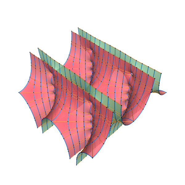
Figure 1.1. Scherk’s surface with four additional handles

Our paper is organized as follows: in the second section, we recall the background information about the Weierstrass representation, conjugate surfaces, and Teichmüller Theory, which we will need to construct our family of surfaces. In the third section, we outline our method and begin the construction by computing triples of relevant flat structures corresponding to candidate for the Weierstrass representation for the $g$-handled Scherk surfaces. In the fourth section, we define a finite dimensional moduli space $\mathcal{M}_{g}$ of such triples and define a non-negative height function $\operatorname{\mathcal{H}}:\mathcal{M}_{g}\to\mathbb{R}$ on that moduli space; a well-defined $g$-handled Scherk surface $S_{g}$ will correspond to a zero of that height function. Also in section 4, we prove that this height function is proper on $\mathcal{M}_{g}$.

In section 5, we show that the only critical points of $\operatorname{\mathcal{H}}$ on a certain locus $\mathcal{Y}_{g}\subset\mathcal{M}_{g}$ arc at $\operatorname{\mathcal{H}}^{-1}\{0\}\cap\mathcal{Y}$, proving the existence of the desired surfaces. We define this locus $\mathcal{Y}_{g}\subset\mathcal{M}_{g}$ as an extension of a desingularization of the $(g-1)$-handled Scherk surface $S_{g-1}$, viewed as an element of $\mathcal{M}_{g-1}\subset\partial\overline{\mathcal{M}_{g}}$, itself a stratum of the boundary $\partial\overline{\mathcal{M}_{g}}$ of the closure $\overline{\mathcal{M}_{g}}$ of $\mathcal{M}_{g}$.

In section 6, we show that the resulting surfaces $\{S_{g}\}$ are all embedded.

2. Background and Notation

2.1. History of doubly-periodic Minimal Surfaces

In 1835, Scherk [21] discovered a $1$-parameter family of properly embedded doubly-periodic minimal surfaces $S_{0}(\theta)$ in euclidean space. These surfaces are invariant under a lattice $\Gamma=\Gamma_{\theta}$ of horizontal euclidean translations of the plane which induce orientation-preserving isometries of the surface $S_{0}(\theta)$. If we identify the $xy$-plane with $\mathbb{C}$, this lattice is spanned by vectors $1,e^{i\theta}$.

In the upper half space, $S_{0}(\theta)$ is asymptotic to a family of equally spaced half planes. The same holds in the lower half space for a different family of half planes. The angle between these two families is the parameter $\theta\in(0,\pi/2]$. The quotient surface $S_{0}(\theta)/\Gamma_{\theta}$ is conformally equivalent to a sphere punctured at $\pm 1,\pm e^{i\theta}$.

Lazard-Holly and Meeks [15] have shown that all embedded genus 0 doubly-periodic surfaces belong to this family.

Since then, many more properly embedded doubly-periodic minimal surfaces in euclidean space have been found:

Karcher [11] and Meeks-Rosenberg [16] constructed a 3-dimensional family of genus-one examples where the bottom and top planar ends are parallel. Some of these surfaces can be visualized as a fence of Scherk towers.

Pérez, Rodriguez and Traizet [20] have shown that any doubly-periodic minimal surface of genus one with parallel ends belongs to this family.

The first attempts to add further handles to these surfaces failed, and similarly it seemed to be impossible to add just one handle to Scherk’s doubly-periodic surface between every pair of planar ends.

However, Wei [30] added another handle to Karcher’s examples (where all ends are parallel) by adding the handle between every second pair of ends. This family has been generalized by Rossman, Thayer and Wohlgemuth [26] to include more ends. Recently, Connor and Weber [3] adapted Traizet’s regeneration method to construct many examples of arbitrary genus and arbitrarily many ends.

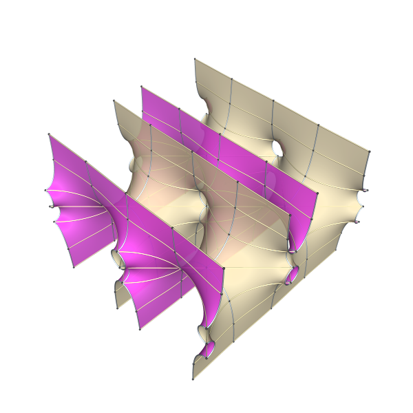
Figure 2.2. Scherk’s surface with an additional handle

Soon after Wei’s example, Karcher found an orthogonally-ended doubly-periodic Scherk-type surface with handle by also adding the handle only between every second pair of ends, see figure 2.2.

Baginski and Ramos-Batista [1] as well as Douglas [5] have shown that the Karcher example can be deformed to a 1-parameter family by changing the angle between the ends.

On the theoretical side, Meeks and Rosenberg [17] have shown the following:

Theorem 2.1.

A complete embedded minimal surface in $\mathbb{E}^{3}/\Gamma$ has only finitely many ends. In particular, it has finite topology if and only if it has finite genus.

Theorem 2.2.

A complete embedded minimal surface in $\mathbb{E}^{3}/\Gamma$ has finite total curvature if and only if it has finite topology. In this case, the surface can be given by holomorphic Weierstrass data on a compact Riemann surface with finitely many punctures which extend meromorphically to these punctures.

2.2. Weierstrass Representation

Let $S$ be a minimal surface in space with metric $ds$, and denote the underlying Riemann surface by $\mathcal{R}$. The stereographic projection of the Gauss map defines a meromorphic function $G$ on $\mathcal{R}$, and the complex extension of the third coordinate differential $dx_{3}$ defines a holomorphic 1-form $dh$ on $\mathcal{R}$, called the height differential. The data $(\mathcal{R},G,dh)$ comprise the Weierstrass data of the minimal surface. Via

$$\omega_{1} =\frac{1}{2}(G^{-1}-G)dh$$

$$\omega_{2} =\frac{i}{2}(G^{-1}+G)dh$$

$$\omega_{3} =dh$$

one can reconstruct the surface as

$$z\mapsto\operatorname{Re}\int_{\cdot}^{z}(\omega_{1},\omega_{2},\omega_{2})$$

Vice versa, this Weierstrass representation can be used on any set of Weierstrass data to define a minimal surface in space. Care has to be taken that the metric becomes complete.

This procedure works locally, but the surface is only well-defined globally if the periods

$$\operatorname{Re}\int_{\gamma}\frac{1}{2}(G^{-1}-G)dh,\frac{i}{2}(G^{-1}+G)dh,dh)$$

vanish for every cycle $\gamma\subset\mathcal{R}$. The problem of finding compatible meromorphic data $(G,dh)$ which satisfies the above conditions on the periods of $\omega_{i}$ is known as ‘the period problem for the Weierstrass representation’.

These period conditions are equivalent to

(2.1) $$\operatorname{Re}\int_{\gamma}dh=0$$

and

(2.2) $$\int_{\gamma}Gdh=\overline{\int_{\gamma}G^{-1}dh}.$$

For surfaces that are intended to be periodic, one can either define Weierstrass data on periodic surfaces, or more commonly, one can insist that equations (2.1) and (2.2) hold for only some of the cycles, with the rest of the homology having periods that generate some discrete subgroup of Euclidean translations. Our setting will be of the latter type, with periods that either vanish or are in a rank-two abelian group of orthogonal horizontal translations.

2.3. Flat Structures

The forms $\omega_{i}$ lead to singular flat structures on the underlying Riemann surfaces, defined via the line elements $ds_{\omega_{i}}=|\omega_{i}|$. These singular metrics are flat away from the support of the divisor of $\omega_{i}$; on elements $p$ of that divisor, the metrics have cone points with angles equal to $2\pi(ord_{\omega_{i}}(p)+1)$. More importantly, the periods of the forms are given by the Euclidean geometry of the developed image of the metric $ds_{\omega_{i}}$ — a period of a cycle $\gamma$ is the (complex) distance $\mathbb{C}$ between consecutive images of a distinguished point in $\gamma$. We reverse this procedure in Section 3: we use putative developed images of the one-forms $Gdh$, $G^{-1}dh$, and $dh$ to solve formally the period problem for some formal Weierstrass data. For more details about the properties of flat structures associated to meromorphic 1-forms in connection with minimal surfaces, see [27].

2.4. The Conjugate Plateau Construction and Krust’s Theorem

The material here will be needed in Section 6 where we will prove the embeddedness of our surfaces. General references for the cited theorems of this subsection are [19] and [4].

Given a minimal immersion

$$F:z\mapsto\operatorname{Re}\int^{z}\omega\quad,$$

then the immersions

$$F_{t}:z\mapsto\operatorname{Re}\int^{z}e^{it}\omega$$

define the associate family of minimal surfaces. Among them, the conjugate surface $F^{*}=F_{\pi/2}$ is of special importance because symmetry properties of $F$ correspond to symmetry properties of $F^{*}$ as follows:

Theorem 2.3.

If a minimal surface patch is bounded by a straight line, the conjugate patch is bounded by a planar symmetry curve, and vice versa. Angles at corresponding vertices are the same.

If $\ell_{1}$ and $\ell_{2}$ are a pair of intersecting straight lines on the conjugate patch corresponding to the intersection of a pair of (planar) symmetry curves lying on planes $P_{1}$ and $P_{2}$, then the lines $\ell_{1}$ and $\ell_{2}$ span a plane orthogonal to the line common to $P_{1}$ and $P_{2}$.

Proof.

The first paragraph is well-known: see [12] for example. The second paragraph is elementary, for if $P$ is a plane of reflective symmetry, then the normal to the surface must lie in the plane. At the intersection of two such planes, the normal must lie in both planes, hence in the line $L$ of intersection of the two planes. But the Gauss map is preserved by the conjugacy correspondence, hence both of the corresponding straight lines $\ell_{1}$ and $\ell_{2}$ are orthogonal to $L$. Thus the plane spanned by $\ell_{1}$ and $\ell_{2}$ is normal to $L$, the line of intersection of $P_{1}$ and $P_{2}$. ∎

The best-known example of a conjugate pair are the catenoid and one full turn of the helicoid.

The second-best-known examples are the singly- and doubly-periodic Scherk surfaces.

To get started with the conjugate Plateau construction, one can take a boundary contour bounded by straight lines and solves the Plateau problem using the classic result of Douglas and Radó (see [14] for a proof):

Theorem 2.4.

Let $\Gamma$ be a Jordan curve in $\mathbb{E}^{3}$ bounding a finite-area disk. Then there exists a continuous map $\psi$ from the closed unit disk $\bar{D}$ into $\mathbb{E}^{3}$ such that

1. $\psi$ maps $S^{1}=\partial D$ monotonically onto $\Gamma$.

2. $\psi$ is harmonic and almost conformal in $D$.

3. $\psi(\bar{D})$ minimizes the area among all admissible maps.

Here almost conformal allows a vanishing derivative and admissible maps on the disk are required to be in $H^{1,2}(D,\mathbb{E}^{3})$ so that their trace on $\partial D$ can be represented by a weakly monotonic, continuous mapping $\partial D\to\Gamma$.

For good boundary curves, one obtains the embeddedness and uniqueness of the Plateau solution for free by

Theorem 2.5.

If $\Gamma$ has a one-to-one parallel projection onto a planar convex curve, then $\Gamma$ bounds at most one disk-type minimal surface which can be expressed as the graph of a function $f:\mathbb{E}^{2}\to\mathbb{E}^{3}$.

The embeddedness of a Plateau solution sometimes implies the embeddedness of the conjugate surface. This observation is due to Krust (unpublished), see [12].

Theorem 2.6 (Krust).

If a minimal surface is a graph over a convex domain, then the conjugate piece is also a graph.

2.5. Teichmüller Theory

For $M$ a smooth surface, let Teich$(M)$ denote the Teichmüller space of all conformal structures on $M$ under the equivalence relation given by pullback by diffeomorphisms isotopic to the identity map id: $M\longrightarrow M$. Then it is well-known that Teich$(M)$ is a smooth finite-dimensional manifold if $M$ is a closed surface.

There are two spaces of tensors on a Riemann surface $\mathcal{R}$ that are important for the Teichmüller theory. The first is the space QD$(\mathcal{R})$ of holomorphic quadratic differentials, i.e., tensors which have the local form $\Phi=\varphi(z)dz^{2}$ where $\varphi(z)$ is holomorphic. The second is the space of Beltrami differentials Belt$(\mathcal{R})$, i.e., tensors which have the local form $\mu=\mu(z)d\bar{z}/dz$.

The cotangent space $T^{*}_{[\mathcal{R}]}$(Teich$(M)$) is canonically isomorphic to QD$(\mathcal{R})$, and the tangent space is given by equivalence classes of (infinitesimal) Beltrami differentials, where $\mu_{1}$ is equivalent to $\mu_{2}$ if

$$\int_{\mathcal{R}}\Phi(\mu_{1}-\mu_{2})=0\qquad\text{for every }\ \Phi\in\text{QD}(\mathcal{R}).$$

If $f:\mathbb{C}\to\mathbb{C}$ is a diffeomorphism, then the Beltrami differential associated to the pullback conformal structure is $\nu=\frac{f_{\bar{z}}}{f_{z}}\frac{d\bar{z}}{dz}$. If $f_{\epsilon}$ is a family of such diffeomorphisms with $f_{0}=id$, then the infinitesimal Beltrami differential is given by

$$\frac{d}{d\epsilon}\bigm{|}_{\epsilon=0}\nu_{f_{\epsilon}}=\left(\frac{d}{d\epsilon}\bigm{|}_{\epsilon=0}f_{\epsilon}\right)_{\bar{z}}$$

We will carry out an example of this computation in section 5.2

A holomorphic quadratic differential comes with a picture that is a useful aid to one’s intuition about it. The picture is that of a pair of transverse measured foliations, whose properties we sketch briefly (see [6] for more details).

A $C^{k}$ measured foliation on $\mathcal{R}$ with singularities $z_{1},\dots,z_{l}$ of order $k_{1},\dots,k_{l}$ (respectively) is given by an open covering $\{U_{i}\}$ of $\mathcal{R}-\{z_{1},\dots,z_{l}\}$ and open sets $V_{1},\dots,V_{l}$ around $z_{1},\dots,z_{l}$ (respectively) along with real valued $C^{k}$ functions $v_{i}$ defined on $U_{i}$ s.t.

1. $|dv_{i}|=|dv_{j}|$ on $U_{i}\cap U_{j}$

2. $|dv_{i}|=|\operatorname{Im}(z-z_{j})^{k_{j}/z}dz|$ on $U_{i}\cap V_{j}$

Evidently, the kernels $\ker dv_{i}$ define a $C^{k-1}$ line field on $\mathcal{R}$ which integrates to give a foliation $\mathcal{F}$ on $\mathcal{R}-\{z_{1},\dots,z_{l}\}$, with a $k_{j}+2$ pronged singularity at $z_{j}$. Moreover, given an arc $A\subset\mathcal{R}$, we have a well-defined measure $\mu(A)$ given by

$$\mu(A)=\int_{A}|dv|$$

where $|dv|$ is defined by $|dv|_{U_{i}}=|dv_{i}|$. An important feature that we require of this measure is its “translation invariance”. That is, suppose $A_{0}\subset\mathcal{R}$ is an arc transverse to the foliation $\mathcal{F}$, with $\partial A_{0}$ a pair of points, one on the leaf $l$ and one on the leaf $l^{\prime}$; then, if we deform $A_{0}$ to $A_{1}$ via an isotopy through arcs $A_{t}$ that maintains the transversality of the image of $A_{0}$ at every time, and also keeps the endpoints of the arcs $A_{t}$ fixed on the leaves $l$ and $l^{\prime}$, respectively, then we require that $\mu(A_{0})=\mu(A_{1})$.

Now a holomorphic quadratic differential $\Phi$ defines a measured foliation in the following way. The zeros $\Phi^{-1}(0)$ of $\Phi$ are well-defined; away from these zeros, we can choose a canonical conformal coordinate $\zeta(z)=\int^{z}\sqrt{\Phi}$ so that $\Phi=d\zeta^{2}$. The local measured foliations ($\{\operatorname{Re}\zeta=\operatorname{const}\}$, $|d\operatorname{Re}\zeta|$) then piece together to form a measured foliation known as the vertical measured foliation of $\Phi$, with the translation invariance of this measured foliation of $\Phi$ following from Cauchy’s theorem.

Work of Hubbard and Masur [9] (see also alternate proofs in [13, 7, 34], following Jenkins [10] and Strebel [22], showed that given a measured foliation $(\mathcal{F},\mu)$ and a Riemann surface $\mathcal{R}$, there is a unique holomorphic quadratic differential $\Phi_{\mu}$ on $\mathcal{R}$ so that the horizontal measured foliation of $\Phi_{\mu}$ is equivalent to $(\mathcal{F},\mu)$.

2.6. Extremal length

The extremal length $\mathrm{ext}_{\mathcal{R}}([\gamma])$ of a class of arcs $\Gamma$ on a Riemann surface $\mathcal{R}$ is defined to be the conformal invariant

$$\sup_{\rho}\frac{\ell^{2}_{\rho}(\Gamma)}{\text{Area}(\rho)}$$

where $\rho$ ranges over all conformal metrics on $\mathcal{R}$ with areas $0<\text{Area}(\rho)<\infty$ and $\ell_{\rho}(\Gamma)$ denotes the infimum of $\rho$-lengths of curves $\gamma\in\Gamma$. Here $\Gamma$ may consist of all curves freely homotopic to a given curve, a union of free homotopy classes, a family of arcs with endpoints in a pair of given boundaries, or even a more general class. Kerckhoff [13] showed that this definition of extremal lengths of curves extended naturally to a definition of extremal lengths of measured foliations.

For a class $\Gamma$ consisting of all curves freely homotopic to a single curve $\gamma\subset M$, (or more generally, a measured foliation $(\mathcal{F},\mu)$) we see that $\mathrm{ext}_{(\cdot)}(\Gamma)$ (or $\mathrm{ext}_{(\cdot)}(\mu)$) can be construed as a real-valued function $\mathrm{ext}_{(\cdot)}(\Gamma)$: Teich$(M)\longrightarrow\mathbb{R}$. Gardiner [7] showed that $\mathrm{ext}_{(\cdot)}(\mu)$ is differentiable and Gardiner and Masur [8] showed that $\mathrm{ext}_{(\cdot)}(\mu)\in C^{1}$ (Teich$(M)$). In our particular applications, the extremal length functions on our moduli spaces will be real analytic: this will be explained in Proposition 4.4.

Moreover Gardiner computed that

$$d\mathrm{ext}_{(\cdot)}(\mu)\bigm{|}_{[\mathcal{R}]}=2\Phi_{\mu}$$

so that

(2.3) $$\left(d\mathrm{ext}_{(\cdot)}(\mu)\bigm{|}_{[\mathcal{R}]}\right)[\nu]=4\operatorname{Re}\int_{\mathcal{R}}\Phi_{\mu}\nu.$$

2.7. A Brief Sketch of the Proof

In this subsection, we sketch basic logic of the approach and the ideas of the proofs, as a step-by-step recipe.

Step 1. Draw the Surface. The first step in proving the existence of a minimal surface is to work out a detailed proposal. This can either be done numerically, as in the work of (i) Thayer [23] for the Chen-Gackstatter surfaces we discussed in [28], (ii) Boix and Wohlgemuth [2, 31, 32, 33] for the low genus surfaces we treated in [29] and (iii) Figures 2.1 and 2.2 below for the present case; or it can be schematic, showing how various portions of the surface might fit together, using plausible symmetry assumptions.

Step 2. Compute the Divisors for the Forms $Gdh$ and $G^{-1}dh$. From the model that we drew in Step 1, we can compute the divisors for the Weierstrass data, which we just defined to be the Gauss map $G$ and the ’height’ form $dh$. (Note here how important it is that the Weierstrass representation is given in terms of geometrically defined quantities — for us, this gives the passage between the extrinsic geometry of the minimal surface as defined in Step 1 and the conformal geometry and Teichmüller theory of the later steps.) Thus we can also compute the divisors for the meromorphic forms $Gdh$ and $G^{-1}dh$ on the Riemann surface (so far undetermined, but assumed to exist) underlying the minimal surface. Of course the divisors for a form determine the form up to a constant, so the divisor information nearly determines the Weierstrass data for our surface. Here our schematics suggest the appropriate divisor information, and this is confirmed by the numerics.

Step 3. Compute the Flat Structures for the Forms $Gdh$ and $G^{-1}dh$ required by the period conditions. A meromorphic form on a Riemann surface defines a flat singular (conformal) metric on that surface: for example, from the form $Gdh$ on our putative Riemann surface, we determine a line element $ds_{Gdh}=|Gdh|$. This metric is locally Euclidean away from the support of the divisor of the form and has a complete Euclidean cone structure in a neighborhood of a zero or pole of the form. Thus we can develop the universal cover of the surface into the Euclidean plane.

The flat structures for the forms $Gdh$ and $G^{-1}dh$ are not completely arbitrary: because the periods for the pair of forms must be conjugate (formula 2.2), the flat structures must develop into domains which have a particular Euclidean geometric relationship to one another. This relationship is crucial to our approach, so we will dwell on it somewhat. If the map $\operatorname{dev}:\Omega\longrightarrow\mathbb{E}^{2}$ is the map which develops the flat structure of a form, say $\alpha$, on a domain $\Omega$ into $\mathbb{E}^{2}$, then the map $\operatorname{dev}$ pulls back the canonical form $dz$ on $\mathbb{C}\cong\mathbb{E}^{2}$ to the form $\alpha$ on $\omega$. Thus the periods of $\alpha$ on the Riemann surface are given by integrals of $dz$ along the developed image of paths in $\mathbb{C}$, i.e. by differences of the complex numbers representing endpoints of those paths in $\mathbb{C}$.

We construe all of this as requiring that the flat structures develop into domains that are “conjugate”: if we collect all of the differences in positions of parallel sides for the developed image of the form $Gdh$ into a large complex-valued $n$-tuple $V_{Gdh}$, and we collect all of the differences in positions of corresponding parallel sides for the developed image of the form $G^{-1}dh$ into a large complex-valued n-tuple $V_{G^{-1}dh}$, then these two complex-valued vectors $V_{Gdh}$ and $V_{G^{-1}dh}$ should be conjugate. Thus, we translate the “period problem” into a statement about the Euclidean geometry of the developed flat structures. This is done at the end of section 3.

The period problem 2.1 for the form $dh$ will be trivially solved for the surfaces we treat here.

Step 4. Define the moduli space of pairs of conjugate flat domains. Now we work backwards. We know the general form of the developed images (called $\Omega_{Gdh}$ and $\Omega_{G^{-1}dh}$, respectively) of flat structures associated to the forms $Gdh$ and $G^{-1}dh$, but in general, there are quite a few parameters of the flat structures left undetermined; this holds even after we have assumed symmetries, determined the Weierstrass divisor data for the models and used the period conditions 2.2 to restrict the relative Euclidean geometries of the pair $\Omega_{Gdh}$ and $\Omega_{G^{-1}dh}$. Thus, there is a moduli space $\Delta$ of possible candidates of pairs $\Omega_{Gdh}$ and $\Omega_{G^{-1}dh}$: our period problem (condition 2.2) is now a conformal problem of finding such a pair which are conformally equivalent by a map which preserves the corresponding cone points. (Solving this problem means that there is a well-defined Riemann surface which can be developed into $\mathbb{E}^{2}$ in two ways, so that the pair of pullbacks of the form $dz$ give forms $Gdh$ and $G^{-1}dh$ with conjugate periods.)

The condition of conjugacy of the domains $\Omega_{Gdh}$ and $\Omega_{G^{-1}dh}$ often dictates some restrictions on the moduli space, and even a collection of geometrically defined coordinates. We work these out in section 3.

Step 5. Solve the Conformal Problem using Teichmüller theory. At this juncture, our minimal surface problem has become a problem in finding a special point in a product of moduli spaces of complex domains: we will have no further references to minimal surface theory. The plan is straightforward: we will define a height function $\operatorname{\mathcal{H}}:\Delta\longrightarrow\mathbb{R}$ with the properties:

1. (Reflexivity) The height $\operatorname{\mathcal{H}}$ equals $0$ only at a solution to the conformal problem

2. (Properness) The height $\operatorname{\mathcal{H}}$ is proper on $\Delta$. This ensures the existence of a critical point.

3. (Non-degenerate Flow) If the height $\operatorname{\mathcal{H}}$ at a pair $(\Omega_{Gdh},\Omega_{G^{-1}dh})$ does not vanish, then the height $\operatorname{\mathcal{H}}$ is not critical at that pair $(\Omega_{Gdh},\Omega_{G^{-1}dh})$.

This is clearly enough to solve the problem: we now sketch the proofs of these steps.

Step 5a. Reflexivity. We need conformal invariants of a domain that provide a complete set of invariants for Reflexivity, have estimable asymptotics for Properness, and computable first derivatives (in moduli space) for the Non-degenerate Flow property. One obvious choice is a set of functions of extremal lengths for a good choice of curve systems, say $\Gamma=\{\gamma_{1},\dots,\gamma_{g}\}$ on the domains. These are defined for our examples in section 4.1. We then define a height function $\operatorname{\mathcal{H}}$ which vanishes only when there is agreement between all of the extremal lengths $\mathrm{ext}_{\Omega_{Gdh}}(\gamma_{i})=\mathrm{ext}_{\Omega_{G^{-1}dh}}(\gamma_{i})$ and which blows up when $\mathrm{ext}_{\Omega_{Gdh}}(\gamma_{i})$ and $\mathrm{ext}_{\Omega_{G^{-1}dh}}(\gamma_{i})$ either decay or blow up at different rates. See for example Definition 4.2 and Lemma 4.11.

Step 5b Properness. Our height function will measure differences in the extremal lengths $\mathrm{ext}_{\Omega_{Gdh}}(\gamma_{i})$ and $\mathrm{ext}_{\Omega_{G^{-1}dh}}(\gamma_{i})$. A geometric degeneration of the flat structure of either $\Omega_{Gdh}$ or $\Omega_{G^{-1}dh}$ will force one of the extremal lengths $\mathrm{ext}_{\bullet}(\gamma_{i})$ to tend to zero or infinity, while the other extremal length stays finite and bounded away from zero. This is a straightforward situation where it will be obvious that the height function will blow up. A more subtle case arises when a geometric degeneration of the flat structure forces both of the extremal lengths $\mathrm{ext}_{\Omega_{Gdh}}(\gamma_{i})$ and $\mathrm{ext}_{\Omega_{G^{-1}dh}}(\gamma_{i})$ to simultaneously decay (or explode). In that case, we begin by observing that there is a natural map between the vector $<\mathrm{ext}_{\Omega_{Gdh}}(\gamma_{i})>$ and the vector $<\mathrm{ext}_{\Omega_{G^{-1}dh}}(\gamma_{i})>$. This pair of vectors is reminiscent of pairs of solutions to a hypergeometric equation, and we show, by a monodromy argument analogous to that used in the study of those equations, that it is not possible for corresponding components of that vector to vanish or blow up at identical rates. In particular, we show that the logarithmic terms in the asymptotic expansion of the extremal lengths near zero have a different sign, and this sign difference forces a difference in the rates of decay that is detected by the height function, forcing it to blow up in this case. The monodromy argument is given in section 4.3, and the properness discussion consumes section 4.2.

Step 5c. Non-degenerate Flow. The domains $\Omega_{Gdh}$ and $\Omega_{G^{-1}dh}$ have a remarkable property: if $\mathrm{ext}_{\Omega_{Gdh}}(\gamma_{i})>\mathrm{ext}_{\Omega_{G^{-1}dh}}(\gamma_{i})$, then when we deform $\Omega_{Gdh}$ so as to decrease $\mathrm{ext}_{\Omega_{Gdh}}(\gamma_{i})$, the conjugacy condition forces us to deform $\Omega_{G^{-1}dh}$ so as to increase $\mathrm{ext}_{\Omega_{G^{-1}dh}}(\gamma_{i})$. We can thus always deform $\Omega_{Gdh}$ and $\Omega_{G^{-1}dh}$ so as to reduce one term of the height function $\operatorname{\mathcal{H}}$. We develop this step in Section 5.

Step 5d. Regeneration. In the process described in the previous step, an issue arises: we might be able to reduce one term of the height function via a deformation, but this might affect the other terms, so as to not provide an overall decrease in height. We thus seek a locus $\mathcal{Y}$ in our moduli space where the height function has but a single non-vanishing term, and all the other terms vanish to at least second order. If we can find such a locus $\mathcal{Y}$, we can flow along that locus to a solution. To begin our search for such a locus, we observe which flat domains arise as limits of our domains $\Omega_{Gdh}$ and $\Omega_{G^{-1}dh}$: commonly, the degenerate domains are the flat domains for a similar minimal surface problem, maybe of slightly lower genus or fewer ends.

We find our desired locus by considering the boundary of the (closure) of the moduli space $\Delta$: this boundary has strata of moduli spaces $\Delta^{\prime}$ for minimal surface problems of lower complexity. By induction, there are solutions of those problems represented on such a boundary strata $\Delta^{\prime}$ (with all of the corresponding extremal lengths in agreement), and we prove that there is a nearby locus $\mathcal{Y}$ inside the larger moduli space $\Delta$ which has the analogues of those same extremal lengths in agreement. As a corollary of that condition, the height function on $\mathcal{Y}$ has the desired simple properties.

2.8. The Geometry of Orthodisks

In this section we introduce the notion of orthodisks.

Consider the upper half plane $\mathbb{H}$ and $n\geq 3$ distinguished points $t_{i}$ on the real line. The point $t_{\infty}=\infty$ will also be a distinguished point. We will refer to the upper half plane together with these data as a conformal polygon and to the distinguished points as vertices. Two conformal polygons are conformally equivalent if there is a biholomorphic map between the disks carrying vertices to vertices, and fixing $\infty$.

Let $a_{i}$ be some odd integers such that

(2.4) $$a_{\infty}=-4-\sum_{i}a_{i}$$

By a Schwarz-Christoffel map we mean the map

(2.5) $$F:z\mapsto\int_{i}^{z}(t-t_{1})^{a_{1}/2}\cdot\ldots\cdot(t-t_{n})^{a_{n}/2}dt$$

A point $t_{i}$ with $a_{i}>-2$ is called finite, otherwise infinite. By Equation 2.4, there is at least one finite vertex.

Definition 2.7.

Let $a_{i}$ be odd integers. The pull-back of the flat metric on $\mathbb{C}$ by $F$ defines a complete flat metric with boundary on $\mathbb{H}\cup\mathbb{R}$ without the infinite vertices. We call such a metric an orthodisk. The $a_{i}$ are called the vertex data of the orthodisk. The edges of an orthodisk are the boundary segments between vertices; they come in a natural order. Consecutive edges meet orthogonally at the finite vertices. Every other edge is parallel under the parallelism induced by the flat metric of the orthodisk. Oriented distances between parallel edges are called periods. We will discuss the relationship of these periods to the periods arising in the minimal surface context in Section 3.

The periods can have $4$ different signs: $+1,-1,+i,-i$.

The interplay between these signs is crucial to our monodromy argument, especially Lemma 4.11.

Remark 2.8.

The integer $a_{i}$ corresponds to an angle $(a_{i}+2)\pi/2$ of the orthodisk. Negative angles are meaningful because a vertex (with a negative angle $-\theta$) lies at infinity and is the intersection of a pair of lines which also intersect at a finite point, where they make a positive angle of $+\theta$.

In all the drawings of the orthodisks to follow, we mean the domain to be to the left of the boundary, where we orient the boundary by the order of the points $t_{i}$.

2.9. Scherk’s and Karcher’s Doubly-Periodic Surfaces

The singly- and doubly-periodic Scherk surfaces are conjugate spherical minimal surfaces whose Weierstrass data lead to no computational difficulties and whose orthodisk description illustrates the basic concepts in an ideal way.

We discuss first the Weierstrass representation of the doubly-periodic Scherk surfaces $S_{0}(\theta)$ (see figure 2.1).

$$G(z)=z$$

and

$$dh=z^{-1}\frac{idz}{z^{2}+z^{-2}-2\cos{2\phi}}$$

on the Riemann sphere punctured at the four points $q=\pm e^{\pm i\phi}$.

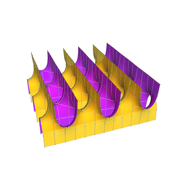
Figure 2.1. Scherk’s surface

The residues of $dh$ at the punctures have the real values $\frac{\pm 1}{4\sin{2\phi}}$ and hence we have no vertical periods. At the punctures (which correspond to the ends) the Gauss map is horizontal and takes the values $\pm e^{\pm i\phi}$ so that the angle between two ends is $2\phi$. Because of this, the horizontal surface periods around a puncture $q$ are given as complex numbers by

$$\operatorname{Re} \oint_{q}\frac{i}{2}\left(G+\frac{1}{G}\right)dh+i\operatorname{Re}\oint_{q}\frac{1}{2}\left(\frac{1}{G}-G\right)dh=$$

$$=\operatorname{Re}\left(\pi i^{2}\left(G(q)+\overline{G(q)}\right)\operatorname{Res}_{q}dh\right)-i\operatorname{Re}\left(\pi i\left(G(q)-\overline{G(q)}\right)\operatorname{Res}_{q}dh\right)$$

$$=-2\pi\overline{G(q)}\operatorname{Res}_{q}dh.$$

These numbers span a horizontal lattice in $\mathbb{C}$ so that the surface is indeed doubly-periodic. Indeed we can now regard the result as being defined over the even squares of a sheared checkerboard with vertices given by the period lattice.

Our principal interest in this paper will be with handle addition for the orthogonal Scherk surface $S_{0}=S_{(}\pi/2)$, i.e the case where in the above we set $\phi=\pi/2$ to obtain a period lattice which is a multiple of the Gaussian integers.

It would be interesting to shear these surfaces, as in the work of Ramos-Batista-Baginsky [1] or Douglas [5], so that the periods span a non-orthogonal horizontal lattice, or to add handles to a sheared surface $S_{1}(\theta)$.

The construction of $S_{1}$ is due to Hermann Karcher [11] who found a way to ‘add a handle’ to the classical Scherk surface. Here we mean that he found a doubly-periodic minimal surface whose fundamental domain is equivariantly isotopic to a doubly-periodic surface formed by adding a handle to the Scherk surface above.

We now reprove the result of Karcher from the perspective of orthodisks.

The quotient surface of $S_{1}$ by its horizontal period lattice is a square torus with four punctures corresponding to the ends. We will construct this surface using the Weierstrass data given by figure 2.3 below. We begin with the figure on the far right. The points with labels $1$ to $4$ are 2-division points on the torus and correspond to the points with vertical normal on $S_{1}$. The points $E_{1},E_{2}$ and their symmetric counterparts (not labelled) correspond to the ends. The point $E_{1}$ is placed on the straight segment between $1$ and $2$, and its position is a free parameter that will be used to solve the period problem. The other poles are then determined by the reflective symmetries of the square.

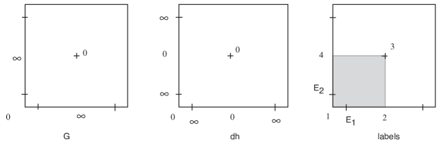
Figure 2.3. Divisors for the doubly-periodic Scherk surface with handle

We obtain the domains $|Gdh|$ and $|\frac{1}{G}dh|$ by developing just the shaded square the regions given by figure 2.3.

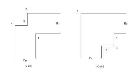
Figure 2.4. $|Gdh|$ and $|\frac{1}{G}dh|$ orthodisks of a quarter piece

As usual, the domains lie in separate planes and the half-strips extend to infinity.

Observe that these domains are arranged to be symmetric with respect to the $y=-x$ diagonal.

Remark 2.9.

Four copies of the (say) $|Gdh|$ domain fit together to form a region as in Figure 2.5 with orthogonal half-strips, where a square from the center has removed. This square (with opposite edges identified) corresponds precisely to the added handle.

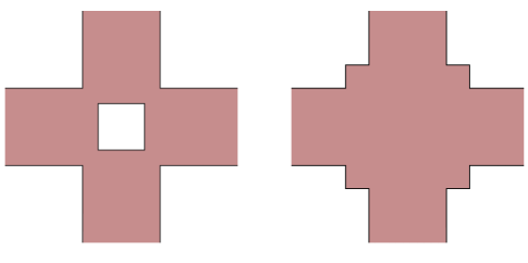
Figure 2.5. $|Gdh|$ and $|\frac{1}{G}dh|$ orthodisks of a fundamental domain

The period condition requires $Gdh$ and $\frac{1}{G}dh$ to have the same residues at $E_{1}$ and $E_{2}$ (so that the half-infinite strips need to have the same width) and the remaining periods need to be complex conjugate so that the $23$ and $34$ edges need to have the same length in both domains.

This is a one-dimensional period problem, and as is often the case, one can solve it via an intermediate value argument. There are two versions of this argument, one approaching the problem from the perspective of the period integrals on a fixed Riemann surface, and the other from the perspective of the conformal moduli of the pair of orthodisks. We begin with the version based on the behavior of the period integrals in the limit cases. We keep the discussion as close as possible to the orthodisk description by using Schwarz-Christoffel maps from the upper half plane to parametrize the domains for $Gdh$ and $\frac{1}{G}$:

$$f_{Gdh}:z \mapsto\int^{z}{\frac{{\sqrt{r}}\,{\sqrt{-1+{x^{2}}}}}{{\sqrt{-1+{r^{2}}}}\,{\sqrt{x}}\,\left(-{r^{2}}+{x^{2}}\right)}}dx$$

$$f_{1/Gdh}:z \mapsto\int^{z}{\frac{{\sqrt{-1+{r^{2}}}}\,{\sqrt{x}}}{{\sqrt{r}}\,{\sqrt{-1+{x^{2}}}}\,\left(-{r^{2}}+{x^{2}}\right)}}dx$$

Here the point $-1<-r<0<r<1<\infty$ on the real axis are mapped to the labels $4,E_{2},1,E_{1},2,3$, respectively. The normalization is choosen so that

$$\operatorname{Res}_{r}Gdh=\frac{1}{2r}=\operatorname{Res}_{r}\frac{1}{G}dh$$

The parameter $r$ determines the relative position of $E_{1}$ and will now be determined. For this we compute the lengths of the edge $23$ as functions of $r$ using hypergeometric functions as follows:

$$A_{Gdh} = \int_{1}^{\infty}\frac{1}{G}dh = \sqrt{\pi}\frac{\sqrt{r}}{\sqrt{1-r^{2}}}\frac{\Gamma(5/4)}{\Gamma(7/4)}F\left(\frac{1}{4},1,\frac{7}{4},r^{2}\right)$$

$$A_{1/Gdh} = \int_{1}^{\infty}Gdh = 2\sqrt{\pi}\frac{\sqrt{1-r^{2}}}{\sqrt{r}}\frac{\Gamma(3/4)}{\Gamma(1/4)}F\left(\frac{3}{4},1,\frac{5}{4},r^{2}\right)$$

The period condition requires

$$A_{Gdh}(r)=A_{1/Gdh}(r)\ .$$

To determine $r$, notice the ‘boundary conditions’

$$A_{Gdh}(0) =\infty$$

$$A_{1/Gdh}(0) =0$$

$$A_{Gdh}(1) =\frac{\pi}{2}$$

$$A_{1/Gdh}(1) =\infty$$

so that the intermediate value theorem implies the existence of a solution.

Alternatively, we can give an intermediate value theorem argument based on extremal length. This is more in keeping with our theme of converting the period problem for minimal surfaces into a conformal problem for orthodisks.

In terms of the orthodisks, the family of possible pairs $\{\Omega_{Gdh},\Omega_{G^{-1}dh}\}$ of orthodisks can be normalized so that each half-strip end of either $\Omega_{Gdh}$ or $\Omega_{G^{-1}dh}$ has width one. Then the family of pairs $\{\Omega_{Gdh},\Omega_{G^{-1}dh}\}$ is parametrized by the distance, say $d_{13}$, between the points $1$ and $3$ in the domain $\Omega_{Gdh}$: there is degeneration in the domain $\Omega_{Gdh}$ as $d_{13}\longrightarrow 0$, and there is degeneration in the other domain $\Omega_{G^{-1}dh}$ as $d_{13}\longrightarrow 2\sqrt{2}$.

Consider the family $\mathcal{F}$ of curves connecting the side $\overline{E_{1}2}$ with the side $\overline{E_{2}4}$. Let us examine the extremal length of this family under the pair of limits. In the first case, as $d_{13}\longrightarrow 0$, the two edges $\overline{E_{2}4}$ and $\overline{E_{1}2}$ are becoming disconnected in $\Omega_{Gdh}$, while the domain $\Omega_{G^{-1}dh}$ is converging to a non-degenerate domain. Thus the extremal length of $\mathcal{F}$ in $\Omega_{Gdh}$ is becoming infinite, while the corresponding extremal length in $\Omega_{G^{-1}dh}$ is remaining finite and positive. The upshot is that near this limit point, $\mathrm{ext}_{\Omega_{Gdh}}(\mathcal{F})>\mathrm{ext}_{\Omega_{G^{-1}dh}}(\mathcal{F})$.

Near the other endpoint, where $d_{13}$ is nearly $\sqrt{2}$ in $\Omega_{Gdh}$, the opposite inequality holds. This claim is a bit more subtle, as since the pair of segments $\overline{23}$ and $\overline{34}$ are converging to a single point, we see both extremal lengths $\mathrm{ext}_{\Omega_{Gdh}}(\mathcal{F})$ and $\mathrm{ext}_{\Omega_{G^{-1}dh}}(\mathcal{F})$ are tending to zero. Yet it is quite easy to compute that the rates of vanishing are quite different, yielding $\mathrm{ext}_{\Omega_{Gdh}}(\mathcal{F})<\mathrm{ext}_{\Omega_{G^{-1}dh}}(\mathcal{F})$ near this endpoint. To see this let $\Omega_{Gdh}(\epsilon)$ and $\Omega_{G^{-1}dh}(\epsilon)$ denote the domains $\Omega_{Gdh}$ (and $\Omega_{G^{-1}dh}$, respectively) with the lengths of sides $\overline{23}$ or $\overline{34}$ being $\epsilon$. We are interested in the Schwarz-Christoffel maps $F_{Gdh,\epsilon}:\mathbb{H}\to\Omega_{Gdh}(\epsilon)$ and $F_{1/Gdh,\epsilon}:\mathbb{H}\to\Omega_{G^{-1}dh}(\epsilon)$, and in particular at the preimages $x_{2}(\epsilon)$, $x_{3}(\epsilon)$, $x_{4}(\epsilon)$ (and $y_{2}(\epsilon)$, $y_{3}(\epsilon)$, $y_{4}(\epsilon)$, resp. ) under $F_{Gdh,\epsilon}$ (and $F_{1/Gdh}(\epsilon)$, resp.) of the vertices marked $2$, $3$ and $4$. It is straighforward to see that up to a factor that is bounded away from both $0$ and $\infty$ as $\epsilon\to 0$, these positions are given by the positions of the corresponding pre-images of the simplified (and symmetric) maps

$$F_{Gdh,\epsilon}(z)=\int^{z}t^{-1}(t-x_{2})^{-1/2}(t-x_{3})^{1/2}(t-x_{4})^{-1/2}dt$$

and

$$F_{1/Gdh,\epsilon}=\int^{z}t^{-1}(t-y_{2})^{1/2}(t-y_{3})^{-1/2}(t-y_{4})^{1/2}dt$$

where $\{x_{i}\}$ and $\{y_{i}\}$ are bounded away from zero and we have suppressed the dependence on $\epsilon$ in the expressions for the vertices. (We can ignore the factor because we can, for example, normalize the positions of the points so the the distance $x_{4}-x_{3}$ is the only free parameter. Once that is done, the factor is determined by an integral of a path beginning in the interval $[x_{4},E_{2}]$ to a point in the interval $[x_{1},E_{1}]$; in this situation, both the length of the path and the integrand are bounded away from both zero and infinity, proving the assertion.) Thus we may compute the asymptotics by setting

$$\epsilon =\int^{x_{4}}_{x_{3}}\frac{1}{t}\sqrt{\frac{t-x_{3}}{(t-x_{2})(t-x_{4})}}dt$$

$$\asymp(x_{4}-x_{3})^{1/2}\int^{1}_{0}\sqrt{\frac{s}{(s+1)(s-1)}}ds$$

using that $s=\frac{t-x_{3}}{x_{4}-x_{3}}$, that we have bounded $X_{2},x_{3},x_{4}$ away from zero, and that we have assumed the symmetry $x_{4}-x_{3}=x_{3}-x_{2}$.

Thus $x_{4}(\epsilon)-x_{3}(\epsilon)=0(\epsilon^{2})$.

A similar formal substitution into the integral expression for $F_{1/Gdh}(\epsilon)$, again using the symmetry of the domain, yields that

$$\epsilon =\int^{y_{4}}_{y_{3}}\frac{1}{t}\sqrt{\frac{(t-y_{2})(t-y_{4})}{(t-y_{3})}}dt$$

$$\asymp(y_{4}-y_{3})^{3/2}\int^{1}_{0}\sqrt{\frac{(s-1)(s+1)}{s}}ds$$

so $(y_{4}-y_{3})=0(\epsilon^{2/3})$.

As the extremal length $\mathrm{ext}_{\Omega_{Gdh}}(\mathcal{F})$ and $\mathrm{ext}_{\Omega_{G^{-1}dh}}(\mathcal{F})$ of $\mathcal{F}$ are given by the extremal lengths in $\mathbb{H}$ for a family of arcs between intervals that surround $x_{2}$, $x_{3}$, and $x_{4}$ (or $y_{2}$, $y_{3}$, and $y_{4}$) in $\mathbb{H}$, and those extremal lengths are monotone increasing in the length of the excluded interval $\overline{x_{2}x_{4}}$ (or $\overline{y_{2}y_{4}}$, we see from the displayed formulae above and that $\epsilon^{2/3}>\epsilon^{2}$ for $\epsilon$ small implies that

(2.6) $$\mathrm{ext}_{\Omega_{Gdh}}(\mathcal{F})<\mathrm{ext}_{\Omega_{G^{-1}dh}}(\mathcal{F})$$

for $\epsilon$ small, as desired.

3. Orthodisks for the Scherk family

In this section, we begin our proof of the existence of the surfaces $S_{g}$, the doubly-periodic Scherk surfaces with $g$ handles. We begin by deciding on the form of the relevant orthodisks; our plan is to adduce these orthodisks from the orthodisks for the classical Scherk surface $S_{0}$ and the Karcher surface $S_{1}$. It will then turn out that these orthodisks are quite similar to the orthodisks we used in [28] to prove the existence of the surfaces $E_{g}$ of genus $g$ with one Enneper-like end.

In this section we will introduce pairs of orthodisks and outline the existence proof for the $S_{g}$ surfaces, using the $E_{g}$ surfaces as the model case.

The existence proof consists of several steps. The first is to set up a space $\Delta=\Delta_{g}$ of geometric coordinates such that each point in this space gives rise to a pair of conjugate orthodisks as described in section 2.

Given such a pair, one canonically obtains a pair of marked Riemann surfaces with meromorphic $1$-forms having complex conjugate periods. If the surfaces were conformally equivalent, these two $1$-forms would serve as the $1$-forms $Gdh$ and $\frac{1}{G}dh$ in the Weierstrass representation.

After that, it remains to find a point in the geometric coordinate space so that the two surfaces are indeed conformal. To achieve this, a nonnegative height function $\operatorname{\mathcal{H}}$ is constructed on the coordinate space with the following properties:

1. $\operatorname{\mathcal{H}}$ is proper;

2. $\operatorname{\mathcal{H}}=0$ implies that the two surfaces are conformal;

3. Given a surface $S_{g-1}$, there is a smooth locus $\mathcal{Y}$ which lies properly in the $S_{g}$ coordinate space $\Delta_{g}$ whose closure contains $S_{g-1}\in\partial\overline{\Delta_{g}}$. On that locus $\mathcal{Y}\subset\Delta_{g}$, if $d\operatorname{\mathcal{H}}=0$, then actually $\operatorname{\mathcal{H}}=0$.

The height should be considered as some adapted measurement of the conformal distance between the two surfaces. Hence it is natural to construct such a function using conformal invariants. We have chosen to build an expression using the extremal lengths of suitable cycles.

The first condition on the height poses a severe restriction on the choice of the geometric coordinate system: The extremal length of a cycle becomes zero or infinite only if the surface develops a node near that cycle. Hence we must at least ensure that when reaching the boundary $\partial\overline{\Delta_{g}}$ of the geometric coordinate domain $\Delta_{g}$, at least one of the two surfaces degenerates conformally.

This condition is called completeness of the geometric coordinate domain $\Delta_{g}$.

Fortunately, we can use the definition of the geometric coordinates for $E_{g}$ to derive complete geometric coordinates for $S_{g}$.

We recall the geometric coordinates that we used in [28] to prove the existence of the Enneper-ended surfaces $E_{g}$. There, both domains $\Omega_{Gdh}$ and $\Omega_{G^{-1}dh}$ were bounded by staircase-like objects we referred to as ’zigzags’: in particular, the boundary of a domain was a properly embedded arc, which alternated between ($g+1$) purely vertical segments and ($g+1$) purely horizontal segments and was symmetric across a diagonal line. Any such boundary is determined up to translation by the lengths of its initial $g$ finite-length sides, and up to homothety by any subset of those of size $g-1$. Thus, the geometric coordinates we used for such a domain $\Omega_{Gdh}$ or $\Omega_{G^{-1}dh}$ were the lengths of the first $g-1$ sides. These coordinates are obviously complete.

Remark 3.1.

We were fortunate in [28], as we will be in the present case, to be able to restrict our attention to orthodisks which embed in the plane. For orthodisk systems that branch over the plane (see [29]) or are not planar (see [5]), the description of the geometric coordinates can be quite subtle.

Recall that the orthodisks for the Chen-Gackstatter surfaces of higher genus were obtained by taking the negative $y$-axis and the positive $x$-axis and replacing the subarc from $(0,-a)$ to $(a,0)$ by a monotone arc consisting of horizontal and vertical segments which were symmetric with respect to the diagonal $y=-x$. The two regions separated by this ‘zigzag’ constituted a pair of orthodisks. The geometric coordinates were given by the edge lengths of the finite segments above the diagonal $y=-x$.

For our new surfaces, we continue the above construction as follows. Denote the vertex of the new subarc that meets the diagonal by $(c,-c)$. Choose $b>c$. We then intersect the upper left region with the half planes $\{x>-b\}$ and $\{y<b\}$. Similarly, we intersect the lower right region with the half planes $\{x<b\}$ and $\{y>-b\}$. This procedure defines two domains which we denote by $\Omega_{Gdh}$ and $\Omega_{G^{-1}dh}$. We use the convention that $\Omega_{Gdh}$ is the domain where the vertex $(c,-c)$ makes a $3\pi/2$ angle.

As geometric coordinates for this pair of orthodisks we take the edge lengths as before and in addition the width $b$ of the half-infinite vertical and horizontal strips.

Theorem 3.2.

This coordinate system for $S_{g}$ is complete.

Proof.

Certainly if one of the finite edges degenerates, the conformal structure also leaves all compact sets in its moduli space. Next, if the geometric coordinate $b-c$ tends to 0, the two vertices on the diagonal $y=-x$ coalesce, so that the extremal length of the arc connecting $P_{0}E_{2}$ to $E_{1}P_{2g}$ tends to $\infty$, and so the surface has also degenerated. ∎

Why should such an orthodisk system correspond to a doubly-periodic minimal surface of genus $g$? Here we are both generalizing the intuition given by Karcher’s surface, or alternatively relying on numerical simulation (see Figure 1.1). Either way, we can conjecture the divisor data for a fundamental (and planar) piece of the surface $S_{g}$, and use this to define the orthodisk of the surface, hence the developed image of a fundamental piece.

To formalize the discussion, we introduce:

Definition 3.3.

A pair of orthodisks is called reflexive if there is a vertex- and label-preserving holomorphic map between them.

Then we have:

Theorem 3.4.

Given a reflexive pair of orthodisks of genus $g$, there is a doubly-periodic minimal surface of genus $g$ in $T\times\mathbb{E}$ with two orthogonal top and two bottom ends.

Proof.

We first construct the underlying Riemann surface by taking the $\Omega_{Gdh}$ orthodisk, doubling it along the boundary, and then taking a double branched cover of that, branched at the vertices. This gives us a Riemann surface $X_{g}$ of genus $g$.

That Riemann surface carries a natural cone metric induced by the flat metric of $\Omega_{Gdh}$. As all identifications are done by parallel translations, this cone metric has trivial holonomy and hence the exterior derivative of its developing map defines a $1$-form which we call $Gdh$. This $1$-form is well-defined, up to multiplication by a complex number.

By the reflexitivity condition, the very same Riemann surface $X_{g}$ carries another cone metric, being induced from the $\Omega_{G^{-1}dh}$ orthodisk and the canonical identification of the $\Omega_{Gdh}$ and $\Omega_{G^{-1}dh}$ orthodisks by a vertex-preserving conformal diffeomorphism. This second orthodisk defines a second $1$-form, denoted by $\frac{1}{G}dh$, also well-defined only up to scaling.

The free scaling parameters are now fixed (up to an arbitrary real scale factor which only affects the size of the surface in $\mathbb{E}^{3}$) so that the developed $\Omega_{Gdh}$ and $\Omega_{G^{-1}dh}$ are truly complex conjugate if we use the same base point and base direction for the two developing maps.

This way we have defined the Weierstrass data $G$ and $dh$ on a Riemann surface $X_{g}$.

We show next that the resulting minimal surface has the desired geometric properties. The cone points on $X_{g}$ come only from the orthodisk vertices: the finite vertices $P_{j}$, being branch points, lift to a single cone point (also denoted $P_{j}$). The other finite cone points $V_{+}$ and $V_{-}$ give also only one cone point on the surface, denoted by $V$. The half strips lead to four cone points $E_{i}$. From the cone angles we can easily deduce the divisors of the induced $1$-forms as

$$(Gdh) =P_{0}^{2}P_{2}^{2}\cdots P_{2g}^{2}E_{1}^{-1}E_{2}^{-1}E_{3}^{-1}E_{4}^{-1}$$

$$(\frac{1}{G}dh) =P_{1}^{2}P_{3}^{2}\cdots P_{2g-1}^{2}V^{2}E_{1}^{-1}E_{2}^{-1}E_{3}^{-1}E_{4}^{-1}$$

$$(dh) =P_{0}\cdots P_{2g}VE_{1}^{-1}E_{2}^{-1}E_{3}^{-1}E_{4}^{-1}$$

These data guarantee that the surface is properly immersed, without singularities, and complete. The points $P_{i}$ and $V$ correspond to the points with vertical normal at the attached handles, while the $E_{i}$ correspond to the four ends.

As $dh$ has only simple zeroes and poles, its periods will all have the same phase, and using a local coordinate it is easy to see that the periods must all be real.

For the cycles in $\Omega_{Gdh}$ and $\Omega_{G^{-1}dh}$ corresponding to finite edges, the conjugacy condition ensures that all of the periods are purely real. The cycles around the ends are similarly conjugate by the construction of the orthodisks. The symmetry of the domain ensures that the ends are orthogonal.

∎

4. Existence Proof: The Height Function

4.1. Definition and Reflexivity of the Height Function

For a cycle $c$ connecting pairs of edges denote by $\mathrm{ext}_{\Omega_{Gdh}}(c)$ and $\mathrm{ext}_{\Omega_{G^{-1}dh}}(c)$ the extremal lengths of the cycle in the $Gdh$ and $\frac{1}{G}dh$ orthodisks, respectively. Recall that this makes sense as we have a natural topological identification of these domains (up to homotopy) mapping corresponding vertices onto each other.

The height function on the space of geometric coordinates will be a sum over several summands of the following type:

Definition 4.1.

Let $c$ be a cycle. Define

$$\operatorname{\mathcal{H}}(c)=\Big{|}e^{1/\mathrm{ext}_{\Omega_{Gdh}}(c)}-e^{1/\mathrm{ext}_{\Omega_{G^{-1}dh}}(c)}\Big{|}^{2}+\Big{|}e^{\mathrm{ext}_{\Omega_{Gdh}}(c)}-e^{\mathrm{ext}_{\Omega_{G^{-1}dh}}(c)}\Big{|}^{2}$$

The rather complicated shape of this expression is required to prove the properness of the height function: Because there are sequences of points in the space of geometric coordinates which converge to the boundary so that both orthodisks degenerate for the same cycles, the above expression must be very sensitive to different rates with which this happens.

Due to the Monodromy Theorem 4.6, it is sometimes possible to detect such rate differences in the growth of $\exp\frac{1}{\mathrm{ext}(c)}$ for degenerating cycles with $\mathrm{ext}(c)\to 0$.

The assumptions of the Monodromy Theorem impose certain restrictions on the choice of cycles for the height, and there are further restrictions coming from the Regeneration Lemma 5.1 below.

Before we introduce the cycles formally, we need to set some notation. In the figure below, we have labelled the finite vertices of the staircase for $S_{g}$ as $\{P_{0},\dots,P_{2g}\}$, the end vertices as $E_{1}$ and $E_{2}$, and the finite vertices on the outside boundary components of $\Omega_{Gdh}$ and $\Omega_{G^{-1}dh}$ as $V_{+}$ and $V_{-}$, respectively. Note that in the combined Figure 4.1, the vertices $P_{i}$ proceed in a different order for the domain $\Omega_{G^{-1}dh}$ than they do for the domain $\Omega_{Gdh}$.

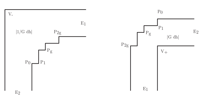
Figure 4.1. Geometric Coordinates

At this point, there is a difficulty in keeping the notation consistent; a consistent choice of orientation of the Gauss map $G$ results in the two regions switching labels as we increase the genus by one; we will circumvent that notational issue by requiring the Gauss map $G$ to have the orientation for odd genus opposite to that which is has for even genus – thus, the angle at $P_{g}$ in $\Omega_{Gdh}$ will always be $3\pi/2$, independently of $g$. See Figure 4.1.

Now let’s introduce the cycles formally.

Let $c_{i}$ denote the cycle in a domain which encircles the segment $\overline{P_{i-1}P_{i}}$; here $i$ ranges from $1$ to $g-1$, and from $g+2$ to $2g$. In addition, let $\delta$ connect the segment $\overline{E_{2}P_{0}}$ to the segment $\overline{P_{2g}E_{1}}$. This last segment $\delta$ is loosely analogous in its design and purpose to the arc we used in the second proof of the existence of the Karcher surface $S_{1}$.

We group these cycles in pairs symmetric with respect to the $y=-x$ diagonal and also require that the cycles are symmetric themselves:

To this end, set

$$\gamma_{i}=c_{i}+c_{2g+1-i},\qquad i=1,\dots,g-1.$$

These cycles will detect degeneracies on the boundary with many finite vertices, while $\delta$ detects degeneration of the pair of boundaries in $\Omega_{Gdh}$.

We next use these cycles to define a proper height function on the moduli space $\Delta_{g}$ of pairs of orthodisks. Note that $\dim\Delta_{g}=g$, so we are using $g$ cycles.

Definition 4.2.

The height for the $E_{g}$ surface is defined as

$$\operatorname{\mathcal{H}}=\sum_{i=1}^{g-1}\operatorname{\mathcal{H}}(\gamma_{i})+\operatorname{\mathcal{H}}(\delta)$$

Lemma 4.3.

If $\operatorname{\mathcal{H}}=0$, the two orthodisks are reflexive, i.e. there is a vertex preserving conformal map between them.

Proof.

Map the $\Omega_{Gdh}$ orthodisk conformally to the upper half plane $\mathbb{H}$ so that $P_{g}$ is mapped to $0$, and $V_{+}$ to $\infty$. As the domain $\Omega_{Gdh}$ is symmetric about a diagonal line connecting $P_{g}$ with $V_{+}$, our mapping is equivariant with respect to that symmetry and the reflection in $\mathbb{H}$ about the imaginary axis — in particular, $E_{1}$ is taken to $1$, while $E_{2}$ is taken to $-1$. The vertices $P_{j},E_{k},V_{\pm}$ are mapped to points $\tilde{P_{j}},\tilde{E_{k}},\tilde{V_{\pm}}\in\mathbb{R}$ and the cycles $\gamma_{j}$ are carried to cycles in the upper half plane which are symmetric with respect to reflection in the $y-$axis.

Now, note that if the height $\operatorname{\mathcal{H}}$ vanishes, then so do each of the terms $\operatorname{\mathcal{H}}(\gamma_{i})$ and $\operatorname{\mathcal{H}}(\delta)$. Thus the corresponding extremal lengths $\mathrm{ext}_{\Omega_{Gdh}}(\Gamma)$ and $\mathrm{ext}_{\Omega_{G^{-1}dh}}(\Gamma)$ agree on the curves $\Gamma=\delta,\gamma_{1},\dots,\gamma_{g-1}$. It is thus enough to show that that set

$$\{\mathrm{ext}_{\Omega_{Gdh}}(\gamma_{1}),\dots\mathrm{ext}_{\Omega_{Gdh}}(\gamma_{g-1}),\mathrm{ext}_{\Omega_{Gdh}}(\delta)\}$$

of extremal lengths determines the conformal structure of $\Omega_{Gdh}$, or equivalently in this case of a planar domain $\Omega_{Gdh}$, the positions of the distinguished points $\{\tilde{P_{j}},\tilde{e_{k}},\tilde{V}_{\pm}\}$ on the boundary of the image $\mathbb{H}$.

Now, $\tilde{P_{0}}=-\tilde{P}_{2g}$, and as $\mathrm{ext}_{\Omega_{Gdh}}(\delta)$ is monotone in the position of $\tilde{P}_{0}=-\tilde{P}_{2g}$ (having fixed $\tilde{e}_{1}=1$ and $\tilde{e}_{2}=-1$), we see that $\mathrm{ext}_{\Omega_{Gdh}}(\delta)$ determines the position of $\tilde{P}_{0}$ and $\tilde{P}_{2g}=-\tilde{P_{0}}$. Next we regard $\tilde{P}_{1}$ as a variable, with the positions of $\tilde{P}_{2},\dots,\tilde{P}_{g-1}$ depending on $\tilde{P}_{1}$. The point is that any choice of $\tilde{P}_{1}$, together with the datum $\mathrm{ext}_{\Omega_{Gdh}}(\gamma_{1})$ uniquely determines a corresponding position of $\tilde{P}_{2}$; moreover, as our choice of $\tilde{P}_{1}$ tends to $-1$, the correspondingly determined $\tilde{P}_{2}$ also tends to $-1$, and as our choice of $\tilde{P}_{1}$ tends to $0$, the correspondingly determined $\tilde{P}_{2}$ pushes towards $0$. Thus since we know that there is at least one choice of points $\{\tilde{P}_{j},\tilde{E}_{k},\tilde{V}_{\pm}\}$ on the boundary of the image $\mathbb{H}$ for which the extremal lengths will agree for corresponding curve systems, we see there is a range of possible values in $(-1,0)$ for the position of $\tilde{P}_{1}$, each uniquely determining a position of $\tilde{P}_{2}$ in $(\tilde{P}_{1},0)$. Similarly, for each of those values $\tilde{P}_{1}$ and $\tilde{P}_{2}$, the extremal length $\mathrm{ext}_{\Omega_{Gdh}}(\gamma_{2})$ uniquely determines a value for $\tilde{P}_{3}$ in $(\tilde{P}_{2},0)$. We continue, inductively using the positions of $\tilde{P}_{j-1}$ and $\tilde{P}_{j}$ and the datum $\mathrm{ext}_{\Omega_{Gdh}}(\gamma_{j})$ to determine $\tilde{P}_{j+1}$. In the end, we have, for each choice of $\tilde{P}_{1}$, a sequence of uniquely determined positions $\tilde{P}_{2},\dots,\tilde{P}_{g-1}$, with the positions of all the determined points depending monotonically on the choice of $\tilde{P}_{1}$. Of course the positions of $\tilde{P}_{g-3}$, $\tilde{P}_{g-2}$, $\tilde{P}_{g-1}$ and $\tilde{P}_{g}=0$ determine the value $\mathrm{ext}_{\Omega_{Gdh}}(\gamma_{g-1})$, which is part of the data. By the monotonicity of the dependence of the choice of positions $\tilde{P}_{2},\dots,\tilde{P}_{g-1}$ on the choice of $\tilde{P}_{1}$, we see that the choice of $\tilde{P}_{1}$, and hence all of the values, is uniquely determined.

Thus all of the distinguished points on the boundary of $\mathbb{H}$ are determined, hence so is the conformal structure of $\Omega_{Gdh}$. ∎

As we clearly have that $\mathcal{H}\geq 0$, we see that our task in the next few sections is to find zeroes of $\mathcal{H}$. This we accomplish, in some sense, by flowing down $-\nabla\mathcal{H}$ along a nice locus $\mathcal{Y}\subset\Delta_{g}$ avoiding both critical points and a neighborhood of $\partial\overline{\Delta_{g}}$.

An essential property of the height is its analyticity:

Proposition 4.4.

The height function is a real analytic function on $\Delta_{g}$.

Proof.

The height is an analytic expression in extremal lengths of cycles connecting edges of polygons. That these are real analytic, follows by applying the Schwarz-Christoffel formula twice: first to map the polygon conformally to the upper half plane, and second to map the upper half plane to a rectangle so that the edges the cycle connects become parallel edges of the rectangle. Then it follows that the modulus of the rectangle depends real analytically on the geometric coordinates of the orthodisks. ∎

4.2. The properness of the height function

Theorem 4.5.

The height function is proper on the space of geometric coordinates.

The proof is based on the following fundamental principle we have used for the identical purpose in [28] and [29].

Theorem 4.6.

Let $c$ be a cycle as above. Consider a sequence of pairs of conjugate orthodisks $\Omega_{Gdh}$ and $\Omega_{G^{-1}dh}$ indexed by a parameter $n$ such that either $c$ encircles an edge shrinking geometrically to zero and both $\mathrm{ext}_{\Omega_{Gdh}}(\gamma)\to 0$ and $\mathrm{ext}_{\Omega_{G^{-1}dh}}(\gamma)\to 0$ or $c$ foots on an edge shrinking geometrically to zero and both $\mathrm{ext}_{\Omega_{Gdh}}(\gamma)\to\infty$ and $\mathrm{ext}_{\Omega_{G^{-1}dh}}(\gamma)\to\infty$. Then $\operatorname{\mathcal{H}}(c)\to\infty$ as $n\to\infty$.

We postpone the proof of this theorem until after the proof of Theorem 4.5.

Proof of Theorem 4.5. To show that the height functions from section 4.1 are proper, we need to prove that for any sequence of points in $\Delta$ converging to some boundary point, at least one of the terms in the height function goes to infinity. The idea is as follows. By the completeness of the geometric coordinate system (Theorem 3.2), at least one of the two orthodisks degenerates conformally. We will now analyze those possible geometric degenerations.

Begin by observing that we may normalize the geometric coordinates such that the boundary of $\Omega_{Gdh}$ containing the vertices $\{P_{i}\}$ has fixed ‘total length’ $1$ between $P_{0}$ and $P_{2g}$, i.e. the sum of the Euclidean lengths of the finite length edges is 1. If the geometric degeneration involves degeneration in this outer boundary component of $\partial\overline{\Omega_{Gdh}}$, then one of the cycles $\gamma_{j}$ that either encircles or ends on an edge (or in the case where $P_{g-1},P_{g}$ and $P_{g+1}$ coalesce, a pair of edges) must shrink to zero. By the Monodromy Theorem 4.6, the corresponding term of the height function goes to infinity, and we are done.

Alternatively, if there is no geometric degeneration on the boundary component of $\Omega_{Gdh}$ containing the vertices $\{P_{i}\}$, then the degeneration must come from the vertex $V_{+}$ either limiting on $P_{g}$, or tending to infinity. In the first case, as in our discussion of the extremal length geometry behind Karcher’s surface, this then forces the extremal length $\mathrm{ext}_{\Omega_{Gdh}}(\delta)$ to go to $\infty$, while, in the dual orthodisk, no degeneration is occuring and $\mathrm{ext}_{\Omega_{G^{-1}dh}}(\delta)$ is converging to a positive value. Naturally, this also sends the corresponding term $\mathcal{H}(\delta)$ to $\infty$.

In the latter case of $V_{+}$ tending to infinity, and no other degeneration on $\partial\overline{\Omega_{Gdh}}$, it is convenient to adopt a different normalization: for this case, we set $d(P_{g},V_{+})=1$. This forces all $V_{1},\ldots,V_{2g}$ to coalesce simultaneously. Then the argument proceeds quite analogously to the argument we gave in section 3 for the existence of Karcher’s surface. In particular, the present case follows directly from that case, once we take into account a well-known background fact.

Claim: Let $\Omega\subset\Omega^{{}^{\prime}}$, let $\Gamma$ be a curve system for $\Omega$ and let $\Gamma^{{}^{\prime}}$ be a curve system for $\Omega^{{}^{\prime}}$. Suppose that $\Gamma\subset\Gamma^{{}^{\prime}}$. Then $\mathrm{ext}_{\Omega}(\Gamma)\geq\mathrm{ext}_{\Omega^{{}^{\prime}}}(\Gamma^{{}^{\prime}})$.

Proof of Claim: Any candidate metric $\rho^{{}^{\prime}}$ for $\mathrm{ext}_{\Omega^{{}^{\prime}}}(\Gamma^{{}^{\prime}})$ restricts to a metric $\rho$ for $\mathrm{ext}_{\Omega}(\Gamma)$. The minimum length of elements of $\Gamma$ in this restricted metric is at least as large as the minimum length of $\Gamma^{\prime}\supset\Gamma$ in the extended metric; moreover, the area of the metric restricted to $\Omega$ is no larger than that of the $\rho^{\prime}$-area of $\Omega^{\prime}\supset\Omega$. Thus

$$\frac{\ell^{2}_{\rho}(\Gamma)}{\text{Area}(\rho)}\geq\frac{\ell^{2}_{\rho^{{}^{\prime}}}(\Gamma^{{}^{\prime}})}{\text{Area}(\rho^{{}^{\prime}})}\ .$$

The claim follows by comparing these ratios for an extremizing sequence $\rho_{n}^{{}^{\prime}}$ for $\mathrm{ext}_{\Omega^{{}^{\prime}}}(\Gamma^{{}^{\prime}})$.

Then observe that the orthodisk $\Omega_{Gdh}$ for $S_{g}$ sits strictly outside the orthodisk $\Omega_{Gdh}$ for $S_{1}$, where here we compare corresponding orthodisks whose first and last vertices ($P_{0}$ and $P_{2g}$) agree, while $P_{g}$ for $S_{1}$ is constructed using the existing geometric data. (See Figure 4.2.) Thus the extremal length, say $\mathrm{ext}^{g}_{\Omega_{Gdh}}(\delta)$, for the curve $\delta$ in the genus $g$ version of the domain $\Omega_{Gdh}$, is less than the genus one version $\mathrm{ext}^{1}_{\Omega_{Gdh}}(\delta)$ of the extremal length of $\delta$ for that domain, i.e. $\mathrm{ext}^{g}_{\Omega_{Gdh}}(\delta)\leq\mathrm{ext}^{1}_{\Omega_{Gdh}}(\delta)$.

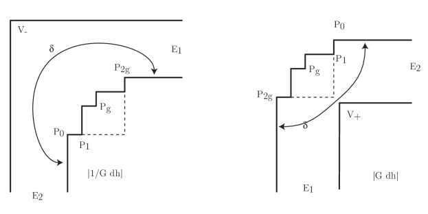
Figure 4.2. Orthodisk comparison

On the other hand, the corresponding orthodisk $\Omega_{G^{-1}dh}$ for $S_{g}$ sits strictly inside the corresponding orthodisk $\Omega_{G^{-1}dh}$ for $S_{1}$, using the standard correspondence of $\Omega_{Gdh}$ and $\Omega_{G^{-1}dh}$ orthodisks. Observe that for the $V_{i}$ close enough together, the vertex $V_{1}$ of $S_{1}$ will lie outside that of $\Omega_{G^{-1}dh}$ of $S_{g}$. Thus $\mathrm{ext}^{1}_{\Omega_{G^{-1}dh}}(\delta)\leq\mathrm{ext}^{1}_{\Omega_{G^{-1}dh}}(\delta)$.

Thus because we have $\mathrm{ext}_{\Omega_{G^{-1}dh}}^{1}(\delta)>\mathrm{ext}_{\Omega_{Gdh}}^{1}(\delta)$ for the case of $S_{1}$ (see (2.6)), with both quantities tending to zero (at different rates), the claim implies that we have the analogous inequality $\mathrm{ext}_{\Omega_{G^{-1}dh}}^{g}(\delta)>>\mathrm{ext}_{\Omega_{Gdh}}^{g}(\delta)$ holding for $S_{g}$. Moreover, the claim (and the notation) also implies that $\mathrm{ext}_{\Omega_{Gdh}}(\delta)$ tends to zero at a rate distinct from that of $\mathrm{ext}_{\Omega_{G^{-1}dh}}(\delta)$. Thus the height function $\operatorname{\mathcal{H}}(\delta)$ in such a case tends to infinity.

There is one final case to consider, which is hidden a bit because of our usual choice of conventions: it is only here that this normalizing of notation can be misleading. The issue is that, in Figure 4.2 for instance, the angle at $P_{g}$ and the angle of $V_{-}$ are both $\pi/2$ in $\Omega_{Gdh}$, and the angles are $3\pi/2$ at both $P_{g}$ and $V_{+}$ in $\Omega_{G^{-1}dh}$. However, we of course need to consider degenerations when the corresponding angles do not agree, for example when the angle at $P_{g}$ in $\Omega_{Gdh}$ is $3\pi/2$ while the angle at $V_{-}$ (also) in $\Omega_{Gdh}$ is $\pi/2$. [In that situation, we will also be in the situation where the angle at $P_{g}$ in $\Omega_{G^{-1}dh}$ is $\pi/2$ and the angle at $V_{+}$ in $\Omega_{G^{-1}dh}$ is $3\pi/2$.]

Now this situation is simply only a bit more complicated than the last case we considered, as it follows by applying the claim as before and then the comparison for genus one, only this time we have to apply that claim twice before invoking the comparison for genus one.

We also use a slightly different auxiliary construction, which we now explain. In the situation where the angle of $V_{-}$ in $\Omega_{Gdh}$ is $\pi/2$ while the angle at $P_{g}$ in $\Omega_{Gdh}$ is $3\pi/2$, imagine ‘cutting a notch out of $\Omega_{G^{-1}dh}$’ near $P_{g}$: more precisely, replace a neighborhood of $\partial\Omega_{Gdh}$ near $P_{g}$ with three vertices $P_{g-1}^{*},P_{g}^{*},P_{g+1}^{*}$ and edges between them that alternate $\pi/2$ and $3\pi/2$ angles in the usual way. This creates an orthodisk $\Omega_{Gdh}^{*}$ for a surface of quotient genus $g+1$, where the angle at $P_{g}^{*}$ is now $\pi/2$, now equaling the angle at $V_{-}$ opposite $P_{g}^{*}$. Of course, this notch-cutting also determines a conjugate domain $\Omega_{G^{-1}dh}^{*}$, where the angle at the (new) central point $P_{g}^{*}$ is now $3\pi/2$, also equaling the angle at $V_{+}$ opposite it. Thus, in considering the domains $\Omega_{Gdh}^{*}$ and $\Omega_{G^{-1}dh}^{*}$, we have returned to the third case we just finished considering. Fortunately, the comparisons between the extremal lengths on $\Omega_{Gdh}$ and $\Omega_{Gdh}^{*}$ and those between $\Omega_{G^{-1}dh}$ and $\Omega_{G^{-1}dh}^{*}$ allow for us to conclude that $\mathrm{ext}_{\Omega_{Gdh}}(\delta)>>\mathrm{ext}_{\Omega_{G^{-1}dh}}(\delta)$ as follows:

$$\mathrm{ext}_{\Omega_{Gdh}}(\delta) \geq\mathrm{ext}_{\Omega_{Gdh}}^{*}(\delta)\qquad$$ by the claimed principle

$$\geq\mathrm{ext}_{\Omega_{G^{-1}dh}}^{1}(\delta)$$ as in the third case

$$>>\mathrm{ext}_{\Omega_{Gdh}}^{1}(\delta)$$

$$\geq\mathrm{ext}_{\Omega_{G^{-1}dh}}^{*}(\delta)$$

$$\geq\mathrm{ext}_{\Omega_{G^{-1}dh}}(\delta)\qquad.$$

This treats the four possible cases, and the theorem is proven. ∎

4.3. A monodromy argument

In this section, we prove that the periods of orthodisks have incompatible logarithmic singularities in suitable coordinates and apply this to prove the Monodromy Theorem 4.6. The main idea is that to study the dependence of extremal lengths of the geometric coordinates, it is necessary to understand the asymptotic dependence of extremal lengths of the degenerating conformal polygons (which is classical and well-known, see [18]), and the asymptotic dependence of the geometric coordinates of the degenerating conformal polygons. This dependence is given by Schwarz-Christoffel maps which are well-studied in many special cases. Moreover, it is known that these maps possess asymptotic expansions in logarithmic terms. Instead of computing this expansion explicitly for the two maps we need, we use a monodromy argument to show that the crucial logarithmic terms have a different sign for the two expansions.

Let $\Delta_{g}$ be a geometric coordinate domain of dimension $g\geq 2$, i.e. a simply connected domain equipped with defining geometric coordinates for a pair of orthodisks $\Omega_{Gdh}$ and $\Omega_{G^{-1}dh}$ as usual.

Suppose $\gamma$ is a cycle in the underlying conformal polygon which joins two non-adjacent edges $P_{1}P_{2}$ with $Q_{1}Q_{2}$. Denote by $R_{1}$ the vertex before $Q_{1}$ and by $R_{2}$ the vertex after $Q_{2}$ and observe that by assumption, $R_{2}\neq P_{1}$ but that we can possibly have $P_{2}=R_{1}$. Introduce a second cycle $\beta$ which connects $R_{1}Q_{1}$ with $Q_{2}R_{2}$.

The situation is illustrated in the figure below; we have replaced the labels of $P_{i},V_{\pm}$ and $E_{j}$ that we use for vertices in $\partial\Omega_{Gdh}$ and $\partial\Omega_{G^{-1}dh}$ with generic labels of distinguished points on the boundary of the region: these will represent in general the situations that we would encounter in the orthodisk. Of course, we retain the convention of using the same label name for corresponding vertices in $\partial\Omega_{Gdh}$ and $\partial\Omega_{G^{-1}dh}$.

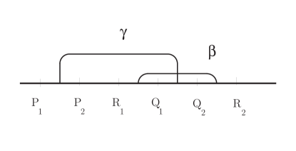
Figure 4.3. Monodromy argument

We formulate the claim of Theorem 4.6 more precisely in the following two lemmas:

Lemma 4.7.

Suppose that for a sequence $p_{n}\in\Delta$ with $p_{n}\to p_{0}\in\partial\Delta$ we have that $\mathrm{ext}_{\Omega_{Gdh}(p_{n})}(\gamma)\to 0$ and $\mathrm{ext}_{\Omega_{G^{-1}dh}(p_{n})}(\gamma)\to 0$. Suppose furthermore that $\gamma$ is a cycle encircling an edge which degenerates geometrically to $0$ as $n\to\infty$. Then

$$\left|e^{1/\mathrm{ext}_{\Omega_{Gdh}(p_{n})}(\gamma)}-e^{1/\mathrm{ext}_{\Omega_{G^{-1}dh}(p_{n})}(\gamma)}\right|^{2}\to\infty$$

Lemma 4.8.

Suppose that for a sequence $p_{n}\in\Delta$ with $p_{n}\to p_{0}\in\partial\Delta$ we have that $\mathrm{ext}_{\Omega_{Gdh}(p_{n})}(\gamma)\to\infty$ and $\mathrm{ext}_{\Omega_{G^{-1}dh}(p_{n})}(\gamma)\to\infty$. Suppose furthermore that $\gamma$ is a cycle footing on an edge which degenerates geometrically to $0$ as $n\to\infty$. Then

$$\left|e^{\mathrm{ext}_{\Omega_{Gdh}(p_{n})}(\gamma)}-e^{\mathrm{ext}_{\Omega_{G^{-1}dh}(p_{n})}(\gamma)}\right|^{2}\to\infty$$

Proof.

We first prove Lemma 4.7.

Consider the conformal polygons corresponding to the pair of orthodisks. Normalize the punctures by Möbius transformations so that

$$P_{1}=-\infty,P_{2}=0,Q_{1}=\epsilon,Q_{2}=1$$

for $\Omega_{Gdh}$ and

$$P_{1}=-\infty,P_{2}=0,Q_{1}=\epsilon^{\prime},Q_{2}=1$$

for $\Omega_{G^{-1}dh}$.

If $\alpha$ is a curve in a domain $\Omega\subset\mathbb{C}$, then define $\operatorname{Per}\alpha(\Omega)=\int_{\alpha}dz$. Here our focus is on periods of the one-form $dz$ as we are typically interested in domains $\Omega$ which are developed images of pairs $(\Omega,\omega)$ of domains and one-forms on those domains, i.e. $z(p)=\int_{p_{0}}^{p}\omega$. By the assumption of Lemma 4.7, we know that $\epsilon,\epsilon^{\prime}\to 0$ as $n\to\infty$.

We now allow $Q_{1}$ to move in the complex plane and apply the Real Analyticity Alternative Lemma 4.11 below to the curve $\epsilon=\epsilon_{0}e^{it}$: here we are regarding the position of $Q_{1}$ as traveling along a small circle around the origin, i.e. its defined position $\epsilon\in\mathbb{R}$ has been extended to allow complex values. We will conclude from that lemma that either

(4.1) $$\frac{|\operatorname{Per}\gamma(\Omega_{Gdh})|}{|\operatorname{Per}\beta(\Omega_{Gdh})|}+\frac{1}{\pi}\log\epsilon=:F_{1}(\epsilon)$$

is single-valued in $\epsilon$ and

(4.2) $$\frac{|\operatorname{Per}\gamma(\Omega_{G^{-1}dh})|}{|\operatorname{Per}\beta(\Omega_{G^{-1}dh})|}-\frac{1}{\pi}\log\epsilon^{\prime}=:F_{2}(\epsilon^{\prime})=F_{2}(\epsilon^{\prime}(\epsilon))$$

is single-valued in $\epsilon^{\prime}$ or vice versa, with signs exchanged. Without loss of generality, we can treat the first case.

Now suppose that $\epsilon^{\prime}$ is real analytic (and hence single-valued) in $\epsilon$ and comparable to $\epsilon$ near $\epsilon=0$. Then using that $\Omega_{Gdh}$ and $\Omega_{G^{-1}dh}$ are conjugate implies that

$$\frac{|\operatorname{Per}\gamma(\Omega_{Gdh})|}{|\operatorname{Per}\beta(\Omega_{Gdh})|}=\frac{|\operatorname{Per}\gamma(\Omega_{G^{-1}dh})|}{|\operatorname{Per}\beta(\Omega_{G^{-1}dh})|}\ .$$

By subtracting the function $F_{1}(\epsilon)$ in 4.1 from the function $F_{2}(\epsilon^{\prime})$ in 4.2 (both of which are single-valued in $\epsilon$) we get that

$$\log(\epsilon\epsilon^{\prime}(\epsilon))$$

is single-valued in $\epsilon$ near $\epsilon=0$ which contradicts that $\epsilon,\epsilon^{\prime}\to 0$.

Now Ohtsuka’s extremal length formula states that for the current normalization of $\Omega_{Gdh}(p_{n})$ we have

$$\mathrm{ext}(\gamma)=O\left(\log|\epsilon|\right)$$

(see [18]). We conclude that

$$|e^{1/\mathrm{ext}_{\Omega_{Gdh}(p_{n})}(\gamma)}-e^{1/\mathrm{ext}_{\Omega_{G^{-1}dh}(p_{n})}(\gamma)}|=O\left(\frac{1}{\epsilon}-\frac{1}{\epsilon^{\prime}}\right)$$

which goes to infinity, since we have shown that $\epsilon$ and $\epsilon^{\prime}$ tend to zero at different rates. This proves Lemma 4.7.

The proof of Lemma 4.8 is very similar: For convenience, we normalize the points of the punctured disks such that

$$P_{1}=-\infty,P_{2}=0,Q_{1}=1,Q_{2}=1+\epsilon$$

for $\Omega_{Gdh}$ and

$$P_{1}=-\infty,P_{2}=0,Q_{1}=1,Q_{2}=1+\epsilon^{\prime}$$

for $\Omega_{G^{-1}dh}$.

By the assumption of Lemma 4.8, we know that $\epsilon,\epsilon^{\prime}\to 0$ as $n\to\infty$. We now apply the Real Analyticity Alternative Lemma 4.11 below to the curve $1+\epsilon_{0}e^{it}$ and conclude that

$$\frac{\operatorname{Per}\gamma(\Omega_{Gdh})}{\operatorname{Per}\beta(\Omega_{Gdh})}+\frac{1}{\pi}\log\epsilon$$

is single-valued in $\epsilon$ while

$$\frac{\operatorname{Per}\gamma(\Omega_{G^{-1}dh})}{\operatorname{Per}\beta(\Omega_{G^{-1}dh})}-\frac{1}{\pi}\log\epsilon^{\prime}$$

is single-valued in $\epsilon^{\prime}$. The rest of the proof is identical to the proof of Lemma 4.7. ∎

To prove the needed Real Analyticity Alternative Lemma 4.11, we need asymptotic expansions of the extremal length in terms of the geometric coordinates of the orthodisks. Though not much is known explicitly about extremal lengths in general, for the chosen cycles we can reduce this problem to an asymptotic control of Schwarz-Christoffel integrals. Their monodromy properties allow us to distinguish their asymptotic behavior by the sign of logarithmic terms.

We introduce some notation: suppose we have an orthodisk such that the angles at the vertices alternate between $\pi/2$ and $-\pi/2$ modulo $2\pi$. (We will also allow some angles to be $0$ modulo $2\pi$ but they will not be relevant for this argument.) Consider the Schwarz-Christoffel map

$$F:z\mapsto\int^{z}(t-t_{1})^{a_{1}/2}\cdot\ldots\cdot(t-t_{n})^{a_{n}/2}\,dt$$

from a conformal polygon with vertices at $t_{i}$ to this orthodisk: here the exponents $a_{j}$ alternate between $-1$ and $+1$, depending on whether the angles at the vertices are $\pi/2$ or $-\pi/2,\pmod{2\pi}$, respectively. Choose four distinct vertices $t_{i},t_{i+1},t_{j},t_{j+1}$ (not necessarily consecutive). Introduce a cycle $\gamma$ in the upper half plane connecting edge $(t_{i},t_{i+1})$ with edge $(t_{j},t_{j+1})$ and denote by $\bar{\gamma}$ the closed cycle obtained from $\gamma$ and its mirror image at the real axis. Similarly, denote by $\beta$ the cycle connecting $(t_{j-1},t_{j})$ with $(t_{j+1},t_{j+2})$ and by $\bar{\beta}$ the cycle together with its mirror image.

Now consider the Schwarz-Christoffel period integrals

$$F(\gamma) =\frac{1}{2}\int_{\bar{\gamma}}(t-t_{1})^{a_{1}/2}\cdot\ldots\cdot(t-t_{n})^{a_{n}/2}dt$$

$$F(\beta) =\frac{1}{2}\int_{\bar{\beta}}(t-t_{1})^{a_{1}/2}\cdot\ldots\cdot(t-t_{n})^{a_{n}/2}dt$$

as multivalued functions depending on the now complex parameters $t_{i}$.

Lemma 4.9.

Under analytic continuation of $t_{j+1}$ around $t_{j}$ the periods change their values like

$$F(\gamma) \rightarrow F(\gamma)+2F(\beta)$$

$$F(\beta) \rightarrow F(\beta)$$

Proof.

The path of analytic continuation of $t_{j+1}$ around $t_{j}$ gives rise to an isotopy of $\mathbb{C}$ which moves $t_{j+1}$ along this path. This isotopy drags $\beta$ and $\gamma$ to new cycles $\beta^{\prime}$ and $\gamma^{\prime}$.

Because the curve $\beta$ is defined to surround $t_{j}$ and $t_{j+1}$, the analytic continuation merely returns $\beta$ to $\beta^{\prime}$. Thus, because $\beta^{\prime}$ equals $\beta$, their periods are also equal. On the other hand, the curve $\gamma$ is not equal to $\gamma^{\prime}$: informally, $\gamma^{\prime}$ is obtained as the Dehn twist of $\gamma$ around $\bar{\beta}$. Now, the period of $\gamma^{\prime}$ is obtained by developing the flat structure of the doubled orthodisk along $\gamma^{\prime}$. To compute this flat structure, observe the crucial fact that the angles at the orthodisk vertices are either $\pi/2$ or $-\pi/2$, modulo $2\pi$. In either case, we see from the developed flat structure that the period of $\gamma^{\prime}$ equals the period of $\gamma$ plus twice the period of $\beta$. ∎

Now denote by $\delta:=t_{j+1}-t_{j}$ and fix all $t_{i}$ other than $t_{j+1}$: we regard $t_{j+1}$ as the independent variable, here viewed as complex, since we are allowing it to travel around $t_{j}$.

Lemma 4.10 (Analyticity Lemma).

The function $F(\gamma)-\frac{\log\delta}{\pi i}F(\beta)$ is single-valued and holomorphic in $\delta$ in a neighborhood of $\delta=0$.

Proof.

By definition,the function is locally holomorphic in a punctured neighborhood of $\delta=0$. By Lemma 4.9 it extends to be single valued in a (full) neighborhood of $\delta=0$. ∎

We will now specialize this picture to the situation at hand — an orthodisk where $\gamma$ represents one of the distinguished cycles $\gamma_{i}$. Then $F(\gamma)$ and $F(\beta)$ are either real or imaginary, and are perpendicular. Thus Lemma 4.10 implies that $|F(\gamma)|\pm\frac{\log\delta}{\pi}|F(\beta)|$ is real analytic in $\delta$ with one choice of sign. The crucial observation is now that whatever alternative holds, the opposite alternative will hold for the conjugate orthodisk. More precisely:

Let $F_{1}$ and $F_{2}$ be the Schwarz-Christoffel maps associated to a pair of conjugate orthodisks. These will be defined on different but consistently labeled punctured upper half planes. Let $\delta_{i}$ refer to the complex parameter $\delta$ introduced above for the maps $F_{i}$, respectively. Then

Lemma 4.11 (Real Analyticity Alternative Lemma).

Either $|F_{1}(\gamma)|-\frac{\log\delta_{1}}{\pi}|F_{1}(\beta)|$ or $|F_{1}(\gamma)|+\frac{\log\delta_{1}}{\pi}|F_{1}(\beta)|$ is real analytic in $\delta_{1}$ for $\delta_{1}=0$. In the first case, $|F_{2}(\gamma)|+\frac{\log\delta_{2}}{\pi}|F_{2}(\beta)|$ is real analytic in $\delta_{2}$, while in the second case, $|F_{2}(\gamma)|-\frac{\log\delta}{\pi}|F_{2}(\beta)|$ is real-analytic in $\delta_{2}$.

Proof.

We have already noted that either alternative holds in both cases. It remains to show that it holds with opposite signs. For some special values $\delta_{1},\delta_{2}>0$, the two orthodisks are conjugate. For instance, we can assume that for these values, $F_{1}(\gamma)=F_{2}(\gamma)>0$. Then $F_{1}(\beta)$ and $F_{2}(\beta)$ are both imaginary with opposite signs, and the claimed alternative holds for these values of $\delta_{1},\delta_{2}$. By continuity, the alternative holds for all $\delta_{1}$ and $\delta_{2}$. ∎

Remark 4.12.

A concrete way of understanding the phenomenon here is that the asymptotic expansion of the period of a curve meeting a degenerating cycle $\beta$, where the edge for $\beta$ has preimages $b$ and $b+\epsilon$, has a term of the form $\pm\epsilon^{k}\log\epsilon$, where the sign relates to the geometry of the orthodisk.

5. The Flow to a Solution

The last part of the proof of the Main Theorem requires us to prove the

Lemma 5.1 (Regeneration Lemma).

There is, for a given genus $g$, a certain (good) locus $\mathcal{Y}\subset\Delta_{g}$ in the space $\Delta_{g}$ of geometric coordinates for with the following properties:

• $\mathcal{Y}$ lies properly within the space of geometric coordinates;

• if $d\operatorname{\mathcal{H}}=0$ at a point on the locus $\mathcal{Y}$, then actually $\operatorname{\mathcal{H}}=0$ at that point.

This locus will be defined by the requirement that all but one of the extremal lengths of the distinguished cycles of the $Gdh$ and $\frac{1}{G}dh$ orthodisks are equal.

5.1. Overall Strategy

In this section we continue the proof of the existence of the surfaces $\{S_{g}\}$. In the previous sections, we defined an associated moduli space $\Delta=\Delta_{g}$ of pairs of conformal structures $\{\Omega_{Gdh},\Omega_{G^{-1}dh}\}$ equipped with geometric coordinates $\vec{\mathbb{t}}=(t_{i},...,t_{g})$.

We defined a height function $\operatorname{\mathcal{H}}$ on the moduli space $\Delta$ and proved that it was a proper function: as a result, there is a critical point for the height function in $\Delta$, and our overall goal in the next pair of sections is a proof that this critical point represents a reflexive orthodisk system in $\Delta$, and hence, by our fundamental translation of the period problem for minimal surfaces into a conformal equivalence problem, a minimal surface of the form $S_{g}$. Our goal in the present section is a description of the tangent space to the the moduli space $\Delta$: we wish to display how infinitesimal changes in the geometric coordinates $\vec{\mathbb{t}}$ affect the height function. In particular, it would certainly be sufficient for our purposes to prove the statement

Model 5.2.

If $\vec{\mathbb{t}_{0}}$ is not a reflexive orthodisk system, then there is an element $V$ of the tangent space $T_{\vec{\mathbb{t}_{0}}}\Delta$ for which $D_{V}\operatorname{\mathcal{H}}\neq 0$.

This would then have the effect of proving that our critical point for the height function is reflexive, concluding the existence parts of the proofs of the main theorem.

We do not know how to prove or disprove this model statement in its full generality. On the other hand, it is not necessary for the proofs of the main theorems that we do so. Instead we will replace this statement by a pair of lemmas.

Lemma 5.3.

Let $\mathcal{Y}\subset\Delta$ is a real one-dimensional subspace of $\Delta$ which is defined by the equations $\operatorname{\mathcal{H}}(\gamma_{1})=\operatorname{\mathcal{H}}(\gamma_{2})=...=\operatorname{\mathcal{H}}(\gamma_{g-2})=\operatorname{\mathcal{H}}(\delta)=0$. If $\vec{\mathbb{t}_{0}}\in\mathcal{Y}$ has positive height, i.e. $\operatorname{\mathcal{H}}(\vec{\mathbb{t}_{0}})>0$, then there is an element $V$ of the tangent space $T_{\vec{\mathbb{t}_{0}}}\mathcal{Y}$ for which $D_{V}\operatorname{\mathcal{H}}\neq 0$.

Lemma 5.4.

There is an analytic subspace $\mathcal{Y}\subset\Delta=\Delta_{g}$, for which $\mathcal{Y}=\{\operatorname{\mathcal{H}}(\gamma_{1})=\operatorname{\mathcal{H}}(\gamma_{2})=...=\operatorname{\mathcal{H}}(\gamma_{g-2})=\operatorname{\mathcal{H}}(\delta)=0\}$.

Given these lemmas, the proof of the existence of a pair of conformal orthodisks $\{\Omega_{Gdh},\Omega_{G^{-1}dh}\}$ is straightforward.

Proof.

Proof of Existence of Reflexive Orthodisks. Consider the locus $\mathcal{Y}$ guaranteed by Lemma 5.4. By Theorem 4.5, the height function $\operatorname{\mathcal{H}}$ is proper on $\mathcal{Y}$, so the height function $\operatorname{\mathcal{H}}|_{\mathcal{Y}}$ has a critical point (on $\mathcal{Y}$). By Lemma 5.3, this critical point represents a point of $\operatorname{\mathcal{H}}=0$, i.e a reflexive orthodisk by Lemma 4.3. ∎

The proof of Lemma 5.3 occupies the current section while the proof of Lemma 5.4 is given in the following section.

Remarks on deformations of conjugate pairs of orthodisks. Let us discuss informally the proof of Lemma 5.3. Because angles of corresponding vertices in the $\Omega_{Gdh}\leftrightarrow\Omega_{G^{-1}dh}$ correspondence sum to $0\pmod{2\pi}$, the orthodisks fit together along corresponding edges, so conjugacy of orthodisks requires corresponding edges to move in different directions: if the edge $E$ on $\Omega_{Gdh}$ moves “out,” the corresponding edge $E^{*}$ on $\Omega_{G^{-1}dh}$ edge moves “in”, and vice versa (see the figures below). Thus we expect that if $\gamma$ has an endpoint on $E$, then one of the extremal lengths of $\gamma$ decreases, while the other extremal length of $\gamma$ on the other orthodisk would increase: this will force the height $\operatorname{\mathcal{H}}(\gamma)$ of $\gamma$ to have a definite sign, as desired. This is the intuition behind Lemma 5.3; a rigorous argument requires us to actually compute derivatives of relevant extremal lengths using the formula 2.3. We do this by displaying, fairly explicitly, the deformations of the orthodisks (in local coordinates on $\Omega_{Gdh}/\Omega_{G^{-1}dh}$) as well as the differentials of extremal lengths, also in coordinates. After some preliminary notational description in section 5.2, we do most of the computing in section 5.3. Also in section 5.3 is the key technical lemma, which relates the formalism of formula 2.3, together with the local coordinate descriptions of its terms, to the intuition we just described.

5.2. Infinitesimal pushes

We need to formalize the previous discussion. As always we are concerned with relating the Euclidean geometry of the orthodisks (which corresponds directly with the periods of the Weierstrass data) to the conformal data of the domains $\Omega_{Gdh}$ and $\Omega_{G^{-1}dh}$. From the discussion above, it is clear that the allowable infinitesimal motions in $\Delta$, which are parametrized in terms of the Euclidean geometry of $\Omega_{Gdh}$ and $\Omega_{G^{-1}dh}$, are given by infinitesimal changes in lengths of finite sides, with the changes being done simultaneously on $\Omega_{Gdh}$ and $\Omega_{G^{-1}dh}$ to preserve conjugacy. The link to the conformal geometry is the formula 2.3: a motion which infinitesimally transforms $\Omega_{Gdh}$, say, will produce an infinitesimal change in the conformal structure. This tangent vector to the moduli space of conformal structures is represented by a Beltrami differential. Later, formula 2.3 will be used, together with knowledge of the cotangent vectors $d\mathrm{ext}_{\Omega_{Gdh}}(\cdot)$ and $d\mathrm{ext}_{\Omega_{G^{-1}dh}}(\cdot)$, to determine the derivatives of the relevant extremal lengths, hence the derivative of the height.

To begin, we explicitly compute the effect of infinitesimal pushes of certain edges on the extremal lengths of relevant cycles. This is done by explicitly displaying the infinitesimal deformation and then using this formula to compute the sign of the derivative of the extremal lengths, using formula 2.3. There will be two different cases to consider.

1. Finite non-central edges of the type $P_{i-1}P_{i}$ for $i<g$.

2. An edge (finite or infinite) and its symmetric side meet in a corner, for instance $P_{g-1}P_{g}$.

For each case there are two subcases, which we can describe as depending on whether the given sides are horizontal or vertical. The distinction is, surprisingly, a bit important, as together with the fact that we do our deformations in pairs, it provides for an important cancelation of (possibly) singular terms in Lemma 5.5. We defer this point for later, while here we begin to calculate the relevant Beltrami differentials in the cases.

While logically it is conceivable that each infinitesimal motion might require two different types of cases, depending on whether the edge we are deforming on $\Omega_{Gdh}$ corresponds on $\Omega_{G^{-1}dh}$ to an edge of the same type or a different type, in fact this issue does not arise for the particular case of the Scherk surfaces we are discussing in this paper. By contrast, it does arise for the generalized Costa surfaces we discussed in [29].

Case A. Here the computations are quite analogous to those that we found in [28]; they differ only in orientation of the boundary of the orthodisk. We include them for the completeness of the exposition.

Figure 5.1. Beltrami differential computation — case A

We first consider the case of a horizontal finite side; as in the figure above, we see that the neighborhood of the horizontal side of the orthodisk in the plane naturally divides into six regions which we label $R_{1}$,…,$R_{6}$. Our deformation $f_{\epsilon}=f_{\epsilon,b,\delta}$ differs from the identity only in such a neighborhood, and in each of the six regions, the map is affine. In fact we have a two-parameter family of these deformations, all of which have the same infinitesimal effect, with the parameters $b$ and $\delta$ depending on the dimensions of the supporting neighborhood.

(5.1) $$f_{\epsilon}(x,y)=\begin{cases}\left(x,\epsilon+\frac{b-\epsilon}{b}y\right),&\{-a\leq x\leq a,0\leq y\leq b\}=R_{1}\\ \left(x,\epsilon+\frac{b+\epsilon}{b}y\right),&\{-a\leq x\leq a,-b\leq y\leq 0\}=R_{2}\\ \left(x,y+\frac{\epsilon+\frac{b-\epsilon}{b}y-y}{\delta}(x+\delta+a)\right),&\{-a-\delta\leq x\leq-a,0\leq y\leq b\}=R_{3}\\ \left(x,y-\frac{\epsilon+\frac{b-\epsilon}{b}y-y}{\delta}(x-\delta-a)\right),&\{a\leq x\leq a+\delta,0\leq y\leq b\}=R_{4}\\ \left(x,y+\frac{\epsilon+\frac{b+\epsilon}{b}y-y}{\delta}(x+\delta+a)\right),&\{-a-\delta\leq x\leq-a,-b\leq y\leq 0\}=R_{5}\\ \left(x,y-\frac{\epsilon+\frac{b+\epsilon}{b}y-y}{\delta}(x-\delta-a)\right),&\{a\leq x\leq a+\delta,-b\leq y\leq 0\}=R_{6}\\ (x,y)&\text{otherwise}\end{cases}$$

where we have defined the regions $R_{1},\dots,R_{6}$ within the definition of $f_{\epsilon}$. Also note that here the orthodisk contains the arc $\{(-a,y)\mid 0\leq y\leq b\}\cup\{(x,0)\mid-a\leq x\leq a\}\cup\{(a,y)\mid-b\leq y\leq 0\}$. Let $E$ denote the edge being pushed, defined above as $[-a,a]\times\{0\}$.

Of course $f_{\epsilon}$ differs from the identity only on a neighborhood of the edge $E$, so that $f_{\epsilon}$ takes the symmetric orthodisk to an asymmetric orthodisk. We next modify $f_{\epsilon}$ in a neighborhood of the reflected (across the $y=-x$ line) segment $E^{*}$ in an analogous way with a map $f^{*}_{\epsilon}$ so that $f^{*}_{\epsilon}\circ f_{\epsilon}$ will preserve the symmetry of the orthodisk.

Our present conventions are that the edge $E$ is horizontal; this forces $E^{*}$ to be vertical and we now write down $f^{*}_{\epsilon}$ for such a vertical segment; this is a straightforward extension of the description of $f_{\epsilon}$ for a horizontal side, but we present the definition of $f^{*}_{\epsilon}$ anyway, as we are crucially interested in the signs of the terms. So set

(5.2) $$f^{*}_{\epsilon}=\begin{cases}\left(-\epsilon+\frac{b-\epsilon}{b}x,y\right),&\{-b\leq x\leq 0,-a\leq y\leq a\}=R^{*}_{1}\\ \left(-\epsilon+\frac{b+\epsilon}{b}x,y\right),&\{0\leq x\leq b,-a\leq y\leq a\}=R^{*}_{2}\\ \left(x-\frac{-\epsilon+\frac{b-\epsilon}{b}x-x}{\delta}(y-\delta-a),y\right),&\{-b\leq x\leq 0,a\leq y\leq a+\delta\}=R^{*}_{3}\\ \left(x+\frac{-\epsilon+\frac{b-\epsilon}{b}x-x}{\delta}(y+\delta+a),y\right),&\{-b\leq x\leq 0,-a-\delta\leq y\leq-a\}=R^{*}_{4}\\ \left(x-\frac{-\epsilon+\frac{b+\epsilon}{b}x-x}{\delta}(y-\delta-a),y\right),&\{0\leq x\leq b,a\leq y\leq a+\delta\}=R^{*}_{5}\\ \left(x+\frac{-\epsilon+\frac{b+\epsilon}{b}x-x}{\delta}(y+\delta+a),y\right),&\{0\leq x\leq b,-a-\delta\leq y\leq-a\}=R^{*}_{6}\\ (x,y)&\text{otherwise}\end{cases}$$

Note that under the reflection across the line $\{y=-x\}$, the region $R_{i}$ gets taken to the region $R_{i}^{*}$.

Let $\nu_{\epsilon}=\frac{\left(f_{\epsilon}\right)_{\bar{z}}}{\left(f_{\epsilon}\right)_{z}}$ denote the Beltrami differential of $f_{\epsilon}$, and set $\dot{\nu}=\frac{d}{d\epsilon}\bigm{|}_{\epsilon=0}\nu_{\epsilon}$. Similarly, let $\nu^{*}_{\epsilon}$ denote the Beltrami differential of $f^{*}_{\epsilon}$, and set $\dot{\nu}^{*}=\frac{d}{d\epsilon}\bigm{|}_{\epsilon=0}\nu^{*}_{\epsilon}$. Let $\dot{\mu}=\dot{\nu}+\dot{\nu}^{*}$. Now $\dot{\mu}$ is a Beltrami differential supported in a bounded domain in one of the domains $\Omega_{Gdh}$ or $\Omega_{G^{-1}dh}$. We begin by observing that it is easy to compute that $\dot{\nu}=[\frac{d}{d\epsilon}\bigm{|}_{\epsilon=0}\left(f_{\epsilon}\right)]_{\bar{z}}$ evaluates near $E$ to

(5.3) $$\dot{\nu}=\begin{cases}\frac{1}{2b},&z\in R_{1}\\ -\frac{1}{2b},&z\in R_{2}\\ \frac{1}{2b}[x+\delta+a]/\delta+i\left(1-y/b\right)\frac{1}{2\delta}=\frac{1}{2b\delta}(\bar{z}+\delta+a+ib),&z\in R_{3}\\ -\frac{1}{2b}[x-\delta-a]/\delta-i\left(1-y/b\right)\frac{1}{2\delta}=\frac{1}{2b\delta}(-\bar{z}+\delta+a-ib),&z\in R_{4}\\ -\frac{1}{2b}[x+\delta d+a]/\delta+i\left(1+y/b\right)\frac{1}{2\delta}=\frac{1}{2b\delta}(-\bar{z}-\delta-a+ib),&z\in R_{5}\\ \frac{1}{2b}[x-\delta-a]/\delta-i\left(1+y/b\right)\frac{1}{2\delta}=\frac{1}{2b\delta}(\bar{z}-\delta-a-ib),&z\in R_{6}\\ 0&z\notin\operatorname{supp}(f_{\epsilon}-\operatorname{id})\end{cases}$$

We further compute

(5.4) $$\dot{\nu}^{*}=\begin{cases}-\frac{1}{2b},&R^{*}_{1}\\ \frac{1}{2b},&R^{*}_{2}\\ \frac{1}{2b\delta}(i\bar{z}-\delta-a+bi)&R^{*}_{3}\\ \frac{1}{2b\delta}(-i\bar{z}-\delta-a-bi)&R^{*}_{4}\\ \frac{1}{2b\delta}(-i\bar{z}+\delta+a+bi)&R^{*}_{5}\\ \frac{1}{2b\delta}(i\bar{z}+\delta+a-bi)&R^{*}_{6}\end{cases}$$

Case B. We have separated this case out for purely expositional reasons. We can imagine that the infinitesimal push that moves the pair of consecutive sides along the symmetry line $\{y=-x\}$ is the result of a composition of a pair of pushes from Case A, i.e. our diffeomorphism $F_{\epsilon;b,\delta}$ can be written $F_{\epsilon;b,\delta}=f_{\epsilon}\circ f_{\epsilon}^{*}$, where the maps differ from the identity in the union of the supports of $\dot{\nu}_{b,\delta}$ and $\dot{\nu}_{b,\delta}^{*}$.

It is an easy consequence of the chain rule applied to this formula for $F_{\epsilon;b,\delta}$ that the infinitesimal Beltrami differential for this deformation is the sum $\dot{\nu}_{b,\delta}+\dot{\nu}_{b,\delta}^{*}$ of the infinitesimal Beltrami differentials $\dot{\nu}_{b,\delta}$ and $\dot{\nu}_{b,\delta}^{*}$ defined in formulae 5.3, 5.4 for Case A (even in a neighborhood of the vertex along the diagonal where the supports of the differentials $\dot{\nu}_{b,\delta}$ and $\dot{\nu}_{b,\delta}^{*}$ coincide).

5.3. Derivatives of Extremal Lengths

In this section, we combine the computations of $\dot{\nu}_{b,\delta}$ with formula 2.3 (and its background in section 2) and some easy observations on the nature of the quadratic differentials $\Phi_{\mu}=\frac{1}{2}d\mathrm{ext}_{(\cdot)}(\mu)\bigm{|}_{\cdot}$ to compute the derivatives of extremal lengths under our infinitesimal deformations of edge lengths.

We begin by recalling some background from section 2. If we are given a curve $\gamma$, the extremal length of that curve on an orthodisk, say $\Omega_{Gdh}$, is a real-valued $C^{1}$ function on the moduli space of that orthodisk. Its differential is then a holomorphic quadratic differential $\Phi_{\gamma}=\frac{1}{2}d\mathrm{ext}_{(\cdot)}(\gamma)\bigm{|}_{\Omega_{Gdh}}$ on that orthodisk; the horizontal foliation of $\Phi_{\gamma}$ consists of curves which connect the same edges in $\Omega_{Gdh}$ as $\gamma$, since $\Phi_{\gamma}$ is obtained as the pullback of the quadratic differential $dz^{2}$ from a rectangle where $\gamma$ connects the opposite vertical sides. We compute the derivative of the extremal length function using formula 2.3, i.e.

$$\left(d\mathrm{ext}_{\cdot}(\gamma)\bigm{|}_{\Omega_{Gdh}}\right)[\nu]=4\operatorname{Re}\int_{\Omega_{Gdh}}\Phi_{\gamma}\nu$$

It is here where we find that we can actually compute the sign of the derivative of the extremal lengths, hence the height function, but also encounter a subtle technical problem. The point is that we will discover that just the topology of the curve $\gamma$ on $\Omega_{Gdh}$ will determine the sign of the derivative on an edge $E$, so we will be able to evaluate the sign of the integral above, if we shrink the support of the Beltrami differential $\dot{\nu}_{b,\delta}$ to the edge by sending $b,\delta$ to zero. (In particular, the sign of $\Phi_{\gamma}$ depends precisely on whether the foliation of $\Phi=\Phi_{\gamma}$ is parallel or perpendicular to $E$, and on whether $E$ is horizontal or vertical.) We then need to know two things: 1) that this limit exists, and 2) that we may know its sign via examination of the sign of $\dot{\nu}_{b,\delta}$ and $\Phi_{\gamma}$ on the edge $E$. We phrase this as

Lemma 5.5.

(1) $\lim_{b\to 0,\delta\to 0}\operatorname{Re}\int\Phi\dot{\nu}$ exists, is finite and non-zero. (2) The (horizontal) foliation of $\Phi=\Phi_{\gamma}$ is either parallel or orthogonal to the segment which is $\lim_{b\to 0,\delta\to 0}(\operatorname{supp}\dot{\nu})$, and (3) The expression $\Psi\dot{\nu}$ has a constant sign on the that segment $E$, and the integral 2.3 also has that (same) sign.

Of course, in the statement of the lemma, the horizontal foliation of the holomorphic quadratic differential $\Phi=\Phi_{\gamma}$ has regular curves parallel to $\gamma$.

This lemma provides the rigorous foundation for the intuition described in the final paragraph of strategy section 5.1.

5.4. Proof of the Technical Lemma 5.5

Proof.

Let $S_{Gdh}$ denote the double of $\Omega_{Gdh}$ across the boundary; the metric space $S_{Gdh}$ is a flat sphere with conical singularities, two of which are metric cylinders.

The foliation of $\Phi$, on say $\Omega_{Gdh}$, lifts to a foliation on the punctured sphere, symmetric about the reflection about the equator. This proves the second statement. The third statement follows from the first (and from the above discussion of the topology of the vertical foliation of $\Phi_{\gamma}$), once we prove that there is no infinitude of $\int\Phi\dot{\nu}$ as $b,\delta\to 0$ coming from either the neighborhood of infinity of the infinite edges or the regions $R_{3}$ and $R_{4}$ for the finite vertices. This finiteness will follow from the proof of the first statement. Thus, we are left to prove the first statement which requires us once again to consider the cases A and B.

Case A: Suppose $\gamma$ connects two non-central finite edges $E^{\prime}$ and $E^{\prime\prime}$ on $\Omega_{Gdh}$. To understand the singular behavior of $\Phi=\Phi_{\gamma}$ near a vertex of the orthodisk, say $\Omega_{Gdh}$, we begin by observing (by formula 2.3) that on a preimage on $S_{Gdh}$ of such a vertex, the lifted quadratic differential, say $\Psi$, has a simple pole. This is consistent with the nature of the foliation of $\Psi$, whose non-singular horizontal leaves are all freely homotopic to the lift of $\gamma$; the fact itself follows from following the lift of the canonical quadratic differential on a rectangle. Thus the singular leaves of $\Psi$ are segments on the equator of the sphere connecting lifts of endpoints of the edges $E^{\prime}$ and $E^{\prime\prime}$.

Now let $\omega$ be a local uniformizing parameter near the preimage of the vertex on $S_{Gdh}$ and $\zeta$ a local uniformizing parameter near the vertex of $\Omega_{Gdh}$ on $\mathbb{C}$. There are two cases to consider, depending on whether the angle in $\Omega_{Gdh}$ at the vertex is $3\pi/2$ or $\pi/2$. In the first case, the map from $\Omega_{Gdh}$ to a lift of $\Omega_{Gdh}$ in $S_{Gdh}$ is given in coordinates by $\omega=(i\zeta)^{2/3}$, and in the second case by $\omega=\zeta^{2}$. Thus, in the first case we write $\Psi=c\frac{d\omega^{2}}{\omega}$ so that $\Phi=-4/9c(i\zeta)^{-4/3}d\zeta^{2}$, and in the second case we write $\Phi=4cd\zeta^{2}$; in both cases, the constant $c$ is real with sign determined by the direction of the foliation.

With these expansions for $\Phi$, we can compute $\lim_{b\to 0,\delta\to 0}\operatorname{Re}\int\Phi\dot{\nu}$.

Clearly, as $b+\delta\to 0$, as $|\dot{\nu}|=O\left(\max\left(\frac{1}{b},\frac{1}{\delta}\right)\right)$, we need only concern ourselves with the contribution to the integrals of the singularity at the vertices of $\Omega_{Gdh}$ with angle $3\pi/2$.

To begin this analysis, recall that we have assumed that the edge $E$ is horizontal so that $\Omega_{Gdh}$ has a vertex angle of $3\pi/2$ at the vertex, say $P$. This means that $\Omega_{Gdh}$ also has a vertex angle of $3\pi/2$ at the reflected vertex, say $P^{*}$, on $E^{*}$. It is convenient to rotate a neighborhood of $E^{*}$ through an angle of $-\pi/2$ so that the support of $\dot{\nu}$ is a reflection of the support of $\dot{\nu}^{*}$ (see equation 5.1 through a vertical line. If the coordinates of $\operatorname{supp}\dot{\nu}$ and $\operatorname{supp}\dot{\nu}^{*}$ are $z$ and $z^{*}$, respectively (with $z(P)=z^{*}(P^{*})=0$), then the maps which lift neighborhoods of $P$ and $P^{*}$, respectively, to the sphere $S_{Gdh}$ are given by

$$z\mapsto(iz)^{2/3}=\omega\quad\hbox{ and}\quad z^{*}\mapsto(z^{*})^{2/3}=\omega^{*}.$$

Now the poles on $S_{Gdh}$ have coefficients $c\frac{d\omega^{2}}{\omega}$ and $-c\frac{d\omega^{*2}}{\omega^{*}}$, respectively, so we find that when we pull back these poles from $S_{Gdh}$ to $\Omega_{Gdh}$, we have $\Phi(z)=-\frac{4}{9}c\ {dz^{2}}/{\omega^{2}}$ while $\Phi(z^{*})=-\frac{4}{9}c\ dz^{2}/(\omega^{*})^{2}$ in the coordinates $z$ and $z^{*}$ for $\operatorname{supp}\dot{\nu}$ and $\operatorname{supp}\dot{\nu}^{*}$, respectively. But by tracing through the conformal maps $z\mapsto\omega\mapsto\omega^{2}$ on $\operatorname{supp}\dot{\nu}$ and $z^{*}\mapsto\omega^{*}\mapsto(\omega^{*})^{2}$, we see that if $z^{*}$ is the reflection of $z$ through a line, then

$$\frac{1}{(\omega(z))^{2}}=1/{\overline{\omega^{*}(z^{*})^{2}}}$$

so that the coefficients $\Phi(z)$ and $\Phi(z^{*})$ of $\Phi=\Phi(z)dz^{2}$ near $P$ and of $\Phi(z^{*})dz^{*2}$ near $P^{*}$ satisfy $\Phi(z)=\overline{\Phi(z^{*})}$, at least for the singular part of the coefficient.

On the other hand, we can also compute a relationship between the Beltrami coefficients $\dot{\nu}(z)$ and $\dot{\nu}^{*}(z^{*})$ (in the obvious notation) after we observe that $f_{\epsilon}^{*}(z^{*})=-\overline{f_{\epsilon}(z)}$. Differentiating, we find that

$$\begin{split}\dot{\nu}^{*}(z^{*})&=\dot{f}^{*}(z^{*})_{\overline{z^{*}}}\\ &=-\overline{\dot{f}(z)}_{\overline{z^{*}}}\\ &=(\overline{\dot{f}(z)})_{z}\\ &=\overline{\dot{f}(z)_{\overline{z}}}\\ &=\overline{\dot{\nu}(z)}.\end{split}$$

Combining our computations of $\Phi(z^{*})$ and $\dot{\nu}(z^{*})$ and using that the reflection $z\mapsto z^{*}$ reverses orientation, we find that (in the coordinates $z^{*}=x^{*}+iy^{*}$ and $z=x+iy$) for small neighborhoods $N_{\kappa}(P)$ and $N_{\kappa}(P^{*})$ of $P$ and $P^{*}$ respectively,

$$\begin{split}\operatorname{Re}&\int\limits_{\operatorname{supp}\dot{\nu}\cap N_{\kappa}(P)}\Phi(z)\dot{\nu}(z)dxdy+\operatorname{Re}\int\limits_{\operatorname{supp}\dot{\nu}^{*}\cap N_{\kappa}(P^{*})}\Phi(z^{*})\dot{\nu}(z^{*})dx^{*}dy^{*}\\ &=\operatorname{Re}\int\limits_{\operatorname{supp}\dot{\nu}\cap N_{\kappa}(P)}\Phi(z)\dot{\nu}(z)-\Phi(z^{*})\dot{\nu}(z^{*})dxdy\\ &=\operatorname{Re}\int\limits_{\operatorname{supp}\dot{\nu}\cap N_{\kappa}}\Phi(z)\dot{\nu}(z)-\overline{[\Phi(z)+O(1)]}\ \overline{\dot{\nu}(z)}dxdy\\ &=O(b+\delta)\end{split}$$

the last part following from the singular coefficients summing to a purely imaginary term while $\dot{\nu}=O\left(\frac{1}{b}+\frac{1}{\delta}\right)$, and the neighborhood has area $b\delta$. This concludes the proof of the lemma for this case.

Case B. Here we need only consider the singularities resulting at the origin, as we treated the other singularities in Case A. The lemma in this case follows from a pair of observations. First, because of the symmetry across the line through the vertex under discussion, the differential $\Psi$ (the lift of $\Phi$) on the sphere is holomorphic, and so the behavior of $\Phi$ near the vertex is at least as regular as in the previous cases. Moreover, because the infinitesimal Beltrami differential in this case is the sum of infinitesimal Beltrami differentials encountered in the previous cases A, the arguments there on the cancellation of the apparent singularities of the sum $\dot{\nu}_{b,\delta}+\dot{\nu}_{b,\delta}^{*}$ continue to hold here for the single singularity.

This concludes the proof of Lemma 5.5. ∎

Proof.

Conclusion of the proof of Lemma 5.3. Conjugacy of the domains $\Omega_{Gdh}$ and $\Omega_{G^{-1}dh}$ allows that the there is a Euclidean motion which glues the domains $\Omega_{Gdh}$ and $\Omega_{G^{-1}dh}$ together through identifying the side $P_{i}P_{i+1}$ with $P_{2g-i-1}P_{2g-i}$: this is evident from the construction and is illustrated in Figure 4.1. Thus, if we push an edge $E\subset\partial\overline{\Omega}_{Gdh}$ into the domain $\Omega_{Gdh}$, we will change the Euclidean geometry of that domain in ways that will force us to push the corresponding edge $E^{*}\subset\partial\overline{\Omega}_{G^{-1}dh}$ out of the domain $\Omega_{G^{-1}dh}$.

Now, given this geometry of the glued complex $D=\Omega_{Gdh}\cup\Omega_{G^{-1}dh}$, we observe that we can reduce the term $\operatorname{\mathcal{H}}(\gamma_{g-1})$ of the height function $\operatorname{\mathcal{H}}$ by an infinitesimal push on the edges meeting the boundary of $\gamma_{g-1}$. Moreover, because the rest of the terms of the height function $\operatorname{\mathcal{H}}$ vanish along the locus $\mathcal{Y}$ to second order in the deformation variable, we see that any deformation of the orthodisk will not alter (infinitesimally) the contribution of these terms to $\operatorname{\mathcal{H}}$. Thus the only effect of an infinitesimal deformation of an orthodisk system on $\mathcal{Y}$ to the height function $\operatorname{\mathcal{H}}$ is to the term $\operatorname{\mathcal{H}}(\gamma_{g-1})$, which is non-zero to first order by Lemma 5.5. This concludes the proof of the lemma.

∎

5.5. Regeneration

In the previous section we showed how we might reduce the height function $\operatorname{\mathcal{H}}$ at a critical point of a locus $\mathcal{Y}$, where the locus $\mathcal{Y}$ was defined as the null locus of all but one of the heights $\operatorname{\mathcal{H}}(\gamma_{g-1})$. In this section, we prove Lemma 5.4, which guarantees the existence of such a locus $\mathcal{Y}$.

Let us review the context for this argument. Basically, we will prove the existence of the genus $g$ Scherk surface, $S_{g}$, by using the existence of the genus $g-1$ Scherk surface, $S_{g-1}$, to imply the existence of a locus $\mathcal{Y}\subset\Delta_{g}$ — the Lemma 5.3 and the Properness Theorem 4.5 then prove the existence of $S_{g}$.

Indeed, our proof of the main theorem is by induction: we make the

Inductive Assumption A: There exists a genus $g-1$ Scherk surface $S_{g-1}$.

Thus, all of our surfaces are produced from only slightly less complicated surfaces; this is the general principle of ’handle addition’ referred to in the title.

For concreteness and ease of notation, we will prove the existence of $S_{3}$ assuming the existence of $S_{2}$. The general case follows with only more notation. Thus, our present goal is the proof of

Theorem 5.6.

There is a reflexive orthodisk system for the configuration $S_{3}$.

Proof.

Let us use the given height $\operatorname{\mathcal{H}}_{3}$ for $S_{3}$ and consider how the height $\operatorname{\mathcal{H}}_{2}$ for $S_{2}$ relates to it, near a solution for the genus $2$ problem.

Our notation is given in section 4.1 and is recorded in the diagrams below: for instance, the curve system $\delta$ connects the edges $E_{2}P_{0}$ and $P_{6}E_{1}$.

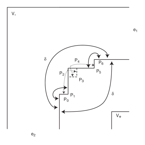
Figure 5.2. Curve system used for regeneration

We are interested in how an orthodisk system might degenerate. One such degeneration is shown in the next figure, where the points $P_{2}$, $P_{3}$, and $P_{4}$ have coalesced. The point is that the degenerating family of (pairs of) Riemann surfaces in $\Delta_{3}$ limits on (a pair of) surfaces with nodes. (We recall that a surface with nodes is a complex space where every point has a neighborhood complex isomorphic to either the disk $\{|z|<1\}$ or a pair of disks $\{(z,w)|zw=0\}$ in $\mathbb{C}^{2}$.) In the case of the surfaces corresponding to $\Omega_{Gdh}$ and $\Omega_{G^{-1}dh}$, the components of the noded surface (i.e. the regular components of the noded surface in the complement of the nodes) are difficult to observe, as the flat structures on the thrice-punctured sphere components are simply single points.

An important issue in this section is that some of our curves cross the pinching locus on the surface, i.e. the curve on the surface which is being collapsed to form the node. In particular, in the diagram, the dotted curves $\gamma_{2}$ are such curves, so their depiction in the degenerated figure is, well, degenerate: the curves connect a point and an edge.

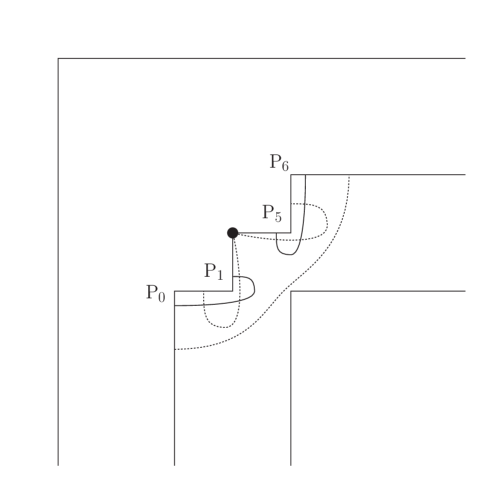
Figure 5.3. Regenerating orthodisks for the Scherk surfaces

Note that when we degenerate, we are left with the orthodisks for the surface of one lower genus, in this case that of $S_{2}$.

Our basic approach is to work backwards from this understanding of degeneration — we aim to “regenerate” the locus $\mathcal{Y}$ in $\Delta_{3}$ from the solution $X_{2}\in\Delta_{2}\subset\partial\bar{\Delta_{3}}$.

We focus on the curves $\delta$ and $\gamma_{1}$, ignoring the degenerate curve $\gamma_{2}$.

(In the general case for $\Delta_{g}$, there are $g-1$ non-degenerate curves $\{\delta,\gamma_{1},...,\gamma_{g-2}\}$), and one degenerate curve $\gamma_{g-1}$.)

We restate Lemma 5.4 in terms of the present (simpler) notation.

Lemma 5.7.

: There is a one-dimensional analytic closed locus $\mathcal{Y}\subset\overline{\Delta_{g}}$ so that both $\mathrm{ext}_{\Omega_{Gdh}}(\gamma_{i})=\mathrm{ext}_{\Omega_{G^{-1}dh}}(\gamma_{i})$ for $i=1,\dots,g-2$ and $\mathrm{ext}_{\Omega_{Gdh}}(\delta)=\mathrm{ext}_{\Omega_{G^{-1}dh}}(\delta)$ on $\mathcal{Y}$, and $\mathcal{Y}$ is proper in $\Delta_{g}$.

Proof.

We again continue with the notation for $g=3$.

As putatively defined in the statement of the lemma, $\mathcal{Y}$ would be clearly closed, and would have non-empty intersection with $\overline{\Delta_{2}}$ as $\overline{\Delta_{2}}$ contains the solution $S_{2}$ to the genus 2 problem.

We parametrize $\overline{\Delta_{3}}$ near $X_{2}$ as $\Delta_{2}\times[0,\epsilon)$ and consider the map

$$\Phi:(X,t):\Delta_{2}\times[0,\epsilon)\longrightarrow\mathbb{R}^{2}$$

given by

$$(X,t)\mapsto(\mathrm{ext}_{\Omega_{Gdh}}(\delta)-\mathrm{ext}_{\Omega_{G^{-1}dh}}(\delta),\mathrm{ext}_{\Omega_{Gdh}}(\gamma_{1})-\mathrm{ext}_{\Omega_{G^{-1}dh}}(\gamma_{1})).$$

Here, the coordinate $t$ refers to a specific choice of normalized geometric coordinate, i.e. $t=\operatorname{Im}(P_{0}P_{1}\longrightarrow P_{2}P_{3})=\operatorname{Re}(P_{3}P_{4}\longrightarrow P_{5}P_{6})$, where the periods $(P_{0}P_{1}\longrightarrow P_{2}P_{3})$ and $(P_{3}P_{4}\longrightarrow P_{5}P_{6})$ are measured on the domain $\Omega_{Gdh}$. In terms of these coordinates, we note that whenever either $t=0$, we are in a boundary stratum of $\overline{\Delta_{3}}$. The locus $\{t>0\}\subset\overline{\Delta_{3}}$ is a neighborhood in $Int(\Delta_{3})$ with $X_{2}$ in its closure.

Note that $\Phi(X_{2},0)=0$ as $X_{2}$ is reflexive.

Now, to find the locus $\mathcal{Y}$, we apply the implicit function theorem. The implicit function theorem says that if

(i) the map $\Phi$ is differentiable, and

(ii) the differential $d\Phi\bigm{|}_{T_{X_{2}}\Delta_{2}}$ is an isomorphism onto $\mathbb{R}^{2}$,

then there exists a differentiable family $\mathcal{Y}\subset\overline{\Delta_{3}}$ for which $\Phi\bigm{|}_{\mathcal{Y}}\equiv 0$.

We now prove the differentiability (condition (i)) of $\Phi$: as the locus of $\overline{\Delta_{2}}\in\widehat{\overline{\mathcal{M}}_{2}}\times\widehat{\overline{\mathcal{M}}_{2}}$ is differentiable (here $\widehat{\overline{\mathcal{M}}_{2}}$ refers to a smooth cover of the relevant neighborhood of $S_{2}\subset\overline{\mathcal{M}}_{2}$, where $\overline{\mathcal{M}}_{2}$ is the Deligne-Mostow compactification of the moduli space of curves of genus two) the theorem of Gardiner-Masur [GM] implies that $\Phi$ is differentiable, as we have been very careful to choose curves $\{\delta,\gamma_{1}\}$ which are non-degenerate in a neighborhood of $\overline{\Delta_{2}}$ near the genus two solution $S_{2}$, with both staying in a single regular component of the noded surface.

We are left to treat (ii), the invertibility of the differential $d\Phi\bigm{|}_{T_{S_{2}}\Delta_{2}}$. To show that $d\Phi\bigm{|}_{T_{S_{2}}\Delta_{2}}$ is an isomorphism, we simply prove that it has no kernel. To see this, choose a tangent direction in $T_{S_{2}}\Delta_{2}$ interpreted as a perturbation of the geometric coordinates for $S_{2}$. To be concrete, we might fix the distance between the parallel semi-infinite sides and vary the finite lengths (or periods) of the sides $P_{i}P_{i+1}$. Now, up to replacing the infinitesimal variation with its negative, one of the finite-length edges has moved into the interior of $\Omega_{Gdh}$ as in this case, with our normalization, the only edges free to move are those finite edges. Connect each of those positively moving edges with a curve system from $E_{2}P_{0}$ (and, symmetrically, $P_{4}E_{1}=P_{2g}E_{1}$). The result is a large curve system (say $\Gamma$) consisting of classes of curves from (possibly) several free homotopy classes. In addition, let $\nu$ be the associated Beltrami differential to this variation, as in section 5.2.

The flow computations in section 5 then say that this entire curve system $\Gamma$ has extremal length in $\Omega_{Gdh}$ which has decreased by an amount proportional to $|\nu|$ while the extremal length on $\Omega_{G^{-1}dh}$ has increased by an amount proportional $|\nu|$ on $\Omega_{G^{-1}dh}$. Thus, in any set of differentiable coordinates for the Teichmuller space of the surfaces in $\Delta_{2}$, the difference of coordinates for $\Omega_{Gdh}$and $\Omega_{G^{-1}dh}$ is by an amount proportional to $|\nu|$. Thus $d\Phi(\nu)\geq c|\nu|$ (for $c>0$) which proves the assertion.

To finish the proof of the lemma, we need to show that $\mathcal{Y}\bigm{|}_{\Delta_{3}}$ is an analytic submanifold of $T_{3}\times T_{3}$, where $T_{3}$ is the Teichmüller space of genus three curves: this follows on the interior of $\Delta_{3}$ from the fact that Ohtsuka’s formulas for extremal length are analytic and the map from $\Delta_{2}$ to extremal lengths has non-vanishing derivative.

This concludes the proof of Lemma 5.7 for the case $g=3$ and hence also the proof of Theorem 5.6. We have already noted that the argument is completely general, despite our having presented it in the concrete case of $S_{3}$; thus, by adding more notation, we have proven Lemma 5.7 in full generality. Naturally, this also completes the proof of Lemma 5.4.

∎

6. Embeddedness of the doubly-periodic Scherk surface with handles

In this section, we follow Karcher [11] and use the conjugate surface method from section 2.4 to prove

Proposition 6.1.

The doubly-periodic Scherk surface with handles ($S_{g}$) is embedded.

We consider a quarter of the surface, as defined by the shaded lower left quarter square of the fundamental domain of the torus, as in Figure 2.3.

Of course, this is also the part of the surface used to define the orthodisks $\Omega_{Gdh}$ and $\Omega_{G^{-1}dh}$. This surface patch, say $\Sigma_{g}$, is bounded by planar symmetry curves and one vertical end and is contained within the infinite box over a ’black’ checkerboard square. It will be sufficient to show that this patch $\Sigma_{g}$ is embedded, as the rest of the surface $S_{g}$ in space is obtained by reflecting the image $\Sigma_{g}$ of this quarter surface across vertical planes. To show that the image of the quarter surface is embedded, we prove that the conjugate surface is a graph over a convex domain; the result then follows by Krust’s Theorem in section 2.4. Thus we prove

Lemma 6.2.

The conjugate surface for $\Sigma_{g}$ is a minimal graph over a convex domain.

We apply the basic principles that straight lines and planar symmetry curves get interchanged by the operation of conjugation of minimal surfaces, and angles get preserved by this operation. Using these principles, we compute the conjugate surface for $\Sigma_{g}$.

We assert that the conjugate surface has the form depicted in the figure 6.1 and described below. The surface in the figure extends horizontally along the positive horizontal coordinate directions to infinity.

Figure 6.1. Conjugate surface patch of the doubly-periodic Scherk surface with handles

The surface patch will be bounded by two polygonal arcs in space. The first one corresponds to the $P_{1}\ldots P_{2g}$ polygonal arc of the orthodisks. As the original surface is cut orthogonally by two symmetry planes along this arc, the corresponding arc of the conjugate surface will consist of orthogonal line segments which stay in the same horizontal plane: to see this, begin by observing that the Gauss map has vertical normals at the points corresponding to the vertices of the orthodisk boundaries, hence also at the corners of the straight line segments on the conjugate surfaces. Yet where two of these segments meet, the tangent plane is tangent to both of them, hence the normal is in the unique direction normal to both; as the Gauss map is vertical, both segments must be horizontal. We conclude then that all of the straight segments must be horizontal, and hence this connected component of the boundary must lie in a horizontal plane.

Simlarly the second connected arc, this time made up of a pair of infinite arcs, is also horizontal, thus parallel to the first boundary arc.

We next claim that the two horizontal connected components of the boundary have (a pair of) parallel infinite edges as ends which lie on the same (pair of) vertical planes. To see this, consider the (pair of) cycles around the two ends $E_{1}$ and $E_{2}$: we have constructed the Weierstrass data one-forms $Gdh$ and $\frac{1}{G}dh$ so that the coordinate one-forms $(G-\frac{1}{G})dh$ and $i(G+\frac{1}{G})dh$ have purely real periods, while the coordinate one-form $dh$ has a purely imaginary period. Thus for the conjugate surface, the coordinate one-forms $(G-\frac{1}{G})dh$ and $i(G+\frac{1}{G})dh$ have purely imaginary periods, while the coordinate one-form $dh$ has a purely real period. As any representative of this cycle lifts to connect semi-infinite ends of the connected components of the boundary, and any such lift must have endpoints differing by a period, we see that the semi-infinite ends of the connected components of the boundary differ (respectively) by a purely vertical translation.

We now produce a minimal surface which spans this pair of boundary components. To do this, we first approximate the boundary by a compact boundary, then solve the corresponding Plateau problem for compact boundary values, and then finally take a limit. More precisely, consider a boundary formed from the boundary arcs described above by introducing vertical segments $\Gamma_{b,1}$ and $\Gamma_{b,2}$ connecting the two pairs of parallel semi-infinite boundary edges at distance $b$ from the (image of the) point $P_{g}$. This boundary is now compact and projects injectively onto a rectangle boundary by using the projection in the direction of the ’diagonal’ vector $(1,1,0)$.

This corresponding boundary problem has a classical Plateau solution which is unique and a graph over the plane orthogonal to $(1,1,0)$ by Radó’s theorem. We now look at a sequence of such Plateau solutions for increasing values of $b\to\infty$. Using solutions for smaller values of $b$ as barriers for the solutions corresponding to the larger values of $b$, by the maximum principle we see that the solutions $S_{g,b}^{*}$ form an increasing sequence of graphs. To show that this sequence actually converges, it suffices to show that the intersections $A_{b}$ of the family of surfaces with the vertical plane $\Pi$ passing through $P_{g}$ and $V_{\pm}$ lie in a single compact set. To see this, we consider a pair of (quarters of) Scherk surfaces (conjugate to $S_{0}$), each of whose boundary components consist of an infinite $L$ and a vertical translate of that $L$ by the same amount as for a conjugate surface for $S_{g}$. The first such conjugate Scherk passe through the point $P_{g}$, while the second is displaced to pass through the points $V_{\pm}$. This pair of boundary arcs lie to the other side of the boundary arcs of $S_{g}$ in the respective horizontal planes. Thus, this pair of surfaces meets the plane $\Pi$ in a pair of arcs, which, by the maximum principle lie to either side of the arcs $A_{b}$ on the strip of $\Pi$ between our fixed pair of horizontal planes.

Thus, by Harnack, the approximate solutions $S_{g,b}^{*}$ converge to a solution $S_{g}^{*}$ for the infinite boundary problem; as the approximate solutions are all graphs and minimal, the limit $S_{g}^{*}$ is also a graph (here convergence of the graphed functions $u_{b}$ in $C^{0}$ implies their convergence in $C^{1}$ by standard elliptic theory, hence to a graph). Then, by Krust’s theorem, the conjugate patch to that limit graph is also a graph, and since that conjugate patch is a fundamental piece of our surface $S_{g}$, we see that $S_{g}$ is embedded. ∎

References

- [1] Frank Baginski and Valerio Ramos-Batista. Solving period problems for minimal surfaces with the support function. preprint, 2008.
- [2] E. Boix and M. Wohlgemuth. Numerical results on embedded minimal surfaces of finite total curvature. In perpetual preparation.
- [3] P. Connor and M. Weber. Doubly periodic minimal surfaces with parallel ends. Preprint, 2009.
- [4] U. Dierkes, S. Hildebrandt, A. Küster, and O. Wohlrab. Minimal Surfaces I. Grundlehren der mathematischen Wissenschaften 295. Springer-Verlag, 1992. MR1215267, Zbl 0777.53012.
- [5] C. Douglas. Doubly Periodic Minimal Surfaces of Genus 1. PhD thesis, Rice University, Houston, 2008.
- [6] A. Fathi, F. Laudenbach, and V. Poenaru. Traveaux de Thurston sur les Surfaces. Société Mathématique de France. Astérisque.
- [7] F.P. Gardiner. Teichmuller Theory and Quadratic Differentials. Wiley Interscience, New York, 1987.
- [8] F.P. Gardiner and H. Masur. Extremal length geometry of teichmüller space. Complex Analysis and its Applications, 16:209–237, 1991.
- [9] J. Hubbard and H. Masur. Quadratic differentials and foliations. Acta Math., 142:221–274, 1979.
- [10] H. Jenkins. On the existence of certain general extremal metrics. Ann. of Math., 66:440–453, 1957. MR0190811 , Zbl 171.08301.
- [11] H. Karcher. Embedded minimal surfaces derived from Scherk’s examples. Manuscripta Math., 62:83–114, 1988. MR0958255, Zbl 658.53006.
- [12] H. Karcher. Construction of minimal surfaces. Surveys in Geometry, pages 1–96, 1989. University of Tokyo, 1989, and Lecture Notes No. 12, SFB256, Bonn, 1989.
- [13] S. Kerckhoff. The asymptotic geometry of teichmüller space. Topology, 19:23–41, 1980.
- [14] H. B. Lawson, Jr. Lectures on Minimal Submanifolds. Publish or Perish Press, Berkeley, 1980. MR0576752, Zbl 0434.53006.
- [15] H. Lazard-Holly and W. H. Meeks III. The classification of embedded doubly–periodic minimal surfaces of genus zero. Invent. Math., 143:1–27, 2001. MR1802791, Zbl 992.18190.
- [16] W. H. Meeks III and H. Rosenberg. The geometry, topology, and existence of doubly periodic minimal surfaces. C. R. Acad. Sci. Paris, 306:605–609, 1988. Research Announcement.
- [17] W. H. Meeks III and H. Rosenberg. The global theory of doubly periodic minimal surfaces. Invent. Math., 97:351–379, 1989. MR1001845, Zbl 676.53068.
- [18] M. Ohtsuka. Dirichlet Problem, Extremal Length and Prime Ends. Van Nostrand Reinhold, New York, 1970.
- [19] R. Osserman. A Survey of Minimal Surfaces. Dover Publications, New York, 2nd edition, 1986. MR0852409, Zbl 0209.52901.
- [20] J. Pérez, M. Rodríguez, and M. Traizet. The classification of doubly periodic minimal tori with parallel ends. Journal of Diff. Geometry, 69(3):523–577, 2007. MR2170278, Zbl pre05004289.
- [21] H. F. Scherk. Bemerkungen über die kleinste Fläche innerhalb gegebener Grenzen. J. R. Angew. Math., 13:185–208, 1835. ERAM 013.0481cj.
- [22] K. Strebel. Quadratic Differentials. Springer, Berlin, 1984.
- [23] E. Thayer. Complete Minimal Surfaces in Euclidean 3-Space. PhD thesis, University of Massachusetts at Amherst, 1994.
- [24] M. Traizet. An embedded minimal surface with no symmetries. J. Differential Geometry, 60(1):103–153, 2002. MR1924593, Zbl 1054.53014.
- [25] M. Traizet. Adding handles to Riemann minimal examples. J. Differential Geom., 79:243–275, 2008. MR2420019, Zbl pre05294962.
- [26] M. Wohlgemuth W. Rossman, E. Thayer. Embedded, doubly periodic minimal surfaces. Exp. Math., 9(2):197–219, 2000.
- [27] M. Weber, D. Hoffman, and M. Wolf. An embedded genus-one helicoid. Ann. of Math., 169(2):347–448, 2009. MR2480608.
- [28] M. Weber and M. Wolf. Minimal surfaces of least total curvature and moduli spaces of plane polygonal arcs. Geom. Funct. Anal., 8:1129–1170, 1998. MR1664793, Zbl 0954.53007.
- [29] M. Weber and M. Wolf. Teichmüller theory and handle addition for minimal surfaces. Ann. of Math., 156:713–795, 2002. MR1954234, Zbl 1028.53009.
- [30] F. Wei. Some existence and uniqueness theorems for doubly periodic minimal surfaces. Invent. Math., 109:113–136, 1992. MR1168368, Zbl 773.53005.
- [31] M. Wohlgemuth. Higher genus minimal surfaces by growing handles out of a catenoid. Manuscripta Math., 70:397–428, 1991.
- [32] M. Wohlgemuth. Vollständige Minimalflächen höheren Geschlechts und endlicher Totalkrümmung. PhD thesis, University of Bonn, April 1993.
- [33] M. Wohlgemuth. Higher genus minimal surfaces of finite total curvature. Preprint, 1994.
- [34] Michael Wolf. On realizing measured foliations via quadratic differentials of harmonic maps to -trees. J. Anal. Math., 68:107–120, 1996.