Anomalies, gauge field topology, and the lattice

Abstract

Motivated by the connection between gauge field topology and the axial anomaly in fermion currents, I suggest that the fourth power of the naive Dirac operator can provide a natural method to define a local lattice measure of topological charge. For smooth gauge fields this reduces to the usual topological density. For typical gauge field configurations in a numerical simulation, however, quantum fluctuations dominate, and the sum of this density over the system does not generally give an integer winding. On cooling with respect to the Wilson gauge action, instanton like structures do emerge. As cooling proceeds, these objects tend shrink and finally “fall through the lattice.” Modifying the action can block the shrinking at the expense of a loss of reflection positivity. The cooling procedure is highly sensitive to the details of the initial steps, suggesting that quantum fluctuations induce a small but fundamental ambiguity in the definition of topological susceptibility.

1 Introduction

One of the great theoretical advances of the 1970’s was the understanding of the connection between gauge field topology and the axial anomaly [1]. One consequence of this resolution was the realization that a CP violating parameter can be introduced into the strong interactions. In the context of unification, this raised the puzzle as to why such a parameter seems to be absent or at least experimentally quite small. For a recent review, see Ref. [2]. Fujikawa [3] provided a simple interpretation of these phenomena in terms of the properties of the fermionic measure in the path integral. Indeed, this approach provides an elegant derivation of the index theorem relating the gauge field topology to the number of zero modes of the Dirac operator. Witten [4] used large gauge group ideas and effective Lagrangian techniques to explore the behavior of the theory on this CP violating parameter.

There is a long history of attempts to understand this physics in the context of lattice gauge theory, now the primary tool for understanding non-perturbative field theory. The idea of continuity in space time, crucial to topology, is lost on the lattice. With gauge field space being a direct product of group elements on discrete space time links, it is always possible to continuously and locally deform fields between arbitrary configurations. This issue can be mollified by placing rather strong smoothness restrictions on the differences of fields at nearby locations, thereby giving rise to a unique continuum interpolation [5]. However these restrictions can be shown to mutilate fundamental properties such as reflection positivity [6]. Note that many current simulations use discretizations that violate this condition; the point is not that these are unacceptable in practice, but rather that any acceptable rigorous definition of winding number must not exclude formulations that do satisfy this axiom.

Although the issues are quite old [7], they continue to generate many recent discussions, i.e. Refs. [8, 9, 10, 11]. Thus I return to this topic with a new definition of topology based on a generalization of the Fujikawa picture, wherein the trace of $\gamma_{5}$ times the fourth power of the Dirac operator contains a contribution proportional to the topological charge. The motivation is to provide a definition that is particularly closely tied to the fermion operator and the index theorem.

The specific lattice operator I consider is a sum over loops running around fundamental hypercubes. This provides a local definition of topological charge that for smooth fields agrees with the continuum definition. On rough fields typical in a simulation, however, it is not generally integer valued. It does become so after a cooling procedure to remove the short distance fluctuations.

Throughout I treat the fermionic fields merely as a probe of the gluon fields. While one could extend the discussion to include dynamical fermions, in this paper the quarks play no role in the gluon dynamics. Another example of using powers of the Dirac operator to probe gluonic fields appears in [12]. References [13, 14, 15] go further and suggest using a Dirac operator itself to dynamically generate the gluon interactions.

Section 2 reviews the argument of Fujikawa relating the anomaly to the fermionic measure. Section 3 extends this review to a simple derivation of the index theorem for smooth fields. Then Section 4 introduces the specific lattice operator under discussion and presents simulations showing that quantum fluctuations blur any discrete topological structures. Section 5 shows that such structures do become evident under the process of cooling, also sometimes referred to as smearing, to smooth out short distance fluctuations. Here I also discuss the eventual decay of the instanton structures as they shrink and fall through the lattice due to lattice artifacts. Section 7 discusses the properties imposed on this operator by reflection positivity and the importance of the contact term present in the correlators of the density operator. Section 8 returns to the cooling process and discusses ambiguities in the topological charge due to a chaotic nature of the initial cooling steps. This raises the question of whether topological susceptibility is actually a physical observable, or is there a fundamental uncertainty in its definition. I illustrate the ideas with simulations based on pure $SU(2)$ lattice gauge theory with the standard Wilson gauge action with coupling $\beta$ [16]. The final section summarizes the basic ideas of the paper.

2 Fermions and the anomaly

The chiral anomaly is associated with a flavor singlet transformation on the fermion fields

$$\psi\rightarrow e^{i\gamma_{5}\phi/2}\psi$$ (1)

$$\overline{\psi}\rightarrow\overline{\psi}e^{i\gamma_{5}\phi/2}.$$ (2)

(3)

Here $\psi$ represents the quark fields and has implicit spinor and flavor indices. Consider the naive kinetic term for massless quarks

$$\overline{\psi}\hbox to0.0pt{\hbox to8.55695pt{\hfil/\hfil}\hss}D\psi=\overline{\psi}\gamma_{\mu}(\partial_{\mu}+ieA_{\mu})\psi.$$ (4)

Because $\gamma_{5}$ anti-commutes with the anti-hermitian operator $\hbox to0.0pt{\hbox to8.55695pt{\hfil/\hfil}\hss}D$, massless QCD naively is invariant under the above transformation. The essence of the chiral anomaly is that any valid regulator must break this symmetry and leave behind physical consequences.

A particularly elegant way to understand the connection between the anomaly and the index theorem is due to Fujikawa [3], who mapped the problem onto the fermionic measure in the path integral. Under the above transformation the fermionic measure changes by

$$d\psi\ d\overline{\psi}\rightarrow\det(e^{i\gamma_{5}\phi})d\psi\ d\overline{\psi}$$ (5)

Using the matrix relation $\det A=\exp({\rm Tr}\log(A))$, this reduces to

$$d\psi\ d\overline{\psi}\rightarrow(e^{i\phi{\rm Tr}\gamma_{5}})d\psi\ d\overline{\psi}.$$ (6)

If one could say that ${\rm Tr}\gamma_{5}=0$, the measure would be invariant under this transformation.

The crucial result is that any valid regulator must modify the naive tracelessness of $\gamma_{5}$. The details of how this works depends on the specifics of the regulator, but basically the issue involves reconciling the infinity of the dimension of space time with the naive relation ${\rm Tr}\gamma_{5}=0$. A convenient approach is to use the fermion operator itself to regulate the theory and define

$${\rm Tr}\gamma_{5}\equiv\lim_{\Lambda\rightarrow\infty}\gamma_{5}e^{{\hbox to0.0pt{\hbox to5.98985pt{\hfil/\hfil}\hss}D}^{2}/\Lambda^{2}}.$$ (7)

With this it is natural to expand in the eigenvectors of $\hbox to0.0pt{\hbox to8.55695pt{\hfil/\hfil}\hss}D$

$$\hbox to0.0pt{\hbox to8.55695pt{\hfil/\hfil}\hss}D|\psi_{i}\rangle=\lambda_{i}|\psi_{i}\rangle$$ (8)

and define

$${\rm Tr}\gamma_{5}=\lim_{\Lambda\rightarrow\infty}\sum_{i}\langle\psi_{i}|\gamma_{5}|\psi_{i}\rangle e^{\lambda_{i}^{2}/\Lambda^{2}}$$ (9)

Since $D$ is anti-hermitian, its eigenvalues fall on the imaginary axis. The eigenvectors divide into two classes, those with non-zero $\lambda_{i}$ and zero modes with $\lambda_{i}=0$. The former always appear in complex conjugate pairs since $[\hbox to0.0pt{\hbox to8.55695pt{\hfil/\hfil}\hss}D,\gamma_{5}]_{+}=0$ implies $\hbox to0.0pt{\hbox to8.55695pt{\hfil/\hfil}\hss}D\gamma_{5}|\psi_{i}\rangle=-\lambda_{i}\gamma_{5}|\psi\rangle$. Since $|\psi_{i}\rangle$ and $\gamma_{5}|\psi_{i}\rangle$ have different eigenvalues, whenever $\lambda_{i}\neq 0$ they are orthogonal

$$\langle\psi_{i}|\gamma_{5}|\psi_{i}\rangle=0.$$ (10)

Such states do not contribute to the above sum for the trace of $\gamma_{5}$. Indeed, this trace only receives contributions from the set of zero modes of the Dirac operator. Restricted to the space spanned by this set, $\hbox to0.0pt{\hbox to8.55695pt{\hfil/\hfil}\hss}D$ and $\gamma_{5}$ commute and thus can be simultaneously diagonalized. Let $n_{+}(n_{-})$ be the number of zero modes with eigenvalue $+1(-1)$ for $\gamma_{5}$. Now recall the well known index theorem that the net winding number $\nu$ of the gauge field is given by the difference of positive and negative chirality zero modes of the Dirac equation.

$${\rm Tr}\gamma_{5}=n_{+}-n_{-}=\nu.$$ (11)

Rather than being traceless, the regulated $\gamma_{5}$ in the path integral is actually an operator depending on the gauge field. On making the chiral transformation in Eq. (3), the path integral picks up a factor $e^{i\nu\phi}$.

Now consider the theory with a non-vanishing quark mass term $m\overline{\psi}\psi$. Under the rotation of Eq. (3), this is not invariant but becomes

$$m\overline{\psi}\psi\rightarrow m(\cos(\phi)\overline{\psi}\psi+i\sin(\phi)\overline{\psi}\gamma_{5}\psi)$$ (12)

Since the transformation is naively a change of variables, one might expect a theory with a mass term of the form of the right hand side of Eq. (12) would give the same physics. However this is incorrect since by the above discussion this change reweights configurations of non-trivial winding. This gives a physically inequivalent theory. In particular, since the term involving $i\overline{\psi}\gamma_{5}\psi$ is not invariant under CP, this new theory does not respect this symmetry.

Here I have given the same rotation to each species. With $N_{f}$ flavors of fermion, each contributes equally to the measure, thus the factor appearing in the path integral is actually $e^{iN_{f}\nu\phi}$ and physics is periodic in $\phi$ with period $2\pi/N_{f}$. This leads to the more conventional definition of the angle $\Theta=N_{f}\phi$, in which physics is periodic with period $2\pi$. One might ask where did the opposite chirality states go. The are in some sense “beyond the cutoff,” having been suppressed by the factor $e^{\hbox to0.0pt{\hbox to5.98985pt{\hfil/\hfil}\hss}D^{2}/\Lambda^{2}}$.

3 The index theorem

This approach leads to a simple derivation of the index theorem. Assume the gauge fields are smooth and differentiable. Writing out the square of the Dirac operator gives

$${\hbox to0.0pt{\hbox to8.55695pt{\hfil/\hfil}\hss}D}^{2}=\partial^{2}-g^{2}A^{2}+2igA_{\mu}\partial_{\mu}+ig(\partial_{\mu}A_{\mu})-{g\over 2}\sigma_{\mu\nu}F_{\mu\nu}$$ (13)

where $[\gamma_{\mu},\gamma_{\nu}]=2i\sigma_{\mu\nu}$. Expanding ${\rm Tr}\gamma_{5}e^{{\hbox to0.0pt{\hbox to5.98985pt{\hfil/\hfil}\hss}D}^{2}/\Lambda^{2}}$ in powers of the gauge field, the first non-vanishing term is contained in the fourth power of the Dirac operator. This involves two powers of the sigma matrices

$$\nu={\rm Tr}\gamma_{5}e^{{\hbox to0.0pt{\hbox to5.98985pt{\hfil/\hfil}\hss}D}^{2}/\Lambda^{2}}={1\over 2\Lambda^{4}}{\rm Tr}_{x,c}e^{\partial^{2}/\Lambda^{2}}\epsilon_{\mu\nu\rho\sigma}F_{\mu\nu}F_{\rho\sigma}$$ (14)

where ${\rm Tr}_{x,c}$ refers to the trace over space and color, the trace over the spinor index having been done to give a factor of 4. It is the trace over the space index that will give a divergent factor removing the $\Lambda^{-4}$ prefactor. Higher order terms go to zero rapidly enough with $\Lambda$ to be ignored.

The factor $e^{\partial^{2}/\Lambda^{2}}$ serves to mollify traces over position space. Consider some function $f(x)$ as representing a a diagonal matrix in position space $M(x,x^{\prime})=f(x)\delta(x-x^{\prime})$ The formal trace would be ${\rm Tr}M=\int dxM(x,x)$, but this diverges since it involves a delta function of zero. Writing the delta function in terms of its Fourier transform

$$e^{\partial^{2}/\Lambda^{2}}\delta(x-x^{\prime})=\int{d^{4}p\over(2\pi)^{4}}e^{ip\cdot(x-x^{\prime})}e^{-p^{2}/\Lambda^{2}}={\Lambda^{4}\over 16\pi^{2}}e^{-(x-x^{\prime})^{2}\Lambda^{2}/4}$$ (15)

shows how this “heat kernel” spreads the delta function. This regulates the desired trace

$${\rm Tr}_{x}f(x)\equiv{\Lambda^{4}\over 16\pi^{2}}\int d^{4}xf(x).$$ (16)

Using this to remove the spatial trace in the above gives the well known relation

$$\nu={1\over 32\pi^{2}}{\rm Tr}_{c}\int d^{4}x\epsilon_{\mu\nu\rho\sigma}F_{\mu\nu}F_{\rho\sigma}={1\over 16\pi^{2}}{\rm Tr}_{c}\int d^{4}xF_{\mu\nu}\tilde{F}_{\mu\nu}$$ (17)

where $\tilde{F}_{\mu\nu}={1\over 2}\epsilon_{\mu\nu\rho\sigma}F_{\rho\sigma}$.

4 A local lattice operator for topology

The previous argument showed that the fourth power of the Dirac operator has a close connection to topological charge. To obtain something with non-vanishing trace, one must multiply $\gamma_{5}$ by each of the four space-time gamma matrices. In the above discussion, these factors were provided by the square of the $\sigma_{\mu\nu}F_{\mu\nu}$ term in Eq. (13).

In a lattice formulation, one obtains gamma matrix factors for each fermion hopping term, and thus can obtain the necessary factors by hopping once in each of the four directions. This suggests one should study contributions to lattice operators of the form ${\rm Tr}\gamma_{5}{\hbox to0.0pt{\hbox to8.55695pt{\hfil/\hfil}\hss}D}^{4}$. This leaves open what lattice Dirac operator to use. With an overlap formulation [17], calculating ${\rm Tr}\ \gamma_{5}e^{\hbox to0.0pt{\hbox to5.98985pt{\hfil/\hfil}\hss}D^{2}/\Lambda^{2}}$ amounts to a simple counting of zero modes. However the overlap operator is rather tedious to compute. With the naive lattice discretization, the fermion operator just involves nearest neighbor hops accompanied with the corresponding gamma matrices. For the free theory in momentum space this is

$$\hbox to0.0pt{\hbox to8.55695pt{\hfil/\hfil}\hss}D(p)=\sum_{\mu}i\gamma_{\mu}\sin(p_{\mu}).$$ (18)

In position space this gives a factor of $\pm i\gamma_{\mu}/2$ for hops in the $\pm\mu$ direction. With gauge fields present, the hop is accompanied by the corresponding gauge link field $U$.

Of course the naive fermion action involves doublers, but for the above counting one could imagine removing this with a simple numerical factor. A complication here is that the various doublers have different chiralities. When some component of momentum is near $\pi$, the slope of $\sin(p_{\mu})$ in that direction brings in a minus sign, and the doubler uses an opposite sign for that particular gamma matrix. Half the doublers use the opposite sign for $\gamma_{5}$ and thus the naive $\gamma_{5}$ is actually a non-singlet operator. As such, the corresponding chiral symmetry is not anomalous and ${\rm Tr}\ \gamma_{5}e^{\hbox to0.0pt{\hbox to5.98985pt{\hfil/\hfil}\hss}D^{2}/\Lambda^{2}}$ explicitly vanishes.

The simplicity of the naive Dirac operator makes it worth trying to get around this and consider a new chiral matrix that is closer to a flavor singlet. In momentum space for free fermions I define

$$\Gamma_{5}=\gamma_{5}\prod_{\mu}\cos(p_{\mu}).$$ (19)

Whenever a component of the momentum is near $\pi$, this introduces a minus sign to compensate for the effective Dirac matrix used by the doubler.

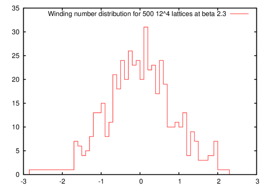
Figure 1: The distribution of the lattice winding number defined in the text on a set of 500 $SU(2)$ lattices of size $12^{4}$ at $\beta=2.3$.

Going back to position space, the factors of $\cos(p_{\mu})$ are represented by averaging hoppings in the $\pm\mu$ direction. Reintroduce the gauge fields with insertions of the link variables into these hoppings. Since the order of the hoppings should not matter, consider the average over all such. Thus our candidate for the anomalous flavor singlet chiral matrix involves taking $\gamma_{5}$ augmented by a hop in each of the four space time directions. These hops are summed over positive and negative directions and all orderings. The result is that $\Gamma_{5}$ is a non-local operator connecting opposite corners of lattice hypercubes.

This suggests the candidate operator for measuring topology

$$q\propto{\rm Tr}\ \Gamma_{5}{\hbox to0.0pt{\hbox to8.55695pt{\hfil/\hfil}\hss}D}^{4}$$ (20)

with ${\hbox to0.0pt{\hbox to8.55695pt{\hfil/\hfil}\hss}D}$ being the naive lattice fermion operator. Each term in this construction involves eight hoppings, four from the $\Gamma_{5}$ factor and one from each factor of ${\hbox to0.0pt{\hbox to8.55695pt{\hfil/\hfil}\hss}D}$. Because the trace forces the hops to return to the starting site, this quantity is gauge invariant.

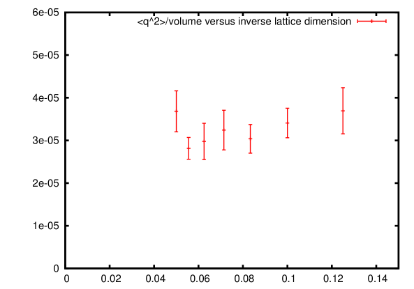
Figure 2: The average topological charge squared divided by the system volume versus the linear lattice size at $\beta=2.3$ for lattices of size $8^{4}$ to $20^{4}$.

So the final operator I wish to construct is defined on hypercubes. For any given hypercube, consider all 16 directed hyper-diagonals. For each diagonal, sum over all four-hop paths along hypercube edges from one end to the other followed by all four-hop paths back to the starting site. Finally given any particular path, assign a sign corresponding to the parity of the permutation of the initial four hops. This is a sum over $24^{2}*16$ Wilson loops.

In practice one need not actually calculate all these loops individually. Accumulating the forward paths into two matrices, one being the sum and one being the sum with the sign factor included, the desired sum of loops is immediately found from the product of the first sum times the adjoint of the second. Also, each diagonal need be calculated only in one direction since the reverse is equivalent.

To normalize this construction, consider small smooth fields ask that the sum give the classical winding number

$$q\rightarrow\nu={1\over 16\pi^{2}}\int d^{4}x{\rm Tr}_{c}F\tilde{F}$$ (21)

where ${\rm Tr}_{c}$ refers to a trace over color matrices. The result is that one should multiply the above sum over Wilson loops by a factor of ${1\over 3*2^{10}\pi^{2}}$. Note that this is independent of the size of the gauge group.

Because the lattice fields tend to be quite rough, this quantity has no need to peak at integer values. In Fig. (1) I show the distribution of $q$ over a set of 500 independent gauge configurations with gauge group $SU(2)$ at a coupling $\beta=2.3$ on a $12^{4}$ site lattice.

The average value of $q^{2}$ should scale with the lattice volume. In Fig. (2) I show this quantity calculated at $\beta=2.3$ on lattices of size from $8^{4}$ to $20^{4}$. On the $18^{4}$ lattice, the topological susceptibility per unit volume in lattice units is $(2.8\pm 0.25)\times 10^{-5}$.

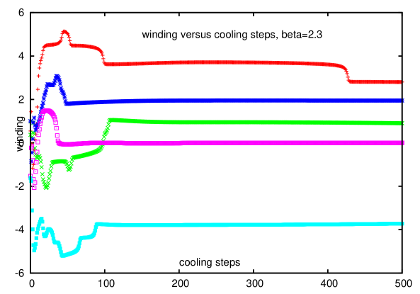
Figure 3: The winding number as a function of cooling steps for a set of 5 lattices of size $16^{4}$ at $\beta=2.3$. Note how it settles into approximately integer values with occasional jumps between different windings.

5 Cooling

It has been known for some time that to expose topological structures in lattice configurations requires some cooling procedure to remove short distance roughness [7]. A particularly simple process is to loop over the lattice in a checkerboard manner and replace each link with the group element which minimizes the total action of the six plaquettes attached to that link. This can be modified by over or under relaxation, which I will discuss later. Such processes monotonically decrease the total action. In Fig. (3) I show how the above winding number evolves for 5 independent $16^{4}$ site lattices at $\beta=2.3$. Note how the winding tends to fall into discrete values, with jumps between them as the cooling proceeds further. Indeed, with long enough cooling the winding always appears to eventually drop to zero. Also note that the discrete values tend to be somewhat below integers; this is presumably a lattice artifact which becomes more severe at higher winding number. Finally, note that the initial relaxation steps appear to be rather chaotic.

The discrete levels of non-trivial winding can also be seen directly in the total action. In Fig. (4) I show the evolution of the action for cooling the same 5 configurations. The classical instanton result for the lattice action is that these levels should appear at a multiple of $2\pi^{2}$, which seems to be well satisfied.

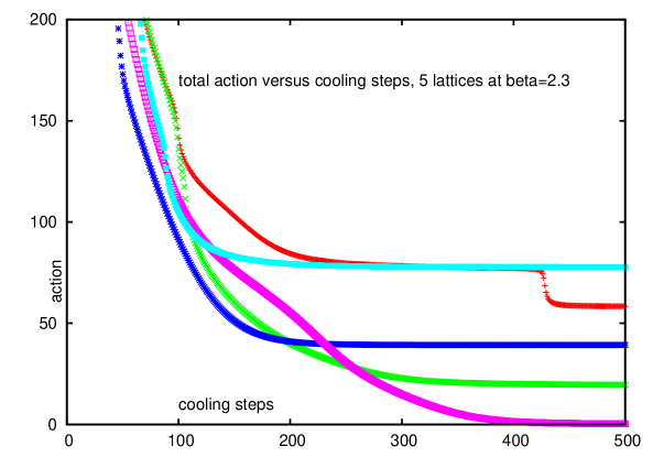
Figure 4: The total Wilson action as a function of cooling steps for a set of 5 lattices of size $16^{4}$ at $\beta=2.3$. The level portions occur at approximate multiples of the classical instanton action of $2\pi^{2}$. These are the same lattices as in Fig. 3.

To better understand the jumps between levels, it is interesting to look at the maximum local action associated with a single link. This is plotted in Fig. (5) for the same 5 configurations. Note the evident peaks at the points where the winding jumps. Although the total action decreases monotonically, this is not in general true locally. This is because the instanton like structures can decrease in size with their action being concentrated in a smaller region. Eventually the structures drop down to the lattice size and collapse “through the lattice.” This shrinking of topological structures is a lattice artifact. In particular, the classical continuum theory is conformally invariant with an instanton action independent of size.

The height of the observed peaks is approximately 0.2. As each link involves six plaquettes, one can stop the decay by forbidding each plaquette to be larger than one sixth of that, or something like 0.03. This compares well with the “admissibility condition” of Luscher [5] which, when obeyed, allows the gauge fields to be uniquely continued between lattice sites to form a smooth continuum field. Unfortunately, such a condition has been shown to be inconsistent with reflection positivity [6].

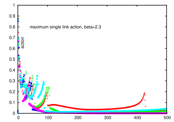
Figure 5: The maximum Wilson action associated with a single lattice link as a function of cooling steps for a set of 5 lattices of size $16^{4}$ at $\beta=2.3$. The peaks represent “instantons” falling through the lattice.

6 The decay of an instanton

It is perhaps interesting to study the way winding number disappears with cooling in a more controlled manner. To do this I construct a configuration that quickly settles into a classical instanton and then watch its evolution under cooling. For an initial state I start with all links unity and then do a gauge transformation with gauge function

$$h(x_{\mu})={x_{0}+i\vec{x}\cdot\vec{\sigma}\over\sqrt{x_{0}^{2}+\vec{x}^{2}}}$$ (22)

Here I define $x_{\mu}$ as the distance of a given site from the center of a hypercube at the center of the lattice. Since this is just a gauge transformation, this leaves a configuration which still has vanishing action. As one moves away from the lattice center the links approach unity everywhere except for those links crossing the boundary. I now make the action non-trivial by replacing all links that cross the boundary with unity. With this starting configuration, I then apply the cooling process.

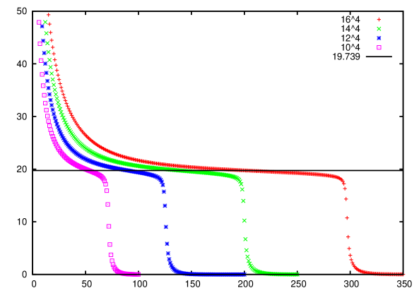
Figure 6: The evolution of the action under cooling with the initial configuration described in the text on lattices sizes from $10^{4}$ to $16^{4}$. The classical instanton action is marked by the horizontal line.

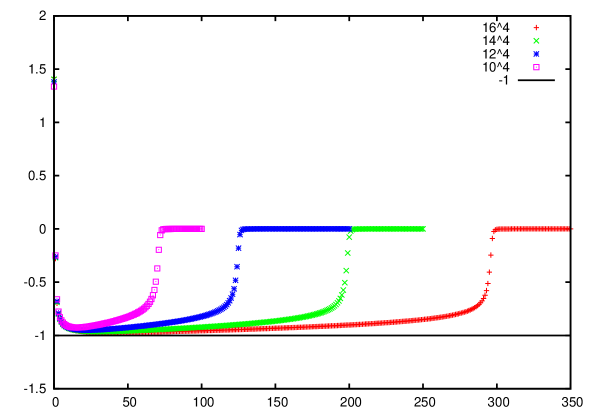
Figure 7: The evolution of the winding number under cooling with the initial configurations described in the text. The classical anti-instanton winding is marked by the horizontal line.

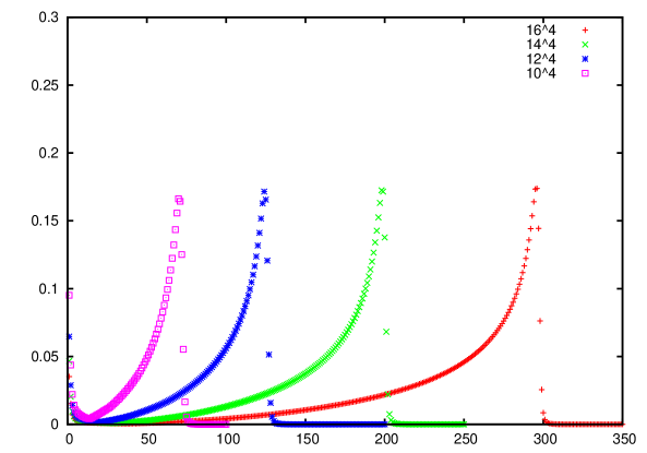
Figure 8: The evolution of the largest action associated with a single link under cooling with the initial configurations described in the text. The peak represents the instanton collapsing through the lattice.

In Fig. (6) I show the evolution of the action for such configurations under cooling for various size lattices. In the figure I also indicate $2\pi^{2}$, which is the action of a smooth classical instanton. Note how the action quickly relaxes to this value, then gradually decreases while the instanton shrinks and finally drops to zero. The number of steps for this collapse increases with lattice size because the initial topology becomes spread over a larger region.

Fig. (7) shows the topological winding number during this process. After the roughness at the boundary smooths out, this quickly drops to near $-1$, indicating that the construction actually gives rise to an anti-instanton. The evolution then remains near unity until the time of the action drop.

Finally, in Fig. (8) I plot the maximum action associated with a single link during this cooling. As the instanton becomes smaller, the action is more concentrated and a peak appears just before the collapse. This is an analogous peak to those appearing in the cooling of equilibrated lattices as in Fig. (5).

7 Reflection positivity and topological charge

Reference [18] pointed out an interesting property that any local definition of topological charge must have. Because the underlying operator $F\tilde{F}$ is odd under time reversal, reflection positivity requires its correlator with itself at non-vanishing separation to be negative. On the other hand, the square of its integral over space time must be positive. Therefore in calculating the square of the topological charge, there is a subtle cancellation between the positive contact term and the negative contribution from correlations at non-vanishing separations. This is a somewhat non-intuitive result that led Horvath [19, 20] to interpret the typical vacuum state in terms of a highly crumpled field structure. The separation of the topological charge into contact and non-contact pieces is shown in Fig. (9).

The negative nature of the correlators of topological charge is a statement about their average. It is, however, possible for fluctuations to give these correlators positive contributions on a configuration by configuration basis. In Fig. (10) I plot the evolution of the non-contact term over a sequence of 105 configurations on a $16^{4}$ lattice at $\beta=2.3$.

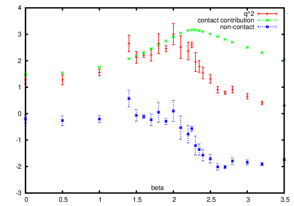
Figure 9: The average topological charge squared for $SU(2)$ on a $16^{4}$ lattice versus $\beta$ plotted along with the contact and non-contact contributions separated. As required by reflection positivity, the non-contact contribution is negative.

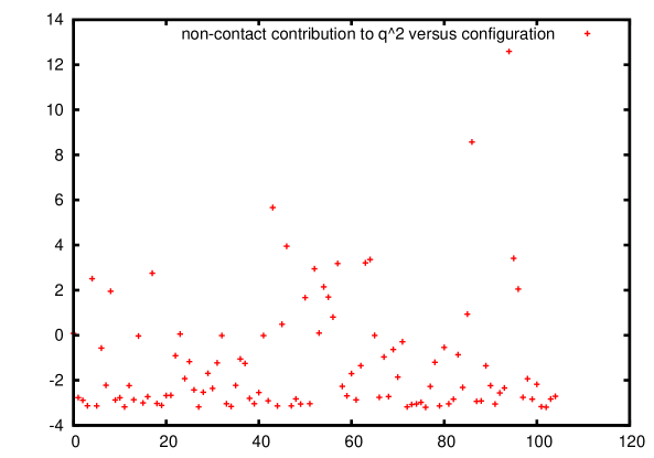
Figure 10: The non-contact contribution to $q^{2}$ over a sequence of 105 gauge configurations. Although the average is negative as required, there are large fluctuations giving a positive contribution from specific configurations. This figure is using $SU(2)$ on a $16^{4}$ lattice at $\beta=2.3$.

The definition of charge density used here is highly local, involving single hypercubes. As a consequence, the negative nature of the correlation starts immediately for adjacent hypercubes. In Fig. (11) I show the correlation between the charge density on hypercubes separated along an axis by one and two lattice units.

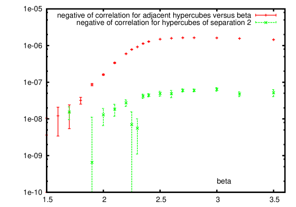
Figure 11: The negative of the correlation of winding number density between adjacent hypercubes and hypercubes of on axis separation two plotted as a function of the coupling beta. As required by reflection positivity, the correlation is negative. This plot is for $SU(2)$ gauge theory on a $16^{4}$ lattice.

The cooling process discussed in Section 5 smooths out the fields in a way that does not maintain the negative nature of this correlation. Indeed, during the cooling process the non-contact part quickly comes to dominate the total contribution to the square of the topological charge.

At long distances the correlator between charge densities should fall exponentially with the mass of the lightest singlet pseudoscalar meson. For pure gauge fields, this is a glueball, but with quarks of physical masses present this will be the eta prime meson. (More precisely, with physical quark masses the eta prime decays into three pions which give the ultimate asymptotic behavior; I ignore this complication here.) Thus measuring this correlator provides a route to the eta prime mass which replaces the complexity of separating connected and disconnected quark diagrams with potentially large statistical fluctuations.

8 Sensitivity to initial conditions

The charge operator defined above does not give an integer value on a typical gauge configuration. Indeed, some cooling is necessary to remove short distance fluctuations before discrete winding numbers are observed. Empirically with enough cooling any $SU(2)$ gauge configuration appears to eventually decay to a state of zero action, gauge equivalent to the vacuum. This is not in general true for larger gauge groups. Indeed, for $SU(N)$ with $N\geq 5$ there exist non-trivial gauge configurations that are stable minima under arbitrary small variations of the fields but have nothing to do with topology. For example, consider all links to be unity except for a few isolated links with values in the group center nearest the identity, i.e. of form $e^{\pm 2\pi i/N}$. When $N$ is five or more, small deviations from these center elements will raise the action. Such configurations do not involve gauge field winding, but are sufficient to give stable non-minimal action states.

Since topological configurations appear to always eventually cool to triviality, using cooling to define winding number requires an arbitrary selection for cooling time. Modifying the Wilson action can prevent the winding decay. As discussed earlier, on forbidding the lattice action on any given plaquette from becoming larger than a small enough number, the peaks seen in Fig (5) cannot be crossed. Such a condition, however, violates reflection positivity and arbitrarily selects a special instanton size where the action is minimum.

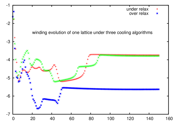
Figure 12: The topological charge evolution for three different cooling algorithms on a single $\beta=2.3$ lattice configuration for $SU(2)$ on a $16^{4}$ lattice.

Cooling time is not the only issue here. While integer winding does not appear before cooling, note from Fig. (3) that the initial cooling stages seem quite chaotic. This raises the question of whether the discrete stages reached after some cooling might depend rather sensitively on the cooling algorithm. In Fig. (12) I show the evolution of a single lattice with three different relaxation algorithms. This lattice is the one in Fig. (3) with the most negative winding after 50 cooling steps. One algorithm is the same as used in Fig. (3) where the links are replaced using checkerboard ordering with the element that minimizes the action associated with that link. This is done by projecting the sum of staples that interact with the link onto the group. For the second approach, an under-relaxed algorithm adds the old link to the sum of the neighborhood staples before projecting onto the new group element. Finally, an over-relaxed approach subtracts the old element from the staple sum. The resulting windings not only depend on cooling time, but also on the specific algorithm chosen.

In an extensive analysis, Ref. [8] has compared a variety of filtering methods to expose topological structures in gauge configurations. All schemes have some ambiguities, but when the topological structures are clear, the various approaches when carefully tuned give similar results. Nevertheless the question remains of whether there is a rigorous and unambiguous definition of topology that applies to all typical configurations arising in a simulation. Luscher has recently discussed using a differential flow with the Wilson gauge action to accomplish the cooling [11]. This corresponds to the limit of maximal under-relaxation. This approach presumably still allows the above topology collapse unless prevented by something like the admissibility condition or the selection of an arbitrary flow time. In addition, if one wishes to determine the topological charge of a configuration obtained in some large scale dynamical simulation, it is unclear why one should take the particular choice of the Wilson gauge action.

The high sensitivity to the cooling algorithm on rough gauge configurations suggests that there may be an inherent ambiguity in defining the topological charge of typical gauge configurations and consequently a small ambiguity in the definition of topological susceptibility. It also raises the question of how smooth is a given definition as the gauge fields vary; how much correlation is there between nearby gauge configurations? Although such issues are quite old [7], they continue to be of considerable interest [22, 23, 25].

As topological charge is suppressed by light dynamical quarks, this is connected to whether the concept of a single massless quark is well defined [21]. Dynamical quarks are expected to suppress topological structures, and the chiral limit with multiple massless quarks should give zero topological susceptibility with a chiral fermion operator, such as the overlap. However, with only a single light quark, the lack of chiral symmetry indicates that there is no physical singularity in the continuum theory as this mass passes through zero. Any scheme dependent ambiguity in defining the quark mass would then carry through to the topological susceptibility.

One might argue that the overlap operator solves this problem by defining the winding number as the number of zero eigenvalues of this quantity. Indeed, it has been shown [24, 25] that this definition gives a finite result in the continuum limit. As one is using the fermion operator only as a probe of the gluon fields, this definition can be reformulated directly in terms of the underlying Wilson operator [10]. While the result may have a finite continuum limit, the overlap operator is not unique. In particular it depends on the initial Dirac operator being projected onto the overlap circle. For the conventional Wilson kernel, there is a dependence on a parameter commonly referred to as the domain-wall height. Whether there is an ambiguity in the index defined this way depends on the density of real eigenvalues of the kernel in the vicinity of the point from which the projection is taken. Numerical evidence [26] suggests that this density decreases with lattice spacing, but it is unclear if this decrease is rapid enough to give a unique susceptibility in the continuum limit. The admissibility condition also successfully eliminates this ambiguity; however, as mentioned earlier, this condition is inconsistent with reflection positivity.

Whether topological susceptibility is well defined or not seems to have no particular phenomenological consequences. Indeed, this is not a quantity directly measured in any scattering experiment. It is only defined in the context of a technical definition in a particular non-perturbative simulation. Different valid schemes for regulating the theory might well come up with different values; it is only physical quantities such as hadronic masses that must match between approaches. The famous Witten-Veneziano relation [27, 28] does connect topological susceptibility of the pure gauge theory in the large number of color limit with the eta prime mass. The latter, of course, remains well defined in the physical case of three colors, but the finite $N_{c}$ corrections to topology can depend delicately on gauge field fluctuations, which are the concern here.

9 Conclusions

I have discussed a particular lattice definition of topological charge density on the lattice. This is motivated by the index theorem relating the zero modes of the Dirac operator to the winding of the gauge field. Quantum fluctuations connected with rough gauge fields generally give a non-integer value to the overall charge. Cooling schemes can remove these fluctuations, giving an integer value to the index. However the specifics of the final winding depend on details of the cooling procedure. Furthermore, on extensive cooling the topological structures eventually shrink and collapse through the lattice. These behaviors raise the question of whether there is a fundamental scheme dependent ambiguity in the definition of topological susceptibility.

References

- [1] G. ’t Hooft, Phys. Rev. D 14, 3432 (1976) [Erratum-ibid. D 18, 2199 (1978)].
- [2] E. Vicari and H. Panagopoulos, arXiv:0803.1593 [hep-th].
- [3] K. Fujikawa, Phys. Rev. Lett. 42, 1195 (1979); K. Fujikawa, Phys. Rev. D 21, 2848 (1980) [Erratum-ibid. D 22, 1499 (1980)].
- [4] E. Witten, Annals Phys. 128, 363 (1980).
- [5] M. Luscher, Commun. Math. Phys. 85, 39 (1982); Nucl. Phys. B 568, 162 (2000) [arXiv:hep-lat/9904009].
- [6] M. Creutz, Phys. Rev. D 70, 091501 (2004) [arXiv:hep-lat/0409017].
- [7] M. Teper, Phys. Lett. B 162, 357 (1985).
- [8] F. Bruckmann, C. Gattringer, E. M. Ilgenfritz, M. Muller-Preussker, A. Schafer and S. Solbrig, Eur. Phys. J. A 33, 333 (2007) [arXiv:hep-lat/0612024].
- [9] E. M. Ilgenfritz, D. Leinweber, P. Moran, K. Koller, G. Schierholz and V. Weinberg, Phys. Rev. D 77, 074502 (2008) [Erratum-ibid. D 77, 099902 (2008)] [arXiv:0801.1725 [hep-lat]].
- [10] M. Luscher and F. Palombi, arXiv:1008.0732 [hep-lat].
- [11] M. Luscher, arXiv:1006.4518 [hep-lat].
- [12] C. Gattringer, Phys. Rev. Lett. 88, 221601 (2002) [arXiv:hep-lat/0202002].
- [13] I. Horvath, PoS LAT2006, 053 (2006) [arXiv:hep-lat/0610121].
- [14] I. Horvath, arXiv:hep-lat/0605008.
- [15] I. Horvath, arXiv:hep-lat/0607031.
- [16] M. Creutz, Phys. Rev. D 21, 2308 (1980).
- [17] H. Neuberger, Phys. Lett. B 417, 141 (1998) [arXiv:hep-lat/9707022]. H. Neuberger, Phys. Lett. B 427, 353 (1998) [arXiv:hep-lat/9801031].
- [18] E. Seiler, Phys. Lett. B 525, 355 (2002) [arXiv:hep-th/0111125]; E. Seiler and I. O. Stamatescu, MPI-PAE/PTH10/87 (unpublished).
- [19] I. Horvath et al., Phys. Rev. D 68, 114505 (2003) [arXiv:hep-lat/0302009].
- [20] I. Horvath et al., Phys. Lett. B 617, 49 (2005) [arXiv:hep-lat/0504005].
- [21] M. Creutz, Phys. Rev. Lett. 92, 162003 (2004) [arXiv:hep-ph/0312225].
- [22] F. Bruckmann, F. Gruber, K. Jansen, M. Marinkovic, C. Urbach and M. Wagner, arXiv:0905.2849 [hep-lat].
- [23] P. J. Moran, D. B. Leinweber and J. Zhang, arXiv:1007.0854 [hep-lat].
- [24] L. Giusti, G. C. Rossi and M. Testa, Phys. Lett. B 587, 157 (2004) [arXiv:hep-lat/0402027].
- [25] M. Luscher, Phys. Lett. B 593, 296 (2004) [arXiv:hep-th/0404034].
- [26] R. G. Edwards, U. M. Heller and R. Narayanan, Phys. Rev. D 59, 094510 (1999) [arXiv:hep-lat/9811030].
- [27] E. Witten, Nucl. Phys. B 156, 269 (1979).
- [28] G. Veneziano, Nucl. Phys. B 159, 213 (1979).