High-Dimensional Regression and Variable Selection Using CAR Scores

Abstract

Variable selection is a difficult problem that is particularly challenging in the analysis of high-dimensional genomic data. Here, we introduce the CAR score, a novel and highly effective criterion for variable ranking in linear regression based on Mahalanobis-decorrelation of the explanatory variables. The CAR score provides a canonical ordering that encourages grouping of correlated predictors and down-weights antagonistic variables. It decomposes the proportion of variance explained and it is an intermediate between marginal correlation and the standardized regression coefficient. As a population quantity, any preferred inference scheme can be applied for its estimation. Using simulations we demonstrate that variable selection by CAR scores is very effective and yields prediction errors and true and false positive rates that compare favorably with modern regression techniques such as elastic net and boosting. We illustrate our approach by analyzing data concerned with diabetes progression and with the effect of aging on gene expression in the human brain. The R package "care" implementing CAR score regression is available from CRAN.

Statistical Applications in Genetics and Molecular Biology 10: 34 (2011).

1 Introduction

Variable selection in the linear model is a classic statistical problem (George,, 2000). The last decade with its immense technological advances especially in the life sciences has revitalized interest in model selection in the context of the analysis of high-dimensional data sets (Fan and Lv,, 2010). In particular, the advent of large-scale genomic data sets has greatly stimulated the development of novel techniques for regularized inference from small samples (e.g. Hastie et al.,, 2009).

Correspondingly, many regularized regression approaches that automatically perform model selection have been introduced with great success, such as least angle regression (Efron et al.,, 2004), elastic net (Zou and Hastie,, 2005), the structured elastic net (Li and Li,, 2008), OSCAR (Bondell and Reich,, 2008), the Bayesian elastic net (Li and Lin,, 2010), and the random lasso (Wang et al.,, 2011). By construction, in all these methods variable selection is tightly linked with a specific inference procedure, typically of Bayesian flavor or using a variant of penalized maximum likelihood.

Here, we offer an alternative view on model selection in the linear model that operates on the population level and is not tied to a particular estimation paradigm. We suggest that variable ranking, aggregation and selection in the linear model is best understood and conducted on the level of standardized, Mahalanobis-decorrelated predictors. Specifically, we propose CAR scores, defined as the marginal correlations adjusted for correlation among explanatory variables, as a natural variable importance criterion. This quantity emerges from a predictive view of the linear model and leads to a simple additive decomposition of the proportion of explained variance and to a canonical ordering of the explanatory variables. By comparison of CAR scores with various other variable selection and regression approaches, including elastic net, lasso and boosting, we show that CAR scores, despite their simplicity, are capable of effective model selection both in small and in large sample situations.

The remainder of the paper is organized as follows. First, we revisit the linear model from a predictive population-based view and briefly review standard variable selection criteria. Next, we introduce the CAR score and discuss its theoretical properties. Finally, we conduct extensive computer simulations as well as data analysis to investigate the practical performance of CAR scores in high-dimensional regression.

2 Linear model revisited

In the following, we recollect basic properties of the linear regression model from the perspective of the best linear predictor (e.g. Whittaker,, 1990, Chapter 5).

2.1 Setup and notation

We are interested in modeling the linear relationship between a metric univariate response variable $Y$ and a vector of predictors $\boldsymbol{X}=(X_{1},\ldots,X_{d})^{T}$. We treat both $Y$ and $\boldsymbol{X}$ as random variables, with means $\text{E}(Y)=\mu_{Y}$ and $\text{E}(\boldsymbol{X})=\boldsymbol{\mu}$ and (co)-variances $\text{Var}(Y)=\sigma^{2}_{Y}$, $\text{Var}(\boldsymbol{X})=\boldsymbol{\Sigma}$, and $\text{Cov}(Y,\boldsymbol{X})=\boldsymbol{\Sigma}_{Y\boldsymbol{X}}=\text{E}\left((Y-\mu_{Y})(\boldsymbol{X}-\boldsymbol{\mu})^{T}\right)=\boldsymbol{\Sigma}_{\boldsymbol{X}Y}^{T}$. The matrix $\boldsymbol{\Sigma}$ has dimension $d\times d$ and $\boldsymbol{\Sigma}_{Y\boldsymbol{X}}$ is of size $1\times d$. With $\boldsymbol{P}$ (= capital “rho”) and $\boldsymbol{P}_{Y\boldsymbol{X}}$ we denote the correlations among predictors and the marginal correlations between response and predictors, respectively. With $\boldsymbol{V}=\text{diag}\{\text{Var}(X_{1}),\ldots,\text{Var}(X_{d})\}$ we decompose $\boldsymbol{\Sigma}=\boldsymbol{V}^{1/2}\boldsymbol{P}\boldsymbol{V}^{1/2}$ and $\boldsymbol{\Sigma}_{Y\boldsymbol{X}}=\sigma_{Y}\boldsymbol{P}_{Y\boldsymbol{X}}\boldsymbol{V}^{1/2}$.

2.2 Best linear predictor

The best linear predictor of $Y$ is the linear combination of the explanatory variables

$$Y^{\star}=a+\boldsymbol{b}^{T}\boldsymbol{X}$$ (1)

that minimizes the mean squared prediction error $\text{E}\left((Y-Y^{\star})^{2}\right)$. This is achieved for regression coefficients

$$\boldsymbol{b}=\boldsymbol{\Sigma}^{-1}\,\boldsymbol{\Sigma}_{\boldsymbol{X}Y}$$ (2)

and intercept

$$a=\mu_{Y}-\boldsymbol{b}^{T}\boldsymbol{\mu}\,.$$ (3)

The coefficients $a$ and $\boldsymbol{b}=(b_{1},\ldots,b_{d})^{T}$ are constants, and not random variables like $\boldsymbol{X}$, $Y$ and $Y^{\star}$. The resulting minimal prediction error is

$$\text{E}\left((Y-Y^{\star})^{2}\right)=\sigma^{2}_{Y}-\boldsymbol{b}^{T}\boldsymbol{\Sigma}\,\boldsymbol{b}\,.$$

Alternatively, the irreducible error may be written $\text{E}\left((Y-Y^{\star})^{2}\right)=\sigma^{2}_{Y}\,(1-\Omega^{2})$ where $\Omega=\text{Corr}(Y,Y^{\star})$ and

$$\Omega^{2}=\boldsymbol{P}_{Y\boldsymbol{X}}\boldsymbol{P}^{-1}\boldsymbol{P}_{\boldsymbol{X}Y}$$

is the squared multiple correlation coefficient. Furthermore, $\text{Cov}(Y,Y^{\star})=\sigma^{2}_{Y}\,\Omega^{2}$ and $\text{E}(Y^{\star})=\mu_{Y}$. The expectation $\text{E}\left((Y-Y^{\star})^{2}\right)=\text{Var}(Y-Y^{\star})$ is also called the unexplained variance or noise variance. Together with the explained variance or signal variance $\text{Var}(Y^{\star})=\sigma^{2}_{Y}\,\Omega^{2}$ it adds up to the total variance $\text{Var}(Y)=\sigma_{Y}^{2}$. Accordingly, the proportion of explained variance is

$$\frac{\text{Var}(Y^{\star})}{\text{Var}(Y)}=\Omega^{2}\,,$$

which indicates that $\Omega^{2}$ is the central quantity for understanding both nominal prediction error and variance decomposition in the linear model. The ratio of signal variance to noise variance is

$$\frac{\text{Var}(Y^{\star})}{\text{Var}(Y-Y^{\star})}=\frac{\Omega^{2}}{1-\Omega^{2}}\,.$$

A summary of these relations is given in Tab. 1, along with the empirical error decomposition in terms of observed sum of squares.

Table 1: Variance decomposition in terms of squared multiple correlation $\Omega^{2}$ and corresponding empirical sums of squares.

Level	Total variance	$=$	unexplained variance	$+$	explained variance
Population	$\text{Var}(Y)$	$=$	$\text{Var}(Y-Y^{\star})$	$+$	$\text{Var}(Y^{\star})$
	$\sigma^{2}_{Y}$	$=$	$\sigma^{2}_{Y}\,(1-\Omega^{2})$	$+$	$\sigma^{2}_{Y}\,\Omega^{2}$
Empirical	TSS	$=$	RSS	$+$	ESS
	$\sum_{i=1}^{n}(y_{i}-\bar{y})^{2}$	$=$	$\sum_{i=1}^{n}(y_{i}-\hat{y}_{i})^{2}$	$+$	$\sum_{i=1}^{n}(\hat{y}_{i}-\bar{y})^{2}$
	$\text{d.f.}=n-1$		$\text{d.f.}=n-d-1$		$\text{d.f.}=d$

Abbreviations: $\bar{y}=\frac{1}{n}\sum_{i=1}^{n}y_{i}$; d.f: degrees of freedom; TSS: total sum of squares; RSS: residual sum of squares; ESS: explained sum of squares.

If instead of the optimal parameters $a$ and $\boldsymbol{b}$ we employ $a^{\prime}=a+\Delta a$ and $\boldsymbol{b}^{\prime}=\boldsymbol{b}+\Delta\boldsymbol{b}$ the minimal mean squared prediction error $\text{E}\left((Y-Y^{\star})^{2}\right)$ increases by the model error

$$ME(\Delta a,\Delta\boldsymbol{b})=(\Delta\boldsymbol{b})^{T}\,\boldsymbol{\Sigma}\,\Delta\boldsymbol{b}+(\Delta a)^{2}\,.$$

The relative model error is the ratio of the model error and the irreducible error $\text{E}\left((Y-Y^{\star})^{2}\right)$.

2.3 Standardized regression equation

Often, it is convenient to center and standardize the response and the predictor variables. With $Y_{\text{std}}=(Y-\mu_{Y})/\sigma_{Y}$ and $\boldsymbol{X}_{\text{std}}=\boldsymbol{V}^{-1/2}(\boldsymbol{X}-\boldsymbol{\mu})$ the predictor equation (Eq. 1) can be written as

$$Y^{\star}_{\text{std}}=(Y^{\star}-\mu_{Y})/\sigma_{Y}=\boldsymbol{b}^{T}_{\text{std}}\boldsymbol{X}_{\text{std}}$$ (4)

where

$$\boldsymbol{b}_{\text{std}}=\boldsymbol{V}^{1/2}\boldsymbol{b}\sigma^{-1}_{Y}=\boldsymbol{P}^{-1}\boldsymbol{P}_{\boldsymbol{X}Y}$$ (5)

are the standardized regression coefficients. The standardized intercept $a_{\text{std}}=0$ vanishes because of the centering.

2.4 Estimation of regression coefficients

In practice, the parameters $a$ and $\boldsymbol{b}$ are unknown. Therefore, to predict the response $\hat{y}$ for data $\boldsymbol{x}$ using $\hat{y}=\hat{a}+\hat{\boldsymbol{b}}^{T}\boldsymbol{x}$ we have to learn $\hat{a}$ and $\hat{\boldsymbol{b}}$ from some training data. In our notation the observations $\boldsymbol{x}_{i}$ with $i\in\{1,\ldots,n\}$ correspond to the random variable $\boldsymbol{X}$, $y_{i}$ to $Y$, and $\hat{y}_{i}$ to $Y^{\star}$.

For estimation we distinguish between two main scenarios. In the large sample case with $n\gg d$ we simply replace in Eq. 2 and Eq. 3 the means and covariances by their empirical estimates $\hat{\mu}_{Y}$, $\hat{\boldsymbol{\mu}}$, $\hat{\boldsymbol{\Sigma}}=\boldsymbol{S}$, $\hat{\boldsymbol{\Sigma}}_{\boldsymbol{X}Y}=\boldsymbol{S}_{\boldsymbol{X}Y}$, etc. This gives the standard (and asymptotically optimal) ordinary least squares (OLS) estimates $\hat{\boldsymbol{b}}_{\text{OLS}}=\boldsymbol{S}^{-1}\,\boldsymbol{S}_{\boldsymbol{X}Y}$ and $\hat{a}_{\text{OLS}}=\hat{\mu}_{Y}-\hat{\boldsymbol{b}}^{T}_{\text{OLS}}\,\hat{\boldsymbol{\mu}}$. Similarly, the coefficient of determination $R^{2}=1-\frac{\text{RSS}}{\text{TSS}}$ is the empirical estimate of $\Omega^{2}$ (cf. Tab. 1). If unbiased variance estimates are used the adjusted coefficient of determination $R^{2}_{\text{adj}}=1-\frac{\text{RSS}/(n-d-1)}{\text{TSS}/(n-1)}$ is obtained as an alternative estimate of $\Omega^{2}$. For data $\boldsymbol{X}$ and $Y$ normally distributed it is also possible to derive exact distributions of the estimated quantities. For example, the null density of the empirical squared multiple correlation coefficient $\widehat{\Omega}^{2}=R^{2}$ is $f(R^{2})=\text{Beta}\left(R^{2};\frac{d}{2},\frac{n-d-1}{2}\right)$.

Conversely, in a “small $n$, large $d$” setting we use regularized estimates of the covariance matrices $\boldsymbol{\Sigma}$ and $\boldsymbol{\Sigma}_{\boldsymbol{X}Y}$. For example, using James-Stein-type shrinkage estimation leads to the regression approach of Opgen-Rhein and Strimmer, (2007), and employing penalized maximum likelihood inference results in scout regression (Witten and Tibshirani,, 2009), which depending on the choice of penalty includes elastic net (Zou and Hastie,, 2005) and lasso (Tibshirani,, 1996) as special cases.

3 Measuring variable importance

Variable importance may be defined in many different ways, see Firth, (1998) for an overview. Here, we consider a variable to be “important” if it is informative about the response and thus if its inclusion in the predictor increases the explained variance or, equivalently, reduces the prediction error. To quantify the importance $\phi(X_{j})$ of the explanatory variables $X_{j}$ a large number of criteria have been suggested (Grömping,, 2007). Desired properties of such a measure include that it decomposes the multiple correlation coefficient $\sum_{j=1}^{d}\phi(X_{j})=\Omega^{2}$, that each $\phi(X_{j})\geq 0$ is non-negative, and that the decomposition respects orthogonal subgroups (Genizi,, 1993). The latter implies for a correlation matrix $\boldsymbol{P}$ with block structure that the sum of the $\phi(X_{j})$ of all variables $X_{j}$ within a block is equal to the squared multiple correlation coefficient of that block with the response.

3.1 Marginal correlation

If there is no correlation among predictors (i.e. if $\boldsymbol{P}=\boldsymbol{I}$) then there is general agreement that the marginal correlations $\boldsymbol{P}_{\boldsymbol{X}Y}=(\rho_{1},\ldots,\rho_{d})^{T}$ provide an optimal way to rank variable (e.g. Fan and Lv,, 2008). In this special case the predictor equation (Eq. 4) simplifies to

$$Y^{\star}_{\text{std}}=\boldsymbol{P}_{\boldsymbol{X}Y}^{T}\boldsymbol{X}_{\text{std}}\,.$$

For $\boldsymbol{P}=\boldsymbol{I}$ the marginal correlations represent the influence of each standardized covariate in predicting the standardized response. Moreover, in this case the sum of the squared marginal correlations $\Omega^{2}=\sum_{j=1}^{d}\rho^{2}_{j}$ equals the squared multiple correlation coefficient. Thus, the contribution of each variable $X_{j}$ to reducing relative prediction error is $\rho^{2}_{j}$ — recall from Tab. 1 that $\text{Var}(Y-Y^{\star})/\sigma^{2}_{Y}=1-\Omega^{2}$. For this reason in the uncorrelated setting

$$\phi^{\text{uncorr}}(X_{j})=\rho^{2}_{j}$$

is justifiably the canonical measure of variable importance for $X_{j}$.

However, for general $\boldsymbol{P}$, i.e. in the presence of correlation among predictors, the squared marginal correlations do not provide a decomposition of $\Omega^{2}$ as $\boldsymbol{P}_{\boldsymbol{X}Y}^{T}\boldsymbol{P}_{\boldsymbol{X}Y}\neq\Omega^{2}$. Thus, they are not suited as a general variable importance criterion.

3.2 Standardized regression coefficients

From Eq. 4 one may consider standardized regression coefficients $\boldsymbol{b}_{\text{std}}$ (Eq. 5) as generalization of marginal correlations to the case of correlation among predictors. However, while the $\boldsymbol{b}_{\text{std}}$ properly reduce to marginal correlations for $\boldsymbol{P}=\boldsymbol{I}$ the standardized regression coefficients also do not lead to a decomposition of $\Omega^{2}$ as $\boldsymbol{b}_{\text{std}}^{T}\boldsymbol{b}_{\text{std}}=\boldsymbol{P}_{Y\boldsymbol{X}}\boldsymbol{P}^{-2}\boldsymbol{P}_{\boldsymbol{X}Y}\neq\Omega^{2}$. Further objections to using $\boldsymbol{b}_{\text{std}}$ as a measure of variable importance are discussed in Bring, (1994).

3.3 Partial correlation

Another common way to rank predictor variables and to assign $p$-values is by means of $t$-scores $\boldsymbol{\tau}_{\boldsymbol{X}Y}=(\tau_{1},\ldots,\tau_{d})^{T}$ (which in some texts are also called standardized regression coefficients even though they are not to be confused with $\boldsymbol{b}_{\text{std}}$). The $t$-scores are directly computed from regression coefficients via

$$\begin{split}\boldsymbol{\tau}_{\boldsymbol{X}Y}&=\text{diag}\{\boldsymbol{P}^{-1}\}^{-1/2}\,\boldsymbol{b}_{\text{std}}\,(1-\Omega^{2})^{-1/2}\,\sqrt{\text{d.f.}}\\ &=\text{diag}\{\boldsymbol{\Sigma}^{-1}\}^{-1/2}\,\boldsymbol{b}\,\sigma^{-1}_{Y}(1-\Omega^{2})^{-1/2}\,\sqrt{\text{d.f.}}\,.\end{split}$$

The constant d.f. is the degree of freedom and $\text{diag}\{\boldsymbol{M}\}$ the matrix $\boldsymbol{M}$ with its off-diagonal entries set to zero.

Completely equivalent to $t$-scores in terms of variable ranking are the partial correlations $\tilde{\boldsymbol{P}}_{\boldsymbol{X}Y}=(\tilde{\rho}_{1},\ldots,\tilde{\rho}_{d})^{T}$ between the response $Y$ and predictor $X_{j}$ conditioned on all the remaining predictors $X_{\neq j}$. The $t$-scores can be converted to partial correlations using the relationship

$$\tilde{\rho}_{j}=\tau_{j}/\sqrt{\tau^{2}_{j}+\text{d.f.}}\,\,.$$

Interestingly, the value of d.f. specified in the $t$-scores cancels out when computing $\tilde{\rho}_{j}$. An alternative but equivalent route to obtain the partial correlations is by inversion and subsequent standardization of the joined correlation matrix of $Y$ and $\boldsymbol{X}$ (e.g. Opgen-Rhein and Strimmer,, 2007).

The $p$-values computed in many statistical software packages for each variable in a linear model are based on empirical estimates of $\boldsymbol{\tau}_{\boldsymbol{X}Y}$ with $\text{d.f.}=n-d-1$. Assuming normal $\boldsymbol{X}$ and $Y$ the null distribution of $\hat{\tau}_{j}$ is Student $t$ with $n-d-1$ degrees of freedom. Exactly the same $p$-values are obtained from the empirical partial correlations $\tilde{r}_{j}$ which have null-density $f(\tilde{r}_{j})=|\tilde{r}_{j}|\,\text{Beta}\left(\tilde{r}_{j}^{2};\frac{1}{2},\frac{\kappa-1}{2}\right)$ with $\kappa=\text{d.f.}+1=n-d$ and $\text{Var}(\tilde{r}_{j})=\frac{1}{\kappa}$.

Despite being widely used, a key problem of partial correlations $\tilde{\boldsymbol{P}}_{\boldsymbol{X}Y}$ (and hence also of the corresponding $t$-scores) for use in variable ranking and assigning variable importance is that in the case of vanishing correlation $\boldsymbol{P}=\boldsymbol{I}$ they do not properly reduce to the marginal correlations $\boldsymbol{P}_{\boldsymbol{X}Y}$. This can be seen already from the simple case with three variables $Y$, $X_{1}$, and $X_{2}$ with partial correlation

$$\rho_{Y,X_{1}|X_{2}}={\rho_{Y,X_{1}}-\rho_{Y,X_{2}}\rho_{X_{1},X_{2}}\over\sqrt{1-\rho_{Y,X_{2}}^{2}}\sqrt{1-\rho_{X_{1},X_{2}}^{2}}}$$

which for $\rho_{X_{1},X_{2}}=0$ is not identical to $\rho_{Y,X_{1}}$ unless $\rho_{Y,X_{2}}$ also vanishes.

3.4 Hoffman-Pratt product measure

First suggested by Hoffman, (1960) and later defended by Pratt, (1987) is the following alternative measure of variable importance

$$\phi^{\text{HP}}(X_{j})=(\boldsymbol{b}_{\text{std}})_{j}\,\rho_{j}=(\boldsymbol{P}^{-1}\boldsymbol{P}_{\boldsymbol{X}Y})_{j}\,\rho_{j}\,.$$

By construction, $\sum_{j=1}^{d}\phi^{\text{HP}}(X_{j})=\Omega^{2}$, and if correlation among predictors is zero then $\phi^{\text{HP}}(X_{j})=\rho_{j}^{2}$. Moreover, the Hoffman-Pratt measure satisfies the orthogonal compatibility criterion (Genizi,, 1993).

However, in addition to these desirable properties the Hoffman-Pratt variable importance measure also exhibits two severe defects. First, $\phi^{\text{HP}}(X_{j})$ may become negative, and second the relationship of the Hoffman-Pratt measure with the original predictor equation is unclear. Therefore, the use of $\phi^{\text{HP}}(X_{j})$ is discouraged by most authors (cf. Grömping,, 2007).

3.5 Genizi’s measure

More recently, Genizi, (1993) proposed the variable importance measure

$$\phi^{\text{G}}(X_{j})=\sum_{k=1}^{d}\left((\boldsymbol{P}^{1/2})_{jk}\,(\boldsymbol{P}^{-1/2}\boldsymbol{P}_{\boldsymbol{X}Y})_{k}\right)^{2}\,.$$

Here and in the following $\boldsymbol{P}^{1/2}$ is the uniquely defined matrix square root with $\boldsymbol{P}^{1/2}$ symmetric and positive definite.

Genizi’s measure provides a decomposition $\sum_{j=1}^{d}\phi^{\text{G}}(X_{j})=\Omega^{2}$, reduces to the squared marginal correlations in case of no correlation, and obeys the orthogonality criterion. In contrast to $\phi^{\text{HP}}(X_{j})$ the Genizi measure is by construction also non-negative, $\phi^{\text{G}}(X_{j})\geq 0$.

However, like the Hoffman-Pratt measure the connection of $\phi^{\text{G}}(X_{j})$ with the original predictor equations is unclear.

4 Variable selection using CAR scores

In this section we introduce CAR scores $\boldsymbol{\omega}=(\omega_{1},\ldots,\omega_{d})^{T}$ and the associated variable importance measure $\phi^{\text{CAR}}(X_{j})=\omega_{j}^{2}$ and discuss their use in variable selection.

Specifically, we argue that CAR scores $\boldsymbol{\omega}$ and $\phi^{\text{CAR}}(X_{j})$ naturally generalize marginal correlations $\boldsymbol{P}_{\boldsymbol{X}Y}=(\rho_{1},\ldots,\rho_{d})^{T}$ and the importance measure $\phi^{\text{uncorr}}(X_{j})=\rho_{j}^{2}$ to settings with non-vanishing correlation $\boldsymbol{P}$ among explanatory variables.

4.1 Definition of the CAR score

The CAR scores $\boldsymbol{\omega}$ are defined as

$$\boldsymbol{\omega}=\boldsymbol{P}^{-1/2}\,\boldsymbol{P}_{\boldsymbol{X}Y}\,,$$ (6)

i.e. as the marginal correlations $\boldsymbol{P}_{\boldsymbol{X}Y}$ adjusted by the factor $\boldsymbol{P}^{-1/2}$. Accordingly, the acronym “CAR” is an abbreviation for Correlation-Adjusted (marginal) coRrelation. The CAR scores $\boldsymbol{\omega}$ are constant population quantities and not random variables.

Table 2: Relationship between CAR scores $\boldsymbol{\omega}$ and common quantities from the linear model.

Criterion	Relationship with CAR scores $\boldsymbol{\omega}$
Regression coefficient	$\boldsymbol{b}=\boldsymbol{\Sigma}^{-1/2}\boldsymbol{\omega}\,\sigma_{Y}$	$\leftrightarrow$	$\boldsymbol{\omega}=\boldsymbol{\Sigma}^{1/2}\boldsymbol{b}\,\sigma_{Y}^{-1}$
Standardized regression coeff.	$\boldsymbol{b}_{\text{std}}=\boldsymbol{P}^{-1/2}\boldsymbol{\omega}$	$\leftrightarrow$	$\boldsymbol{\omega}=\boldsymbol{P}^{1/2}\boldsymbol{b}_{\text{std}}$
Marginal correlation	$\boldsymbol{P}_{\boldsymbol{X}Y}=\boldsymbol{P}^{1/2}\boldsymbol{\omega}$	$\leftrightarrow$	$\boldsymbol{\omega}=\boldsymbol{P}^{-1/2}\boldsymbol{P}_{\boldsymbol{X}Y}$
Regression $t$-score	$\boldsymbol{\tau}_{\boldsymbol{X}Y}=(\boldsymbol{P}\,\text{diag}\{\boldsymbol{P}^{-1}\})^{-1/2}\,\boldsymbol{\omega}\,(1-\boldsymbol{\omega}^{T}\boldsymbol{\omega})^{-1/2}\sqrt{\text{d.f.}}$

Tab. 2 summarizes some connections of CAR scores with various other quantities from the linear model. For instance, CAR scores may be viewed as intermediates between marginal correlations and standardized regression coefficients. If correlation among predictors vanishes the CAR scores become identical to the marginal correlations.

The CAR score is a relative of the CAT score (i.e. correlation-adjusted $t$-score) that we have introduced previously as variable ranking statistic for classification problems (Zuber and Strimmer,, 2009). In Tab. 3 we review some properties of the CAT score in comparison with the CAR score. In particular, in the CAR score the marginal correlations $\boldsymbol{P}_{\boldsymbol{X}Y}$ play the same role as the $t$-scores $\boldsymbol{\tau}$ in the CAT score.

4.2 Estimation of CAR scores

In order to obtain estimates $\hat{\boldsymbol{\omega}}$ of the CAR scores we substitute in Eq. 6 suitable estimates of the two matrices $\boldsymbol{P}^{-1/2}$ and $\boldsymbol{P}_{\boldsymbol{X}Y}$. For large sample sizes $n\gg d$ we suggest using empirical and for small sample size shrinkage estimators, e.g. as in Schäfer and Strimmer, (2005). An efficient algorithm for calculating the inverse matrix square-root $\boldsymbol{R}^{-1/2}$ for the shrinkage correlation estimator is described in Zuber and Strimmer, (2009). If the correlation matrix exhibits a known pattern, e.g., a block-diagonal structure, then it is advantageous to employ a correspondingly structured estimator.

The null distribution of the empirical CAR scores under normality is identical to that of the empirical marginal correlations. Therefore, regardless of the value of $\boldsymbol{P}$ the null-density is $f(\hat{\omega}_{j})=|\hat{\omega}_{j}|\text{Beta}\left(\hat{\omega}_{j}^{2};\frac{1}{2},\frac{\kappa-1}{2}\right)$ with $\kappa=n-1$.

Table 3: Comparison of CAT and CAR scores.

	CAT	CAR
Response $Y$	Binary	Metric
Definition	$\boldsymbol{\tau}^{\text{adj}}=\boldsymbol{P}^{-1/2}\boldsymbol{\tau}$	$\boldsymbol{\omega}=\boldsymbol{P}^{-1/2}\boldsymbol{P}_{\boldsymbol{X}Y}$
Marginal quantity	$\boldsymbol{\tau}=(\frac{1}{n_{1}}+\frac{1}{n_{2}})^{-1/2}\boldsymbol{V}^{-1/2}(\boldsymbol{\mu}_{1}-\boldsymbol{\mu}_{2})$	$\boldsymbol{P}_{\boldsymbol{X}Y}$
Decomposition	Hotelling’s $T^{2}$	Squared multiple correlation
	$T^{2}=\sum_{j=1}^{d}(\tau^{\text{adj}}_{j})^{2}$	$\Omega^{2}=\sum_{j=1}^{d}\omega_{j}^{2}$
Global test statistic
for a set of size $s$	$T^{2}_{s}=\sum_{j=1}^{s}(t^{\text{adj}}_{j})^{2}$	$R^{2}_{s}=\sum_{j=1}^{s}\hat{\omega}_{j}^{2}$
Null distribution for
empirical statistic	$T^{2}_{s}(\frac{m-s+1}{ms})\sim F(s,m-s+1)$	$R^{2}_{s}\sim\text{Beta}(\frac{s}{2},\frac{n-s-1}{2})$
under normality	with $m=n_{1}+n_{2}-2$

4.3 Best predictor in terms of CAR scores

Using CAR scores the best linear predictor (Eq. 4) can be written in the simple form

$$Y^{\star}_{\text{std}}=\boldsymbol{\omega}^{T}\boldsymbol{\delta}(\boldsymbol{X})=\sum_{j=1}^{d}\omega_{j}\delta_{j}(\boldsymbol{X})\,,$$ (7)

where

$$\boldsymbol{\delta}(\boldsymbol{X})=\boldsymbol{P}^{-1/2}\boldsymbol{V}^{-1/2}(\boldsymbol{X}-\boldsymbol{\mu})=\boldsymbol{P}^{-1/2}\boldsymbol{X}_{\text{std}}\,$$ (8)

are the Mahalanobis-decorrelated and standardized predictors with $\text{Var}(\boldsymbol{\delta}(\boldsymbol{X}))=\boldsymbol{I}$. Thus, the CAR scores $\boldsymbol{\omega}$ are the weights that describe the influence of each decorrelated variable in predicting the standardized response. Furthermore, with $\text{Corr}(\boldsymbol{X}_{\text{std}},Y)=\boldsymbol{P}_{\boldsymbol{X}Y}$ we have

$$\boldsymbol{\omega}=\text{Corr}(\boldsymbol{\delta}(\boldsymbol{X}),Y)\,,$$

i.e. CAR scores are the correlations between the response and the decorrelated covariates.

4.4 Special properties of the Mahalanobis transform

The computation of CAR score relies on decorrelation of predictors using Eq. 8 which is known as the Mahalanobis transform. Importantly, the Mahalanobis transform has a number of properties not shared by other decorrelation transforms with $\text{Var}(\boldsymbol{\delta}(\boldsymbol{X}))=\boldsymbol{I}$. First, it is the unique linear transformation that minimizes $\text{E}\left((\boldsymbol{\delta}(\boldsymbol{X})-\boldsymbol{X}_{\text{std}})^{T}(\boldsymbol{\delta}(\boldsymbol{X})-\boldsymbol{X}_{\text{std}})\right)$, see Genizi, (1993) and Hyvärinen et al., (2001, Section 6.5). Therefore, the Mahalanobis-decorrelated predictors $\boldsymbol{\delta}(\boldsymbol{X})$ are nearest to the original standardized predictors $\boldsymbol{X}_{\text{std}}$. Second, as $\boldsymbol{P}^{-1/2}$ is positive definite $\boldsymbol{\delta}(\boldsymbol{X})^{T}\boldsymbol{X}_{\text{std}}>0$ for any $\boldsymbol{X}_{\text{std}}$ which implies that the decorrelated and the standardized predictors are informative about each other also on a componentwise level (for example they must have the same sign). The correlation of the corresponding elements in $\boldsymbol{X}_{\text{std}}$ and $\boldsymbol{\delta}(\boldsymbol{X})$ is given by $\text{Corr}((\boldsymbol{X}_{\text{std}})_{i},\boldsymbol{\delta}(\boldsymbol{X})_{i}=(\boldsymbol{P}^{1/2})_{ii}$.

4.5 Comparison of CAR scores and partial correlation

Further insights into the interpretation of CAR scores can be gained by a comparison with partial correlation.

The partial correlation between $Y$ and a predictor $X_{i}$ is obtained by first removing the linear effect of the remaining $d-1$ predictors $X_{\neq i}$ from both $Y$ and $X_{i}$ and subsequently computing the correlation between the respective remaining residuals.

In contrast, with CAR scores the response $Y$ is left unchanged whereas all $d$ predictors are simultaneously orthogonalized, i.e. the linear effect of the other variables $X_{\neq i}$ on $X_{i}$ is removed simultaneously from all predictors (Hyvärinen et al.,, 2001, Section 6.5). Subsequently, the CAR score is found as the correlation between the “residuals”, i.e. the unchanged response and the decorrelated predictors. Thus, CAR scores may be viewed as a multivariate variant of the so-called part correlations.

4.6 Variable importance and error decomposition

The squared multiple correlation coefficient is the sum of the squared CAR scores, $\Omega^{2}=\boldsymbol{\omega}^{T}\boldsymbol{\omega}=\sum_{j=1}^{d}\omega_{j}^{2}$. Consequently, the nominal mean squared prediction error in terms of CAR scores can be written

$$\text{E}((Y-Y^{\star})^{2})=\sigma^{2}_{Y}\,(1-\boldsymbol{\omega}^{T}\boldsymbol{\omega})\,,$$

which implies that (decorrelated) variables with small CAR scores contribute little to improve the prediction error or to reduce the unexplained variance. This suggests to define

$$\phi^{\text{CAR}}(X_{j})=\omega_{j}^{2}$$

as a measure of variable importance. $\phi^{\text{CAR}}(X_{j})$ is always non-negative, reduces to $\rho_{j}^{2}$ for uncorrelated explanatory variables, and leads to the canonical decomposition

$$\Omega^{2}=\sum_{j=1}^{d}\phi^{\text{CAR}}(X_{j})\,.$$

Furthermore, it is easy to see that $\phi^{\text{CAR}}(X_{j})$ satisfies the orthogonal compatibility criterion demanded in Genizi, (1993). Interestingly, Genezi’s own importance measure $\phi^{\text{G}}(X_{j})$ can be understood as a weighted average $\phi^{\text{G}}(X_{j})=\sum_{k=1}^{d}(\boldsymbol{P}^{1/2})^{2}_{jk}\,\phi^{\text{CAR}}(X_{k})$ of squared CAR scores.

In short, what we propose here is to first Mahalanobis-decorrelate the predictors to establish a canonical basis, and subsequently we define the importance of a variable $X_{j}$ as the natural weight $\omega_{j}^{2}$ in this reference frame.

4.7 Grouped CAR score

Due to the additivity of squared car scores it is straightforward to define a grouped CAR score for a set of variables as the sum of the individual squared CAR scores

$$\omega_{\text{grouped}}=\sqrt{\sum_{g\in\text{set}}\omega^{2}_{g}}\,.$$

As with the grouped CAT score (Zuber and Strimmer,, 2009) we also may add a sign in this definition.

An estimate of the squared grouped CAR score is an example of a simple global test statistic that may be useful, e.g., in studying gene set enrichment (e.g. Ackermann and Strimmer,, 2009). The null density of the empirical estimate $R^{2}_{s}=\sum_{j=1}^{s}\hat{\omega}^{2}_{j}$ for a set of size $s$ is given by $f(R^{2}_{s})=\text{Beta}(R^{2}_{s};\frac{s}{2},\frac{n-s-1}{2})$ which for $s=1$ reduces to the null distribution of the squared empirical CAR score, and for $s=d$ equals the distribution of the squared empirical multiple correlation coefficient $R^{2}$.

Another related summary (used in particular in the next section) is the accumulated squared CAR score $\Omega^{2}_{k}$ for the largest $k$ predictors. Arranging the CAR scores in decreasing order of absolute magnitude $\omega_{(1)},\ldots,\omega_{(d)}$ with $\omega_{(1)}^{2}>\ldots>\omega_{(d)}^{2}$ this can be written as

$$\Omega^{2}_{k}=\sum_{j=1}^{k}\omega_{(j)}^{2}\,.$$

4.8 CAR scores and information criteria for model selection

CAR scores define a canonical ordering of the explanatory variables. Thus, variable selection using CAR scores is a simple matter of thresholding (squared) CAR scores. Intriguingly, this provides a direct link to model selection procedures using information criteria such as AIC or BIC.

Classical model selection can be put into the framework of penalized residual sum of squares (George,, 2000) with

$$\text{RSS}_{k}^{\text{penalized}}=\text{RSS}_{k}+\lambda k\,\hat{\sigma}^{2}_{\text{full}}\,,$$

where $k\leq d$ is the number of included predictors and $\hat{\sigma}^{2}_{\text{full}}$ an estimate of the variance of the residuals using the full model with all predictors included. The model selected as optimal minimizes $\text{RSS}_{k}^{\text{penalized}}$, with the penalty parameter $\lambda$ fixed in advance. The choice of $\lambda$ corresponds to the choice of information criterion — see Tab. 4 for details.

With $\text{RSS}_{k}/(n\hat{\sigma}^{2}_{Y})$ as empirical estimator of $1-\Omega^{2}_{k}$, and $R^{2}$ as estimate of $\Omega^{2}$, we rewrite the above as

$$\begin{split}\frac{\text{RSS}_{k}^{\text{penalized}}}{n\hat{\sigma}^{2}_{Y}}&=1-\widehat{\Omega}^{2}_{k}+\frac{\lambda k(1-R^{2})}{n}\\ &=1-\sum_{j=1}^{k}\biggl{(}\hat{\omega}_{(j)}^{2}-\frac{\lambda(1-R^{2})}{n}\biggr{)}\,.\end{split}$$

This quantity decreases with $k$ as long as $\hat{\omega}_{(k)}^{2}>\hat{\omega}_{c}^{2}=\frac{\lambda(1-R^{2})}{n}$. Therefore, in terms of CAR scores classical model selection is equivalent to thresholding $\hat{\omega}_{j}^{2}$ at critical level $\hat{\omega}_{c}^{2}$, where predictors with $\hat{\omega}_{j}^{2}\leq\hat{\omega}_{c}^{2}$ are removed. If $n$ is large or for a perfect fit ($R^{2}=1$) all predictors are retained.

Table 4: Threshold parameter $\lambda$ for some classical model selection procedures.

Criterion	Reference	Penalty parameter
AIC	Akaike, (1974)	$\lambda=2$
$C_{p}$	Mallows, (1973)	$\lambda=2$
BIC	Schwarz, (1978)	$\lambda=\log(n)$
RIC	Foster and George, (1994)	$\lambda=2\log(d)$

As alternative to using a fixed cutoff we may also conduct model selection with an adaptive choice of threshold. One such approach is to remove null-variables by controlling false non-discovery rates (FNDR) as described in Ahdesmäki and Strimmer, (2010). The required null-model for computing FNDR from observed CAR scores $\hat{\omega}_{j}$ is the same as when using marginal correlations. Alternatively, an optimal threshold may be chosen, e.g., by minimizing cross-validation estimates of prediction error.

4.9 Grouping property, antagonistic variables and oracle CAR score

A favorable feature of the elastic net procedure for variable selection is the “grouping property” which enforces the simultaneous selection of highly correlated predictors (Zou and Hastie,, 2005). Model selection using CAR scores also exhibits the grouping property because predictors that are highly correlated have nearly identical CAR scores. This can directly be seen from the definition $\boldsymbol{\omega}=\boldsymbol{P}^{1/2}\boldsymbol{b}_{\text{std}}$ of the CAR score. For two predictors $X_{1}$ and $X_{2}$ and correlation $\text{Corr}(X_{1},X_{2})=\rho$ a simple algebraic calculation shows that the difference between the two squared CAR scores equals

$$\omega_{1}^{2}-\omega_{2}^{2}=\left(\,(\boldsymbol{b}_{\text{std}})_{1}^{2}-(\boldsymbol{b}_{\text{std}})_{2}^{2}\,\right)\sqrt{1-\rho^{2}}\,.$$

Therefore, the two squared CAR scores become identical with growing absolute value of the correlation between the variables. This grouping property is intrinsic to the CAR score itself and not a property of an estimator.

In addition to the grouping property the CAR score also exhibits an important behavior with regard to antagonistic variables. If the regression coefficients of two variables have opposing signs and these variables are in addition positively correlated then the corresponding CAR scores decrease to zero. For example, with $(\boldsymbol{b}_{\text{std}})_{2}=-(\boldsymbol{b}_{\text{std}})_{1}$ we get

$$\omega_{1}=-\omega_{2}=(\boldsymbol{b}_{\text{std}})_{1}\sqrt{1-\rho}\,.$$

This implies that antagonistic positively correlated variables will be bottom ranked. A similar effect occurs for protagonistic variables that are negatively correlated, as with $(\boldsymbol{b}_{\text{std}})_{1}=(\boldsymbol{b}_{\text{std}})_{2}$ we have

$$\omega_{1}=\omega_{2}=(\boldsymbol{b}_{\text{std}})_{1}\sqrt{1+\rho}\,,$$

which decreases to zero for large negative correlation (i.e. for $r\rightarrow-1$).

Further insight into the CAR score is obtained by considering an “oracle version” where it is known in advance which predictors are truly non-null. Specifically, we assume that the regression coefficients can be written as

$$\boldsymbol{b}_{\text{std}}=\left(\begin{array}[]{c}\boldsymbol{b}_{\text{std, non-null}}\\ 0\end{array}\right)$$

and that there is no correlation between null and non-null variables so that the correlation matrix $\boldsymbol{P}$ has block-diagonal structure

$$\boldsymbol{P}=\left(\begin{array}[]{cc}\boldsymbol{P}_{\text{non-null}}&0\\ 0&\boldsymbol{P}_{\text{null}}\end{array}\right)\,.$$

The resulting oracle CAR score

$$\boldsymbol{\omega}=\boldsymbol{P}^{1/2}\boldsymbol{b}_{\text{std}}=\left(\begin{array}[]{c}\boldsymbol{\omega}_{\text{non-null}}\\ 0\end{array}\right)$$

is exactly zero for the null variables. Therefore, asymptotically the null predictors will be identified by the CAR score with probability one as long as the employed estimator is consistent.

5 Applications

In this section we demonstrate variable selection by thresholding CAR scores in a simulation study and by analyzing experimental data. As detailed below, we considered large and small sample settings for both synthetic and real data.

5.1 Software

All analyzes were done using the R platform (R Development Core Team,, 2010). A corresponding R package “care” implementing CAR estimation and CAR regression is available from the authors’ web page (http://www.strimmerlab.org/software/care/) and also from the CRAN archive (http://cran.r-project.org/web/packages/care/). The code for the computer simulation is also available from our website.

For comparison we fitted in our study lasso and elastic net regression models using the algorithms available in the R package “scout” (Witten and Tibshirani,, 2009). In addition, we employed the boosting algorithm for linear models as implemented in the R package “mboost” (Hothorn and Bühlmann,, 2006), ordinary least squares with no variable selection (OLS), with partial correlation ranking (PCOR) and with variable ranking by the Genizi method.

5.2 Simulation study

In our simulations we broadly followed the setup employed in Zou and Hastie, (2005), Witten and Tibshirani, (2009) and Wang et al., (2011).

Specifically, we considered the following scenarios:

• Example 1: 8 variables with $\boldsymbol{b}=(3,1.5,0,0,2,0,0,0)^{T}$. The predictors exhibit autoregressive correlation with $\text{Corr}(X_{j},X_{k})=0.5^{|j-k|}$.

• Example 2: As Example 1 but with $\text{Corr}(X_{j},X_{k})=0.85^{|j-k|}$.

• Example 3: 40 variables with $\boldsymbol{b}=(3,3,3,3,3,-2,-2,-2,-2,-2,0,\ldots,0)^{T}$. The correlation between all pairs of the first 10 variables is set to 0.9, and otherwise set to 0.

• Example 4: 40 variables with $\boldsymbol{b}=(3,3,-2,3,3,-2,0,\ldots,0)^{T}$. The pairwise correlations among the first three variables and among the second three variables equals 0.9 and is otherwise set to 0.

The intercept was set to $a=0$ in all scenarios. We generated samples $\boldsymbol{x}_{i}$ by drawing from a multivariate normal distribution with unit variances, zero means and correlation structure $\boldsymbol{P}$ as indicated for each simulation scenario. To compute $y_{i}=\boldsymbol{b}^{T}\boldsymbol{x}_{i}+\varepsilon_{i}$ we sampled the error $\varepsilon_{i}$ from a normal distribution with zero mean and standard deviation $\sigma$ (so that $\text{Var}(\varepsilon)=\text{Var}(Y-Y^{\star})=\sigma^{2})$. In Examples 1 and 2 the dimension is $d=8$ and the sample sizes considered were $n=50$ and $n=100$ to represent a large sample setting. In contrast, for Examples 3 and 4 the dimension is $d=40$ and sample sizes were small (from $n=10$ to $n=100$). In order to vary the ratio of signal and noise variances we used different degrees of unexplained variance ($\sigma=1$ to $\sigma=6$). For fitting the regression models we employed a training data set of size $n$. The tuning parameter of each approach was optimized using an additional independent validation data set of the same size $n$. In the CAR, PCOR and Genizi approach the tuning parameter corresponds directly to the number of included variables, whereas for elastic net, lasso, and boosting the tuning parameter(s) corresponds to a regularization parameter.

For each estimated set of regression coefficients $\hat{\boldsymbol{b}}$ we computed the model error and the model size. All simulations were repeated 200 times, and the average relative model error as well as the median model size was reported. For estimating CAR scores and associated regression coefficients we used in the large sample cases (Examples 1 and 2) the empirical estimator and and otherwise (Examples 3 and 4) shrinkage estimates.

5.3 Results from the simulation study

Table 5: Average relative model error (x 1000) and its standard deviation as well as the mean true and false positives (TP+FP) in alternating rows for Examples 1 and 2. These simulations represent large sample settings ($d=8$ with $n=40$ to $n=100$).

	CAR ∗	Elastic Net	Lasso	Boost	OLS	PCOR	Genizi
Example 1 (true model size = 3)
$n=50$
$\sigma=1$	107 (5)	135 (7)	132 (6)	390 (24)	217 (8)	107 (5)	109 (6)
	3.0+1.2	3.0+1.9	3.0+1.8	3.0+2.6	3.0+5.0	3.0+0.7	3.0+1.3
$\sigma=3$	119 (7)	130 (6)	148 (6)	151 (6)	230 (9)	153 (8)	129 (7)
	3.0+1.3	3.0+2.6	3.0+1.9	3.0+3.5	3.0+5.0	2.9+0.9	3.0+1.3
$\sigma=6$	143 (6)	127 (5)	152 (6)	149 (8)	227 (8)	163 (6)	139 (6)
	2.5+1.2	2.8+2.4	2.6+2.0	2.8+3.7	3.0+5.0	2.3+1.4	2.5+1.1
$n=100$
$\sigma=1$	53 (3)	64 (3)	59 (3)	219 (18)	97 (4)	54 (3)	55 (3)
	3.0+1.0	3.0+1.9	3.0+1.5	3.0+2.4	3.0+5.0	3.0+0.8	3.0+1.2
$\sigma=3$	55 (3)	58 (2)	59 (3)	78 (3)	99 (3)	59 (3)	56 (4)
	3.0+1.2	3.0+2.1	3.0+1.9	3.0+3.6	3.0+5.0	3.0+0.8	3.0+1.0
$\sigma=6$	65 (3)	64 (3)	69 (3)	66 (3)	97 (3)	76 (3)	65 (3)
	2.8+1.2	2.9+2.4	2.9+2.1	3.0+3.7	3.0+5.0	2.6+1.3	2.8+1.5
Example 2 (true model size = 3)
$n=50$
$\sigma=1$	110 (5)	147 (7)	134 (6)	716 (55)	230 (9)	120 (8)	130 (6)
	3.0+1.4	3.0+2.4	3.0+2.0	3.0+3.1	3.0+5.0	3.0+0.9	3.0+2.3
$\sigma=3$	127 (5)	124 (5)	139 (6)	165 (7)	220 (8)	178 (9)	158 (8)
	2.8+1.6	3.0+3.0	2.8+2.2	2.8+3.5	3.0+5.0	2.4+1.6	2.8+2.1
$\sigma=6$	121 (5)	95 (4)	121 (6)	110 (5)	232 (9)	165 (7)	135 (5)
	2.2+1.5	2.7+3.2	2.2+1.9	2.5+3.4	3.0+5.0	1.8+1.5	2.2+1.6
$n=100$
$\sigma=1$	49 (3)	67 (3)	61 (3)	325 (28)	95 (3)	52 (3)	60 (3)
	3.0+1.1	3.0+2.2	3.0+1.9	3.0+3.0	3.0+5.0	3.0+1.0	3.0+2.0
$\sigma=3$	62 (3)	63 (3)	64 (3)	83 (4)	101 (4)	78 (4)	62 (4)
	3.0+1.5	3.0+2.7	3.0+2.2	3.0+3.3	3.0+5.0	2.8+1.2	3.0+1.9
$\sigma=6$	64 (3)	53 (2)	59 (2)	54 (2)	100 (4)	77 (3)	66 (3)
	2.6+1.7	2.9+3.1	2.6+2.1	2.7+3.3	3.0+5.0	2.0+1.4	2.7+1.8
∗ using empirical CAR estimator.

Table 6: Average relative model error (x 1000) and its standard deviation as well as the mean true and false positives (TP+FP) in alternating rows for Examples 3 and 4. These simulations represent small sample settings ($d=40$ with $n=10$ to $n=100$).

	CAR ∗	Elastic Net	Lasso	Boost	OLS	PCOR	Genizi
Example 3 (true model size = 10)
$n=10$
$\sigma=3$	1482 (44)	1501 (45)	1905 (75)	2203 (66)	—
	6.1+7.0	6.3+11.5	2.1+4.7	2.4+13.7	—
$n=20$
$\sigma=3$	838 (30)	950 (26)	1041 (29)	1421 (44)	—
	6.4+2.7	5.6+6.2	2.5+4.2	2.8+12.0	—
$n=50$
$\sigma=3$	358 (11)	571 (10)	608 (8)	805 (12)	5032 (214)	888 (27)	364 (12)
	8.5+0.6	5.2+2.9	3.3+3.3	4.2+13.0	10.0+30.0	2.5+2.2	8.4+1.1
$n=100$
$\sigma=3$	172 (6)	488 (4)	525 (6)	569 (8)	693 (14)	406 (10)	155 (5)
	9.5+0.7	6.0+6.8	5.9+10.8	7.1+17.3	10.0+30.0	6.9+3.1	9.6+0.6
Example 4 (true model size = 6)
$n=10$
$\sigma=6$	835 (24)	1061 (34)	1684 (60)	1113 (39)	—
	3.5+9.3	4.5+20.2	1.6+6.4	1.5+9.8	—
$n=20$
$\sigma=6$	527 (18)	767 (25)	925 (40)	791 (22)	—
	4.2+7.0	4.4+13.2	2.4+7.5	2.0+9.4	—
$n=50$
$\sigma=6$	200 (11)	226 (9)	293 (14)	359 (11)	4991 (176)	1075 (67)	204 (7)
	4.9+3.0	4.3+4.7	3.0+4.0	3.3+12.9	6.0+36.0	2.8+5.0	5.5+0.8
$n=100$
$\sigma=6$	87 (4)	107 (4)	112 (3)	168 (4)	699 (16)	232 (8)	94 (4)
	5.4+1.2	4.5+2.9	3.5+2.8	3.8+12.2	6.0+36.0	4.6+1.7	5.8+0.9
∗ using shrinkage CAR estimator.

Figure 1: Distribution of estimated regression coefficients for Example 3 with $n=50$ and $\sigma=3$. Coefficients for variables $X_{16}$ to $X_{40}$ are not shown but are similar to those of $X_{11}$ to $X_{15}$. The scale of the plots for OLS, PCOR and Genizi is different from that of the other four methods.

Table 7: Population quantities for Example 1 with $\sigma=3$.

Quantity	$X_{1}$	$X_{2}$	$X_{3}$	$X_{4}$	$X_{5}$	$X_{6}$	$X_{7}$	$X_{8}$
$\boldsymbol{b}$	3	1.5	0	0	2	0	0	0
$\boldsymbol{b}_{\text{std}}$	0.55	0.27	0	0	0.36	0	0	0
$\tilde{\boldsymbol{P}}_{\boldsymbol{X}Y}$	0.65	0.36	0	0	0.46	0	0	0
$\boldsymbol{P}_{\boldsymbol{X}Y}$	0.70	0.59	0.36	0.32	0.43	0.22	0.11	0.05
$\boldsymbol{\omega}$	0.60	0.40	0.15	0.13	0.36	0.10	0.04	0.02
$\phi^{\text{CAR}}$	0.36	0.16	0.02	0.02	0.13	0.01	0.00	0.00
Numbers are rounded to two digits after the point.

The results are summarized in Tab. 5 and Tab. 6. In all investigated scenarios model selection by CAR scores is competitive with elastic net regression, and typically outperforms the lasso and OLS with no variable selection and OLS with partial correlation. It is also in most cases distinctively better than boosting. Genizi’s variable selection criterion also performs very well, with a similar performance to CAR scores in many cases, except for Example 2. Tab. 5 and Tab. 6 also show the true and false positives for each method. The regression models selected by the CAR score approach often exhibt the largest number of true positives and the smallest number of false positives, which explains its effectiveness.

Fig. 1 shows the distribution of the estimated regression coefficients for the investigated methods over the 200 repetitions for Example 3 with $n=50$ and $\sigma=3$. This figure demonstrates that using CAR scores — unlike lasso, elastic net, and boosting — recovers the regression coefficients of variables $X_{6}$ to $X_{10}$ that have negative signs. Moreover, in this setting the CAR score regression coefficients have a much smaller variability than those obtained using the OLS-Genizi method.

The simulations for Examples 1 and 2 represent cases where the null variables $X_{3}$, $X_{4}$, $X_{6}$, $X_{7}$, and $X_{8}$ are correlated with the non-null variables $X_{1}$, $X_{2}$ and $X_{5}$. In such a setting the variable importance $\phi^{\text{CAR}(X_{j})}$ assigned by squared CAR scores to the null-variables is non-zero. For illustration, we list in Tab. 7 the population quantities for Example 1 with $\sigma=3$. The squared multiple correlation coefficients is $\Omega^{2}=0.70$ and the ratio of signal variance to noise variance equals $\Omega^{2}/(1-\Omega^{2})=2.36$. Standardized regression coefficients $\boldsymbol{b}_{\text{std}}$, as well as partial correlations $\tilde{\boldsymbol{P}}_{\boldsymbol{X}Y}$ are zero whenever the corresponding regression coefficient $\boldsymbol{b}$ vanishes. In contrast, marginal correlations $\boldsymbol{P}_{\boldsymbol{X}Y}$, CAR scores $\boldsymbol{\omega}$ and the variable importance $\phi^{\text{CAR}}(X_{j})$ are all non-zero even for $b_{j}=0$. This implies that for large sample size in the setting of Example 1 all variables (but in particular also $X_{3}$, $X_{4}$, and $X_{6}$) carry information about the response, albeit only weakly and indirectly for variables with $b_{j}=0$.

In the literature on variable importance the axiom of “proper exclusion” is frequently encountered, i.e. it is demanded that the share of $\Omega^{2}$ allocated to a variable $X_{j}$ with $b_{j}=0$ is zero (Grömping,, 2007). The squared CAR scores violate this principle if null and non-null variables are correlated. However, in our view this violation makes perfect sense, as in this case the null variables are informative about $Y$ and thus may be useful for prediction. Moreover, because of the existence of equivalence classes in graphical models one can construct an alternative regression model with the same fit to the data that shows no correlation between null and non-null variables but which then necessarily includes additional variables. A related argument against proper exclusion is found in Grömping, (2007).

5.4 Diabetes data

Next we reanalyzed a low-dimensional benchmark data set on the disease progression of diabetes discussed in Efron et al., (2004). There are $d=10$ covariates, age (age), sex (sex), body mass index (bmi), blood pressure (bp) and six blood serum measurements (s1, s1, s2 s3 , s4, s5, s6), on which data were collected from $n=442$ patients. As $d<n$ we used empirical estimates of CAR scores and ordinary least squares regression coefficients in our analysis. The data were centered and standardized beforehand.

Figure 2: Estimates of regression coefficients for the diabetes study. Variables are included in the order of empirical squared CAR scores, and the corresponding regression coefficients are estimated by ordinary least squares. The antagonistic correlated variables s1 and s2 are included only in the last two steps.

A particular challenge of the diabetes data set is that it contains two variables (s1 and s2) that are highly positively correlated but behave in an antagonistic fashion. Specifically, their regression coefficients have the opposite signs so that in prediction the two variables cancel each other out. Fig. 2 shows all regression models that arise when covariates are added to the model in the order of decreasing variable importance given by $\phi^{\text{CAR}}(X_{j})$. As can be seen from this plot, the variables ${\tt s1}$ and ${\tt s2}$ are ranked least important and included only in the two last steps.

Table 8: Ranking of variables and selected models (in bold type) using various variable selection approaches on the diabetes data.

Rank	$\tilde{\boldsymbol{P}}_{\boldsymbol{X}Y}$ ∗	$\boldsymbol{P}_{\boldsymbol{X}Y}$ ∗	CAR ∗	Elastic Net	Lasso	Boost
age	10	8	8	10	—	—
sex	4	10	7	4	5	5
bmi	1	1	1	1	1	1
bp	2	3	3	3	3	3
s1	5	7	9	9	6	6
s2	6	9	10	7	—	—
s3	9	5	4	5	4	4
s4	7	4	5	6	—	—
s5	3	2	2	2	2	2
s6	8	6	6	8	7	7
Model size	4	9	6	10	7	7
∗ empirical estimates.

For the empirical estimates the exact null distributions are available, therefore we also computed $p$-values for the estimated CAR scores, marginal correlations $\boldsymbol{P}_{\boldsymbol{X}Y}$ and partial correlations $\tilde{\boldsymbol{P}}_{\boldsymbol{X}Y}$, and selected those variables for inclusion with a $p$-value smaller than 0.05. In addition, we computed lasso, elastic net and boosting regression models.

The results are summarized in Tab. 8. All models include bmi, bp and s5 and thus agree that those three explanatory variables are most important for prediction of diabetes progression. Using marginal correlations and the elastic net both lead to large models of size 9 and 10, respectively, whereas the CAR feature selection in accordance with the simulation study results in a smaller model. The CAR model and the model determined by partial correlations are the only ones not including either of the variables ${\tt s1}$ or ${\tt s2}$.

In addition, we also compared CAR models selected by the various penalized RSS approaches. Using the $C_{p}$ / AIC rule on the empirical CAR scores results in 8 included variables, RIC leads to 7 variables, and BIC to the same 6 variables as in Tab. 8.

5.5 Gene expression data

Table 9: Cross-validation prediction errors resulting from regression models for the gene expression data.

Model (Size)	Prediction error
Lasso (36)	0.4006 (0.0011)
Elastic Net (85)	0.3417 (0.0068)
CAR (36) ∗	0.3357 (0.0070)
CAR (60) ∗	0.3049 (0.0064)
CAR (85) ∗	0.2960 (0.0059)
∗ shrinkage estimates.

Subsequently, we analyzed data from a gene-expression study investigating the relation of aging and gene-expression in the human frontal cortex (Lu et al.,, 2004). Specifically, the age $n=30$ patients was recorded, ranging from 26 to 106 years, and the expression of $d=12\,625$ genes was measured by microarray technology. In our analysis we used the age as metric response $Y$ and the genes as explanatory variables $\boldsymbol{X}$. Thus, our aim was to find genes that help to predict the age of the patient.

In preprocessing we removed genes with negative values and log-transformed the expression values of the remaining $d=11\,940$ genes. We centered and standardized the data and computed empirical marginal correlations. Subsequently, based on marginal correlations we filtered out all genes with local false non-discovery rates (FNDR) smaller than 0.2, following Ahdesmäki and Strimmer, (2010). Thus, in this prescreening step we retained the $d=403$ variables with local false-discovery rates smaller than 0.8.

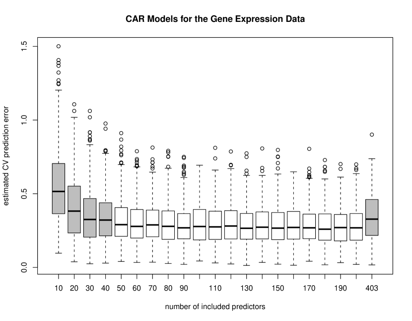
Figure 3: Comparison of CV prediction errors of CAR regression models of various sizes for the gene expression data.

On this $30\times 403$ data matrix we fitted regression models using shrinkage CAR, lasso, and elastic net. The optimal tuning parameters were selected by minimizing prediction error estimated by 5-fold cross-validation with 100 repeats. Cross-validation included model selection as integrative step, e.g., CAR scores were recomputed in each repetition in order to avoid downward bias. A summary of the results is found in Tab. 9. The prediction error of the elastic net regression model is substantially smaller than that of the lasso model, at the cost of 49 additionally included covariates. The regression model suggested by the CAR approach for the same model sizes improves over both models. As can be seen from Fig. 3 the optimal CAR regression model has a size of about 60 predictors. The inclusion of additional explanatory variables does not substantially improve prediction accuracy.

6 Conclusion

We have proposed correlation-adjusted marginal correlations $\boldsymbol{\omega}$, or CAR scores, as a means of assigning variable importance to individual predictors and to perform variable selection. This approach is based on simultaneous orthogonalization of the covariables by Mahalanobis-decorrelation and subsequently estimating the remaining correlation between the response and the sphered predictors.

We have shown that CAR scores not only simplify the regression equations but more importantly result in a canonical ordering of variables that provides the basis for a simple yet highly effective procedure for variable selection. Because of the orthogonal compatibility of squared CAR scores they can also be used to assign variable importance to groups of predictors. In simulations and by analyzing experimental data we have shown that CAR score regression is competitive in terms of prediction and model error with regression approaches such as elastic net, lasso or boosting.

Since writing of this paper in 2010 we have now also become aware of the “tilted correlation” approach to variable selection (Cho and Fryzlewicz,, 2011). The tilted correlation — though not identical to the CAR score — has the same objective, namely to provide a measure of the contribution of each covariable in predicting the response while taking account of the correlation among explanatory variables.

In summary, as exemplified in our analysis we suggest the following strategy for analyzing high-dimensional data, using CAR scores for continuous and CAT scores for categorical response:

1. Prescreen predictor variables using marginal correlations (or $t$-scores) with an adaptive threshold determined, e.g., by controlling FNDR (Ahdesmäki and Strimmer,, 2010).

2. Rank the remaining variables by their squared CAR (or CAT) scores.

3. If desired, group variables and compute grouped CAR (or CAT) scores.

Currently, we are studying algorithmic improvements to enable shrinkage estimation of CAT and CAR scores even for very large numbers of predictors and correlation matrices, which may render unnecessary in many cases the prescreening step above.

References

- Ackermann and Strimmer, (2009) Ackermann, M. and Strimmer, K. (2009). A general modular framework for gene set enrichment. BMC Bioinformatics, 10:47.
- Ahdesmäki and Strimmer, (2010) Ahdesmäki, M. and Strimmer, K. (2010). Feature selection in omics prediction problems using cat scores and false non-discovery rate control. Ann. Appl. Statist., 4:503–519.
- Akaike, (1974) Akaike, H. (1974). A new look at the statistical model identification. IEEE Trans. Automat. Control, 19:716–723.
- Bondell and Reich, (2008) Bondell, H. D. and Reich, B. J. (2008). Simultaneous regression shrinkage, variable selection, and supervised clustering of predictors with OSCAR. Biometrics, 64:115–123.
- Bring, (1994) Bring, J. (1994). How to standardize regression coefficients. The American Statistician, 48:209–213.
- Cho and Fryzlewicz, (2011) Cho, H. and Fryzlewicz, P. (2011). High-dimensional variable selection via tilting. Preprint.
- Efron et al., (2004) Efron, B., Hastie, T., Johnstone, I., and Tibshirani, R. (2004). Least angle regression (with discussion). Ann. Statist., 32:407–499.
- Fan and Lv, (2008) Fan, J. and Lv, J. (2008). Sure independence screening for ultra-high dimensional feature space (with discussion). J. R. Statist. Soc. B, 70:849–911.
- Fan and Lv, (2010) Fan, J. and Lv, J. (2010). A selective overview of variable selection in high dimensional feature space. Statistica Sinica, 20:101–148.
- Firth, (1998) Firth, D. (1998). Relative importance of explanatory variables. In Conference on Statistical Issues in Social Sciences, Stockholm, October 1998.
- Foster and George, (1994) Foster, D. P. and George, E. I. (1994). The risk inflation criterion for multiple regression. Ann. Statist., 22:1947–1975.
- Genizi, (1993) Genizi, A. (1993). Decomposition of in multiple regression with correlated regressors. Statistica Sinica, 3:407–420.
- George, (2000) George, E. I. (2000). The variable selection problem. J. Amer. Statist. Assoc., 95:1304–1308.
- Grömping, (2007) Grömping, U. (2007). Estimators of relative importance in linear regression based on variance decomposition. The American Statistician, 61:139–147.
- Hastie et al., (2009) Hastie, T., Tibshirani, R., and Friedman, J. (2009). The Elements of Statistical Learning: Data Mining, Inference, and Prediction. Springer, 2nd edition.
- Hoffman, (1960) Hoffman, P. J. (1960). The paramorphic representation of clinical judgment. Psychol. Bull., 57:1116–131.
- Hothorn and Bühlmann, (2006) Hothorn, T. and Bühlmann, P. (2006). Model-based boosting in high dimensions. Bioinformatics, 22:2828–2829.
- Hyvärinen et al., (2001) Hyvärinen, A., Karhunen, J., and Oja, E. (2001). Independent Component Analysis. John Wiley & Sons.
- Li and Li, (2008) Li, C. and Li, H. (2008). Network-constrained regularization and variable selection for analysis of genomic data. Bioinformatics, 24:1175–1182.
- Li and Lin, (2010) Li, Q. and Lin, N. (2010). The Bayesian elastic net. Bayesian Analysis, 5:151–170.
- Lu et al., (2004) Lu, T., Pan, Y., Kao, S.-Y., Li, C., Kohane, I., Chan, J., and Yankner, B. A. (2004). Gene regulation and DNA damage in the ageing human brain. Nature, 429:883–891.
- Mallows, (1973) Mallows, C. L. (1973). Some comments on . Technometrics, 15:661–675.
- Opgen-Rhein and Strimmer, (2007) Opgen-Rhein, R. and Strimmer, K. (2007). From correlation to causation networks: a simple approximate learning algorithm and its application to high-dimensional plant gene expression data. BMC Systems Biology, 1:37.
- Pratt, (1987) Pratt, J. W. (1987). Dividing the indivisible: using simple symmetry to partion variance explained. In Pukkila, T. and Puntanen, S., editors, Proceeding of Second Tampere Conference in Statistics, pages 245–260. University of Tampere, Finland.
- R Development Core Team, (2010) R Development Core Team (2010). R: A language and environment for statistical computing. R Foundation for Statistical Computing, Vienna, Austria. ISBN 3-900051-07-0.
- Schäfer and Strimmer, (2005) Schäfer, J. and Strimmer, K. (2005). A shrinkage approach to large-scale covariance matrix estimation and implications for functional genomics. Statist. Appl. Genet. Mol. Biol., 4:32.
- Schwarz, (1978) Schwarz, G. (1978). Estimating the dimension of a model. Ann. Statist., 6:461–464.
- Tibshirani, (1996) Tibshirani, R. (1996). Regression shrinkage and selection via the lasso. J. R. Statist. Soc. B, 58:267–288.
- Wang et al., (2011) Wang, S., Nan, B., Rosset, S., and Zhu, J. (2011). Random lasso. Ann. Applied Statistics, 5:468–485.
- Whittaker, (1990) Whittaker, J. (1990). Graphical Models in Applied Multivariate Statistics. Wiley, New York.
- Witten and Tibshirani, (2009) Witten, D. M. and Tibshirani, R. (2009). Covariance-regularized regression and classification for high-dimensional problems. J. R. Statist. Soc. B, 71:615–636.
- Zou and Hastie, (2005) Zou, H. and Hastie, T. (2005). Regularization and variable selection via the elastic net. J. R. Statist. Soc. B, 67:301–320.
- Zuber and Strimmer, (2009) Zuber, V. and Strimmer, K. (2009). Gene ranking and biomarker discovery under correlation. Bioinformatics, 25:2700–2707.