Interferometry with Two Pairs of Spin Correlated Photons

Abstract

We propose a new experiment employing two independent sources of spin correlated photon pairs. Two photons from different unpolarized sources each pass through a polarizer to a detector. Although their trajectories never mix or cross they exhibit 4th–order–interference–like correlations when the other two photons interfere on a beam splitter even when the latter two do not pass any polarizers at all. A wave packet calculation shows that the experiment permits a very discriminatory test of hidden variable theories.

Higher order interference effects have been much investigated because their nonlocal nature provides a powerful tool for testing hidden variables–theories Ou (1988); Mandel (1983); Paul (1986); Rarity et al. (1990); Ou et al. (1990, 1990); Ou and Mandel (1988); Ou et al. (1988, 1987); Campos et al. (1990); Horne et al. (1989); Wang et al. (1991); Holland and Vigier (1991); Wang et al. (1991); Silverman (1993). In a recent test Ou and Mandel Ou and Mandel (1988) used the polarization correlation of signal and idler photon of downconverted light and found a violation of Bell’s inequality by about six standard deviations. However their detectors were not sufficiently efficient. The idea was extended to two–particle interferometry in a proposal by Horne, Shimony and Zeilinger Horne et al. (1989). In another recent experiment Wang, Zou, and Mandel Wang et al. (1991) tested the so-called de Broglie–Bohm pilot wave theory. The result was negative but the set–up was recognized to lack generality by Holland and Vigier Holland and Vigier (1991) and by Wang, Zou, and Mandel Wang et al. (1991). Thus excluding realistic nonlocality remains a challenge Bell (1986).

In this paper we propose an experiment which should be the first realization of the 4th order interference of randomly prepared independent photons correlated in polarization and coming from independent sources. The experiment is based on a newly discovered interference effect of the 4th order on a beam splitter Pavičić (1994). The essential new element of the experiment is that it puts together systems which were not in any way influenced by preparation, makes them interact, and then allows us inferring overall polarization (spin) correlations — from the assumed quantum mechanical description of the unknown initial states — by simultaneous measurement of four photons separated in space. Particular polarization (spin) correlations, unexpectedly found between photons which did not in any way directly interact and on the distant pairs of which polarization has not been measured at all, are expected to be confirmed by a future experiment. Such experiments might eventually disprove any realistic hidden variable theory.

A schematic representation of the experiment is shown in Fig. 1. Two independent sources, $S_{I}$ and $S_{II}$, both simultaneously emit two photons correlated in polarization to the left and right. On the left photons we measure polarizations by the polarization filters P1 and P2 and on the right photons by P3 and P4. Because of the beam splitter the paths leading through P3 and P4 are available to the right photons from both source $S_{I}$ and source $S_{II}$. The resulting 4th order interference will manifest itself in the probability of quadruple coincidence counts in detectors D1, D2, D3 and D4.

The sources can be atoms exhibiting cascade emission. (Downconversion is not possible because it gives polarized photons.) The atoms of the two sources could be pumped to an upper level by two independent lasers Ou et al. (1987). This level would decay by emitting two photons correlated in polarization Aspect et al. (1982). The independence of the two sources can be assured by slight differences in central frequency and drift of the two pump lasers. Hence there should be no 2nd order interference at detectors D3 and D4, which could also be suppressed when the size of the sources exceeds the coherence length of the emitted photons. Interference of 4th order would still occur, because its relevant coherence time is given by the inverse of the frequency difference of the two correlated photons Ou (1988); Mandel (1983); Paul (1986); Rarity et al. (1990).

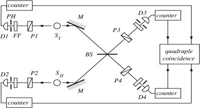
Figure 1: Lay–out of the proposed experiment.

The state of the four photons immediately after leaving the sources is described by the product of two entangled states:

$$|\Psi\rangle = {1\over\sqrt{2}}\left(|1_{x}\rangle_{1}|1_{x}\rangle_{3}\>+\>\,|1_{y}\rangle_{1}|1_{y}\rangle_{3}\right)$$ (1)

$$\otimes{1\over\sqrt{2}}\left(|1_{x}\rangle_{2}|1_{x}\rangle_{4}\>+\>\,|1_{y}\rangle_{2}|1_{y}\rangle_{4}\right)$$

Here, $|_{x}\rangle$ and $|_{y}\rangle$ denote the mutually orthogonal photon states. So, e.g., $|1_{x}\rangle_{1}$ means the state of photon 1 leaving the source $S_{I}$ to the left polarized in direction $x$. In the following we use the annihilation operator formalism, often employed in quantum optical analysis, e.g. by Paul Paul (1986), Mandel’s group Ou et al. (1990, 1990, 1987), and Campos et al. Campos et al. (1990). The operator describing the polarization at P1 oriented along the $x$-axis and the subsequent detection at D1 acts as follows: ${\hat{a}}_{1x}|1_{x}\rangle_{1}=|0_{x}\rangle_{1}$,  ${\hat{a}}_{1x}^{\dagger}|0_{x}\rangle_{1}=|1_{x}\rangle_{1}$,  ${\hat{a}}_{1x}|0_{x}\rangle_{1}=0$, etc. Paul (1986). When P1 is oriented at some angle $\theta_{1}$ polarization and detection are represented by ${\hat{a}}_{1}={\hat{a}}_{1x}\cos\theta_{1}+{\hat{a}}_{1y}\sin\theta_{1}$. The phase the photon accumulates between the source $S_{I}$ and the detector D1 adds the factor $e^{i\omega_{1}(r_{1}/c+t^{I}_{0}-t_{1})}$, where $\omega_{1}$ is the frequency of photon 1, $r_{1}$ is the path length from $S_{I}$ to D1, $c$ is the velocity of light, $t^{I}_{0}$ is the time of emission of a pair of photons at $S_{I}$, and $t_{1}$ is the time of detection at D1. Hence the annihilation of a photon at detector D1 means application of the operator ${\hat{E}}_{1}=({\hat{a}}_{1x}\cos\theta_{1}+{\hat{a}}_{1y}\sin\theta 1)e^{i\omega_{1}(r_{1}/c+t^{I}_{0}-t_{1})}$ onto the initial state of Eq. (1). Similarly, detection of photon 2 at D2 means application of ${\hat{E}}_{2}=({\hat{a}}_{2x}\cos\theta_{2}+{\hat{a}}_{2y}\sin\theta_{2})e^{i\omega_{2}(r_{2}/c+t^{II}_{0}-t_{2})}$, where the symbols are defined by analogy. On the right side of the sources, a detection at D3 can be caused by photon 3 emitted by source $S_{I}$ or by photon 4 emitted by source $S_{II}$. The beamsplitter BS may have polarization dependent transmission and reflection coefficients, denoted by $T_{x}$, $T_{y}$, and $R_{x}$, $R_{y}$, respectively. The angle of the polarizer P3 is given by $\theta_{3}$. Hence we obtain

$$\hat{E}_{3}=\!\!\left(\hat{a}_{4x}\sqrt{T_{x}}\cos\theta_{3}+\hat{a}_{4y}\sqrt{T_{y}}\sin\theta_{3}\right)\!e^{i\,\omega_{4}({r_{{}_{II}}\!+r_{3}\over c}+t_{{}_{0}}^{{}^{II}}\!-t_{3})}$$

$$+i\left(\hat{a}_{3x}\sqrt{R_{x}}\cos\theta_{3}+\hat{a}_{3y}\sqrt{R_{y}}\sin\theta_{3}\right)e^{i\,\omega_{3}({r_{{}_{I}}+r_{3}\over c}+t_{{}_{0}}^{{}^{I}}-t_{3})}$$

With similar arguments the interactions leading to registration of a photon at detector D4 are given by the operator

$$\hat{E}_{4}=\left(\hat{a}_{3x}\sqrt{T_{x}}\cos\theta_{4}+\hat{a}_{3y}\sqrt{T_{y}}\sin\theta_{4}\right)e^{i\,\omega_{3}({r_{{}_{I}}+r_{4}\over c}+t_{{}_{0}}^{{}^{I}}-t_{4})}$$

$$+i\left(\hat{a}_{4x}\sqrt{R_{x}}\cos\theta_{4}+\hat{a}_{4y}\sqrt{R_{y}}\sin\theta_{4}\right)e^{i\,\omega_{4}({r_{{}_{II}}+r_{4}\over c}+t_{{}_{0}}^{{}^{II}}-t_{4})}$$

Here, $r_{I}$ and $r_{II}$ denote the distance from the respective source to the beamsplitter, $r_{3}$ denotes the distance from the beamsplitter to detector D3, $t_{3}$ is the time of detection at D3, and $\omega_{3}$ is the frequency of photon 3. The symbols $r_{4}$, $t_{4}$ and $\omega_{4}$ are defined analogously. The evolution of the initial state through interaction with the whole setup including detection of one photon in each detector is then given by:

$$\hat{E}_{4}\hat{E}_{3}\hat{E}_{2}\hat{E}_{1}|\Psi\rangle= e^{i\,[\omega_{1}({r_{{}_{1}}\over c}+t_{{}_{0}}^{{}^{I}}-t_{1})+\omega_{2}({r_{{}_{2}}\over c}+t_{{}_{0}}^{{}^{II}}-t_{2})+\omega_{3}({r_{{}_{I}}\over c}+t_{{}_{0}}^{{}^{I}})+\omega_{4}({r_{{}_{II}}\over c}+t_{{}_{0}}^{{}^{II}})]}$$ (2)

$$\times \bigl{\{}T_{14}T_{23}\,e^{i\,[\omega_{3}({r_{{}_{4}}\over c}-t_{{}_{4}})+\omega_{4}({r_{{}_{3}}\over c}-t_{{}_{3}})]}-R_{24}R_{13}\,e^{i\,[\omega_{3}({r_{{}_{3}}\over c}-t_{{}_{3}})+\omega_{4}({r_{{}_{4}}\over c}-t_{{}_{4}})]}\bigr{\}}|0\rangle$$

where

$$T_{ij}=\sqrt{T_{x}}\cos\theta_{i}\cos\theta_{j}+\sqrt{T_{y}}\sin\theta_{i}\sin\theta_{j},$$

$$R_{ij}=\sqrt{R_{x}}\cos\theta_{i}\cos\theta_{j}+\sqrt{R_{y}}\sin\theta_{i}\sin\theta_{j}.$$ (3)

The squared modulus of this result gives the probability of having one photon arrive in each detector as a function of the angles of the polarizers. Note that the interference term, which is the real part of the product of the two terms in brackets, contains only the detection times $t_{3}$ and $t_{4}$ at detectors D3 and D4, respectively. Hence we would expect the 4th order interference to occur only in the coincidence counts of those two detectors. However, assuming for simplicity $r_{I}=r_{II}$, $r_{3}=r_{4}$, $\omega_{3}=\omega_{4}$, and $T_{x}=T_{y}=R_{x}=R_{y}=1/2$, we get for the coincidence probability:

$$P(\theta_{1},\theta_{2},\theta_{3},\theta_{4})= \langle\Psi|{\hat{E}}_{1}^{\dagger}{\hat{E}}_{2}^{\dagger}{\hat{E}}_{3}^{\dagger}{\hat{E}}_{4}^{\dagger}{\hat{E}}_{4}{\hat{E}}_{3}{\hat{E}}_{2}{\hat{E}}_{1}|\Psi\rangle$$

$$= {\textstyle{1\over 16}}\sin^{2}(\theta_{1}-\theta_{2})\sin^{2}(\theta_{3}-\theta_{4})$$ (4)

The correlations thus exist between the polarizations on the right side and between those on the left side. This means that the two photons going to the left can be forced into a nonlocal polarization correlation although they are emitted from two independent sources and nowhere share a common trajectory. Moreover, the correlation does not depend on the frequencies of the two photons, nor is there any condition as to the permissible time interval $|t_{1}-t_{2}|$ between their detections. This can be seen in Eq. (2) where the relevant parameters $(\omega_{1},\omega_{2},t_{1},t_{2},r_{1},r_{2})$ only enter in the overall phase factor in contrast to photons 3 and 4, which must be detected within a time interval shorter than the beating period $|\omega_{3}-\omega_{4}|^{-1}$.

It is now interesting to see that the nonlocal polarization correlation between the photons on one side persists even when the polarizers on the other side are removed. Without the polarizers P1 and P2 of the left side, we have to sum over the probabilities of the four possible orthogonal settings of these polarizers and obtain

$$P(\infty,\infty,\theta_{3},\theta_{4}) = {1\over 8}\Bigl{\{}1-\cos^{2}(\theta_{3}-\theta_{4})\cos\bigl{[}(\omega_{3}-\omega_{4})$$ (5)

$$\times \bigl{(}{r_{4}-r_{3}\over c}+t_{3}-t_{4}\bigr{)}\bigr{]}\Bigr{\}}$$

where we set $r_{I}=r_{II}$ and $T_{x}=T_{y}=R_{x}=R_{y}=1/2$, but otherwise put no restrictions on the frequencies of the photons, the path lengths to the detectors, or the detection times. Eq. (5) expresses the kind of nonlocal correlations from independent sources proposed by Yurke and Stoler Yurke and Stoler (1992).

On the other hand, if we remove the polarizers of the right side, P3 and P4, we find

$$P(\theta_{1},\theta_{2},\infty,\infty) = {1\over 8}\Bigl{\{}1-\cos^{2}(\theta_{1}-\theta_{2})\cos\bigl{[}(\omega_{3}-\omega_{4})$$ (6)

$$\times \bigl{(}{r_{4}-r_{3}\over c}+t_{3}-t_{4}\bigr{)}\bigr{]}\Bigr{\}}$$

We see here explicitly, that the two photons on the left side can show a nonlocal correlation only if the time interval between detections on the right side, $|t_{3}-t_{4}|$, is kept below the beating frequency of the photons on the right side. This condition becomes trivial when we have $\omega_{3}=\omega_{4}$. Then the above expression suggests that there should be a time independent nonlocal polarization correlation between photons 1 and 2, although no polarization is measured on photons 3 and 4. At first glance this appears to be equivalent to having two independent 1-particle sources emitting unpolarized photons of different frequencies, which nowhere meet before their detection, and which yet are supposed to show nonlocal polarization correlations that are constant in time and we would expect no polarization correlation in such a situation. But also the result of Eq. (5) is surprising, because it is what Ou and Mandel obtained Ou and Mandel (1988); Ou et al. (1988) for the interference of the two orthogonally polarized signal and idler beams of downconverted light, while we are dealing with originally unpolarized beams.

In order to see whether the nonlocal correlations of eqs. (4) and (5) can be used to test Bell’s inequality we turn to a more realistic description by means of wave packets. Each photon is represented by a gaussian amplitude distribution of energies. For the sake of simplicity all four photons shall have the same width of the energy distribution and thus the same coherence time T. The probability amplitude that photon $i$ has frequency $\omega_{i}$ when its central frequency is $\omega_{i0}$ is given by

$$f(\omega_{i},\omega_{i0},T)={\textstyle{{T^{1/2}\over\pi^{1/4}}}}e^{-(\omega_{i}-\omega_{i0})^{2}T^{2}/2}\ \ \ \ \ \ \ \ \ \ {\rm with}\ i=1,\dots,4$$

where we normalized $|f_{i}|^{2}$ to 1. The final state of Eq. (2) must be multiplied with these four functions and integrations must be made over the frequencies $\omega_{i},i=1,...,4$. This models a photon pair as two wave packets fully overlapping at the source at the time of emission and then moving apart. Now Eqs. (4) and (5) turn into

$$P(\infty,\infty,\theta_{3},\theta_{4}) = {F\over T^{4}}\Bigl{\{}\cosh(\tau_{s}\tau_{34}/T^{2})$$ (7)

$$- \cos^{2}(\theta_{3}-\theta_{4})\cos\bigl{[}(\omega_{3}-\omega_{4})\tau_{34}\bigr{]}\Bigr{\}}\qquad$$

$$P(\theta_{1},\theta_{2},\infty,\infty) = {F\over T^{4}}\Bigl{\{}\cosh(\tau_{s}\tau_{34}/T^{2})$$ (8)

$$- \cos^{2}(\theta_{1}-\theta_{2})\cos\bigl{[}(\omega_{3}-\omega_{4})\tau_{34}\bigr{]}\Bigr{\}}\qquad$$

where we set $r_{3}=r_{4}$ and defined $\tau_{s}\equiv t_{0}^{I}-t_{0}^{II}$ and $\tau_{34}\equiv t_{3}-t_{4}$. We are now dealing with probability densities for a quadruple detection at time points $t_{1}$, $t_{2}$, $t_{3}$ and $t_{4}$. The damping term $F$ contains the detection times $t_{1}$ and $t_{2}$ and other experimental parameters. It expresses how well the wavepackets are centered at the various detectors at the respective detection times. Note that in both cases the polarization correlations persist but are reduced in visibility, which is given by $v=\bigl{[}2\cosh(\tau_{s}\tau_{34}/T^{2})-1\bigr{]}^{-1}$ when $(\omega_{30}-\omega_{40})\tau_{34}=0$. For a violation of Bell’s inequality, and hence for a possible exclusion of hidden variable theories, $v$ must be larger than $2^{-1/2}$ implying the product $\tau_{34}\tau_{s}$ must be less than $0.663T^{2}$. However, the time interval between the emissions at the two sources, $\tau_{s}$, is not a directly measurable quantity, but must be inferred from the detection times. Therefore $\tau_{s}$ cannot be known better than to about $T$. Hence $\tau_{34}<<T$ is a necessary requirement, which means D3 and D4 must fire in ultra short coincidence. In consequence most of the data collected at D3 and D4 must be discarded, as even for simultaneous emissions from the sources the mean value of $\tau_{34}$ is about $\sqrt{2}T$. This in turn precludes a test of local hidden variable theories by means of Bell’s inequality at detectors D3 and D4, where a postselection throws away more than 31% of the data Garg and Mermin (1987). On the other hand, the test is possible at detectors D1 and D2 [Eq. (8)]. Again the requirement is for ultra short coincidence at detectors D3 and D4 and not at D1 and D2, where there is no upper bound on the coincidence window $|t_{1}-t_{2}|$. In fact one would permit a wide coincidence window in order to collect all data at D1 and D2 that have been preselected by the ultra short coincidence between D3 and D4. This constitutes a most discriminating test of Bell’s inequality, because no postselection of the nonlocally correlated particles 1 and 2 is needed.

Let us now conclude with an attempt to understand how the polarization correlation of the particles on the left side can come about even when there are no polarizers on the right side and why only the mutual angles on each side — Eq. (4) — are relevant for the overall coincidences. The answer lies in the beam splitter. It superimposes the states of photon 3 and 4. The beams going to detectors D3 and D4 must therefore reflect the bosonic character of the particles and can only be occupied in the following two ways:

(a) Both photons in the same beam. The commutation rules demand that the two photons, e.g., from the beam going to D3 (assuming $r_{I}=r_{II}$, $r_{3}=r_{4}$, and $T_{x}=T_{y}=R_{x}=R_{y}=1/2$) obey the following counterpart of Eq. (4):

$$P(\theta_{1},\theta_{2},2\times\theta_{3})= \langle\Psi|{\hat{E}}_{1}^{\dagger}{\hat{E}}_{2}^{\dagger}{\hat{E}}_{3}^{\dagger}{\hat{E}}_{3}^{\dagger}{\hat{E}}_{3}{\hat{E}}_{3}{\hat{E}}_{2}{\hat{E}}_{1}|\Psi\rangle$$

$$={\textstyle{1\over 4}}\cos^{2}(\theta_{1} -\theta_{3})\cos^{2}(\theta_{2}-\theta_{3})$$ (9)

given they have the same energy ($\omega_{3}=\omega_{4}$). When there are no polarizers before D3 and D4, photons 1 and 2 going to the left would still have the polarization correlation, but individually they would be unpolarized. For both 2–photons channels together we obtain $P(\theta_{1},\theta_{2},\infty,\infty)=[1+\cos^{2}(\theta_{1}-\theta_{2})]/8$.

(b)One photon in each beam: 1-1–channel. Now the commutation rules require that the polarizations are correlated as given by Eq. (4). This means we also get the correlation between the polarizations of beams 1 and 2 as given by Eq. (6): $P(\theta_{1},\theta_{2},\infty,\infty)=\sin^{2}(\theta_{1}-\theta_{2})/8$, i.e., with the maximum in the orthogonal direction with regard to the previous case.

Of course, the polarization correlation between photons 1 and 2 disappears if we do not detect them in coincidence detections on the right side, which one can see from the fact that the sum of $P(\theta_{1},\theta_{2},\infty,\infty)$ from all the channels is a constant.

To understand Eq. (4) let us compare it with the standard left–right Bell probabilities: $P(\theta_{1},\theta_{3})={1\over 2}cos^{2}(\theta_{1}-\theta_{3})$ and $P(\theta_{2},\theta_{4})={1\over 2}cos^{2}(\theta_{2}-\theta_{4})$. For the angles $\theta_{1}=\theta_{2}$ and $\theta_{3}=\theta_{4}$ we obtain [from Eq. (4)] $P(\theta_{1},\theta_{3},\theta_{2},\theta_{4})=0$ no matter the values of $\theta_{1}-\theta_{3}$ and $\theta_{2}-\theta_{4}$. These three probabilities clearly cannot be satisfied simultaneously and we can express this fact by saying that the 4th order interference erases information on polarization correlation in the 1-1–channel. An immediate consequence is that for $\theta_{1}=\theta_{2}=\theta_{3}=\theta_{4}$ we can never register coincidences and this represents yet another possibility to formulate Bell’s theorem without inequalites — the idea first developed by Greenberger, Horne, and Zeilinger Greenberger et al. (1989). The possiblity is based on the well–known fact that the classical visibility of the 4th order interference is not higher than 50%.

It is interesting that although for $\omega_{3}\neq\omega_{4}$ we can track down the Bell left–right probabilities in the 2–photons beams exactly, as expected, in the 1-1–channel this is even then not possible. The case of different energies can be handled with frequency filters (FF in Fig. 1). The result is then modulated with the beating period but in effect we have $P(\theta_{1},\theta_{2},\theta_{3},\theta_{4})={\textstyle{1\over 2}}\cos^{2}(\theta_{1}-\theta_{3})\cos^{2}(\theta_{2}-\theta_{4})$ if we assume two polarizers and two detectors in each 2–photons beam (not shown in Fig. 1). So, dropped polarizer in front of the one of the four detectors immediately gives the standard left–right Bell probability for the other pair. The 1-1–channel, on the other hand, responds to the special feature of the interference of the 4th order to “create” the polarization correlation even when unpolarized photons interfere — see Eq. (5).

Thus, while the 2nd order interference erases the path memory, the 4th order interference erases the polarization correlation memory. It occurs in an analogous way in which the 4th order interference erases the polarization memory of two polarized incident photons according to Eq. (16) of Ref. Pavičić (1994).

One of us (M.P.) is grateful to his host K.-E. Hellwig, Inst. Theor. Physics, TU Berlin where he completed the first draft of the present paper containing the full elaboration in the plane waves and discussed it in a series of 4 seminars he held at TU Berlin (Jul 16 - Aug 9, 1993).

References

- Ou (1988) Z. Y. Ou, Phys. Rev. A, 37, 1607 (1988).
- Mandel (1983) L. Mandel, Phys. Rev. A, 28, 929 (1983).
- Paul (1986) H. Paul, Rev. Mod. Phys., 58, 209 (1986).
- Rarity et al. (1990) J. G. Rarity, P. R. Tapster, E. J. T. Larchuk, R. A. Campos, M. C. Teich, and B. E. A. Saleh, Phys. Rev. Lett., 65, 1348– (1990).
- Ou et al. (1990) Z. Y. Ou, X. Y. Zou, L. J. Wang, and L. Mandel, Phys. Rev. A, 42, 2957 (1990a).
- Ou et al. (1990) Z. Y. Ou, L. J. Wang, X. Y. Zou, and L. Mandel, Phys. Rev. A, 41, 566 (1990b).
- Ou and Mandel (1988) Z. Y. Ou and L. Mandel, Phys. Rev. Lett., 61, 50 (1988).
- Ou et al. (1988) Z. Y. Ou, C. Hong, and L. Mandel, Opt. Commun., 67, 169 (1988).
- Ou et al. (1987) Z. Y. Ou, C. Hong, and L. Mandel, Phys. Lett. A, 122, 11 (1987).
- Campos et al. (1990) R. A. Campos, B. E. A. Saleh, and M. C. Teich, Phys. Rev. A, 42, 4127– (1990).
- Horne et al. (1989) M. A. Horne, A. Shimony, and A. Zeilinger, Phys. Rev. Lett, 62, 2209– (1989).
- Wang et al. (1991) L. J. Wang, X. Y. Zou, and L. Mandel, Phys. Rev. Lett., 66, 1111 (1991a).
- Holland and Vigier (1991) P. R. Holland and J. P. Vigier, Phys. Rev. Lett., 67, 402 (1991).
- Wang et al. (1991) L. J. Wang, X. Y. Zou, and L. Mandel, Phys. Rev. Lett., 67, 403 (1991b).
- Silverman (1993) M. P. Silverman, Am. J. Phys., 61, 514 (1993).
- Bell (1986) J. S. Bell, Phys. Reports, 137, 7 (1986).
- Pavičić (1994) M. Pavičić, Phys. Rev. A, 50, 3486 (1994).
- Aspect et al. (1982) A. Aspect, J. Dalibard, and G. Roger, Phys. Rev. Lett., 49, 1804 (1982).
- Note (1) For the given operators cf. Refs. Ou (1988); Ou et al. (1990); Ou and Mandel (1988); Ou et al. (1988) Note that positive imaginary terms assure the preservation of boson commutation relations for the anihilation operators at the output of the beam splitter and that Eqs. (2), (5a), etc. of Ref. Ou and Mandel (1988) and Eqs. (56), (57), etc. of Ref. Ou (1988) should be corrected accordingly. Harry Paul also noticed the latter fact (private communication).
- Yurke and Stoler (1992) B. Yurke and D. Stoler, Phys. Rev. Lett., 68, 1251– (1992).
- Garg and Mermin (1987) A. Garg and N. D. Mermin, Phys. Rev. D, 35, 3831– (1987).
- Greenberger et al. (1989) D. M. Greenberger, M. Horne, and A. Zeilinger, in Bell’s Theorem, Quantum Theory, and Conceptions of the Universe, edited by N. Kafatos (Kluwer, Dordrect, 1989) pp. 69–72.