Scattering of rough solutions of the nonlinear Klein-Gordon equations in 3D

Abstract.

We prove scattering of solutions below the energy norm of the nonlinear Klein-Gordon equation in 3D with a defocusing power-type nonlinearity that is superconformal and energy subcritical: this result extends those obtained in the energy class [4, 18, 19] and those obtained below the energy norm under the additional assumption of spherical symmetry [25]. In order to do that, we generate an exponential-type decay estimate in $H^{s}$, $s<1$, by means of concentration [1] and a low-high frequency decomposition [2, 7] : this is the starting point to prove scattering. On low frequencies we modify the arguments in [18, 19]; on high frequencies we use the smoothing effect of the solutions to control the error terms: this, combined with an almost conservation law, allows to prove this decay estimate.

1. Introduction and Theorem

In this paper we consider the defocusing nonlinear Klein-Gordon equation on $\mathbb{R}^{3}$:

(1.1) $$\partial_{tt}u-\Delta u+u=-|u|^{p-1}u$$

with data $u(0)=u_{0}$, $\partial_{t}u(0)=u_{1}$ lying in $H^{s}$, $H^{s-1}$ respectively.
We are interested in the strong solutions of the defocusing nonlinear Klein-Gordon equation on some interval $[0,T]$ i.e maps $u$, $\partial_{t}u$ that lie in $C\left([0,\,T],\,H^{s}(\mathbb{R}^{3})\right)$, $C\left([0,\,T],\,H^{s-1}(\mathbb{R}^{3})\right)$ respectively and that satisfy

(1.2) $$u(t)=\cos{(t\langle D\rangle)}u_{0}+\frac{\sin(t\langle D\rangle)}{\langle D\rangle}u_{1}-\int_{0}^{t}\frac{\sin\left((t-t^{{}^{\prime}})\langle D\rangle\right)}{\langle D\rangle}|u|^{p-1}(t^{{}^{\prime}})u(t^{{}^{\prime}})\,dt^{{}^{\prime}}.$$

The defocusing nonlinear Klein-Gordon equation is closely related to the defocusing nonlinear wave equation:

(1.3) $$\partial_{tt}v-\triangle v=-|v|^{p-1}v$$

with data $v(0):=v_{0}$, $\partial_{t}v(0):=v_{1}$. (1.3) enjoys the following scaling property

(1.4) $$v(t,x)\rightarrow\frac{1}{\lambda^{\frac{2}{p-1}}}v\left(\frac{t}{\lambda},\frac{x}{\lambda}\right),\quad v_{0}(x)\rightarrow\frac{1}{\lambda^{\frac{2}{p-1}}}v_{0}\left(\frac{x}{\lambda}\right),\quad v_{1}(x)\rightarrow\frac{1}{\lambda^{\frac{2}{p-1}+1}}v_{1}\left(\frac{x}{\lambda}\right).$$

We define the critical exponent $s_{c}:=\frac{3}{2}-\frac{2}{p-1}$. One can check that the $\dot{H}^{s_{c}}\times\dot{H}^{s_{c}-1}$ norm of $(u_{0},u_{1})$ is invariant under the scaling transformation (1.4) . (1.1) is known to be locally well-posed in $H^{s}\times H^{s-1}$, $s\geq s_{c}$, $p\geq\frac{7}{3}$ by using an iterative argument. If $p=5$ then $s_{c}=1$ and we say that the nonlinearity $|u|^{p-1}u$ is $\dot{H}^{1}$ (or energy) critical. If $p=\frac{7}{3}$ then $s_{c}=0$ and the we say that the nonlinearity is $L^{2}$ (or mass) critical. If $p=3$ then $s_{c}=\frac{1}{2}$ and we say that the nonlinearity is conformal. If $\frac{7}{3}<p<5$ then we say that the regime is mass supercritical-energy subcritical. If $3<p<5$ then we say that the regime is superconformal and energy subcritical.
It is well-known that smooth solutions of (1.1) have a conserved energy

$$E(u(t)):= \frac{1}{2}\int_{\mathbb{R}^{3}}\left|\partial_{t}u(t,x)\right|^{2}\,dx+\frac{1}{2}\int_{\mathbb{R}^{3}}|\nabla u(t,x)|^{2}\,dx+\frac{1}{2}\int_{\mathbb{R}^{3}}|u(t,x)|^{2}\,dx$$

(1.5) $$+\frac{1}{p+1}\int_{\mathbb{R}^{3}}|u(t,x)|^{p+1}\,dx.$$

In fact by standard limit arguments the energy conservation law remains true for solutions $(u,\partial_{t}u)\in H^{s}\times H^{s-1}$, $s\geq 1$. Since the lifespan of the local solution depends only on the $H^{s}\times H^{s-1}$ norm of the initial data $(u_{0},u_{1})$ (see [13]) for $s>s_{c}$, then it suffices to find an a priori pointwise in time bound in $H^{s}\times H^{s-1}$ of the solution $(u,\partial_{t}u)$ in order to establish global well-posedness.
The long-time behavior in the energy space (i.e with data $(u_{0},u_{1})\in H^{1}\times L^{2}$ ) has attracted much attention from the community. The energy captures the evolution in time of the $H^{1}\times L^{2}$ norm of the solutions. Since it is conserved we have global existence of solutions of (1.1) in the energy space for all dimension $n$ and for all exponent $p$ that is mass-supercritical and energy-subcritical, i.e $1+\frac{4}{n}<p<1+\frac{4}{n-2}$. The next stage is to understand the asymptotic behavior of the solutions of (1.1) in the energy space. The scattering, i.e the linear asymptotic behavior, was proved in [3, 4, 9, 18, 19, 20, 21] for all dimension $n$.
The long-time behavior below energy norm (i.e with data in $H^{s}\times H^{s-1}$, $s<1$) has also received much attention from the community. The global existence of solutions of (1.1) has been investigated in [24]. The scattering of solutions of (1.1) with radial data and in dimension $3$ has been studied in [25]. More precisely it was proved that the asymptotic behavior for spherical solutions is linear for $3<p<5$ and in $H^{s}\times H^{s-1}$, $\bar{\bar{s}}:=\bar{\bar{s}}(p)<s<1$ where

$$\bar{\bar{s}}:=\begin{cases}1-\frac{(5-p)(p-3)}{2(p-1)(p-2)},\,4\geq p>3\\ 1-\frac{(5-p)^{2}}{2(p-1)(6-p)},\,5>p\geq 4.\end{cases}$$

In this paper we are interested in proving scattering results for general data below the energy norm and in dimension $3$. The main result of this paper is the following one:

Theorem 1.1.

Let $5>p>3$, $A\gtrsim 1$ and $(u_{0},u_{1})\in H^{s}\times H^{s-1}$ such that

(1.6) $$\|(u_{0},u_{1})\|_{H^{s}\times H^{s-1}}\leq A.$$

Then there exists $\tilde{s}:=\tilde{s}(A,p)<1$ such that $\tilde{s}\rightarrow 1$ as $A\rightarrow\infty$ and such that the solution of (1.1) with data $(u_{0},u_{1})$ exists for all time $T$ and scatters as $T$ goes to infinity, i.e there exists $\left(u_{+,0},u_{+,1}\right)\in H^{s}\times H^{s-1}$ such that

$$\lim\limits_{T\rightarrow\infty}\|\left(u(T),\partial_{t}u(T)\right)-K(T)(u_{+,0},u_{-,0})\|_{H^{s}\times H^{s-1}}=0.$$

Here,

$$K(T):=\left(\begin{array}[]{ll}\cos{(T\langle D\rangle)}&\frac{\sin{(T\langle D\rangle)}}{\langle D\rangle}\\ -\langle D\rangle\,\sin{(T\langle D\rangle)}&\cos{(T\langle D\rangle)}\end{array}\right).$$

Remark 1.2.

In fact, as $A\rightarrow\infty$, then there exists a constant $\tilde{\alpha}:=\tilde{\alpha}(p)>1$ such that one can choose $\tilde{s}$ depending on $A$ in the following fashion:

(1.7) $$\tilde{s}=1-\frac{1}{\tilde{\alpha}^{\tilde{\alpha}^{....^{\tilde{\alpha}}}}}.$$

Here the height of the tower is $\sim A^{\tilde{\alpha}}$.

2. Notation

2.1. General notation

We set some general notation that appear throughout the proof.

If $x\in\mathbb{R}$, then $\langle x\rangle:=(1+|x|^{2})^{\frac{1}{2}}$, $x^{+}$ is a slightly larger number than $x$, $x^{++}$ is a slightly larger number than $x^{+}$, $x^{-}$ is a slightly smaller number than $x$, and $x^{--}$ is a slightly smaller number than $x^{-}$.

Let $f$ be a function differentiable in time and smooth in space. We write $F(f)$ for the following function

$$F(f):=|f|^{p-1}f.$$

Given $J$ a time interval, we denote by $X^{J}_{f}$ the following number

$$X^{J}_{f}(t):=-\int_{J}\frac{\sin{((t-s)\langle D\rangle)}}{\langle D\rangle}(f(s))\,ds$$

We denote by $W$ the set of wave admissible points, i.e

$$W:=\left\{(q,r),\,(q,r)\in(2,\infty]\times[2,\infty),\,\frac{1}{q}+\frac{1}{r}\leq\frac{1}{2}\right\}.$$

Given $m\in[0,1]$, we say that $(q,r)$ is $m-$wave admissible if

$$(q,r)\in W\quad\text{and}\quad\frac{1}{q}+\frac{3}{r}=\frac{3}{2}-m$$

and $q\geq 2+$ if $m=1$.We denote by $W_{m}$ the set of $m$-wave admissible points. We denote by $\tilde{W}$ the dual set of $W$, i.e

$$\tilde{W}:=\left\{(\tilde{x},\tilde{y}),\,\exists(x,y)\in W,\,\frac{1}{x}+\frac{1}{\tilde{x}}=1,\,\frac{1}{y}+\frac{1}{\tilde{y}}=1\right\}.$$

A graphical representation of these sets is given on Figure 1.

2.2. The multiplier $I$, the numbers $Z$, and the mollified energies $E(If)$

We introduce the multiplier $I$.

The proof of Theorem 1.1 involves the multiplier $I$ defined as follows:

$$\widehat{If}(t,\xi):=m(\xi)\hat{f}(t,\xi),$$

where

• $m(\xi):=\eta\left(\frac{\xi}{N}\right)$

• $\eta$ is a smooth, radial, nonincreasing function in $|\xi|$ such that $\eta(\xi):=1$, $|\xi|\leq 1$ and $\eta(\xi):=\frac{1}{|\xi|^{1-s}}$, $|\xi|\geq 2$

• $N\gg 1$ is a parameter.

Throughout the paper we choose $(N,s)$ such that

(2.1) $$N^{1-s}\sim 1.$$

We shall explain in Section 4 why this choice of $(N,s)$ is natural.

We introduce some numbers that we constantly use in the proof. Given $J$ a time interval, let

$$Z_{m,s}(J,f):=\sup_{\begin{subarray}{c}(q,r)-m\\ wave\,adm\end{subarray}}\|\partial_{t}\langle D\rangle^{-m}If\|_{L_{t}^{q}L_{x}^{r}(J)}+\|\langle D\rangle^{1-m}If\|_{L_{t}^{q}L_{x}^{r}(J)},$$

$$Z(J,f):=\sup_{m\in[0,1]}Z_{m,s}(J,f),$$

and

$$\begin{array}[]{ll}\tilde{Z}(J,f)&:=\|\partial_{t}\langle D\rangle^{-\frac{1}{2}}If\|_{L_{t}^{4}L_{x}^{4}(J)}+\|\langle D\rangle^{1-\frac{1}{2}}If\|_{L_{t}^{2(p-1)-}L_{x}^{\frac{6(p-1)}{2p-3}+}(J)}+\|If\|_{L_{t}^{2(p-1)-}L_{x}^{2(p-1)+}(J)}\\ &+\|\langle D\rangle^{1-\frac{2}{p}}If\|_{L_{t}^{p}L_{x}^{\frac{2p}{p-2}}(J)}+\|\langle D\rangle^{1-\frac{3p-5}{2p}}If\|_{L_{t}^{p}L_{x}^{2p}(J)}+\|\langle D\rangle^{1-\frac{1}{2}}If\|_{L_{t}^{4+}L_{x}^{4-}(J)}\\ &+\|\langle D\rangle^{1-\frac{p-3}{2}}If\|_{L_{t}^{\frac{4}{p-3}}L_{x}^{\frac{4}{5-p}}(J)}+\|\langle D\rangle^{1-1}If\|_{L_{t}^{\frac{4(p-1)}{7-p}}L_{x}^{\frac{4(p-1)}{p-3}}(J)}+\|\langle D\rangle^{1-s_{c}}If\|_{L_{t}^{2(p-1)-}L_{x}^{2(p-1)+}(J)}.\end{array}$$

Remark 2.1.

Here $(2(p-1)-,2(p-1)+)$ is a small variation of $(2(p-1),2(p-1))$ such that $(2(p-1)-,2(p-1)+)$ is $s_{c}$-wave admissible: see the point $A$ on Figure 1. It is necessary to create this variation to make the proof work. This variation creates other variations of bipoints, such as $(4+,4-)$. For the sake of simplification, we will not describe how these variations are created: the reader is invited to do that himself. It is recommended that the reader ignores all these variations at first reading.

We define the mollified energy of $f$ to be the following:

$$E(If(t)) :=\frac{1}{2}\int_{\mathbb{R}^{3}}|\partial_{t}If(t,x)|^{2}\,dx+\frac{1}{2}\int_{\mathbb{R}^{3}}|If(t,x)|^{2}\,dx$$

$$+\frac{1}{2}\int_{\mathbb{R}^{3}}|\nabla If(t,x)|^{2}\,dx+\frac{1}{p+1}\int_{\mathbb{R}^{3}}|If(t,x)|^{p+1}\,dx.$$

We also define

$$E_{c}(If(t)) :=\frac{1}{2}\int_{\mathbb{R}^{3}}|\partial_{t}If(t,x)|^{2}\,dx+\frac{1}{2}\int_{\mathbb{R}^{3}}|If(t,x)|^{2}\,dx$$

$$+\frac{1}{2}\int_{\mathbb{R}^{3}}|\nabla If(t,x)|^{2}\,dx,$$

$$E(If(t),B(x_{0},R)) :=\frac{1}{2}\int_{B(x_{0},R)}|\partial_{t}If(t,x)|^{2}\,dx+\frac{1}{2}\int_{B(x_{0},R)}|If(t,x)|^{2}\,dx$$

$$+\frac{1}{2}\int_{B(x_{0},R)}|\nabla If(t,x)|^{2}\,dx+\frac{1}{p+1}\int_{B(x_{0},R)}|If(t,x)|^{p+1}\,dx,$$

with $B(x_{0},R):=\{x\in\mathbb{R}^{3},\,|x-x_{0}|\leq R\}$.

2.3. Leibnitz rules

We recall some well-known Leibnitz-type rules. Let $(r,r_{1},r_{2},\tilde{r}_{1},\tilde{r}_{2},\tilde{r}_{3})\in(1,\infty)^{6}$ be such that

$$\begin{array}[]{l}\frac{1}{r}=\frac{p-1}{r_{1}}+\frac{1}{r_{2}}\,and\\ \frac{1}{r}=\frac{p-2}{\tilde{r}_{1}}+\frac{1}{\tilde{r}_{2}}+\frac{1}{\tilde{r}_{3}}.\end{array}$$

If $\alpha\geq 1-s$ then

$$\|\langle D\rangle^{\alpha}IF(f)\|_{L_{x}^{r}}\lesssim\|f\|^{p-1}_{L_{x}^{r_{1}}}\|\langle D\rangle^{\alpha}If\|_{L_{x}^{r_{2}}}.$$

If $\alpha\geq 0$ then

$$\begin{array}[]{ll}\|\langle D\rangle^{\alpha}(F(f)-F(g))\|_{L_{x}^{r}}&\lesssim\left(\|f\|^{p-1}_{L_{x}^{r_{1}}}+\|g\|^{p-1}_{L_{x}^{r_{1}}}\right)\|\langle D\rangle^{\alpha}(f-g)\|_{L_{x}^{r_{2}}}\\ &+\left(\|f\|^{p-2}_{L_{x}^{\tilde{r}_{1}}}+\|g\|^{p-2}_{L_{x}^{\tilde{r}_{1}}}\right)\ \left(\|\langle D\rangle^{\alpha}f\|_{L_{x}^{\tilde{r}_{2}}}+\|\langle D\rangle^{\alpha}g\|_{L_{x}^{\tilde{r}_{2}}}\right)\|f-g\|_{L_{x}^{\tilde{r_{3}}}}.\end{array}$$

The proof of the first estimate is a simple modification of that of the composition rule (see e.g [26]).
The second estimate comes from the fundamental theorem of calculus $F(f)=F(g)+\int_{0}^{1}F^{{}^{\prime}}(f+t(g-f))\cdot(g-f)\,dt$ and the product rule (see e.g [26]).

2.4. The Paley-Littlewood decomposition

We constantly use throughout the paper the Paley-Littlewood decomposition.

Let $\phi(\xi)$ be a real, radial, nonincreasing function that is equal to $1$ on the unit ball $\left\{\xi\in\mathbb{R}^{3}:\,|\xi|\leq 1\right\}$ and that is supported on $\left\{\xi\in\mathbb{R}^{3}:\,|\xi|\leq 2\right\}$. Let $\psi$ denote the function $\psi(\xi):=\phi(\xi)-\phi(2\xi)$. If $(M,M_{1},M_{2})\in 2^{\mathbb{N}}$ are dyadic numbers such that $M_{2}\geq M_{1}$ we define the Paley-Littlewood operators by

$$\widehat{P_{M}f}(t,\xi) :=\psi\left(\frac{\xi}{M}\right)\hat{f}(t,\xi),\,M>1$$

$$\widehat{P_{1}f}(t,\xi) :=\phi\left(\xi\right)\hat{f}(t,\xi)$$

$$\widehat{P_{\leq M}f}(t,\xi) :=\phi\left(\frac{\xi}{M}\right)\hat{f}(t,\xi)$$

$$\widehat{P_{>M}f}(t,\xi) :=\widehat{f}(t,\xi)-\widehat{P_{\leq M}f}(t,\xi)$$

$$P_{\ll M}f :=P_{\leq\frac{M}{128}}f$$

$$P_{\gtrsim M}f :=P_{>\frac{M}{128}}f$$

$$P_{M_{1}<.\leq M_{2}}f :=P_{\leq M_{2}}f-P_{\leq M_{1}}f.$$

Then we have

$$f(t) =\sum_{M\in 2^{\mathbb{N}}}P_{M}f(t),$$

$$f(t) =P_{\ll M}f(t)+P_{\gtrsim M}f(t).$$

2.5. The numbers $\alpha$, $C$ and $c$

All the relevant constants are denoted by the numbers $\alpha:=\alpha(p)\gtrsim 1$, $C:=C(p)\gtrsim 1$, or $c:=c(p)\ll 1$. The constants $\alpha$ are exclusively used in expression involving powers (such as powers of $A$); otherwise, the constants $C$ and $c$ are used.

Constants $C$	defined in	Constants $c$	defined in	Constants $\alpha$	defined in
$C_{in,1}$	(3.3)	$c_{1}$	(5.3)	$\alpha_{1}$	(5.3)
$C_{in,2}$	(3.3)	$c_{2}$	(5.4)	$\alpha_{2}$	(5.6)
$C_{1}$	(5.6)	$c_{3}$	(5.8)	$\alpha_{3}$	(5.8)
$C_{2}$	(5.9)	$c_{4}$	(5.10)	$\alpha_{4}$	(5.9)
$C_{3}$	(5.10)	$c_{5}$	(5.14)	$\alpha_{5}$	(5.9)
$C_{4}$	(5.11)	$c_{6}$	(5.16)	$\alpha_{6}$	(5.10)
$C_{5}$	(7.2)	$c_{7}$	(7.2)	$\alpha_{7}$	(5.11)
$C_{6}$	(7.5)	$c_{8}$	(7.3)	$\alpha_{8}$	(5.12)
		$c_{9}$	(7.6)	$\alpha_{9}$	(5.14)
		$c_{10}$	Lemma 8.7	$\alpha_{10}$	(5.16)
				$\alpha_{11}$	(7.2)
				$\alpha_{12}$	(7.2)
				$\alpha_{13}$	(7.3)
				$\alpha_{14}$	(7.4)
				$\alpha_{15}$	(7.5)
				$\alpha_{16}$	(7.6)

3. Preliminary Results

In this section we recall some results that we constantly use throughout the proof of Theorem 1.1.

Let $J:=[a,b]$ be a time interval.

The wave Strichartz estimates (see for example [3, 10, 14, 17] ) can be stated as follows:

Proposition 3.1.

” Strichartz estimates” Assume that $w$ satisfies the following Klein-Gordon equation on $J$

(3.1) $$\left\{\begin{array}[]{ccl}\partial_{tt}w-\Delta w+w&=&G\\ w(a,x)&=&w_{0}(x)\\ \partial_{t}w(a,x)&=&w_{1}(x).\end{array}\right.$$

Then, if $m\in[0,1]$, we have

$$\|w\|_{L_{t}^{q}L_{x}^{r}(J)}+ \|\partial_{t}\langle D\rangle^{-1}w\|_{L_{t}^{q}L_{x}^{r}(J)}+\|w\|_{L_{t}^{\infty}H^{m}(J)}+\|\partial_{t}w\|_{L_{t}^{\infty}H^{m-1}(J)}$$

(3.2) $$\lesssim\|w_{0}\|_{H^{m}}+\|w_{1}\|_{H^{m-1}}+\|G\|_{L_{t}^{\tilde{q}}L_{x}^{\tilde{r}}(J)},$$

under the assumptions

$$(q,r)\in W_{m},\qquad(\tilde{q},\tilde{r})\in\tilde{W},\qquad\text{and}\quad\frac{1}{\tilde{q}}+\frac{3}{\tilde{r}}-2=\frac{1}{q}+\frac{3}{r}.$$

The next proposition shows that the mollified energy at time zero of the solution $u$ of (1.1) with data $(u_{0},u_{1})$ satisfying (1.6) is bounded:

Proposition 3.2.

“ Boundedness of mollified energy at time $0$ ” [25] There exist two constants $C_{in,1}$ and $C_{in,2}$ such that

(3.3) $$E(Iu(0))\leq C_{in,1}N^{2(1-s)}A^{p+1}\leq C_{in,2}A^{p+1}$$

The next proposition shows that the variation of a solution of (1.1) on a time interval can be estimated. More precisely

Proposition 3.3.

”Almost Conservation Law ” [25] Let $w$ be a solution of (1.1). Let $t_{0}\in J$. Then

(3.4) $$\left|\sup_{t\in J}E(Iw)-E(Iw(t_{0}))\right|\lesssim\int_{J}\int_{\mathbb{R}^{3}}|\partial_{t}Iw||IF(w)-F(Iw)|\,dx\,dt\\ \lesssim\frac{Z^{p+1}(J,w)}{N^{\frac{5-p}{2}-}}.$$

The last proposition allows to control a weighted norm of $w$ on a time interval; more precisely

Proposition 3.4.

”Almost Morawetz-Strauss estimate” [25] Let $w$ be a solution of (1.1). Let $\tilde{x}\in\mathbb{R}^{3}$. Then

(3.5) $$\int_{J}\int_{\mathbb{R}^{3}}\frac{|Iw|^{p+1}}{|x-\tilde{x}|}\,dxdt\lesssim\sup_{t\in J}E(Iw(t))+R_{1}(J,w)+R_{2}(J,w).$$

with

$$R_{1}(J,w) :=\int_{J}\int_{\mathbb{R}^{3}}\frac{\nabla Iw.(x-\tilde{x})}{|x-\tilde{x}|}\left(F(Iw)-IF(w)\right)\,dxdt$$

and $$R_{2}(J,w):=\int_{J}\int_{\mathbb{R}^{3}}\frac{Iw}{|x-\tilde{x}|}\left(F(Iw)-IF(w)\right)\,dxdt.$$

Moreover for $i=1,2$ we have

(3.6) $$|R_{i}(J,w)|\lesssim\frac{Z^{p+1}(J,w)}{N^{\frac{5-p}{2}-}}.$$

4. Ideas

In this section we explain the main ideas of this proof.

In [18, 19], Nakanishi found for some $(q:=q(p),r:=r(p))$ an upper bound of the $L_{t}^{q}L_{x}^{r}$ norm of the solution of (1.1) with data in the energy class by a tower-exponential type bound of the energy of the form

(4.1) $$\|u\|_{L_{t}^{q}L_{x}^{r}(\mathbb{R})}\lesssim E^{E^{....^{E}}},$$

where the height of the tower also depends on the energy. This decay estimate was the preliminary step to prove scattering. A natural question is: is it possible to prove decay estimates of this form (or a modified form) for rougher data? If this is possible, then it might help us to prove scattering of solutions of (1.1), by analogy with the scattering theory for data in the energy space. This paper gives a positive answer to this question, at least for $s$ close enough to one.

Of course, one cannot use the energy conservation law because the energy can be infinite on $H^{s}\times H^{s-1}$, $s<1$. Instead we introduce the multiplier $I$ and we work with the mollified energy of $u$ that is finite in these rough spaces and that is almost conserved: this is the $I$-method (see e.g [7, 12]), inspired by the Fourier truncation method, designed in [2]. We aim at proving a decay estimate that is finite in $H^{s}\times H^{s-1}$. Therefore, by analogy with the energy conservation law, our decay estimate should not only depend on $u$ but also on $I$. It was proved in [25] that, under the additional assumption of radial symmetry, we can control pretty easily the norm $\|Iu\|_{L_{t}^{p+2}L_{x}^{p+2}(\mathbb{R})}$ by combining the “Almost Morawetz-Strauss estimate” (3.5) with a pointwise decay estimate, namely a radial Sobolev inequality. Unfortunately, such a pointwise decay estimate does not exist for general data and we shall establish, by means of concentration [1], a tower-exponential bound of the norm $\|Iu\|_{L_{t}^{2(p-1)-}L_{x}^{2(p-1)+}(\mathbb{R})}$. We shall denote this norm by the target norm.

In order to prove this bound, the idea is to use the $H^{1}$ theory for frequencies smaller or equal to the parameter $N$ and to control for frequencies larger than $N$ all the errors that appear in the process of generating this estimate. The success of the $I$ method depends on one condition: by choosing appropriately a parameter $N>>1$, one can make the variation of the mollified energy on an arbitrarily long time interval small compare with its initial size at time zero. Assuming that this condition is satisfied for a moment we can neglect the variation of the mollified energy and we expect to have, by analogy with the bound (4.1) of the $L_{t}^{q}L_{x}^{r}$ norm of the solutions of (1.1) with data in the energy class, a tower-exponential bound of the form

(4.2) $$\|Iu\|_{L_{t}^{2(p-1)-}L_{x}^{2(p-1)+}(\mathbb{R})}\lesssim(C_{in,1}N^{2(1-s)}A^{p+1})^{...^{C_{in,1}N^{2(1-s)}A^{p+1}}},$$

where we substitute the energy $E$ in (4.1) for the initial size of the mollified energy, i.e $C_{in,1}N^{2(1-s)}A^{p+1}$ by Proposition 3.2. The variation of the mollified energy is then estimated by iteration of the almost conservation law (see Proposition 3.3) on intervals such that the target norm is small (see Proposition 5.1), using (4.2). One gets, roughly speaking, a variation of the form

$$Var:=\frac{(C_{in,1}N^{2(1-s)}A^{p+1})^{...^{C_{in,1}N^{2(1-s)}A^{p+1}}}}{N^{\frac{5-p}{2}-}}.$$

In order to satisfy our condition, one must make $Var$ small compare with the initial size of the mollified energy: it is natural to choose $(N,s)$ such that

$$N^{1-s}\sim 1,$$

and $N:=N(A)$ a large number depending on $A$.

Theorem 1.1 is proved in Section 5. The proof is based upon a modification of the method of induction on levels of the conserved energy for data in the energy space that is designed in [1]. Indeed, since the mollified energy is not conserved, we have to modify significantly this method. In particular, we design a relation that allows to control not only the target norm but also the mollified energy of a solution of (1.1), assuming that we control its mollified energy at one time: see the definition of $\mathcal{P}(l)$. Then we prove that this relation is true for large levels of mollified energy at one time by induction, using the small mollified energy at one time theory (see Proposition 5.4). Also, we have to make sure that we can make the mollified energy decrease at one time at a non-decreasing rate, in order to reach the small mollified energy level and apply the small mollified energy theory: this is done by introducing the parameters $c_{6}$ and $\alpha_{10}$ in order to make the variation of the mollified energy small enough. The proof of Theorem 1.1 relies upon some propositions that we prove in the other sections. In Section 6, we prove some local bounds: these bounds, combined with Proposition 3.3 (resp. Proposition 3.4), allow to estimate by iteration the variation of the mollified energy (resp. an “Almost Morawetz-Strauss estimate”) on an arbitrarily long-time interval. In Section 7 and Section 8 we modify arguments of [1, 18, 19] to separate the localized mollified energy and prove a perturbation result. Notice that throughout these sections, the multiplier $I$ does not commute with the nonlinearity, and one has to prove some commutator estimates, i.e estimates involving the commutator $I(F(f))-F(If)$: these estimates are proved in Appendix $A$.

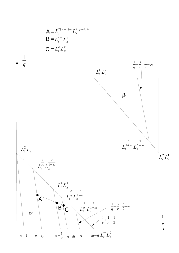
Figure 1. The Strichartz graph

5. Proof of Theorem

In this section, we prove Theorem 1.1.
The proof of Theorem 1.1 relies upon several propositions such as local boundedness, separation of the localized mollified energy, perturbation argument, and small mollified energy theory. We shall prove these propositions in Section 6, 7, 8, and 9.

5.1. Propositions

We consider $J$, $J^{\prime}$, and $\bar{J}^{{}^{\prime}}$ three intervals

$$J:=[a,b]\subset[0,\infty);\,\bar{J}^{{}^{\prime}}\subset J^{\prime}\subset J\cdot$$

Let $w$ be a solution of (1.1).

We assume that there exist $L_{w}$, $X_{w}$ such that

(5.1) $$\sup_{t\in J}E(Iw(t))\leq X_{w}\lesssim A^{p+1},$$

and

(5.2) $$\|Iw\|_{L_{t}^{2(p-1)-}L_{x}^{2(p-1)+}(J)}\leq L_{w}<\infty.$$

We will prove in Subsection 5.2 that these assumptions are always true.

Under these assumptions, one can find constants $\alpha_{1}$ and $c_{1}$ such that if

(5.3) $$\frac{\langle L_{w}\rangle^{\alpha_{1}}A^{\alpha_{1}}}{N^{(1-s_{c})-}}\leq c_{1},$$

then three propositions hold.
The first proposition shows that if $\bar{J}^{{}^{\prime}}$ is small in the sense of (5.4), then one can control several norms on this subinterval:

Proposition 5.1.

“Local boundedness” There exists a constant $c_{2}$ such that if

(5.4) $$\begin{array}[]{ll}\|Iw\|_{L_{t}^{2(p-1)-}L_{x}^{2(p-1)+}(\bar{J}^{{}^{\prime}})}\leq c_{2},\end{array}$$

then

(5.5) $$\begin{array}[]{ll}Z(\bar{J}^{{}^{\prime}},w)\lesssim X^{\frac{1}{2}}_{w}.\end{array}$$

The second proposition shows that if a subinterval is too large in the sense of (5.6), then one can separate the mollified energy into into two parts: one that is carried by a free Klein-Gordon solution and the other one that is carried by another solution $w^{\prime}$ of (1.1). The proof of Proposition 5.2 relies upon the combination of the $I$-method with a modification of arguments from Bourgain [1], or, more closely, Nakanishi [18, 19].

Proposition 5.2.

“ Separation of the localized mollified energy” Let $M\gg 1$. There exist $T\in J^{{}^{\prime}}$, and $v$, a solution of the free Klein-Gordon equation, and constants $c_{3}$, $C_{1}$, $C_{2}$, $\alpha_{2}$,…, $\alpha_{5}$ such that if

(5.6) $$\|Iw\|_{L_{t}^{2(p-1)-}L_{x}^{2(p-1)+}(J^{{}^{\prime}})}\geq C_{1}^{(C_{1}^{A^{\alpha_{2}}}M)^{C_{1}A^{\alpha_{2}}}},$$

then

(5.7) $$E_{c}(Iv) \lesssim 1,$$

(5.8) $$E(Iw^{\prime}(T)) \leq\sup_{t\in J^{{}^{\prime}}}E(Iw(t))-c_{3}A^{-\alpha_{3}},$$

(5.9) $$\text{and}\quad\|Iv\|_{L_{t}^{2(p-1)-}L_{x}^{2(p-1)+}(J^{\prime\prime})} \leq C_{2}\frac{A^{\alpha_{4}}}{M^{\alpha_{5}}},\quad\text{for}\quad J^{\prime\prime}:=(T,b)\quad\text{or}\quad\text{for}\quad J^{\prime\prime}:=(a,T).$$

Here $w^{\prime}$ denotes the solution of (1.1) such that $w^{\prime}(T):=w(T)-v(T)$.

The third proposition shows that if the target norm of $v$ is small in the sense of (5.11), then the target norm of $w$ can be estimated from that of $w^{\prime}$ :

Proposition 5.3.

“Perturbation argument” Let $T$, $v$, and $w^{\prime}$ be defined in the previous proposition. Let $J^{\prime\prime}:=(T,b)$ (or $J^{\prime\prime}:=(a,T)$). Assume that $w^{\prime}$ satisfies (5.1) and (5.2) (with $w$ substituted for $w^{\prime}$). Then there exist $c_{4}$, $C_{3}$, $C_{4}$, $\alpha_{6}$, $\alpha_{7}$, $\alpha_{8}$, and $k$ such that if

(5.10) $$\frac{C_{3}^{(A\langle L_{w^{\prime}}\rangle)^{\alpha_{6}}}(A\langle L_{w}\rangle)^{\alpha_{6}}}{N^{(1-s_{c})-}}\leq c_{4},$$

(5.11) $$k\leq\frac{1}{C_{4}^{(A\langle L_{w^{\prime}}\rangle)^{\alpha_{7}}}}\quad\text{and}\quad\|Iv\|_{L_{t}^{2(p-1)-}L_{x}^{2(p-1)+}(J^{\prime\prime})}\leq k,$$

then

(5.12) $$\|Iw\|_{L_{t}^{2(p-1)-}L_{x}^{2(p-1)+}(J^{\prime\prime})}\lesssim\left(\langle L_{w^{\prime}}\rangle A\right)^{\alpha_{8}}.$$

Next we show that if the mollified energy is small enough at one time, then we can have a very good control of the mollified energy and our target norm:

Proposition 5.4.

“ Small mollified energy theory”

Assume that there exists $\tilde{t}\in\mathbb{R}$ such that

(5.13) $$E(Iw(\tilde{t}))\ll 1.$$

Then one can find constants $\alpha_{9}$ and $c_{5}$ such that if

(5.14) $$\frac{A^{\alpha_{9}}}{N^{(1-s_{c})-}}\leq c_{5},$$

then

(5.15) $$\|Iw\|_{L_{t}^{2(p-1)-}L_{x}^{2(p-1)+}(\mathbb{R})}\lesssim 1,$$

and there exist $c_{6}$ and $\alpha_{10}$ such that

(5.16) $$\sup_{t\in\mathbb{R}}E(Iw(t))\leq E(Iw(\tilde{t}))(1+c_{6}A^{-\alpha_{10}}).$$

In fact, one can choose $c_{6}$ (resp. $\alpha_{10}$) arbitrarily small (resp. arbitrarily large) in (5.16), by choosing $c_{5}$ (resp. $\alpha_{9}$) small enough (resp. large enough) in (5.14).

5.2. The proof

We are now in position to prove Theorem 1.1. We define the following statement of induction for $l\in\mathbb{N}$

$\mathcal{P}(l)$: let

$$\mathcal{C}_{l}:=\left\{\begin{array}[]{ll}w_{l},\begin{array}[]{l}w_{l}\quad\text{solution}\quad\text{of}\quad(\ref{Eqn:NlkgWdat}),\\ \exists\,t_{l}\in\mathbb{R}^{+}\quad s.t\quad E(Iw_{l}(t_{l}))\leq C_{in,2}A^{p+1}-0.9lc_{3}A^{-\alpha_{3}};\end{array}\end{array}\right\},$$

then there exists $\infty>L(l):=L_{N,s,A}(l)$ such that

(5.17) $$\inf\{\bar{C},\,w_{l}\in\mathcal{C}_{l}\quad\text{and}\quad\|Iw_{l}\|_{L_{t}^{2(p-1)-}L_{x}^{2(p-1)+}(\mathbb{R}^{+})}\leq\bar{C}\}=L(l)$$

and

(5.18) $$\sup_{t\in\mathbb{R}^{+}}E(Iw_{l}(t))\leq(C_{in,2}A^{p+1}-0.9lc_{3}A^{-\alpha_{3}})(1+c_{6}A^{-\alpha_{10}}).$$

We easily obtain that $\mathcal{P}(\bar{l})$ holds for some $\bar{l}\lesssim A^{p+1+\alpha_{3}}$ by applying Proposition 5.4, choosing $N$ such that (5.14) holds.

Our goal is then to show that if $\mathcal{P}(l+1)$ holds, then $\mathcal{P}(l)$ also holds for $N$ and $s$ to be properly chosen. To this end let $w_{l}\in\mathcal{C}_{l}$. Let $T>0$. Assume that (5.17) restricted to $[0,t_{l}+T]$ holds for some $L(l)<\infty$ to be chosen. Choose $N$ such that (5.3), (5.10), and (5.14) hold with $L_{w}$, $L_{w^{\prime}}$ substituted respectively for $L(l)$, $L(l+1)$. Clearly (5.10) is the most constraining assumption to satisfy, choosing $C_{3}$ and $\alpha_{6}$ (resp. $c_{4}$) large enough (resp. small enough). One may partition $[0,t_{l}+T]$ into subintervals $J$ such that $\|Iw_{l}\|_{L_{t}^{2(p-1)-}L_{x}^{2(p-1)+}(J)}=c_{2}$ (except maybe the last one), one may apply Proposition 5.1 and Proposition 3.3 on each $J$, and then one may iterate to get for $t\in[0,t_{l}+T]$

$$\begin{array}[]{ll}\left|E(Iw_{l}(t))-E(Iw_{l}(t_{l}))\right|&\lesssim\frac{(C_{in,2}A^{p+1}-0.9lc_{3}A^{-\alpha_{3}})^{\frac{p+1}{2}}\langle L(l)\rangle^{2(p-1)-}}{N^{\frac{5-p}{2}-}}\\ &\leq c_{6}A^{-\alpha_{10}}\left(C_{in,2}A^{p+1}-0.9lc_{3}A^{-\alpha_{3}}\right),\end{array}$$

using (5.3), and choosing $\alpha_{1}$ (resp. $c_{1}$) large (resp. small) enough. Therefore (5.18) holds. It remains to prove (5.17). To this end we let $M$ be such that

(5.19) $$C_{2}\frac{A^{\alpha_{4}}}{M^{\alpha_{5}}}=\frac{1}{C_{4}^{(A\langle L(l+1)\rangle)^{\alpha_{7}}}},$$

Let $B>0$. If $\|Iw_{l}\|_{L_{t}^{2(p-1)-}L_{x}^{2(p-1)+}([0,t_{l}+T])}\geq 3B$, then we can find $(\overline{t}_{l},\overline{\overline{t}}_{l})\in[0,t_{l}+T]^{2}$ such that

$$\|Iw_{l}\|_{L_{t}^{2(p-1)-}L_{x}^{2(p-1)+}([0,\overline{t}_{l}])}\geq B,\quad\|Iw_{l}\|_{L_{t}^{2(p-1)-}L_{x}^{2(p-1)+}([\overline{t}_{l},\overline{\overline{t}}_{l}])}\geq B,\quad\text{and}\quad\|Iw_{l}\|_{L_{t}^{2(p-1)-}L_{x}^{2(p-1)+}([\overline{\overline{t}}_{l},t_{l}+T])}\geq B.$$

Assume that $B\geq C_{1}^{(C_{1}^{A^{\alpha_{2}}}M)^{C_{1}A^{\alpha_{2}}}}$. Then, applying Proposition 5.2 to $J^{\prime}:=[\overline{t}_{l},\overline{\overline{t}}_{l}]$, we see that there exists $T_{l}\in J^{{}^{\prime}}$ and $w^{{}^{\prime}}_{l}$ solution of (1.1) such that

$$E(Iw^{{}^{\prime}}_{l},T_{l}) \leq(C_{in,2}A^{p+1}-0.9lc_{3}A^{-\alpha_{3}})(1+c_{6}A^{-\alpha_{10}})-c_{3}A^{-\alpha_{3}}$$

(5.20) $$\leq C_{in,2}A^{p+1}-0.9(l+1)c_{3}A^{-\alpha_{3}},$$

choosing $c_{6}$ (resp. $\alpha_{10}$) small (resp. large) enough. Therefore $w^{{}^{\prime}}_{l}\in\mathcal{C}_{l+1}$. We deal with the case where (5.9) holds with $J^{\prime\prime}:=[T_{l},t_{l}+T]$ . Applying $\mathcal{P}(l+1)$ and Proposition 5.12, we see that

$$B\leq\|Iw_{l}\|_{L_{t}^{2(p-1)-}L_{x}^{2(p-1)+}([\overline{\overline{t}}_{l},t_{l}+T])}\leq\|Iw_{l}\|_{L_{t}^{2(p-1)-}L_{x}^{2(p-1)+}([T_{l},t_{l}+T])}\lesssim\left(\langle L(l+1)\rangle A\right)^{\alpha_{8}}.$$

Therefore we see that $\|Iw_{l}\|_{L_{t}^{2(p-1)-}L_{x}^{2(p-1)+}([0,t_{l}+T])}<\infty$, $\mathcal{P}(l)$ holds, and, moreover, there exist $\alpha\gtrsim 1$ and $C\gtrsim 1$ such that

(5.21) $$L(l)\lesssim\max\left(C_{1}^{(C_{1}^{A^{\alpha_{2}}}C_{2}^{\frac{1}{\alpha_{5}}}A^{\frac{\alpha_{4}}{\alpha_{5}}}C_{4}^{\frac{(A\langle L(l+1)\rangle)^{\alpha_{7}}}{\alpha_{5}}})^{C_{1}A^{\alpha_{2}}}},(\langle L(l+1)\rangle A)^{\alpha_{8}}\right)\leq C^{C^{\max^{\alpha}(A,\langle L(l+1)\rangle)^{C\max^{\alpha}(A,\langle L(l+1)\rangle)}}}.$$

Iterating (5.21) $\bar{l}$ times, we see that for $0\leq l\leq\bar{l}$ (even if it means increasing the value of $\alpha$ and $C$)

$$L(l)\leq\|L\|_{\infty}:=C^{C^{...^{C^{\alpha}}}},$$

where the height of the tower is $\sim A^{\alpha}$. Such an iteration is possible if $\frac{C_{3}^{(A\langle\|L\|_{\infty}\rangle)^{\alpha_{6}}}(A\langle\|L\|_{\infty}\rangle)^{\alpha_{6}}}{N^{(1-s_{c})-}}\leq c_{4}$. Pick $N$ such that $\frac{c_{4}}{2}\leq\frac{C_{3}^{(A\langle\|L\|_{\infty}\rangle)^{\alpha_{6}}}(A\langle\|L\|_{\infty}\rangle)^{\alpha_{6}}}{N^{(1-s_{c})-}}\leq c_{4}$. From (2.1), we see that there exists $\tilde{s}$ such that $\mathcal{P}(l)$ holds for $1>s>\tilde{s}$. Moreover $\tilde{s}$ can be chosen to be of the form (1.7) as $A\rightarrow\infty$.

Global existence

From $\mathcal{P}(0)$ and (3.3) we see that solutions of (1.1) with $1>s>\tilde{s}$ and with data $(u_{0},u_{1})\in H^{s}\times H^{s-1}$ satisfying (1.6) satisfy

(5.22) $$\sup_{t\in\mathbb{R^{+}}}E(Iu(t))\lesssim A^{p+1},\quad\text{and}\quad\|Iu\|_{L_{t}^{2(p-1)-}L_{x}^{2(p-1)+}(\mathbb{R^{+}})}<\infty.$$

By time reversal symmetry, we may extend $\mathbb{R}^{+}$ to $\mathbb{R}$. By Plancherel, we have for all time $T\in\mathbb{R}$ $\|(u(T),\partial_{t}u(T))\|^{2}_{H^{s}\times H^{s-1}}\lesssim A^{p+1}$. This proves global well-posedness.

Global estimates

Now we claim that

(5.23) $$Z_{m,s}(\mathbb{R},u)\lesssim_{A}1$$

for all $0\leq m\leq s$. Indeed, by (5.22), we may divide $[0,\infty)$ in subintervals $J:=[a,b]$ such that $\|Iu\|_{L_{t}^{2(p-1)-}L_{x}^{2(p-1)+}(J)}=c_{2}$ (except maybe the last one). Moreover, plugging $\langle D\rangle^{1-m}I$ into (3.2), and by (5.22), we have

(5.24) $$\begin{array}[]{ll}Z_{m,s}(J,u)&\lesssim\left\|(\langle D\rangle Iu(a),\partial_{t}Iu(a))\right\|_{L^{2}\times L^{2}}+\left\|\langle D\rangle^{1-m}I(|u|^{p-1}u)\right\|_{L_{t}^{\frac{2}{1+m}}L_{x}^{\frac{2}{2-m}}(J)}\\ &\lesssim A^{\frac{p+1}{2}}+\left\|\langle D\rangle^{1-m}Iu\right\|_{L_{t}^{\frac{2}{m}+}L_{x}^{\frac{2}{1-m}-}(J)}\left\||u|^{p-1}\right\|_{L_{t}^{2-}L_{x}^{2+}(J)}\\ &\lesssim A^{\frac{p+1}{2}}+Z_{m,s}(J,u)\left(\|P_{\ll N}u\|^{p-1}_{L_{t}^{2(p-1)-}L_{x}^{2(p-1)+}(J)}+\|P_{\gtrsim N}u\|^{p-1}_{L_{t}^{2(p-1)-}L_{x}^{2(p-1)+}(J)}\right)\\ &\lesssim A^{\frac{p+1}{2}}+Z_{m,s}(J,u)\left(\|Iu\|^{p-1}_{L_{t}^{2(p-1)-}L_{x}^{2(p-1)+}(J)}+\frac{\|\langle D\rangle^{1-s_{c}}Iu\|^{p-1}_{L_{t}^{2(p-1)-}L_{x}^{2(p-1)+}(J)}}{N^{\frac{5-p}{2}-}}\right)\\ &\lesssim A^{\frac{p+1}{2}}+Z_{m,s}(J,u)\left(c_{2}^{p-1}+\frac{Z^{p-1}_{s_{c},s}(u,J)}{N^{\frac{5-p}{2}-}}\right)\\ \end{array}$$

By our choice of $N$, we have $\frac{A^{\frac{p(p+1)}{2}}}{N^{\frac{5-p}{2}-}}\ll A^{\frac{p+1}{2}}$. Therefore a continuity argument (first for $m=s_{c}$, then for the other $m$), we see that $Z_{m,s}(J,u)\lesssim A^{\frac{p+1}{2}}$. Iterating over $J$, we get (5.23).

Scattering

Let $\mathbf{v}(t):=\left(u(t),\,\partial_{t}u(t)\right)$, $\mathbf{v}_{0}:=\left(u_{0},\,u_{1}\right)$ and

$$\mathbf{u_{nl}}(t):=\left(\begin{array}[]{l}-\int_{0}^{t}\frac{\sin{\left((t-t^{{}^{\prime}})\langle D\rangle\right)}}{\langle D\rangle}\left(|u|^{p-1}(t^{{}^{\prime}})u(t^{{}^{\prime}})\right)\,dt^{{}^{\prime}}\\ \\ -\int_{0}^{t}\cos{\left((t-t^{{}^{\prime}})\langle D\rangle\right)}\left(|u|^{p-1}(t^{{}^{\prime}})u(t^{{}^{\prime}})\right)\,dt^{{}^{\prime}}\end{array}\right)\,.$$

Then we get from (1.2) $\mathbf{v}(t)=K(t)\mathbf{v_{0}}+\mathbf{u_{nl}}(t)$. Recall that the solution $u$ scatters in $H^{s}\times H^{s-1}$ if there exists $\mathbf{v_{+,0}}:=(u_{+,0},u_{+,1})$ such that $\left\|\mathbf{v}(t)-K(t)\mathbf{v_{+,0}}\right\|_{H^{s}\times H^{s-1}}\rightarrow 0$ as $t\rightarrow\infty$. In other words, since $K$ is bounded on $H^{s}\times H^{s-1}$, it suffices to prove that the quantity $\left\|K^{-1}(t)\mathbf{v}(t)-\mathbf{v_{+,0}}\right\|_{H^{s}\times H^{s-1}}\rightarrow 0$ as $t\rightarrow\infty$. A computation shows that

$$K^{-1}(t)=\left(\begin{array}[]{cc}\cos{(t\langle D\rangle)}&-\frac{\sin{(t\langle D\rangle)}}{\langle D\rangle}\\ &\\ \langle D\rangle\sin{(t\langle D\rangle)}&\cos{(t\langle D\rangle)}\end{array}\right)\,.$$

But $K^{-1}(t)\mathbf{v}(t)=\mathbf{v_{0}}-K^{-1}(t)\mathbf{u_{nl}}(t)$ and, by dualizing the Strichartz estimate $\|e^{it\langle D\rangle}f\|_{L_{t}^{\frac{2}{1-s}}L_{x}^{\frac{2}{1+s}}}\lesssim\|f\|_{H^{1-s}}$ (see Proposition 3.1), we have

$$\|K^{-1}(t_{1})\mathbf{u_{nl}}(t_{1})-K^{-1}(t_{2})\mathbf{u_{nl}}(t_{2})\|_{H^{s}\times H^{s-1}} \lesssim\||u|^{p-1}u\|_{L_{t}^{\frac{2}{1+s}}L_{x}^{\frac{2}{2-s}}([t_{1},\,t_{2}])}$$

$$\lesssim\|\langle D\rangle^{1-s}I\left(|u|^{p-1}u\right)\|_{L_{t}^{\frac{2}{1+s}}L_{x}^{\frac{2}{2-s}}([t_{1},\,t_{2}])}\,.$$

But, plugging $\langle D\rangle^{1-s}I$ into (3.2) and modifying slightly (5.24), we get

$$\left\|\langle D\rangle^{1-s}I(|u|^{p-1}u)\right\|_{L_{t}^{\frac{2}{1+s}}L_{x}^{\frac{2}{2-s}}([t_{1},t_{2}])} \lesssim Z_{s,s}([t_{1},t_{2}],u)\left(\|Iu\|^{p-1}_{L_{t}^{2(p-1)-}L_{x}^{2(p-1)+}([t_{1},t_{2}])}+\frac{Z^{p-1}_{s_{c},s}([t_{1},t_{2}],u)}{N^{\frac{5-p}{2}-}}\right).$$

Therefore, from (5.22) and (5.23), we see that the Cauchy criterion is satisfied by $K^{-1}(t)v(t)$ and we conclude that $K^{-1}(t)v(t)$ has a limit in $H^{s}\times H^{s-1}$ as $t$ goes to infinity. Moreover $\lim\limits_{t\rightarrow\infty}\left\|\mathbf{v}(t)-K(t)\mathbf{v_{+,0}}\right\|_{H^{s}\times H^{s-1}}=0$, with $\mathbf{v_{+,0}}:=\left(u_{+,0},u_{+,1}\right)$ given explicitly by

$$u_{+,0} :=u_{0}+\int_{0}^{\infty}\frac{\sin{(t^{{}^{\prime}}\langle D\rangle)}}{\langle D\rangle}\left(|u|^{p-1}(t^{{}^{\prime}})u(t^{{}^{\prime}})\right)\,dt^{{}^{\prime}},$$

$$u_{+,1} :=u_{1}-\int_{0}^{\infty}\cos{(t^{{}^{\prime}}\langle D\rangle)}\left(|u|^{p-1}(t^{{}^{\prime}})u(t^{{}^{\prime}})\right)\,dt^{{}^{\prime}}\,.$$

6. Proof of local boundedness

In this section we prove Proposition 5.1. Plugging $\langle D\rangle^{1-m}I$ into (3.2), we have (with $\bar{J}^{\prime}:=[\bar{a}^{\prime},\bar{b}^{\prime}]$)

(6.1) $$Z_{m,s}(J^{{}^{\prime}},w)\lesssim\|\langle D\rangle Iw(\bar{a}^{\prime})\|_{L^{2}}+\|\partial_{t}Iw(\bar{a}^{\prime})\|_{L^{2}}+\|\langle D\rangle^{1-m}I(|w|^{p-1}w)\|_{L_{t}^{\frac{2}{1+m}}L_{x}^{\frac{2}{2-m}}(\bar{J}^{{}^{\prime}})},$$

by (5.1). There are three cases:

• $m\leq s$. By slightly modifying (5.24)

  $$Z_{m,s}(\bar{J}^{{}^{\prime}},w) \lesssim X^{\frac{1}{2}}_{w}+Z_{m,s}(\bar{J}^{{}^{\prime}},w)\left(\|Iw\|^{p-1}_{L_{t}^{2(p-1)-}L_{x}^{2(p-1)+}(\bar{J}^{{}^{\prime}})}+\frac{\|\langle D\rangle^{1-s_{c}}Iw\|^{p-1}_{L_{t}^{2(p-1)-}L_{x}^{2(p-1)+}(\bar{J}^{{}^{\prime}})}}{N^{\frac{5-p}{2}-}}\right)$$

  $$\lesssim X^{\frac{1}{2}}_{w}+Z_{m,s}(\bar{J}^{{}^{\prime}},w)\left(c_{2}^{p-1}+\frac{Z^{p-1}_{s_{c},s}(\bar{J}^{{}^{\prime}},w)}{N^{\frac{5-p}{2}-}}\right)$$

  Again, choosing $\alpha_{1}$ (resp. $c_{1}$) large enough (resp. small enough) in (5.3), we have $\frac{A^{\frac{p(p+1)}{2}}}{N^{\frac{5-p}{2}-}}<<A^{\frac{p+1}{2}}$. Therefore a continuity argument (first for $m=s_{c}$, then for the other $m$) shows that $Z_{m,s}(\bar{J}^{{}^{\prime}},w)\lesssim X^{\frac{1}{2}}_{w}$.
  

• $m=1$. We estimate

  $$Z_{m,s}(\bar{J}^{{}^{\prime}},w) \lesssim X^{\frac{1}{2}}_{w}+\|I(|w|^{p-1}w)\|_{L_{t}^{1}L_{x}^{2}(\bar{J}^{{}^{\prime}})}$$

  $$\lesssim X^{\frac{1}{2}}_{w}+\||w|^{p-1}w\|_{L_{t}^{1}L_{x}^{2}(\bar{J}^{{}^{\prime}})}$$

  $$\lesssim X^{\frac{1}{2}}_{w}+\||P_{\ll N}w|^{p-1}P_{\ll N}w\|_{L_{t}^{1}L_{x}^{2}(\bar{J}^{{}^{\prime}})}+\||P_{\ll N}w|^{p-1}P_{\gtrsim N}w\|_{L_{t}^{1}L_{x}^{2}(\bar{J}^{{}^{\prime}})}$$

  $$+\||P_{\gtrsim N}w|^{p-1}P_{<<N}w\|_{L_{t}^{1}L_{x}^{2}(\bar{J}^{{}^{\prime}})}+\||P_{\gtrsim N}w|^{p-1}P_{\gtrsim N}w\|_{L_{t}^{1}L_{x}^{2}(\bar{J}^{{}^{\prime}})}$$

  $$\lesssim X^{\frac{1}{2}}_{w}+B_{1}+B_{2}+B_{3}+B_{4}\,.$$

  We estimate

  $$B_{1} \lesssim\|Iw\|^{p-1}_{L_{t}^{2(p-1)-}L_{x}^{2(p-1)+}(\bar{J}^{{}^{\prime}})}\|Iw\|_{L_{t}^{2+}L_{x}^{\infty-}(\bar{J}^{{}^{\prime}})}$$

  $$\lesssim c_{2}^{p-1}Z_{1,s}(w,\bar{J}^{{}^{\prime}}),$$

  $$B_{2} \lesssim\|Iw\|^{p-1}_{L_{t}^{p-1}L_{x}^{\frac{6(p-1)}{p-3}}(\bar{J}^{{}^{\prime}})}\|P_{\gtrsim N}w\|_{L_{t}^{\infty}L_{x}^{\frac{6}{6-p}}(\bar{J}^{{}^{\prime}})}$$

  $$\lesssim Z^{p-1}_{1,s}(\bar{J}^{{}^{\prime}},w)\frac{\|\langle D\rangle Iw\|_{L_{t}^{\infty}L_{x}^{2}(\bar{J}^{{}^{\prime}})}}{N^{\frac{5-p}{2}-}}$$

  $$\lesssim\frac{Z^{p-1}_{1,s}(\bar{J}^{{}^{\prime}},w)}{N^{\frac{5-p}{2}-}}X_{w}^{\frac{1}{2}},$$

  $$B_{3} \lesssim\frac{\|\langle D\rangle^{1-s_{c}}Iw\|^{p-1}_{L_{t}^{2(p-1)-}L_{x}^{2(p-1)+}(\bar{J}^{{}^{\prime}})}}{N^{\frac{5-p}{2}-}}\|Iw\|_{L_{t}^{2+}L_{x}^{\infty-}(\bar{J}^{{}^{\prime}})}$$

  $$\lesssim\frac{Z^{p-1}_{s_{c},s}(\bar{J}^{{}^{\prime}},w)}{N^{\frac{5-p}{2}-}}Z_{1,s}(\bar{J}^{{}^{\prime}},w)\lesssim\frac{X_{w}^{\frac{p-1}{2}}}{N^{\frac{5-p}{2}-}}Z_{1,s}(\bar{J}^{{}^{\prime}},w),$$

  $$B_{4} \lesssim\|P_{\gtrsim N}w\|^{p}_{L_{t}^{p}L_{x}^{2p}(\bar{J}^{{}^{\prime}})}\lesssim\frac{\|\langle D\rangle^{1-\left(\frac{3p-5}{2p}\right)}Iw\|^{p}_{L_{t}^{p}L_{x}^{2p}(\bar{J}^{{}^{\prime}})}}{N^{\frac{5-p}{2}-}}$$

  $$\lesssim\frac{Z^{p}_{\frac{3p-5}{2p},s}(\bar{J}^{{}^{\prime}},w)}{N^{\frac{5-p}{2}-}}\lesssim\frac{X_{w}^{\frac{p}{2}}}{N^{\frac{5-p}{2}-}}\,.$$

  Therefore, since again $N$ satisfies (5.3), we see by a continuity argument that $Z_{1,s}(\bar{J}^{{}^{\prime}},w)\lesssim X^{\frac{1}{2}}_{w}$.

• $s<m<1$: $Z_{m,s}(J^{{}^{\prime}},w)\lesssim X^{\frac{1}{2}}_{w}$ follows by interpolating between $m=s$ and $m=1$.

7. Proof of separation of the localized mollified energy

In this section we prove Proposition 5.2. The proof of Proposition 5.2 relies upon three lemmas that we show in the next subsections.

7.1. Lemmas 7.1, 7.2, and 7.3

The first lemma shows that if there is concentration of the target norm of the solution on a subinterval of $J^{{}^{\prime}}$ in the sense of (7.1), then this also means that the potential term of the mollified energy and the size of this subinterval are substantial.

Lemma 7.1.

Assume that

(7.1) $$\|Iw\|_{L_{t}^{2(p-1)-}L_{x}^{2(p-1)+}(\bar{J}^{{}^{\prime}})}=c_{2}.$$

Then there exist a subinterval $\bar{K}^{{}^{\prime}}\subset\bar{J}^{{}^{\prime}}$, a number $R\geq 1$, a point $\bar{x}^{{}^{\prime}}\in\mathbb{R}^{3}$ and constants $C_{5}$, $c_{7}$, $c_{8}$, $\alpha_{11}$,…, $\alpha_{13}$ such that

(7.2) $$\begin{array}[]{ll}R:=C_{5}A^{\alpha_{11}},\,|\bar{K}^{{}^{\prime}}|&=c_{7}A^{-\alpha_{12}},\end{array}$$

and for all $t\in\bar{K}^{{}^{\prime}}$

(7.3) $$\int_{|x-\bar{x}^{{}^{\prime}}|\leq R}|Iw(t,x)|^{p+1}\,dx\geq c_{8}A^{-\alpha_{13}}.$$

The second lemma shows that if we consider a partition of $J^{\prime}$ into subintervals where the target norm of the solution concentrates, then these subintervals must be large on average. In order to prove this lemma, we shall mostly use the previous lemma and the Almost Morawetz-Strauss estimate (3.5).

Lemma 7.2.

Let $(\bar{J}^{{}^{\prime}}_{j}=[\bar{a}^{{}^{\prime}}_{j},\bar{a}^{{}^{\prime}}_{j+1}])_{1\leq j\leq\bar{j}}$ be a partition of $J^{{}^{\prime}}$ such that $\|Iw\|_{L_{t}^{2(p-1)-}L_{x}^{2(p-1)+}(\bar{J}^{{}^{\prime}}_{j})}=c_{2}$, except maybe the last one. Then there exist $\bar{t}^{{}^{\prime}}_{j}\in\bar{J}^{{}^{\prime}}_{j}$ and a constant $\alpha_{14}$ such that

(7.4) $$\sum_{j=1}^{\bar{j}-1}\frac{1}{\bar{t}^{{}^{\prime}}_{j}+1}\lesssim A^{\alpha_{14}}.$$

The third lemma shows that if the target norm of the solution is too large in the sense of (7.5) then we can find a large subinterval where some norms are small compare with the concentration of mollified energy in the sense of (7.6)

Lemma 7.3.

Let $M\geq 1$. Then, there exist $C_{6}$, $c_{9}$, $\alpha_{15}$, and $\alpha_{16}$ for all $0<\epsilon\leq 1$, there exist $R^{{}^{\prime}}\in(1,\infty)$, $\bar{x}\in\mathbb{R}^{3}$ and $J^{\prime\prime}:=[S,T]$ (or $J^{\prime\prime}:=[T,S]$) such that $J^{\prime\prime}\subset J^{{}^{\prime}}$ and if

(7.5) $$\|Iw\|_{L_{t}^{2(p-1)-}L_{x}^{2(p-1)+}(J^{{}^{\prime}})}\geq C_{6}^{(C_{6}^{(A\epsilon^{-1})^{\alpha_{15}}}M)^{C_{6}A^{\alpha_{15}}}},$$

then

(7.6) $$\tilde{Z}(J^{\prime\prime},w)\leq c_{9}A^{-\alpha_{16}}\leq E(Iw(S),B(\bar{x},R^{{}^{\prime}})),$$

(7.7) $$|J^{\prime\prime}|\geq MR^{{}^{\prime}},$$

and

(7.8) $$\left\|\frac{Iw(S)}{\langle x-\bar{x}\rangle}\right\|_{L^{2}}\leq\epsilon\,.$$

7.2. The proof

We may assume without loss of generality that $S<T$. We apply Lemma 7.3 with $\epsilon<<\min\left(A^{-\frac{\alpha_{16}}{2}},A^{-\alpha_{16}-\frac{p+1}{2}}\right)$. Notice that with this choice of $\epsilon$, the condition (7.5) becomes (5.6), choosing $\alpha_{2}$ large enough. The proof is made of several steps:

Step 1. Construction of the free Klein-Gordon equation $v$ and proof of (5.7).

Let $P(y):=\left\{y\in\mathbb{R}^{3},\,E\left(Iw(S),B(y,1)\right)\leq c_{9}A^{-\alpha_{16}}\right\}$. Then by (5.1) there exists $\bar{\bar{x}}\in\mathbb{R}^{3}$ such that $|\bar{x}-\bar{\bar{x}}|\lesssim A^{p+1+\alpha_{16}}$ and $P(\bar{\bar{x}})$ is true. Hence, using also (7.6) we see that there exists a constant $C$ and $\Gamma\in[\frac{1}{2},R^{{}^{\prime}}+CA^{p+1+\alpha_{16}}]$ such that

(7.9) $$E\left(Iw(S),B(\bar{\bar{x}},\Gamma)\right)=c_{9}A^{-\alpha_{16}}\,.$$

Let $v$ be the solution of the free Klein-Gordon equation with data

$$\begin{cases}v(S):=I^{-1}\left(\chi\left(\frac{x-\bar{\bar{x}}}{\Gamma}\right)Iw(S)\right)\\ \partial_{t}v(S):=I^{-1}\left(\chi\left(\frac{x-\bar{\bar{x}}}{\Gamma}\right)\partial_{t}Iw(S)\right),\end{cases}$$

where $\chi$ is a smooth function such that $\chi(x)=1$ if $|x|\leq 1$ and $\chi(x)=0$ if $|x|\geq 2$. By (5.1) and (7.8) we see that there exists a constant $C$ such that

$$E_{c}\left(Iv(S)\right) \leq E\left(Iw(S),B(\bar{\bar{x}},\Gamma)\right)+\frac{C}{\Gamma^{2}}\int_{\Gamma\leq|x-\bar{\bar{x}}|\leq 2\Gamma}|Iw(S)|^{2}\,dx+$$

(7.10) $$\frac{C}{\Gamma}\int_{\Gamma\leq|x-\bar{\bar{x}}|\leq 2\Gamma}|Iw(S)||\nabla Iw(S)|\,dx$$

$$\leq c_{9}A^{-\alpha_{16}}+CA^{\frac{p+1}{2}}\left\|\frac{Iw(S)}{\langle x-\bar{\bar{x}}\rangle}\right\|_{L^{2}}+C\left\|\frac{Iw(S)}{\langle x-\bar{\bar{x}}\rangle}\right\|^{2}_{L^{2}}$$

$$\lesssim A^{-\alpha_{16}},$$

Hence, using also the conservation of $E_{c}(Iv)$, we see that (5.7) holds.

Step 2. Proof of the decay (5.9).

By interpolation we see that one can choose one can choose $m<s_{c}$ close to $s_{c}$ and $\gamma>0$ close to zero such that

$$\|Iv\|_{L_{t}^{2(p-1)-}L_{x}^{2(p-1)+}(T,b)} \lesssim\|\langle D\rangle^{1-m}Iv\|^{1-\gamma}_{L_{t}^{\frac{8}{3-2m}-}L_{x}^{\frac{8}{3-2m}+}(T,b)}\|\langle D\rangle^{-\left(\frac{3}{2}++\right)}Iv\|^{\gamma}_{L_{t}^{\infty}L_{x}^{\infty}(T,b)}$$

$$\lesssim A^{-(1-\gamma)\alpha_{16}}\|Iv\|^{\gamma}_{L_{t}^{\infty}B_{\infty,2}^{-\left(\frac{3}{2}+\right)}(T,b)}$$

$$\lesssim A^{-(1-\gamma)\alpha_{16}}\frac{1}{|T-S|^{\frac{3\gamma}{2}}}\left(\|Iv(S)\|^{\gamma}_{B^{1-}_{1,2}}+\|\partial_{t}Iv(S)\|^{\gamma}_{B^{0-}_{1,2}}\right)$$

$$\lesssim A^{-(1-\gamma)\alpha_{16}}\frac{1}{|T-S|^{\frac{3\gamma}{2}}}\left(\Gamma^{\frac{3\gamma}{2}}\|Iw(S)\|^{\gamma}_{L^{2}}+\Gamma^{\frac{\gamma}{2}}\|\nabla Iw(S)\|^{\gamma}_{L^{2}}+\Gamma^{\frac{3\gamma}{2}}\|\partial_{t}Iw(S)\|^{\gamma}_{L^{2}}\right)$$

(7.11) $$\leq C_{2}\frac{A^{\alpha_{4}}}{M^{\alpha_{5}}},$$

using also (7.7), (7.10) combined with (3.2), and the following dispersive estimate (see [9], Lemma 2.1)

(7.12) $$\|e^{it\langle D\rangle}\phi\|_{B^{-\frac{5}{4}}_{\infty,2}}\lesssim\frac{1}{|t|^{\frac{3}{2}}}\|\phi\|_{B^{\frac{5}{4}}_{1,2}}.$$

Step 3. Proof of the separation of the localized mollified energy (5.8).

Let $\bar{w}:=w-v$. Then

$$E\left(I\bar{w}(S)\right) \leq\frac{1}{2}\int_{\mathbb{R}^{3}}\left(1-\chi^{2}\left(\frac{x-\bar{\bar{x}}}{\Gamma}\right)\right)|\nabla Iw(S)|^{2}\,dx$$

$$+\frac{1}{p+1}\int_{\mathbb{R}^{3}}\left(1-\chi^{p+1}\left(\frac{x-\bar{\bar{x}}}{\Gamma}\right)\right)|Iw(S)|^{p+1}\,dx$$

$$+\frac{1}{2}\int_{\mathbb{R}^{3}}\left(1-\chi^{2}\left(\frac{x-\bar{\bar{x}}}{\Gamma}\right)\right)|\partial_{t}Iw(S)|^{2}\,dx+\frac{1}{2}\int_{\mathbb{R}^{3}}\left(1-\chi^{2}\left(\frac{x-\bar{\bar{x}}}{\Gamma}\right)\right)|Iw(S)|^{2}\,dx$$

$$+\frac{C}{\Gamma}\int_{\Gamma\leq|x-\bar{\bar{x}}|\leq 2\Gamma}|Iw(S)||\nabla Iw(S)|\,dx+\frac{C}{\Gamma^{2}}\int_{\Gamma\leq|x-\bar{\bar{x}}|\leq 2\Gamma}|Iw(S)|^{2}\,dx$$

$$\leq\sup_{t\in J}E(Iw(t))-c_{9}A^{-\alpha_{16}}+CA^{\frac{p+1}{2}}\left\|\frac{Iw(S)}{\langle x-\bar{\bar{x}}\rangle}\right\|_{L^{2}}+C\left\|\frac{Iw(S)}{\langle x-\bar{\bar{x}}\rangle}\right\|^{2}_{L^{2}}$$

(7.13) $$\leq\sup_{t\in J}E(Iw(t))-\frac{c_{9}A^{-\alpha_{16}}}{2}\,.$$

Let

$$\bar{Z}([S,T],f):=\|If\|_{L_{t}^{2(p-1)-}L_{x}^{2(p-1)+}([S,T])}+\|\partial_{t}\langle D\rangle^{-\frac{1}{2}}If\|_{L_{t}^{4}L_{x}^{4}([S,T])}+\|\langle D\rangle^{\frac{1}{2}}If\|_{L_{t}^{4+}L_{x}^{4-}([S,T])}$$

Plugging $\langle D\rangle^{1-\frac{1}{2}}I$ into (3.2), we see, by (7.6) and the Sobolev embedding

$$\|If\|_{L_{t}^{2(p-1)-}L_{x}^{2(p-1)+}([S,T])}\lesssim\|\langle D\rangle^{1-\frac{1}{2}}If\|_{L_{t}^{2(p-1)-}L_{x}^{\frac{6(p-1)}{2p-3}+}([S,T])},$$

that

(7.14) $$\bar{Z}([S,T],\bar{w})\lesssim\left\|\langle D\rangle^{1-\frac{1}{2}}I(|w|^{p-1}w)\right\|_{L_{t}^{\frac{4}{3}}L_{x}^{\frac{4}{3}}([S,T])}$$

$$\lesssim\|\langle D\rangle^{1-\frac{1}{2}}Iw\|_{L_{t}^{4+}L_{x}^{4-}([S,T])}\left(\|P_{<<N}w\|^{p-1}_{L_{t}^{2(p-1)-}L_{x}^{2(p-1)+}([S,T])}+\|P_{\gtrsim N}w\|^{p-1}_{L_{t}^{2(p-1)-}L_{x}^{2(p-1)+}([S,T])}\right)$$

$$\lesssim\|\langle D\rangle^{1-\frac{1}{2}}Iw\|_{L_{t}^{4+}L_{x}^{4-}([S,T])}\left(\|Iw\|^{p-1}_{L_{t}^{2(p-1)-}L_{x}^{2(p-1)+}([S,T])}+\frac{\|\langle D\rangle^{1-\frac{1}{2}}Iw\|^{p-1}_{L_{t}^{2(p-1)-}L_{x}^{\frac{6(p-1)}{2p-3}+}([S,T])}}{N^{\frac{5-p}{2}-}}\right)$$

$$\lesssim\tilde{Z}^{p}([S,T],w)$$

$$\leq\frac{c_{9}A^{-\alpha_{16}}}{1000}.$$

We compute

$$\partial_{t}E(I\bar{w}) =\int_{\mathbb{R}^{3}}\Re\left(\overline{\partial_{t}I\bar{w}}\left(\partial_{tt}I\bar{w}-\triangle I\bar{w}+I\bar{w}+F(I\bar{w})\right)\right)\,dx$$

$$=\int_{\mathbb{R}^{3}}\Re\left(\overline{\partial_{t}I\bar{w}}(F(I\bar{w})-IF(w))\right)\,dx\,.$$

Now, we decompose $E(I\bar{w}(T))-E(I\bar{w}(S))=X_{1,1}+X_{1,2}+X_{2}$ where

$$X_{1,1} :=\int_{S}^{T}\int_{\mathbb{R}^{3}}\Re{\left(\overline{\partial_{t}I\bar{w}}\left(F(w)-IF(w)\right)\right)}\,dx\,dt\,$$

$$X_{1,2} :=\int_{S}^{T}\int_{\mathbb{R}^{3}}\Re{\left(\overline{\partial_{t}I\bar{w}}\left(F(Iw)-F(w)\right)\right)}\,dx\,dt$$

(7.15) $$X_{2} :=\int_{S}^{T}\int_{\mathbb{R}^{3}}\Re{\left(\overline{\partial_{t}I\bar{w}}\left(F(I\bar{w})-F(Iw)\right)\right)}\,dx\,dt.$$

We estimate $X_{2}$. From (7.6) and (7.14)

$$|X_{2}| \lesssim\|\partial_{t}\langle D\rangle^{-\frac{1}{2}}I\bar{w}\|_{L_{t}^{4}L_{x}^{4}([S,T])}\|\langle D\rangle^{\frac{1}{2}}(F(I\bar{w})-F(Iw))\|_{L_{t}^{\frac{4}{3}}L_{x}^{\frac{4}{3}}([S,T])}$$

$$\lesssim\|\partial_{t}\langle D\rangle^{-\frac{1}{2}}I\bar{w}\|_{L_{t}^{4}L_{x}^{4}([S,T])}\left(\|Iw\|^{p-1}_{L_{t}^{2(p-1)-}L_{x}^{2(p-1)+}([S,T])}+\|I\bar{w}\|^{p-1}_{L_{t}^{2(p-1)-}L_{x}^{2(p-1)+}([S,T])}\right)$$

$$\left(\|\langle D\rangle^{1-\frac{1}{2}}Iw\|_{L_{t}^{4+}L_{x}^{4-}([S,T])}+\|\langle D\rangle^{\frac{1}{2}}I\bar{w}\|_{L_{t}^{4+}L_{x}^{4-}([S,T])}\right)$$

$$\leq\frac{c_{9}A^{-\alpha_{16}}}{1000}.$$

Hence, using also (7.13) and Result 10.1 (see Appendix A) we see that (5.8) holds, with $w^{\prime}$ solution of (1.1) such that $w^{\prime}(T):=\bar{w}(T)$.

7.3. Proof of Lemma 7.1

The proof is made of four steps:

Step 1. Lower bound of the size of $\bar{J}^{{}^{\prime}}$.

We see from Proposition 5.1 that if $p\geq 4$, then

$$c_{2} =\|Iw\|_{L_{t}^{2(p-1)-}L_{x}^{2(p-1)+}(\bar{J}^{{}^{\prime}})}$$

$$\lesssim|\bar{J}^{{}^{\prime}}|^{\frac{5-p}{2(p-1)}+}\|\langle D\rangle^{1-\frac{1}{2}}Iw\|_{L_{t}^{\frac{2(p-1)}{p-4}}L_{x}^{\frac{6(p-1)}{p+2}}(\bar{J}^{{}^{\prime}})}$$

$$\lesssim|\bar{J}^{{}^{\prime}}|^{\frac{5-p}{2(p-1)}+}A^{\frac{p+1}{2}},$$

and if $p<4$, then

$$c_{2} =\|Iw\|_{L_{t}^{2(p-1)-}L_{x}^{2(p-1)+}(\bar{J}^{{}^{\prime}})}$$

$$\lesssim|\bar{J}^{{}^{\prime}}|^{\frac{1}{2(p-1)}+}\|\langle D\rangle^{1-\frac{1}{2}}Iw\|_{L_{t}^{\infty}L_{x}^{3}(\bar{J}^{{}^{\prime}})}$$

$$\lesssim|\bar{J}^{{}^{\prime}}|^{\frac{1}{2(p-1)}+}A^{\frac{p+1}{2}}\,.$$

Therefore, we conclude that there exists a constant $c$ such that

(7.16) $$|\bar{J}^{{}^{\prime}}|\geq c\times\left\{\begin{array}[]{l}A^{-\frac{(p+1)(p-1)}{5-p}+},\,p\geq 4\\ A^{-(p+1)(p-1)+},\,p<4\end{array}\right.$$

Step 2. Lower bound of $\|P_{M}w\|_{L_{t}^{\infty}L_{x}^{\infty}(\bar{J}^{{}^{\prime}})}$ for some $M\in 2^{\mathbb{N}}$

From Proposition 5.1

$$c_{2}= \|Iw\|_{L_{t}^{2(p-1)-}L_{x}^{2(p-1)+}(\bar{J}^{{}^{\prime}})}$$

$$\lesssim\|\langle D\rangle^{1-\left(\frac{1}{2}+\right)}Iw\|^{\frac{2}{p-1}}_{L_{t}^{4-}L_{x}^{4+}(\bar{J}^{{}^{\prime}})}\|\langle D\rangle^{\left(-\frac{1}{p-3}\right)+}Iw\|^{1-\frac{2}{p-1}}_{L_{t}^{\infty}L_{x}^{\infty}(\bar{J}^{{}^{\prime}})}$$

$$\lesssim A^{\frac{p+1}{p-1}}\|\langle D\rangle^{\left(-\frac{1}{p-3}\right)+}Iw\|^{1-\frac{2}{p-1}}_{L_{t}^{\infty}L_{x}^{\infty}(\bar{J}^{{}^{\prime}})}.$$

Thus we have $\|\langle D\rangle^{\left(-\frac{1}{p-3}\right)+}Iw\|_{L_{t}^{\infty}L_{x}^{\infty}(\bar{J}^{{}^{\prime}})}\gtrsim A^{-\frac{p+1}{p-3}}$ and, by the pigeonhole principle, we conclude that there exists $M\in 2^{\mathbb{N}}$ such that

(7.17) $$\|P_{M}Iw\|_{L_{t}^{\infty}L_{x}^{\infty}(\bar{J}^{{}^{\prime}})}\gtrsim\langle M\rangle^{\frac{1}{p-3}-}A^{-\frac{p+1}{p-3}}\,.$$

On the other hand,

(7.18) $$\|P_{M}Iw\|_{L_{t}^{\infty}L_{x}^{\infty}(\bar{J}^{{}^{\prime}})}\lesssim\langle M\rangle^{\frac{1}{2}}\|\langle D\rangle Iw\|_{L_{t}^{\infty}L_{x}^{2}(\bar{J}^{{}^{\prime}})}\lesssim\langle M\rangle^{\frac{1}{2}}A^{\frac{p+1}{2}}.$$

Combining (7.17) and (7.18), we see that

(7.19) $$\langle M\rangle\lesssim A^{\frac{(p+1)(p-1)}{5-p}+}\,.$$

Step 3. Control of $|P_{M}Iw(t,\bar{x}^{{}^{\prime}})|$ for some $\bar{x}^{{}^{\prime}}\in\mathbb{R}^{3}$ and for all $t\in\bar{K}^{{}^{\prime}}$, $\bar{K}^{{}^{\prime}}\subset\bar{J}^{{}^{\prime}}$ to be defined shortly.

By (7.17), there exists $(\bar{t}^{{}^{\prime}},\bar{x}^{{}^{\prime}})$ such that

(7.20) $$|P_{M}Iw(\bar{t}^{{}^{\prime}},\bar{x}^{{}^{\prime}})|\gtrsim\langle M\rangle^{\frac{1}{p-3}-}A^{-\frac{p+1}{p-1}}\,.$$

But, by (5.1) and (7.19), we see that

$$|P_{M}Iw(t,\bar{x}^{{}^{\prime}})-P_{M}Iw(\bar{t}^{{}^{\prime}},\bar{x}^{{}^{\prime}})| \lesssim\sup_{s\in(\bar{t}{{}^{\prime}},t)}\|\partial_{s}Iw(s)\|_{L_{x}^{2}}\langle M\rangle^{\frac{3}{2}}|t-\bar{t}^{{}^{\prime}}|$$

(7.21) $$\lesssim A^{\frac{(p+1)^{2}}{5-p}}|t-\bar{t}^{{}^{\prime}}|\,,$$

Therefore, in view of (7.16), (7.20) and (7.21), choosing $c_{7}$ (resp. $\alpha_{12}$) small enough (resp. large enough), we see that either $[\bar{t}^{{}^{\prime}},\bar{t}^{{}^{\prime}}+c_{7}A^{-\alpha_{12}}]\subset\bar{J}^{{}^{\prime}}$ (in this case we let $\bar{K}^{{}^{\prime}}:=[\bar{t}^{{}^{\prime}},\bar{t}^{{}^{\prime}}+c_{7}A^{-\alpha_{12}}]$), or $[\bar{t}^{{}^{\prime}}-c_{7}A^{-\alpha_{12}},\bar{t}^{{}^{\prime}}]\subset\bar{J}^{{}^{\prime}}$ (in this case we let $\bar{K}^{{}^{\prime}}:=[\bar{t}^{{}^{\prime}}-c_{7}A^{-\alpha_{12}},\bar{t}^{{}^{\prime}}]$ ) and

(7.22) $$|P_{M}Iw(t,\bar{x}^{{}^{\prime}})|\gtrsim A^{-\frac{p+1}{p-1}},\,t\in\bar{K}^{{}^{\prime}}$$

Step 4. Lower bound of potential mollified energy.

Let $R>0$ to be fixed shortly. Let $\Psi:=\psi$ if $M>1$ and $\Psi:=\phi$ is $M=1$. By (7.22) we have

$$M^{3}(B_{1}+B_{2})\gtrsim A^{-\frac{p+1}{p-1}}$$

where $B_{1}:=\int_{|y|\leq R}|\check{\Psi}(My)||Iw(t,\bar{x}^{{}^{\prime}}-y)|\,dy$ and $B_{2}:=\int_{|y|\geq R}|\check{\Psi}(My)||Iw(t,\bar{x}^{{}^{\prime}}-y)|\,dy$. We have

$$B_{1} \lesssim\left(\int_{|y|\leq R}|\check{\Psi}(My)|^{\frac{p+1}{p}}\,dy\right)^{\frac{p}{p+1}}\left(\int_{|y|\leq R}|Iw(t,\bar{x}^{{}^{\prime}}-y)|^{p+1}\,dy\right)^{\frac{1}{p+1}}$$

$$\lesssim\left(\int_{|y-\bar{x}^{{}^{\prime}}|\leq R}|Iw(t,y)|^{p+1}\,dy\right)^{\frac{1}{p+1}}M^{-\frac{3p}{p+1}}$$

and

$$B_{2} \lesssim M^{-\frac{3}{2}}\|\check{\Psi}\|_{L^{2}(|y|\geq MR)}\|Iw(t)\|_{L_{x}^{2}}$$

$$\lesssim M^{-\frac{3}{2}}\|\check{\Psi}\|_{L^{2}(|y|\geq MR)}A^{\frac{p+1}{2}}\,.$$

The fast decay of $\check{\Psi}$ implies

$$\|\check{\Psi}\|_{L^{2}(|y|\geq MR)}\lesssim\frac{1}{(MR)^{\frac{3}{2}}}.$$

Hence, if $R:=C_{5}A^{\alpha_{11}}$ (with $C_{5}$ and $\alpha_{11}$ large enough), then

$$\int_{|y-\bar{x}^{{}^{\prime}}|\leq R}|Iw(t,y)|^{p+1}\,dy\geq c_{8}A^{-\alpha_{13}},$$

for all $t\in\bar{K}^{{}^{\prime}}$.

7.4. Proof of Lemma 7.2

Let $j\in[1,\bar{j}-1]$. Recall that, by Lemma 7.1, on each $\bar{J}^{{}^{\prime}}_{j}$, there exist $\bar{x}^{{}^{\prime}}_{j}\in\mathbb{R}^{3}$ and $\bar{K}^{{}^{\prime}}_{j}=[\bar{t}^{{}^{\prime}}_{j},\bar{t}^{{}^{\prime}}_{j+1}]\subset\bar{J}^{{}^{\prime}}_{j}$ such that

(7.23) $$\int_{|x-\bar{x}^{{}^{\prime}}_{j}|\leq R}|Iw(t,x)|^{p+1}\,dx\geq c_{8}A^{-\alpha_{13}}$$

for all $t\in\bar{K}^{{}^{\prime}}_{j}$, with $R=C_{5}A^{\alpha_{11}}$ and

(7.24) $$|\bar{K}^{{}^{\prime}}_{j}|=c_{7}A^{-\alpha_{12}}.$$

We construct (see [18]) a set $\mathcal{P}:=\{j_{1},....,j_{l}\}\subset\{1,...,\bar{j}-1\}$. Initially $j_{1}=1$. Then let $j_{k+1}$ be the minimal $j$ such that

(7.25) $$|\bar{x}^{{}^{\prime}}_{j}-\bar{x}^{{}^{\prime}}_{j_{k+1}}|\geq|\bar{t}^{{}^{\prime}}_{j}-\bar{t}^{{}^{\prime}}_{j_{k+1}}|+100R$$

for $j:=j_{1},...,j_{k}$. Observe that $J^{{}^{\prime}}=\bigcup_{j_{k}\in\mathcal{P}}A^{{}^{\prime}}_{j_{k}}$ with

$$A^{{}^{\prime}}_{j_{k}}:=\left\{\bar{J}^{{}^{\prime}}_{l},\,\bar{j}-1\geq l\geq j_{k},\,and\,|\bar{x}^{{}^{\prime}}_{j_{k}}-\bar{x}^{{}^{\prime}}_{l}|<|\bar{t}^{{}^{\prime}}_{j_{k}}-\bar{t}^{{}^{\prime}}_{l}|+100R\right\}.$$

From Result 10.2 and the estimates above

$$A^{p+1}\operatorname{card}{\mathcal{P}} \gtrsim\sum_{j_{k}\in\mathcal{P}}\int_{J^{{}^{\prime}}}\int_{\mathbb{R}^{3}}\frac{|Iw(t,x)|^{p+1}}{|x-\bar{x}^{\prime}_{j_{k}}|}\,dx\,dt$$

$$\gtrsim A^{-\alpha_{11}}\sum_{j_{k}\in\mathcal{P}}\int_{J^{{}^{\prime}}}\int_{|x-\bar{x}^{{}^{\prime}}_{j_{k}}|\leq|t-\bar{t}^{{}^{\prime}}_{j_{k}}|+1000R}\frac{|Iw(t,x)|^{p+1}}{1+|t-\bar{t}_{j_{k}}^{{}^{\prime}}|}\,dx\,dt$$

$$\gtrsim A^{-\alpha_{11}-\alpha_{13}}\sum_{j_{k}\in\mathcal{P}}\sum_{l\in A^{{}^{\prime}}_{j_{k}}}\int_{K^{{}^{\prime}}_{l}}\frac{1}{1+t}\,dt$$

$$\geq cA^{-\alpha_{11}-\alpha_{12}-\alpha_{13}}\sum_{j=1}^{\bar{j}-1}\frac{1}{1+\bar{t}^{{}^{\prime}}_{j}},$$

where we used at the second line the elementary inequality

$$\frac{1}{1000R+|t-\bar{t}^{{}^{\prime}}_{j_{k}}|}\gtrsim\frac{1}{R}\frac{1}{|t-\bar{t}^{{}^{\prime}}_{j_{k}}|+1}.$$

Then it suffices to estimate $\operatorname{card}{\mathcal{P}}$. Let $j_{k_{max}}:=\max_{j_{k}\in\mathcal{P}}j_{k}$. By applying - $\operatorname{card}{\mathcal{P}}$ - times Result 10.5, by the construction of $\mathcal{P}$ and by (7.23)

$$A^{p+1} \gtrsim E\left(Iw(\bar{t}^{{}^{\prime}}_{j_{k_{max}}}),\bigcup_{j_{k}\in\mathcal{P}}B(\bar{x}^{{}^{\prime}}_{j_{k}},R+|\bar{t}^{{}^{\prime}}_{j_{k_{max}}}-\bar{t}^{{}^{\prime}}_{j_{k}}|)\right)$$

$$\geq\sum_{j_{k}\in\mathcal{P}}E\left(Iw(\bar{t}^{{}^{\prime}}_{j_{k}}),B(\bar{x}^{{}^{\prime}}_{j_{k}},R)\right)-\frac{c_{8}A^{-\alpha_{13}}\operatorname{card}{(\mathcal{P})}}{1000}$$

$$\gtrsim\operatorname{card}{(\mathcal{P})}A^{-\alpha_{13}}\,.$$

Hence, (7.4) follows.

7.5. Proof of Lemma 7.3

Partitionning $J^{{}^{\prime}}$ into the subintervals $(\bar{J}^{{}^{\prime}}_{j})_{1\leq j\leq\bar{j}}$ that were defined in Lemma 7.2, we see by (5.1) and Proposition 5.1 that

(7.26) $$Z(\bar{J}^{{}^{\prime}}_{j},w)\lesssim A^{\frac{p+1}{2}}.$$

By (7.3), there exists $(\bar{t}^{{}^{\prime}}_{j},\bar{x}^{{}^{\prime}}_{j})\in\bar{J}^{{}^{\prime}}_{j}\times\mathbb{R}^{3}$ such that

(7.27) $$E\left(Iw(\bar{t}^{{}^{\prime}}_{j}),B(\bar{x}^{{}^{\prime}}_{j},R)\right)\geq\frac{c_{8}A^{-\alpha_{13}}}{p+1}$$

Hence, from Result 10.5 (see Appendix A), we see that there exist two constants $c_{9}$ and $\alpha_{16}$ such that

$$E\left(Iw(t),B(\bar{x}^{{}^{\prime}}_{j},R+|t-\bar{t}^{{}^{\prime}}_{j}|)\right)\geq c_{9}A^{-\alpha_{16}},\,t\in\bar{J}^{{}^{\prime}}_{j}.$$

We further chop out each subinterval $\bar{J}^{{}^{\prime}}_{j}$ into smaller subintervals $(\bar{J}^{{}^{\prime}}_{j,k}=[\bar{t}^{{}^{\prime}}_{j,k},\bar{t}^{{}^{\prime}}_{j,k+1}])_{k\in\mathbb{Z}}$ with $\bar{t}^{{}^{\prime}}_{j,0}:=\bar{t}_{j}^{{}^{\prime}}$ and such that $\tilde{Z}(\bar{J}^{{}^{\prime}}_{j,k},w)\leq c_{9}A^{-\alpha_{16}}$ while $\tilde{Z}(\bar{J}^{{}^{\prime}}_{j,k},w)\sim A^{-\alpha_{16}}$, except maybe the last interval. Notice that by (7.26), there exists $\alpha$ such that

(7.28) $$\forall j:\,\operatorname{card}\left((\bar{J}^{{}^{\prime}}_{j,k})_{k\in\mathbb{Z}}\right)\lesssim A^{\alpha}.$$

From Result 10.2 we see that given $\epsilon>0$, there exist $C>0$ and $\tilde{t}^{\hphantom{{}^{\prime}}{}^{\prime}}_{j,k}$ such that

$$\begin{array}[]{ll}k\geq 0:&\tilde{t}^{\hphantom{{}^{\prime}}{}^{\prime}}_{j,k}\in[\bar{t}^{{}^{\prime}}_{j,k},\bar{t}^{{}^{\prime}}_{j,k}+C\langle\bar{t}^{{}^{\prime}}_{j,k}-\bar{t}^{{}^{\prime}}_{j}\rangle]\\ k<0:&\tilde{t}^{\hphantom{{}^{\prime}}{}^{\prime}}_{j,k}\in[\bar{t}^{{}^{\prime}}_{j,k+1}-C\langle\bar{t}^{{}^{\prime}}_{j,k+1}-\bar{t}^{{}^{\prime}}_{j}\rangle,\bar{t}^{{}^{\prime}}_{j,k+1}],\end{array}$$

(7.29) $$\log{(C)}\lesssim A^{\frac{(p+1)^{2}}{2}}\epsilon^{-p-1},\qquad\left\|\frac{Iw(\tilde{t}^{\hphantom{{}^{\prime}}{}^{\prime}}_{j,k})}{\langle x-\bar{x}^{{}^{\prime}}_{j}\rangle}\right\|_{L^{2}}\leq\epsilon.$$

Next, we claim that there exists $(k_{0},j_{0})$ and $M^{{}^{\prime}}:=1000\langle C\rangle M$ such that

(7.30) $$\begin{array}[]{ll}k_{0}\geq 0:&|\bar{t}^{{}^{\prime}}_{j_{0},k_{0}+1}-\bar{t}^{{}^{\prime}}_{j_{0},k_{0}}|\geq M^{{}^{\prime}}\left(R+|\bar{t}^{{}^{\prime}}_{j_{0},k_{0}}-\bar{t}^{{}^{\prime}}_{j_{0}}|\right),\\ k_{0}<0:&|\bar{t}^{{}^{\prime}}_{j_{0},k_{0}+1}-\bar{t}^{{}^{\prime}}_{j_{0},k_{0}}|\geq M^{{}^{\prime}}\left(R+|\bar{t}^{{}^{\prime}}_{j_{0},k_{0}+1}-\bar{t}^{{}^{\prime}}_{j_{0}}|\right).\end{array}$$

If not, this implies, by simple induction on $k$, that (say) $|\bar{t}^{{}^{\prime}}_{j,k}-\bar{t}^{{}^{\prime}}_{j}|\lesssim(2M^{{}^{\prime}})^{|k|+1}R$ for all $j$ and therefore, by (7.28), we see that there exist two positive constants $\alpha$ and $C^{\prime}$ such that $|\bar{J}^{{}^{\prime}}_{j}|\leq(M^{{}^{\prime}})^{C^{\prime}A^{\alpha}}$ for all $j$ . But, by Lemma 7.2, this imply that

$$\frac{\log{\left(1+(\bar{j}-1)(M^{{}^{\prime}})^{C^{\prime}A^{\alpha}}\right)}}{(M^{{}^{\prime}})^{C^{\prime}A^{\alpha}}}\leq\sum_{j=1}^{\bar{j}-1}\frac{1}{1+j(M^{{}^{\prime}})^{C^{\prime}A^{\alpha}}}\lesssim A^{\alpha_{14}}\,.$$

Therefore $\log{(\bar{j})}\leq(M^{{}^{\prime}})^{C^{\prime}A^{\alpha}}$ and, combining this inequality with (7.29), this yields a contradiction with (7.5).

Assume that $k_{0}\geq 0$. Then

$$\bar{t}^{{}^{\prime}}_{j_{0},k_{0}+1}-\tilde{t}^{\hphantom{{}^{\prime}}{}^{\prime}}_{j_{0},k_{0}} \geq\bar{t}^{{}^{\prime}}_{j_{0},k_{0}+1}-\bar{t}^{{}^{\prime}}_{j_{0},k_{0}}-C\langle\bar{t}^{{}^{\prime}}_{j_{0},k_{0}}-\bar{t}^{{}^{\prime}}_{j_{0}}\rangle$$

$$\geq M^{{}^{\prime}}\left(R+|\bar{t}^{{}^{\prime}}_{j_{0},k_{0}}-\bar{t}^{{}^{\prime}}_{j_{0}}|\right)-C\langle\bar{t}^{{}^{\prime}}_{j_{0},k_{0}}-\bar{t}^{{}^{\prime}}_{j_{0}}\rangle$$

$$\geq M\left(R+|\tilde{t}^{\hphantom{{}^{\prime}}{}^{\prime}}_{j_{0},k_{0}}-\bar{t}^{{}^{\prime}}_{j_{0}}|\right)$$

Hence, choosing $\bar{x}:=\bar{x}^{{}^{\prime}}_{j_{0}}$, $R^{{}^{\prime}}:=R+|\tilde{t}^{\hphantom{{}^{\prime}}{}^{\prime}}_{j_{0},k_{0}}-\bar{t}^{{}^{\prime}}_{j_{0}}|$, $S:=\tilde{t}^{\hphantom{{}^{\prime}}{}^{\prime}}_{j_{0},k_{0}}$ and $T:=\bar{t}^{{}^{\prime}}_{j_{0},k_{0}+1}$, we have (7.6), (7.7) and (7.8). The reader is invited to check that if $k_{0}<0$, then a similar argument shows that the same estimates hold if $R^{{}^{\prime}}:=R+|\tilde{t}^{\hphantom{{}^{\prime}}{}^{\prime}}_{j_{0},k_{0}+1}-\bar{t}^{{}^{\prime}}_{j_{0}}|$, $S:=\tilde{t}^{\hphantom{{}^{\prime}}{}^{\prime}}_{j_{0},k_{0}+1}$ and $T:=\bar{t}^{{}^{\prime}}_{j_{0},k_{0}}$.

8. Proof of perturbation argument

In this section we prove Proposition 5.12. We may assume without loss of generality that $J^{{}^{\prime\prime}}=(T,b)$. The proof is made of several steps:

Step 1 . Bound of $Z([T,b],w)$ and $Z([T,b],w^{\prime})$ .

We divide $[T,b]$ into subintervals $K$ such that $\|Iw\|_{L_{t}^{2(p-1)-}L_{x}^{2(p-1)+}(K)}=c_{2}$, except maybe the last one. Proposition 5.1 yields $Z(K,w)\lesssim A^{\frac{p+1}{2}}$. Iterating over $K$ and using (5.2)

(8.1) $$Z([T,b],w)\lesssim\langle L_{w}\rangle^{2(p-1)-}A^{\frac{p+1}{2}}.$$

A bound of $Z(w^{\prime},[T,b])$ is obtained similarly as above:

(8.2) $$Z([T,b],w^{\prime})\lesssim\langle L_{w^{\prime}}\rangle^{2(p-1)-}A^{\frac{p+1}{2}}\,.$$

Step 2. Decomposition.

Let $\Gamma:=w-w^{{}^{\prime}}-v$ and $K^{{}^{\prime}}:=[t^{\prime},t^{\prime\prime}]\subset[T,b]$. A simple computation shows that

$$\partial_{tt}I\Gamma-\triangle I\Gamma+I\Gamma=(IF(w^{{}^{\prime}})-F(Iw^{{}^{\prime}}))+(F(Iw)-IF(w))+(F(Iw^{{}^{\prime}})-F(Iw)).$$

We decompose

$$I\Gamma(t)=I\Gamma^{K^{\prime}}_{l}(t)+X^{K^{\prime}}_{F(Iw^{\prime})-IF(w^{\prime})}(t)+X^{K^{\prime}}_{IF(w)-F(Iw)}(t)+X^{K^{\prime}}_{F(Iw)-F(Iw^{\prime})}(t),$$

where the $X$ numbers are defined in Section 2 and

$$\begin{array}[]{ll}\Gamma_{l}^{K^{\prime}}(t)&:=\cos{((t-t^{{}^{\prime}})\langle D\rangle)}\Gamma(t^{{}^{\prime}})+\frac{\sin{\left((t-t^{{}^{\prime}})\langle D\rangle\right)}}{\langle D\rangle}\partial_{t}\Gamma(t^{{}^{\prime}}).\end{array}$$

We use the following notation: Given a function f, let

(8.3) $$\bar{Z}(K^{\prime},f):=\sup_{(q,r)-\frac{1}{2}\,wave\,adm}\left\|\langle D\rangle^{s_{c}-\frac{1}{2}}If\right\|_{L_{t}^{q}L_{x}^{r}(K^{\prime})}.$$

Step 3. Short-time perturbation argument.

Lemma 8.1.

There exist $0<\theta:=\theta(p)<1$ and $c_{10}$ such that if $c\leq c_{10}$,

(8.4) $$\|Iw^{\prime}\|_{L_{t}^{2(p-1)-}L_{x}^{2(p-1)+}(K^{\prime})},\,\|\langle D\rangle^{s_{c}-\frac{1}{2}}Iw^{\prime}\|_{L_{t}^{4+}L_{x}^{4-}(K^{\prime})}\leq c,$$

(8.5) $$\bar{Z}(K^{\prime},\Gamma_{l}^{K^{\prime}}) \leq c,\,and$$

(8.6) $$\|Iv\|_{L_{t}^{2(p-1)-}L_{x}^{2(p-1)+}(K^{\prime})} \leq c,$$

then

(8.7) $$\begin{array}[]{l}\bar{Z}(K^{\prime},I^{-1}X^{K^{\prime}}_{F(Iw^{\prime})-IF(w^{\prime})})+\bar{Z}(K^{\prime},I^{-1}X^{K^{\prime}}_{IF(w)-F(Iw)})+\bar{Z}(K^{\prime},I^{-1}X^{K^{\prime}}_{F(Iw)-F(Iw^{\prime})})\\ \\ \lesssim\max\left(\frac{\max^{2p(p-1)-}(\langle L_{w}\rangle,\langle L_{w^{\prime}}\rangle)A^{\frac{p(p+1)}{2}}}{N^{(1-s_{c})-}},\,c\right).\end{array}$$

Proof.

We have

$$\begin{array}[]{l}\bar{Z}(K^{\prime},\Gamma)\leq\bar{Z}(K^{\prime},\Gamma^{K^{\prime}}_{l})+\bar{Z}(K^{\prime},I^{-1}X^{K^{\prime}}_{F(Iw^{\prime})-IF(w^{\prime})})+\bar{Z}(K^{\prime},I^{-1}X^{K^{\prime}}_{IF(w)-F(Iw)})+\bar{Z}(K^{\prime},I^{-1}X^{K^{\prime}}_{F(Iw)-F(Iw^{\prime})})\cdot\end{array}$$

We first estimate $\bar{Z}(K^{\prime},I^{-1}X_{F(Iw)-F(Iw^{\prime})}^{K^{\prime}})$.
By interpolation (see points $A$, $B$, and $C$ on Figure 1) there exist $\theta:=\theta(p)>0$, $m<\frac{1}{2}$, and $(\bar{q},\bar{r})$ $m$-wave admissible such that

(8.8) $$\begin{array}[]{l}\|\langle D\rangle^{\frac{1}{2}}Iv\|_{L_{t}^{4+}L_{x}^{4-}(K^{\prime})}\lesssim\|\langle D\rangle^{1-s_{c}}Iv\|^{\theta}_{L_{t}^{2(p-1)-}L_{x}^{2(p-1)+}(K^{\prime})}\|\langle D\rangle^{1-m}Iv\|^{1-\theta}_{L_{t}^{\bar{q}}L_{x}^{\bar{r}}(K^{\prime})}\end{array}$$

Notice that, in view of (5.7) and (3.2), we have $\|\langle D\rangle^{1-m}Iv\|_{L_{t}^{\bar{q}}L_{x}^{\bar{r}}(K^{\prime})}\lesssim\|\langle D\rangle Iv(t^{\prime})\|_{L^{2}}\lesssim 1$. Hence

$$\|\langle D\rangle^{s_{c}-\frac{1}{2}}Iv\|_{L_{t}^{4+}L_{x}^{4-}(K^{{}^{\prime}})}\lesssim\|Iv\|^{\theta}_{L_{t}^{2(p-1)-}L_{x}^{2(p-1)+}(K^{\prime})}\lesssim c^{\theta}.$$

Therefore, using again (3.2)

$$\begin{array}[]{l}\|\langle D\rangle^{s_{c}-\frac{1}{2}}X_{F(Iw)-F(Iw^{\prime})}^{K^{\prime}}\|_{L_{t}^{q}L_{x}^{r}(K^{\prime})}\\ \\ \lesssim\|\langle D\rangle^{s_{c}-\frac{1}{2}}(F(Iw)-F(Iw^{\prime})\|_{L_{t}^{\frac{4}{3}}L_{x}^{\frac{4}{3}}(K^{\prime})}\\ \\ \lesssim\left(\|Iw\|^{p-1}_{L_{t}^{2(p-1)-}L_{x}^{2(p-1)+}(K^{\prime})}+\|Iw^{{}^{\prime}}\|^{p-1}_{L_{t}^{2(p-1)-}L_{x}^{2(p-1)+}(K^{\prime})}\right)\left\|\langle D\rangle^{s_{c}-\frac{1}{2}}I(w-w^{\prime})\right\|_{L_{t}^{4+}L_{x}^{4-}(K^{\prime})}\\ +\left(\|Iw\|^{p-2}_{L_{t}^{2(p-1)-}L_{x}^{2(p-1)+}(K^{\prime})}+\|Iw^{\prime}\|^{p-2}_{L_{t}^{2(p-1)-}L_{x}^{2(p-1)+}(K^{\prime})}\right)\left(\|\langle D\rangle^{s_{c}-\frac{1}{2}}Iw\|_{L_{t}^{4+}L_{x}^{4-}(K^{\prime})}+\|\langle D\rangle^{s_{c}-\frac{1}{2}}Iw^{\prime}\|_{L_{t}^{4+}L_{x}^{4-}(K^{\prime})}\right)\\ \|I(w-w^{\prime})\|_{L_{t}^{2(p-1)-}L_{x}^{2(p-1)+}(K^{\prime})}\\ \\ \lesssim\left(\|Iw\|^{p-1}_{L_{t}^{2(p-1)-}L_{x}^{2(p-1)+}(K^{\prime})}+\|Iw^{{}^{\prime}}\|^{p-1}_{L_{t}^{2(p-1)-}L_{x}^{2(p-1)+}(K^{\prime})}\right)\times\left(\|\langle D\rangle^{s_{c}-\frac{1}{2}}Iv\|_{L_{t}^{4+}L_{x}^{4-}(K^{\prime})}+\|\langle D\rangle^{s_{c}-\frac{1}{2}}I\Gamma\|_{L_{t}^{4+}L_{x}^{4-}(K^{\prime})}\right)\\ +\left(\|Iw\|^{p-2}_{L_{t}^{2(p-1)-}L_{x}^{2(p-1)+}(K^{\prime})}+\|Iw^{\prime}\|^{p-2}_{L_{t}^{2(p-1)-}L_{x}^{2(p-1)+}(K^{\prime})}\right)\left(\|\langle D\rangle^{s_{c}-\frac{1}{2}}Iw\|_{L_{t}^{4+}L_{x}^{4-}(K^{\prime})}+\|\langle D\rangle^{s_{c}-\frac{1}{2}}Iw^{\prime}\|_{L_{t}^{4+}L_{x}^{4-}(K^{\prime})}\right)\\ \left(\|Iv\|_{L_{t}^{2(p-1)-}L_{x}^{2(p-1)+}(K^{\prime})}+\|I\Gamma\|_{L_{t}^{2(p-1)-}L_{x}^{2(p-1)+}(K^{\prime})}\right)\\ \\ \lesssim\left(\bar{Z}^{p-1}(K^{\prime},\Gamma)+c^{p-1}\right)\left(c^{\theta}+\bar{Z}(K^{\prime},\Gamma)\right)+\left(\bar{Z}^{p-2}(K^{\prime},\Gamma)+c^{p-2}\right)\left(\bar{Z}(K^{\prime},\Gamma)+c^{\theta}\right)\left(\bar{Z}(K^{\prime},\Gamma)+c\right),\end{array}$$

substituting $w$ for $w^{\prime}+\Gamma+v$ and using the Sobolev embedding at the last line, i.e

(8.9) $$\|I\Gamma\|_{L_{t}^{2(p-1)-}L_{x}^{2(p-1)+}(K^{\prime})}\lesssim\|\langle D\rangle^{s_{c}-\frac{1}{2}}I\Gamma\|_{L_{t}^{2(p-1)-}L_{x}^{\frac{6(p-1)}{2p-3}+}(K^{\prime})}\lesssim\bar{Z}(K^{\prime},\Gamma).$$

Hence, collecting all these estimates, and using Result 10.4 (see Appendix A), we get (8.7) from a continuity argument.

∎

Step 4. Long-time perturbation argument.

We divide $[T,b]$ into subintervals $(K^{\prime}_{q}=[t^{\prime}_{q},t^{\prime}_{q+1}])_{1\leq q\leq Q}$ such that $\|Iw^{\prime}\|_{L_{t}^{2(p-1)-}L_{x}^{2(p-1)+}(K^{\prime}_{q})}=c$ or $\|\langle D\rangle^{s_{c}-\frac{1}{2}}Iw^{\prime}\|_{L_{t}^{4+}L_{x}^{4-}(K^{\prime}_{q})}=c$, while $\max(\|Iw^{\prime}\|_{L_{t}^{2(p-1)-}L_{x}^{2(p-1)+}(K^{\prime}_{q})},\|\langle D\rangle^{s_{c}-\frac{1}{2}}Iw^{\prime}\|_{L_{t}^{4+}L_{x}^{4-}(K^{\prime}_{q})})\leq c$, except maybe the last one. We can use the short-time perturbation argument on $K^{{}^{\prime}}:=J^{\prime}_{q}$ as long as (8.5) and (8.6) hold (with $c\leq c_{10}$ ). But since $\Gamma_{l}(T)=0$ and

$$\bar{Z}(K^{\prime}_{q^{\prime}},\Gamma_{l}^{K^{\prime}_{q^{\prime}}})\lesssim\bar{Z}(K^{\prime}_{q^{\prime}},\Gamma_{l}^{[T,b]})+\sum_{q=1}^{q^{\prime}-1}\bar{Z}(K^{\prime}_{q},I^{-1}X^{K^{\prime}_{q}}_{F(Iw^{\prime})-IF(w^{\prime})})+\bar{Z}(K^{\prime}_{q},I^{-1}X^{K^{\prime}_{q}}_{IF(w)-F(Iw)})+\bar{Z}(K^{\prime}_{q},I^{-1}X^{K^{\prime}_{q}}_{F(Iw)-F(Iw^{\prime})})$$

we easily see, by iteration, that there exists a positive constant $C$ such that

$$\bar{Z}(K^{\prime}_{q^{\prime}},\Gamma_{l}^{K^{\prime}_{q^{\prime}}})\leq C^{q^{\prime}}\max\left(k,\frac{A^{\frac{p(p+1)}{2}}\max^{2p(p-1)-}(\langle L_{w}\rangle,\langle L_{w^{\prime}}\rangle)}{N^{(1-s_{c})-}}\right).$$

Hence we see from (8.2), (5.10) and (5.11), we see that (8.5) and (8.6) hold, by choosing $C_{3}$, $C_{4}$, $\alpha_{6}$, $\alpha_{7}$ (resp. $c_{4}$) large enough (resp. small enough).
By summation over $q^{{}^{\prime}}$ and (8.9) (with $K^{\prime}$ substituted for $[T,b]$), we see that there exists a positive constant $\alpha$ such that $\|I\Gamma\|_{L_{t}^{2(p-1)-}L_{x}^{2(p-1)+}([T,b])}\lesssim\left(\langle L_{w^{\prime}}\rangle A\right)^{\alpha}$. Hence (5.12) holds.

9. Proof of small mollified energy theory

In this section we prove Proposition 5.4. The proof is made of two steps:

Control of $\|Iw\|_{L_{t}^{2(p-1)-}L_{x}^{2(p-1)+}(\mathbb{R})}$.

By (5.13) and (5.24) we realize that

$$\begin{array}[]{ll}Z_{s_{c},s}(\mathbb{R},w)&\lesssim E^{\frac{1}{2}}(Iw(\tilde{t}))+\|\langle D\rangle^{1-s_{c}}Iw\|_{L_{t}^{\frac{2}{s_{c}}+}L_{x}^{\frac{2}{1-s_{c}}-}(\mathbb{R})}\times\left(\begin{array}[]{l}\|Iw\|^{p-1}_{L_{t}^{2(p-1)-}L_{x}^{2(p-1)+}(\mathbb{R})}\\ +\frac{\|\langle D\rangle^{1-s_{c}}Iw\|^{p-1}_{L_{t}^{2(p-1)-}L_{x}^{2(p-1)+}(\mathbb{R})}}{N^{\frac{5-p}{2}-}}\end{array}\right)\\ &\lesssim E^{\frac{1}{2}}(Iw(\tilde{t}))+\left(Z^{p}_{s_{c},s}(\mathbb{R},w)+\frac{Z^{p}_{s_{c},s}(\mathbb{R},w)}{N^{\frac{5-p}{2}-}}\right),\end{array}$$

where we used the Sobolev embedding, that is

$$\|Iw\|_{L_{t}^{2(p-1)-}L_{x}^{2(p-1)+}(\mathbb{R})}\lesssim\|\langle D\rangle^{1-s_{c}}Iw\|_{L_{t}^{2(p-1)-}L_{x}^{\frac{6(p-1)}{2p-3}+}(\mathbb{R})}.$$

Therefore we see by a continuity argument that $Z_{s_{c},s}(\mathbb{R},w)\lesssim E^{\frac{1}{2}}(Iw(\tilde{t}))$ and, consequently, (5.15) holds.

Control of $\sup_{t\in\mathbb{R}}E(Iw(t))$.

Let $T>0$. From (5.15) one may divide $[\tilde{t},\tilde{t}+T]$ and $[\tilde{t}-T,\tilde{t}]$ into subintervals $J$ such that $\|Iw\|_{L_{t}^{2(p-1)-}L_{x}^{2(p-1)+}(J)}=c_{2}$, except maybe the last one. By choosing $c_{5}$ (resp. $\alpha_{9}$) small enough (resp. large enough) in (5.14), we see that we may apply Proposition 5.1 and Proposition 3.3 on each $J$ and we get after iteration that

$$|E(Iw(\tilde{t}+T))-E(Iw(\tilde{t}))|,\,|E(Iw(\tilde{t}-T))-E(Iw(\tilde{t}))|\lesssim\frac{E^{\frac{p+1}{2}}(Iw(\tilde{t}))}{N^{\frac{5-p}{2}-}},$$

assuming that $\sup_{t\in[\tilde{t}-T,\tilde{t}+T]}E(Iw(t))\lesssim E(Iw(\tilde{t}))$. But, since again $N$ satisfies (5.14) with $c_{5}$ (resp. $\alpha_{9}$) small enough (resp. large enough), we see that not only this estimate holds but also (5.16).

10. Appendix A: Estimates involving commutators

10.1. Estimates involving commutators in Section 7

We prove all the estimates involving commutators that appear in Section 7.

10.1.1. Result 10.1

Result 10.1.

Let $X_{1,1}$, $X_{1,2}$ be defined in (7.15). Then

$$|X_{1,1}|,|X_{1,2}|\leq\frac{c_{9}A^{-\alpha_{16}}}{1000}$$

Proof.

In view of (5.1) and (7.10)

(10.1) $$\|\partial_{t}I\bar{w}\|_{L_{t}^{\infty}L_{x}^{2}([S,T])}\lesssim A^{\frac{p+1}{2}}.$$

We first estimate $X_{1,2}$. From (5.3), (7.6), (10.1), and
$|F(w)-F(Iw)|\lesssim\max{(|Iw|^{p-1},|w|^{p-1})}|Iw-w|$,

$$|X_{1,2}| \lesssim\|\partial_{t}I\bar{w}\|_{L_{t}^{\infty}L_{x}^{2}([S,T])}\times\left(\begin{array}[]{l}\|P_{<<N}w\|^{p-1}_{L_{t}^{\frac{4(p-1)}{7-p}}L_{x}^{\frac{4(p-1)}{p-3}}([S,T])}\|P_{\gtrsim N}w\|_{L_{t}^{\frac{4}{p-3}}L_{x}^{\frac{4}{5-p}}([S,T])}\\ +\|P_{\gtrsim N}w\|^{p-1}_{L_{t}^{p}L_{x}^{2p}([S,T])}\|P_{\gtrsim N}w\|_{L_{t}^{p}L_{x}^{2p}([S,T])}\end{array}\right)$$

$$\lesssim\frac{1}{N^{\frac{5-p}{2}-}}\|\partial_{t}I\bar{w}\|_{L_{t}^{\infty}L_{x}^{2}([S,T])}\times\left(\begin{array}[]{l}\|\langle D\rangle^{1-1}Iw\|^{p-1}_{L_{t}^{\frac{4(p-1)}{7-p}}L_{x}^{\frac{4(p-1)}{p-3}}([S,T])}\\ \times\|\langle D\rangle^{1-\frac{p-3}{2}}Iw\|_{L_{t}^{\frac{4}{p-3}}L_{x}^{\frac{4}{5-p}}([S,T])}\\ +\|\langle D\rangle^{1-\frac{3p-5}{2p}}Iw\|^{p}_{L_{t}^{p}L_{x}^{2p}([S,T])}\end{array}\right)$$

$$\leq\frac{c_{9}A^{-\alpha_{16}}}{1000},$$

where at the last line we choose $\alpha_{1}$ (resp. $c_{1}$) large enough (resp. small enough) in (5.3).
We turn to $X_{1,1}$. We use an argument in [25]: For low frequencies we use the smoothness of $F$ ($F$ is $C^{1}$) and for high frequencies, we use the regularity of $w$ (in $H^{s}$). Indeed, we have

$$F(w) :=F\left(P_{\ll N}w+P_{\gtrsim N}w\right)$$

$$=F\left(P_{\ll N}w\right)+\left(\int_{0}^{1}|P_{\ll N}w+yP_{\gtrsim N}w|^{p-1}\,dy\right)P_{\gtrsim N}w$$

(10.2) $$+\left(\int_{0}^{1}\frac{P_{\ll N}w+yP_{\gtrsim N}w}{{}_{\quad\overline{P_{\ll N}w+yP_{\gtrsim N}w}\quad}}|P_{\ll N}w+yP_{\gtrsim N}w|^{p-1}\,dy\right)\,\overline{P_{\gtrsim N}w}\,.$$

Therefore, we estimate

$$|X_{1,1}| \lesssim\|\partial_{t}I\bar{w}\|_{L_{t}^{\infty}L_{x}^{2}([S,T])}(X_{1,1,1}+X_{1,1,2}+X_{1,1,3})$$

$$\lesssim A^{\frac{p+1}{2}}(X_{1,1,1}+X_{1,1,2}+X_{1,1,3})$$

with

$$X_{1,1,1} :=\|P_{\gtrsim N}F(P_{\ll N}w)\|_{L_{t}^{1}L_{x}^{2}([S,T])}$$

$$X_{1,1,2} :=\||P_{\ll N}w|^{p-1}P_{\gtrsim N}w\|_{L_{t}^{1}L_{x}^{2}([S,T])}$$

$$X_{1,1,3} :=\|P_{\gtrsim N}w\|^{p}_{L_{t}^{p}L_{x}^{2p}([S,T])}.$$

We further estimate

$$X_{1,1,1} \lesssim\frac{1}{N^{1-}}\|\nabla F(P_{\ll N}w)\|_{L_{t}^{1}L_{x}^{2}([S,T])}$$

$$\lesssim\frac{1}{N^{1-}}\|P_{\ll N}w\|^{p-1}_{L_{t}^{\frac{4(p-1)}{7-p}}L_{x}^{\frac{4(p-1)}{p-3}}([S,T])}\|\nabla P_{\ll N}w\|_{L_{t}^{\frac{4}{p-3}}L_{x}^{\frac{4}{5-p}}([S,T])}$$

$$\lesssim\frac{1}{N^{\frac{5-p}{2}-}}\|\langle D\rangle^{1-1}Iw\|^{p-1}_{L_{t}^{\frac{4(p-1)}{7-p}}L_{x}^{\frac{4(p-1)}{p-3}}([S,T])}\|\langle D\rangle^{1-\frac{p-3}{2}}Iw\|_{L_{t}^{\frac{4}{p-3}}L_{x}^{\frac{4}{5-p}}([S,T])}$$

$$\lesssim\frac{A^{-p\alpha_{16}}}{N^{\frac{5-p}{2}-}}\,,$$

$$X_{1,1,2} \lesssim\left\||P_{\ll N}w|^{p-1}P_{\gtrsim N}w\right\|_{L_{t}^{1}L_{x}^{2}([S,T])}$$

$$\lesssim\frac{1}{N^{\frac{5-p}{2}-}}\|\langle D\rangle^{1-1}Iw\|^{p-1}_{L_{t}^{\frac{4(p-1)}{7-p}}L_{x}^{\frac{4(p-1)}{p-3}}([S,T])}\|\langle D\rangle^{1-\frac{p-3}{2}}Iw\|_{L_{t}^{\frac{4}{p-3}}L_{x}^{\frac{4}{5-p}}([S,T])}$$

$$\lesssim\frac{A^{-p\alpha_{16}}}{N^{\frac{5-p}{2}-}}\,,$$

and

$$X_{1,1,3} \lesssim\|P_{\gtrsim N}w\|^{p}_{L_{t}^{p}L_{x}^{2p}([S,T])}$$

$$\lesssim\frac{\|\langle D\rangle^{1-\frac{3p-5}{2p}}Iw\|^{p}_{L_{t}^{p}L_{x}^{2p}([S,T])}}{N^{\frac{5-p}{2}-}}$$

$$\lesssim\frac{A^{-p\alpha_{16}}}{N^{\frac{5-p}{2}-}}\,.$$

Combining these estimates and using again (5.3) with $\alpha_{1}$ (resp. $c_{1}$) large enough (resp. small enough), we obtain $|X_{1,1}|\leq\frac{c_{9}A^{-\alpha_{16}}}{1000}$.

∎

10.1.2. Result 10.2

Result 10.2.

Let $(\tilde{t},\tilde{x})\in\mathbb{R}\times\mathbb{R}^{3}$. Then

(10.3) $$\int_{J}\int_{\mathbb{R}^{3}}\frac{|Iw(t,x)|^{p+1}}{|x-\tilde{x}|}\,dx\,dt\lesssim A^{p+1}+\frac{\langle L_{w}\rangle^{2(p-1)-}A^{\frac{(p+1)^{2}}{2}}}{N^{\frac{5-p}{2}-}}\lesssim A^{p+1},$$

and

(10.4) $$\int_{J}\left(\int_{\mathbb{R}^{3}}\frac{|Iw|^{2}}{\langle x-\tilde{x}\rangle^{2}}\,dx\right)^{\frac{p+1}{2}}\frac{1}{\langle t-\tilde{t}\rangle}\,dt\lesssim A^{\frac{(p+1)^{2}}{2}}\cdot$$

Proof.

From (5.2), one can chop $J$ into subintervals $K$ such that $\|Iw\|_{L_{t}^{2(p-1)-}L_{x}^{2(p-1)+}(K)}=c_{2}$, except maybe the last one. From (5.1), Proposition 5.1 and Proposition 3.4, we see, by iteration, that

$$\int_{J}\int_{\mathbb{R}^{3}}\frac{|Iw(t,x)|^{p+1}}{|x-\tilde{x}|}\,dx\,dt\lesssim A^{p+1}+\frac{\langle L_{w}\rangle^{2(p-1)-}A^{\frac{(p+1)^{2}}{2}}}{N^{\frac{5-p}{2}-}}.$$

Choosing $\alpha_{1}$ (resp. $c_{1}$) large enough (resp. small enough) in (5.3), we get (10.3).
Next we prove (10.4). Following Lemma $5.3$, [18], we have

$$\int_{J}\left(\int_{\mathbb{R}^{3}}\frac{|Iw|^{2}}{\langle x-\tilde{x}\rangle^{2}}\,dx\right)^{\frac{p+1}{2}}\frac{1}{\langle t-\tilde{t}\rangle}\,dt\leq X_{1}+X_{2}$$

where

$$X_{1} :=\int_{J}\left(\int_{|t-\tilde{t}|>|x-\tilde{x}|}\frac{|Iw|^{2}}{\langle x-\tilde{x}\rangle^{2}}\,dx\right)^{\frac{p+1}{2}}\frac{1}{\langle t-\tilde{t}\rangle}\,dt,$$

$$X_{2} :=\int_{J}\left(\int_{|t-\tilde{t}|\leq|x-\tilde{x}|}\frac{|Iw|^{2}}{\langle x-\tilde{x}\rangle^{2}}\,dx\right)^{\frac{p+1}{2}}\frac{1}{\langle t-\tilde{t}\rangle}\,dt.$$

By Hölder inequality and (10.3)

$$X_{1}\leq\int_{J}\int_{|t-\tilde{t}|>|x-\tilde{x}|}\frac{|Iw|^{p+1}}{\langle t-\tilde{t}\rangle}\,dx\,dt\lesssim A^{p+1}$$

We also have

$$X_{2}\leq\int_{J}\sup_{|x-\tilde{x}|\geq|t-\tilde{t}|}\left(\frac{1}{\langle x-\tilde{x}\rangle^{2}}\right)^{\frac{p+1}{2}}\left(\int_{|x-\tilde{x}|\geq|t-\tilde{t}|}|Iw|^{2}\right)^{\frac{p+1}{2}}\frac{1}{\langle t-\tilde{t}\rangle}\,dt\lesssim A^{\frac{(p+1)^{2}}{2}}.$$

∎

10.1.3. Result 10.5

Result 10.3.

Let $x^{{}^{\prime}}_{a}\in\mathbb{R}^{3}$ and let $t^{{}^{\prime}}_{b}\geq t^{{}^{\prime}}_{a}$. Then we have

(10.5) $$E\left(Iw(t^{{}^{\prime}}_{b}),B(x^{{}^{\prime}}_{a},R+t^{{}^{\prime}}_{b}-t^{{}^{\prime}}_{a})\right)\geq E\left(Iw(t^{{}^{\prime}}_{a}),B(x^{{}^{\prime}}_{a},R)\right)-\frac{c_{8}A^{-\alpha_{13}}}{1000}\,.$$

Proof.

Integrating the identity

$$\partial_{t}\big{(} \frac{1}{2}|\partial_{t}Iw|^{2}+\frac{1}{2}|\nabla Iw|^{2}+\frac{|Iw|^{p+1}}{p+1}+\frac{|Iw|^{2}}{2}\big{)}-\partial_{x_{i}}\big{(}\Re(\overline{\partial_{t}Iw}\partial_{x_{i}}Iw)\big{)}$$

$$+\Re\big{(}\overline{\partial_{t}Iw}(IF(w)-F(Iw))\big{)}=0,$$

inside the truncated cone $M:=\{(t,x),\,t\in(t^{{}^{\prime}}_{a},t^{{}^{\prime}}_{b}),\,t-t^{{}^{\prime}}_{a}-R\geq|x-x^{{}^{\prime}}_{a}|\}$, we obtain

(10.6) $$E \left(Iw(t^{{}^{\prime}}_{b}),B(x^{{}^{\prime}}_{a},R+t^{{}^{\prime}}_{b}-t^{{}^{\prime}}_{a})\right)-E\left(Iw(t^{{}^{\prime}}_{a}),B(x^{{}^{\prime}}_{a},R)\right)$$

$$=\frac{1}{\sqrt{2}}\int_{\partial M}\frac{|Iw|^{2}}{2}+\frac{|Iw|^{p+1}}{p+1}\,d\sigma$$

$$+\frac{1}{\sqrt{2}}\int_{\partial M}\left|\frac{x-x^{{}^{\prime}}_{a}}{|x-x^{{}^{\prime}}_{a}|}\partial_{t}Iw+\nabla Iw\right|^{2}\,d\sigma-\int_{M}\Re\left(\overline{\partial_{t}Iw}(IF(w)-F(Iw))\right)\,dxdt\,.$$

The boundary terms are nonnegative. In order to deal with the last integral, we chop $J$ into subintervals $K$ such that $\|Iw\|_{L_{t}^{2(p-1)-}L_{x}^{2(p-1)+}(K)}=c_{2}$, except maybe the last one; then, from (5.2), Proposition 3.3, Proposition 5.1, and iteration, we get

$$\left|\int_{M}\Re\left(\overline{\partial_{t}Iw}(IF(w)-F(Iw))\right)\,dxdt\right| \lesssim\frac{\langle L_{w}\rangle^{2(p-1)-}A^{\frac{(p+1)^{2}}{2}}}{N^{\frac{5-p}{2}-}}$$

$$\leq\frac{c_{8}A^{-\alpha_{13}}}{1000},$$

choosing $\alpha_{1}$ (resp. $c_{1}$) large enough (resp. small enough) in (5.3).

∎

10.2. Estimates involving commutators in Section 8

We prove all the estimates involving commutators that appear in Section 8.

10.2.1. Result 10.4

Result 10.4.

$$\bar{Z}(K^{\prime},I^{-1}X_{IF(w)-F(Iw)}^{K^{\prime}}),\bar{Z}(K^{\prime},I^{-1}X_{F(Iw^{\prime})-IF(w^{\prime})}^{K^{\prime}})\lesssim\frac{\max^{2p(p-1)-}{(\langle L_{w}\rangle,\langle L_{w^{\prime}}\rangle)}A^{\frac{p(p+1)}{2}}}{N^{(1-s_{c})-}}$$

Proof.

Step 1 . Bound of $\bar{Z}(K^{\prime},I^{-1}X^{K^{\prime}}_{IF(w)-F(Iw)})$ and $\bar{Z}(K^{\prime},I^{-1}X^{J^{\prime}}_{F(Iw^{\prime})-IF(w^{\prime})})$.

We first estimate $\bar{Z}(K^{\prime},I^{-1}X^{K^{\prime}}_{IF(w)-F(Iw)})$.
We write $X^{K^{\prime}}_{IF(w)-F(Iw)}=X^{K^{\prime}}_{IF(w)-F(w)}+X^{K^{\prime}}_{F(w)-F(Iw)}$. By (8.1) and (3.2) (with $(q,r)$ defined in (8.3))

$$\begin{array}[]{ll}\|\langle D\rangle^{s_{c}-\frac{1}{2}}X^{K^{\prime}}_{F(w)-F(Iw)}\|_{L_{t}^{q}L_{x}^{r}(K^{{}^{\prime}})}&\lesssim\|\langle D\rangle^{s_{c}-\frac{1}{2}}(F(w)-F(Iw))\|_{L_{t}^{\frac{4}{3}}L_{x}^{\frac{4}{3}}(K^{{}^{\prime}})}\\ \\ &\lesssim\|w\|^{p-1}_{L_{t}^{2(p-1)}L_{x}^{2(p-1)}([T,b])}\|\langle D\rangle^{s_{c}-\frac{1}{2}}P_{\gtrsim N}w\|_{L_{t}^{4}L_{x}^{4}([T,b])}\\ &+\|\langle D\rangle^{s_{c}-\frac{1}{2}}w\|_{L_{t}^{4}L_{x}^{4}([T,b])}\|w\|^{p-2}_{L_{t}^{2(p-1)}L_{x}^{2(p-1)}([T,b])}\|P_{\gtrsim N}w\|_{L_{t}^{2(p-1)}L_{x}^{2(p-1)}([T,b])}\\ \\ &\lesssim\|\langle D\rangle^{1-s_{c}}Iw\|^{p-1}_{L_{t}^{2(p-1)}L_{x}^{2(p-1)}([T,b])}\frac{\|\langle D\rangle^{1-\frac{1}{2}}Iw\|_{L_{t}^{4}L_{x}^{4}([T,b])}}{N^{(1-s_{c})-}}\\ &+\frac{\|\langle D\rangle^{1-\frac{1}{2}}Iw\|_{L_{t}^{4}L_{x}^{4}([T,b])}\|\langle D\rangle^{1-s_{c}}Iw\|^{p-1}_{L_{t}^{2(p-1)}L_{x}^{2(p-1)}([T,b])}}{N^{(1-s_{c})-}}\\ \\ &\lesssim\frac{\langle L_{w}\rangle^{2p(p-1)-}A^{\frac{p(p+1)}{2}}}{N^{(1-s_{c})-}}\,.\end{array}$$

By (10.2) we write $X^{K^{\prime}}_{IF(w)-F(w)}=X^{K^{\prime}}_{Z_{1}}+X^{K^{\prime}}_{Z_{2}}+X^{K^{\prime}}_{Z_{3}}$ where

$$\begin{array}[]{l}Z_{1}:=(I-1)F(P_{\ll N}w)\\ Z_{2}:=(I-1)\int_{0}^{1}|P_{\ll N}w+yP_{\gtrsim N}w|^{p-1}\,P_{\gtrsim N}w\,dy\\ Z_{3}:=(I-1)\int_{0}^{1}\frac{P_{\ll N}w+yP_{\gtrsim N}w}{{}_{\quad\overline{P_{\ll N}w+yP_{\gtrsim N}w}\quad}}|P_{\ll N}w+yP_{\gtrsim N}w|^{p-1}\,\overline{P_{\gtrsim N}w}\,dy\end{array}$$

Again, we use the smoothness of $F$ ($F$ is $C^{1}$) to deal with $X^{K^{\prime}}_{Z_{1}}$. We have (using again (8.1) and (3.2))

$$\begin{array}[]{ll}\|\langle D\rangle^{s_{c}-\frac{1}{2}}X^{K^{\prime}}_{Z_{1}}\|_{L_{t}^{q}L_{x}^{r}(K^{{}^{\prime}})}&\lesssim\|\langle D\rangle^{s_{c}-\frac{1}{2}}Z_{1}\|_{L_{t}^{\frac{4}{3}}L_{x}^{\frac{4}{3}}(K^{{}^{\prime}})}\\ &\lesssim\frac{\|\nabla F(P_{\ll N}w)\|_{L_{t}^{\frac{4}{3}}L_{x}^{\frac{4}{3}}(K^{{}^{\prime}})}}{N^{\left(\frac{3}{2}-s_{c}\right)-}}\\ &\lesssim\frac{1}{N^{\left(\frac{3}{2}-s_{c}\right)-}}\|P_{\ll N}w\|^{p-1}_{L_{t}^{2(p-1)}L_{x}^{2(p-1)}([T,b])}\|\nabla P_{\ll N}w\|_{L_{t}^{4}L_{x}^{4}([T,b])}\\ &\lesssim\frac{1}{N^{\left(1-s_{c}\right)-}}\|\langle D\rangle^{1-s_{c}}Iw\|^{p-1}_{L_{t}^{2(p-1)}L_{x}^{2(p-1)}([T,b])}\|\langle D\rangle^{1-\frac{1}{2}}Iw\|_{L_{t}^{4}L_{x}^{4}([T,b])}\\ &\lesssim\frac{\langle L_{w}\rangle^{2p(p-1)-}A^{\frac{p(p+1)}{2}}}{N^{(1-s_{c})-}}\,.\end{array}$$

As for $X^{K^{\prime}}_{Z_{2}}$, we have

$$\|\langle D\rangle^{s_{c}-\frac{1}{2}}X^{K^{\prime}}_{Z_{2}}\|_{L_{t}^{q}L_{x}^{r}(K^{{}^{\prime}})}\lesssim\left\|\langle D\rangle^{s_{c}-\frac{1}{2}}Z_{2}\right\|_{L_{t}^{\frac{4}{3}}L_{x}^{\frac{4}{3}}(K^{{}^{\prime}})}$$

$$\lesssim\int_{0}^{1}\left[\begin{array}[]{l}\|\langle D\rangle^{s_{c}-\frac{1}{2}}(|P_{\ll N}w+yP_{\gtrsim N}w|^{p-1})\|_{L_{t}^{\frac{4(p-1)}{3p-5}}L_{x}^{\frac{4(p-1)}{3p-5}}([T,b])}\|P_{\gtrsim N}w\|_{L_{t}^{2(p-1)}L_{x}^{2(p-1)}([T,b])}\\ +\left\||P_{\ll N}w+yP_{\gtrsim N}w|^{p-1}\right\|_{L_{t}^{2}L_{x}^{2}([T,b])}\|\langle D\rangle^{s_{c}-\frac{1}{2}}P_{\gtrsim N}w\|_{L_{t}^{4}L_{x}^{4}([T,b])}\end{array}\right]\,dy$$

$$\lesssim\frac{\|\langle D\rangle^{\frac{1}{2}}Iw\|_{L_{t}^{4}L_{x}^{4}([T,b])}\|\langle D\rangle^{1-s_{c}}Iw\|^{p-1}_{L_{t}^{2(p-1)}L_{x}^{2(p-1)}([T,b])}}{N^{(1-s_{c})-}}$$

$$\lesssim\frac{\langle L_{w}\rangle^{2p(p-1)-}A^{\frac{p(p+1)}{2}}}{N^{(1-s_{c})-}},$$

by using the product rule followed by a two-variable Leibnitz rule (see Appendix B) with $f:=P_{\ll N}w$ and $g:=P_{\gtrsim N}w$, $L_{y}(f,g)=|f+yg|^{p-1}$ and $\lambda=p-2$.
$X^{K^{\prime}}_{Z_{3}}$ is treated in a similar fashion. In fact, we get

$$\|\langle D\rangle^{s_{c}-\frac{1}{2}}X^{K^{\prime}}_{Z_{3}}\|_{L_{t}^{q}L_{x}^{r}(K^{{}^{\prime}})}\lesssim\frac{\langle L_{w}\rangle^{2p(p-1)-}A^{\frac{p(p+1)}{2}}}{N^{(1-s_{c})-}}\,.$$

Combining together, we obtain

(10.7) $$\bar{Z}(K^{\prime},I^{-1}X^{K^{\prime}}_{IF(w)-F(w)})\lesssim\frac{\langle L_{w}\rangle^{2p(p-1)-}A^{\frac{p(p+1)}{2}}}{N^{(1-s_{c})-}}\,.$$

We can estimate $\bar{Z}(K^{\prime},I^{-1}X_{IF(w^{\prime})-F(Iw^{\prime})}^{K^{\prime}})$ by performing a similar decomposition as previously, using (8.2) instead of (8.1). We get the same bound that was found in (10.7), with $w$ substituted for $w^{\prime}$.

∎

11. Appendix B: A two-variable Leibnitz rule

In this section we provide the proof of a two-variable Leibnitz rule.

Lemma 11.1.

Let $L\in C^{1}\left(\mathbb{C}^{2},\mathbb{C}\right)$ such that $L(0,0)=0$ and such that for all $\mu\in[0,1]$ and for all $(z_{1},z_{2},w_{1},w_{2})\in\mathbb{C}^{4}$ we have

(11.1) $$|L^{{}^{\prime}}(\mu z_{1}+(1-\mu)z_{2},\mu w_{1}+(1-\mu)w_{2})|\lesssim|z_{1}|^{\lambda}+|z_{2}|^{\lambda}+|w_{1}|^{\lambda}+|w_{2}|^{\lambda}$$

for some $\lambda>0$. Then

(11.2) $$\|L(f,g)\|_{H^{s,p}}\lesssim\left(\begin{array}[]{l}\|f\|^{\lambda}_{L^{p_{1}}}\|f\|_{H^{s,p_{2}}}+\|g\|^{\lambda}_{L^{\tilde{p}_{1}}}\|f\|_{H^{s,\tilde{p}_{2}}}\\ +\|f\|^{\lambda}_{L^{r_{1}}}\|g\|_{H^{s,r_{2}}}+\|g\|^{\lambda}_{L^{\tilde{r}_{1}}}\|g\|_{H^{s,\tilde{r}_{2}}}\end{array}\right),$$

assuming that $(p,p_{1},p_{2},\tilde{p}_{1},\tilde{p}_{2},r_{1},r_{2},\tilde{r}_{1},\tilde{r}_{2})\in(1,\infty)^{9}$,

$$\begin{array}[]{l}\frac{1}{p}=\frac{\lambda}{p_{1}}+\frac{1}{p_{2}}=\frac{\lambda}{\tilde{p}_{1}}+\frac{1}{\tilde{p}_{2}}\;and\\ \frac{1}{p}=\frac{\lambda}{r_{1}}+\frac{1}{r_{2}}=\frac{\lambda}{\tilde{r}_{1}}+\frac{1}{\tilde{r}_{2}}.\end{array}$$

Proof.

The proof relies upon a simple modification of the one-variable fractional Leibnitz rules (see e.g [5, 6, 26]). We recall the following inequalities (see e.g [26] ): given $q:\mathbb{R}^{3}\rightarrow\mathbb{C}$ a function, we have

$$\int_{\mathbb{R}^{3}}|P_{N_{2}}q(x) -P_{N_{2}}q(y)||\check{\psi_{N_{1}}}(x-y)|\,dy\lesssim\min{\left(\frac{N_{2}}{N_{1}},1\right)}M_{h}(\tilde{P}_{N_{2}}q)(x),$$

$$\int_{\mathbb{R}^{3}}|P_{N_{2}}q(x) -P_{N_{2}}q(y)||\check{\psi_{N_{1}}}(x-y)|L(y)\,dy$$

(11.3) $$\lesssim\min{\left(\frac{N_{2}}{N_{1}},1\right)}\left(M_{h}(\tilde{P}_{N_{2}}q)(x)M_{h}L(x)+M_{h}(|\tilde{P}_{N_{2}}q|L)(x)\right)$$

where $(N_{1},N_{2})\in 2^{\mathbb{N}^{*}}\in\mathbb{N}$, $H$ is a nonnegative function, $\psi_{M}(\xi):=\psi\left(\frac{\xi}{M}\right)$ (if $M\in 2^{\mathbb{N}}$), $\tilde{P}_{M}:=P_{\frac{M}{2}\leq\cdot\leq 2M}$ (if $M\in 2^{\mathbb{N}^{*}}$), $\tilde{P}_{1}:=P_{\leq 2}$ and $(M_{h}(f))(x):=\sup_{r>0}\frac{1}{|B(x,r)|}\int_{B(x,r)}|f(y)|\,dy$.
Recall also the Paley-Littlewood inequalities (see [22])

$$\|L(f,g)\|_{H^{s,p}}\lesssim\|P_{1}(L(f,g))\|_{L^{p}}+\left\|\left(\sum_{N_{1}\in 2^{\mathbb{N}^{*}}}N_{1}^{2s}|P_{N_{1}}(L(f,g))|^{2}\right)^{\frac{1}{2}}\right\|_{L^{p}}$$

and

(11.4) $$\left\|\left(\sum_{N_{1}\in 2^{\mathbb{N}}}N_{1}^{2s}|\tilde{P}_{N_{1}}f|^{2}\right)^{\frac{1}{2}}\right\|_{L^{p}}\lesssim\|f\|_{H^{s,p}}.$$

We write

$$P_{N_{1}}(L(f,g))(x) =\int_{\mathbb{R}^{3}}L(f(y),g(y))\check{\psi_{N_{1}}}(x-y)\,dy$$

$$=\int_{\mathbb{R}^{3}}\left(L(f(y),g(y))-L(f(x),g(x))\right)\check{\psi_{N_{1}}}(x-y)\,dy$$

$$=A_{1}+A_{2}+A_{3}+A_{4}$$

where

$$A_{1}:=\int_{0}^{1}\int_{\mathbb{R}^{3}}|\partial_{z}L(\mu f(y)+(1-\mu)f(x),\mu g(y)+(1-\mu)g(x))||f(y)-f(x))|\,|\check{\psi_{N_{1}}}(x-y)|\,d\mu\,dy$$

$$A_{2}:=\int_{0}^{1}\int_{\mathbb{R}^{3}}|\partial_{\bar{z}}L(\mu f(y)+(1-\mu)f(x),\mu g(y)+(1-\mu)g(x))||f(y)-f(x)|\,|\check{\psi_{N_{1}}}(x-y)|\,d\mu\,dy$$

$$A_{3}:=\int_{0}^{1}\int_{\mathbb{R}^{3}}|\partial_{w}L(\mu f(y)+(1-\mu)f(x),\mu g(y)+(1-\mu)g(x))||g(y)-g(x)||\check{\psi_{N_{1}}}(x-y)|\,d\mu\,dy$$

$$A_{4}:=\int_{0}^{1}\int_{\mathbb{R}^{3}}|\partial_{\bar{w}}L(\mu f(y)+(1-\mu)f(x),\mu g(y)+(1-\mu)g(x))||g(y)-g(x)||\check{\psi_{N_{1}}}(x-y)|d\mu\,dy.$$

Let us deal for example with $A_{1}$.

$$\begin{array}[]{ll}\sum_{N_{1}\in 2^{\mathbb{N}^{*}}}N_{1}^{2s}A_{1}^{2}&\lesssim\left(\begin{array}[]{l}\sum_{N_{1}\in 2^{\mathbb{N}^{*}}}N_{1}^{2s}\left(\int_{\mathbb{R}^{3}}|f(y)|^{\lambda}|f(y)-f(x)||\check{\psi_{N_{1}}}(x-y)|\,dy\right)^{2}\\ +\sum_{N_{1}\in 2^{\mathbb{N}^{*}}}N_{1}^{2s}|f(x)|^{2\lambda}\left(\int_{\mathbb{R}^{3}}|f(y)-f(x)||\check{\psi_{N_{1}}}(x-y)|\,dy\right)^{2}\\ +\sum_{N_{1}\in 2^{\mathbb{N}^{*}}}N_{1}^{2s}\left(\int_{\mathbb{R}^{3}}|g(y)|^{\lambda}|f(y)-f(x)||\check{\psi_{N_{1}}}(x-y)|\,dy\right)^{2}\\ +\sum_{N_{1}\in 2^{\mathbb{N}^{*}}}N_{1}^{2s}|g(x)|^{2\lambda}\left(\int_{\mathbb{R}^{3}}|f(y)-f(x)||\check{\psi_{N_{1}}}(x-y)|\,dy\right)^{2}\end{array}\right)\\ &\\ &\lesssim A^{2}_{1,1}+A^{2}_{1,2}+A^{2}_{1,3}+A^{2}_{1,4}.\end{array}$$

We have

$$A^{2}_{1,1} \lesssim\sum_{N_{1}\in 2^{\mathbb{N}^{*}}}N_{1}^{2s}\left(\sum_{N_{2}\in 2^{\mathbb{N}}}\int_{\mathbb{R}^{3}}|f(y)|^{\lambda}|P_{N_{2}}(f)(y)-P_{N_{2}}(f)(x)||\check{\psi_{N_{1}}}(x-y)|\,dy\right)^{2}$$

$$\lesssim\sum_{N_{1}\in 2^{\mathbb{N}^{*}}}N_{1}^{2s}\left(\sum_{N_{2}\leq N_{1}}\int_{\mathbb{R}^{3}}|f(y)|^{\lambda}|P_{N_{2}}(f)(y)-P_{N_{2}}(f)(x)||\check{\psi_{N_{1}}}(x-y)|\,dy\right)^{2}$$

$$+\sum_{N_{1}\in 2^{\mathbb{N}^{*}}}N_{1}^{2s}\left(\sum_{N_{2}\geq N_{1}}\int_{\mathbb{R}^{3}}|f(y)|^{\lambda}|P_{N_{2}}(f)(y)-P_{N_{2}}(f)(x)||\check{\psi_{N_{1}}}(x-y)|\,dy\right)^{2}$$

$$\lesssim A^{2}_{1,1,1}+A^{2}_{1,1,2}.$$

But, by (11.3) we have

$$A^{2}_{1,1,1}\lesssim\begin{array}[]{l}(M_{h}(|f(x)|^{\lambda}))^{2}\sum_{N_{1}\in 2^{\mathbb{N}^{*}}}N_{1}^{2s}\left(\sum_{N_{2}\leq N_{1}}\frac{N_{2}}{N_{1}}M_{h}((\tilde{P}_{N_{2}}f)(x))\right)^{2}\\ +\sum_{N_{1}\in 2^{\mathbb{N}^{*}}}N_{1}^{2s}\left(\sum_{N_{2}\leq N_{1}}\frac{N_{2}}{N_{1}}M_{h}((|\tilde{P}_{N_{2}}f||f|^{\lambda})(x))\right)^{2}.\end{array}$$

Now, by Young’s inequality we have

$$\sum_{N_{1}\in 2^{\mathbb{N}^{*}}}N_{1}^{2s}\left(\sum_{N_{2}\leq N_{1}}\frac{N_{2}}{N_{1}}|a_{N_{2}}|\right)^{2} =\sum_{N_{1}\in 2^{\mathbb{N}^{*}}}\left(\sum_{N_{2}\leq N_{1}}\left(\frac{N_{2}}{N_{1}}\right)^{1-s}N^{s}_{2}|a_{N_{2}}|\right)^{2}$$

$$\lesssim\sum_{N_{1}\in 2^{\mathbb{N}}}N_{1}^{2s}|a_{N_{1}}|^{2}$$

which implies that

(11.5) $$A^{2}_{1,1,1}\lesssim\left(M_{h}(|f(x)|^{\lambda})\right)^{2}\sum_{N_{1}\in 2^{\mathbb{N}}}N_{1}^{2s}\left(M_{h}((\tilde{P}_{N_{1}}f)(x))\right)^{2}+\sum_{N_{1}\in 2^{\mathbb{N}}}N_{1}^{2s}\left(M_{h}((|\tilde{P}_{N_{1}}f||f|^{\lambda})(x))\right)^{2}$$

and therefore, by Fefferman-Stein maximal inequality [8], Hölder’s inequality and (11.4) we have

$$\|A_{1,1,1}\|_{L^{p}}\lesssim\|f\|^{\lambda}_{L^{p_{1}}}\|f\|_{H^{s,p_{2}}}.$$

Also, by (11.3) we have

$$A^{2}_{1,1,2}\lesssim\left(\begin{array}[]{l}\left((M_{h}(|f(x)|^{\lambda}))^{2}\sum_{N_{1}\in 2^{\mathbb{N}^{*}}}N_{1}^{2s}\left(\sum_{N_{2}>N_{1}}M_{h}((\tilde{P}_{N_{2}}f)(x))\right)^{2}\right)\\ +\sum_{N_{1}\in 2^{\mathbb{N}^{*}}}N_{1}^{2s}\left(\sum_{N_{2}>N_{1}}M_{h}((|\tilde{P}_{N_{2}}f||f|^{\lambda})(x))\right)^{2}\end{array}\right)$$

$$\sum_{N_{1}\in 2^{\mathbb{N}^{*}}}N_{1}^{2s}\left(\sum_{N_{2}>N_{1}}|a_{N_{2}}|\right)^{2} =\sum_{N_{1}\in 2^{\mathbb{N}^{*}}}\left(\sum_{N_{2}>N_{1}}\left(\frac{N_{1}}{N_{2}}\right)^{s}N_{2}^{s}|a_{N_{2}}|\right)^{2}$$

$$\lesssim\sum_{N_{1}\in 2^{\mathbb{N}}}N_{1}^{2s}|a_{N_{1}}|^{2}.$$

and therefore (11.5) also holds if $A_{1,1,1}$ is substituted for $A_{1,1,2}$.
The other terms ( $A_{1,2}$, $A_{1,3}$, $A_{1,4}$ and then $A_{2}$, $A_{3}$, $A_{4}$) are treated in a similar fashion.
We also have $\|P_{1}(L(f,g))\|_{L^{p}}\lesssim\|L(f,g)\|_{L^{p}}$. Then writing $L(f,g)=L(f,g)-L(0,0)$ and applying the fundamental theorem of calculus, we see that (11.2) holds if $s=0$.

∎

Acknowledgments

S.K. is partially supported by NRF(Korea) grant 2010-0024017. T.R is partially supported by JSPS (Japan) grant 15K17570.

References

- [1] J. Bourgain, Global well-posedness of defocusing critical NLS in the radial case, JAMS 12 (1999), 145-171
- [2] J. Bourgain, New Global Well-posedness Results for Non-linear Schrödinger Squations, AMS Publications, 1999
- [3] P.Brenner, On space-time means and everywhere defined scattering operators for nonlinear Klein-Gordon equations, Math. Z. 186 (1984), 383-391
- [4] P. Brenner, On scattering and everywhere defined scattering operators for nonlinear Klein-Gordon Equations, J. Differential Equations 56 (1985), 310-344
- [5] M. Christ and M. Weinstein, Dispersion of small amplitude solutions of the general Korteweg-de-Vries equation, J. Func. Analysis 100 (1991), 87-109
- [6] C. E Kenig, G. Ponce, and L. Vega Well-posedness and scattering results for the generalized Korteweg-de Vries Equation via the contraction principle, Communications on Pure and Applied Mathematics, Vol. XLVI, 527-620 (1993)
- [7] J.Colliander, M.Keel, G.Staffilani, H.Takaoka, T.Tao, Almost conservation laws and global rough solutions to a nonlinear Schrödinger equation, Math. Res. Letters 9 (2002), pp. 659-682
- [8] C. Fefferman and E. Stein, Some maximal inequalities, Amer. J. Math 93 (1971), 107-115
- [9] J. Ginibre and G. Velo, Time decay of finite energy solutions of the nonlinear Klein-Gordon and Schrödinger equation, Ann. Inst. H. Poincare Phys Theor 43 (1985), 399-442
- [10] J. Ginibre and G. Velo, The global Cauchy problem for the nonlinear Klein-Gordon equation, Math. Z., 189, 487-505, 1985
- [11] M. Keel and T. Tao, Endpoint Strichartz estimates, Amer. J. Math, 120 (1998), 955-980
- [12] M. Keel and T. Tao, Local and global well-posedness of wave maps in for rough data, Internat. Math. Res. Not. 21 (1998), 1117-1156
- [13] H. Lindblad, C. D Sogge, On existence and scattering with minimal regularity for semilinear wave equations, J. Func.Anal 219 (1995), 227-252
- [14] S. Machihara, K. Nakanishi, and T. Ozawa, Nonrelativistic limit in the energy space for nonlinear Klein-Gordon equations, Math. Ann. 322 (2002), no. 3, 603-621
- [15] C. Morawetz, Time decay for the nonlinear Klein-Gordon equation, Proc. Roy. Soc. A 306 (1968), 291-296
- [16] C. Morawetz and W. Strauss, Decay and scattering of solutions of a nonlinear relativistic wave equation, Comm. Pure Appl. Math. 25 (1972), pp 1-31
- [17] M. Nakamura and T. Ozawa, The Cauchy Problem for Nonlinear Klein-Gordon Equations in the Sobolev Spaces, Publ. Res. Inst. Math. Sci., 37 (2001), 255-293
- [18] K. Nakanishi, Energy scattering for nonlinear Klein-Gordon and Schrödinger equations in spatial dimensions and , Journal of Functional Analysis 169 (1999), 201-225
- [19] K. Nakanishi, Remarks on the energy scattering for nonlinear Klein-Gordon and Schrodinger equations, Tohoku Math J. 53 (2001), 285-303
- [20] H. Pecher, Nonlinear small data scattering for the wave and Klein-Gordon equation, Math. Z., 185 (1984), pp. 261-270
- [21] H. Pecher, Low energy scattering for Klein-Gordon equations, J. Funct. Anal., 63 (1985), pp. 101-22
- [22] E. M. Stein, Harmonic Analysis, Princeton University Press, 1993
- [23] W. A. Strauss, Nonlinear wave equations, CBMS Regional Conference Series in Mathematics, no 73, Amer. Math. Soc. Providence, RI, 1989
- [24] Fang Daoyuan, Miao Changxing and Zhang Bo, Global well-posedness for the Klein-Gordon equation below the energy norm, J. Partial Diff. Eqs. 17(2004), 97-121
- [25] T. Roy, Introduction to scattering for radial NLKG below energy norm, J. Differential Equations 248 (2010), no. 4, 893-923.
- [26] M. Taylor, Tools for PDE, Pseudodifferential Operators, Paradifferential Operators, and Layer Potentials, Mathematical Surveys and Monographs, 81. American Mathematical Society, Providence, RI, 2000.