Sustained turbulence in the three-dimensional Gross-Pitaevskii model

Abstract

We study the 3D forced-dissipated Gross-Pitaevskii equation. We force at relatively low wave numbers, expecting to observe a direct energy cascade and a consequent power-law spectrum of the form $k^{-\alpha}$. Our numerical results show that the exponent $\alpha$ strongly depends on how the inverse particle cascade is attenuated at $k$’s lower than the forcing wave number. If the inverse cascade is arrested by a friction at low $k$’s, we observe an exponent which is in good agreement with the weak wave turbulence prediction $k^{-1}$. For a hypo-viscosity, a $k^{-2}$ spectrum is observed which we explain using a critical balance argument. In simulations without any low-$k$ dissipation, a condensate at $k=0$ is growing and the system goes through a strongly-turbulent transition from a four-wave to a three-wave weak turbulence acoustic regime with $k^{-3/2}$ Zakharov-Sagdeev spectrum. In this regime, we also observe a spectrum for the incompressible kinetic energy which formally resembles the Kolmogorov $k^{-5/3}$, but whose correct explanation should be in terms of the Kelvin wave turbulence. The probability density functions for the velocities and the densities are also discussed.

1 INTRODUCTION

After the seminal papers by A. Kolmogorov in 1941, it is well established that, apart from small corrections due to intermittency [1], the energy spectrum, $E(k)$, of the velocity fluctuations for high Reynolds number hydrodynamic turbulence shows a power law of the form $E(k)=C\;P^{2/3}\;k^{-5/3}$, where $C$ is the dimensionless Kolmogorov constant and $P$ is the flux of energy in the wave number space. This is a very strong result that has been confirmed experimentally and numerically by the direct numerical integration of the Navier-Stokes equation. It can be obtained via dimensional considerations or as a solution of phenomenological turbulence closures [1]. However, so far, this result has not been obtained analytically from the Navier-Stokes equation. Many decades after the work by Kolmogorov, it has been discovered by Zakharov in 1965 that systems of weakly nonlinear, dispersive, random waves behave qualitatively in a similar way as hydrodynamical turbulence [2]. Namely, the nonlinear interaction of waves can produce other waves with different wavelengths and so on, generating a cascade process leading to power-law wave spectra similar to the Kolmogorov spectrum. Because of such an analogy, they are called Kolmogorov-Zakharov (KZ) spectra, and the entire field is known as Weak Wave Turbulence (WWT). Description of WWT turns out to be more accessible than of the hydrodynamic turbulence because nonlinearity in the dynamical equations, although still crucial, is small. In the WWT framework, a systematic approach based on averaging the dynamical equations leads to a Boltzmann-like equation known as the wave kinetic equation which describes the evolution of the spectrum of the turbulent wave field [3]. One remarkable property of WWT is that, in contrast to hydrodynamic turbulence, the KZ spectra have been found as exact stationary solutions of the wave kinetic equation [2, 4]. Unlike the thermodynamic solutions, for which the integrand in the collision integral is identically zero, the KZ solutions correspond to non-trivial states for which a source, a sink and a window of transparency (inertial range) are required. Since this discovery, weak wave turbulence has found applications for a vast variety of physical systems ranging from quantum to astrophysical scales, see books [3, 5] and references therein.

In this paper, we consider nonlinear dispersive waves described by Gross-Pitaevskii equation (GPE),

$$i\frac{\partial\psi}{\partial t}+\nabla^{2}\psi+\sigma|\psi|^{2}\psi=0.$$ (1)

This partial differential equation has attracted the attention of many researchers: it describes propagation of optical pulses in nonlinear media [6] and weakly interacting boson gases at very low temperatures called Bose-Einstein condensates (BEC) [7]. In the present paper we will be concerned with the latter case and we will focus on the three-dimensional (3D) systems. Complex wave function $\psi$ is called order parameter and $\sigma=\pm 1$, depending on the physics of the problem: the defocusing case, $\sigma=-1$, represents repulsive bosons, while the focusing, $\sigma=1$, considers an attractive interaction. GPE has recently attracted the attention of many fluid dynamicists because BEC is a good example of superfluid, i.e. a fluid with zero viscosity. Indeed, using the Madelung transformation, the GPE can be mapped onto an Euler equation which differs from the classical one only by an extra term named quantum pressure. Therefore, numerical computations of the 3D defocusing GPE have become a tool for investigating superfluids and quantum fluids dynamics. Phenomena such as the vortex reconnections [8], formation of a condensate [9], and formation of power-law spectra [10, 11, 12, 13] have been observed.

The purpose of this paper is to revisit and investigate the turbulence characteritics in the defocusing 3D GPE with particular attention to the forced and dissipated case. An interesting issue to be addressed is verification of the WWT theory which offers a solid theoretical tool for predicting statistical quantities in systems of dispersive, weakly interacting waves. As it will be shown in the next section, when the nonlinearity becomes large, the predictions of the WWT theory fail and the concept of critical balance (CB) has to be introduced in order to explain the observed spectra.

This paper is organized as follows. In section 2 we present the theoretical background on the GPE model revisiting some mathematical aspects, including quantum vortices and the general properties of quantum turbulence. In section 3 we introduce the forced-dissipated GPE and present predictions for steady turbulent states: in particular we discuss the WWT for the four-wave and the three-wave regimes and the CB conjecture. Section 4 is dedicated to presenting numerical results in three different regimes: free condensation at large scales (RUN 1), dissipation by friction at low wave numbers (RUN 2), and dissipation by hypo-viscosity at low wave numbers (RUN 3). Finally, section 5 contains the conclusions.

2 Theoretical background

In this paper, we will consider the defocusing GPE model,

$$\imath\frac{\partial\psi(\mathbf{x},t)}{\partial t}+\nabla^{2}\psi(\mathbf{x},t)-|\psi(\mathbf{x},t)|^{2}\psi(\mathbf{x},t)=0,$$ (2)

where the nonlinearity comes from the self-interactions proportional to the gas density $\rho(\mathbf{x},t)=|\psi(\mathbf{x},t)|^{2}$; this term is a consequence of considering local interactions between bosons. The system is conservative and its Hamiltonian is

$$H=\int\left(|\nabla\psi(\mathbf{x},t)|^{2}+\frac{1}{2}|\psi(\mathbf{x},t)|^{4}\right)d\mathbf{x}=H_{lin}(t)+H_{nl}(t).$$ (3)

In the latter relation the total energy $H$ has been split into a part responsible for the linear dynamics, $H_{lin}(t)=\int|\nabla\psi(\mathbf{x},t)|^{2}d\mathbf{k}$, and the one describing the nonlinear interactions, $H_{nl}(t)=1/2\int|\psi(\mathbf{x},t)|^{4}d\mathbf{k}$. In the following, we will use the energy densities defined as $\mathcal{E}_{lin}=H_{lin}/V$ and $\mathcal{E}_{nl}=H_{nl}/V$ where $V$ is the total volume. The system conserves a second quantity, the mass $M$, defined as

$$M=\int{|\psi(\mathbf{x},t)|^{2}}d\mathbf{x}=\int\rho(\mathbf{x},t)d\mathbf{x}.$$ (4)

An important quantity that characterizes the system is the healing length $\xi$: it physically estimates the distance over which the field $\psi(\mathbf{x},t)$ recovers its bulk value when subject to a localized perturbation. This definition refers to the case of a single perturbation in a uniform field but can be extended to even highly perturbed statistical systems as

$$\xi=\frac{1}{\sqrt{\langle\rho\rangle}},$$ (5)

where $\langle\cdot\rangle$ denotes the spatial averaging, i.e. $\langle\rho\rangle=M/V$. The healing length $\xi$ measures on average the scale at which the nonlinear term becomes comparable with the linear one. Dual to the scale $\xi$ is wave number $k_{\xi}=2\pi\sqrt{\langle\rho\rangle}$.

The GPE has been widely studied in the fluid dynamics framework. Indeed, the Madelung transformation, $\psi(\mathbf{x},t)=\sqrt{\rho(\mathbf{x},t)}e^{\imath\theta(\mathbf{x},t)}$, maps the GPE for the complex field into the system of two equations,

$$\begin{split}&\frac{\partial\rho}{\partial t}+\nabla\cdot(\rho\mathbf{v})=0\\ &\rho\left(\frac{\partial v_{j}}{\partial t}+v_{k}\frac{\partial v_{j}}{\partial x_{k}}\right)=-\frac{\partial p}{\partial x_{j}}+\frac{\partial\Sigma_{jk}}{\partial x_{k}},\end{split}$$ (6)

for the real density field $\rho(\mathbf{x},t)$ and a real velocity field $\mathbf{v}(\mathbf{x},t)=2\nabla\theta(\mathbf{x},t)$. The first equation represents a continuity equation for a compressible fluid and the second equation is a momentum conservation law. The terms in the r.h.s of the latter equation can be thought as a pressure $p=\rho^{2}$ and a “quantum stress” tensor, $\Sigma_{jk}=\rho\frac{\partial^{2}(\ln\rho)}{\partial x_{j}\partial x_{k}}$. The quantum stress term becomes important at scales of the order of $\xi$. The system (6) describes an inviscid and irrotational fluid flow.

2.1 Quantum vortices

Even if the fluid is irrotational, particular types of vortex solutions exist. This is true if the region occupied by the irrotational flow is not simply connected, e.g., if there are phase defects in the field at locations of the zero density. Moreover, differently from classical fluids, such vortices carry quantized circulation and therefore are called quantum vortices. To better understand their structure, we first consider a two-dimensional (2D) system. A necessary condition to assure the continuity of the complex field $\psi$ is that the phase changes by $\Delta\theta=2\pi n$, where $n\in\mathcal{N}$, around a vortex. As the velocity field $\mathbf{v}$ is proportional to the gradient of the phase, it is easy to see that the circulation around a vortex is quantized,

$$\mathcal{C}=\oint\mathbf{v}\cdot d\mathbf{l}=2\oint\nabla\theta\cdot d\mathbf{l}=2\Delta\theta.$$ (7)

In Fig. 3 and Fig. 3 we show respectively the phase field $\theta(\mathbf{x},t)$ and the density field $\rho(\mathbf{x},t)$ in the neighborhood of a 2D vortex embedded in a uniform density field.

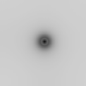
Figure 1: $\theta(\mathbf{x},t)$ near a 2D vortex.

Figure 2: $\rho(\mathbf{x},t)$ near a 2D vortex.

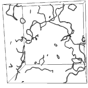
Figure 3: Plot of the low density region $\rho(\mathbf{x},t)$ below a certain threshold in a freely decay simulation.

The vortex core size is of the order of $\xi$ because, by definition, the healing length measures the size of a generic order-one fluctuation on the uniform condensate solution. By measuring circulation it is possible to distinguish between clockwise and anti-clockwise vortices. Note another important difference from the classical fluids arising from the presence of the quantum stress: vortices with the opposite sign can approach each other and annihilate.

In 3D, the vortices are more complicated objects consisting of continuous lines or loops with different topologies. These structures can oscillate producing Kelvin waves [14], be transported by the fluid or induce a fluid motion, and reconnect [8, 15]. The vortex energy is proportional, in the leading order, to its length and it can be transferred to the fluid via sound waves [16]. Examples of all these vortex motions is shown in Fig. 3: here we plot a snapshot of low density regions, associated with the vortex cores, obtained in a numerical computation of the GPE in a periodic cubic box with twelve vortices as initial condition [17].

2.2 Quantum Turbulence

Vortex-vortex dynamics (collective dynamics of vortex bundles, reconnections of vortex lines), vortex-sound (radiation and scattering of sound by vortices) and sound-sound interactions (acoustic wave turbulence) and the dynamics of the vortex itself (Kelvin waves, vortex rings) represent the ingredients of quantum turbulence (QT). When forced at the scales larger than the mean inter-vortex separation $\ell\gg\xi$, QT cascade starts as the classical Richardson cascade characteristic of Navier-Stokes turbulence until it reaches the scale $\ell$. At scales $\leq\ell$ the discreteness of the quantized vortex field becomes essential, and the further cascade to lower scales is very different than the one in the classical fluids with continuous vorticity [18, 19, 20]. After some reconnections and other crossover processes near the transitional scale $\ell$ [21, 22], the energy cascade is be carried to the scales $\leq\ell$ by Kelvin wave cascade until, at a very low scale, it is radiated into sound [18, 19, 20, 23, 24, 25, 26, 27].

In the recent years, GPE has become a popular model for studying QT by using numerical simulations [10, 9, 11, 12, 28, 29]. The pioneering paper of Nore et al. [10] showed similarities between the 3D GPE and the classical Navier-Stokes turbulence, including observations of the famous Kolmogorov $5/3$-spectrum. This spectrum was observed for scales $>\ell$ (with $\ell>\xi$), which agrees with the view that at this scales the discreteness of the vortex lines is inessential, and the turbulence picture is basically classical Kolmogorov. However, in several follow-up works [11, 12, 28] the $5/3$-spectrum was reported to extend to the smaller scales, between $\ell$ and $\xi$, where the classical Kolmogorov picture is not expected to be valid theoretically. Later in our paper we will comment on this apparent paradox.

Numerical quantities usually measured in QT can be defined in the fluid dynamic framework. Namely, the total energy is divided into kinetic, quantum and internal energy of the system as follows [10],

$$H=E_{kin}(t)+E_{qu}(t)+E_{int}(t),$$ (8)

where $E_{kin}(t)=\frac{1}{2}\int\left(\sqrt{\rho}\mathbf{v}\right)^{2}d\mathbf{x}$ is the kinetic energy , $E_{qu}(t)=\frac{1}{2}\int\left(2\nabla\sqrt{\rho}\right)^{2}d\mathbf{x}$ is the quantum energy and $E_{int}(t)=\frac{1}{2}\int\rho^{2}d\mathbf{x}=H_{nl}(t)$ the internal energy. Moreover, the quantity in the integrand of the kinetic energy is usually divided, using the Helmholtz’s theorem, into a solenoidal (incompressible) and an irrotational (compressible) vector fields,

$$\sqrt{\rho}\mathbf{v}=(\sqrt{\rho}\mathbf{v})^{i}+(\sqrt{\rho}\mathbf{v})^{c}.$$ (9)

The incompressible part, satisfying $\nabla\cdot(\sqrt{\rho}\mathbf{v})^{i}=0$, is associated to the vortex dynamics; the compressible part, which satisfies $\nabla\times(\sqrt{\rho}\mathbf{v})^{c}=0$, is related to the sound waves. Note that the mentioned above results of papers [10, 11, 12, 28] for the $k^{-5/3}$ power-law behavior refer to the spectrum of the incompressible kinetic energy $E_{kin}^{i}$.

3 Forced-dissipated GPE

The aim of this research is to study the steady turbulent states in the GPE model, with particular interest in observing cascades from large scales to small ones. Therefore, in the spirit of classical turbulence, we build a sustained system by including a forcing and a dissipation terms in the GPE:

$$\imath\frac{\partial\psi(\mathbf{x},t)}{\partial t}+\nabla^{2}\psi(\mathbf{x},t)-|\psi(\mathbf{x},t)|^{2}\psi(\mathbf{x},t)=\mathcal{F}+\mathcal{D},$$ (10)

where the forcing $\mathcal{F}$ injects mass and energy, while the dissipation $\mathcal{D}$ removes them. As a consequence, the mass and the energy are no longer constants of motion. However, if a steady turbulent state is reached, the quantities $\dot{H}(t)$ and $\dot{M}(t)$ are zero. In such a steady state, the mass and the energy get transferred from the forcing to the dissipation scales, being approximately conserved while cascading though the inertial ranges (see A).

3.1 Weak wave turbulence predictions

The WWT furnishes some prediction for wave spectra in steady states. In order to introduce WWT, let us put the system into a 3D periodic box and write the equation (neglecting $\mathcal{F}$ and $\mathcal{D}$) in Fourier space:

$$\imath\frac{\partial\tilde{\psi}(\mathbf{k}_{1},t)}{\partial t}-\omega(\mathbf{k}_{1})\tilde{\psi}(\mathbf{k}_{1},t)=\sum_{\mathbf{k}_{2},\mathbf{k}_{3},\mathbf{k}_{4}\in\mathbb{Z}^{3}}\tilde{\psi}^{\ast}(\mathbf{k}_{2},t)\tilde{\psi}(\mathbf{k}_{3},t)\tilde{\psi}(\mathbf{k}_{4},t)\delta(\mathbf{k}_{1}+\mathbf{k}_{2}-\mathbf{k}_{3}-\mathbf{k}_{4}).$$ (11)

Here $\tilde{\psi}_{i}\equiv\tilde{\psi}(\mathbf{k}_{i},t)$ is the Fourier transform of ${\psi}(\mathbf{x},t)$ and $\omega(\mathbf{k})={k}^{2}$ is the dispersion relation of the system (hereafter $k=|\mathbf{k}|$). The WWT theory, taking the limits of infinite-box limit, small nonlinearity, and assuming space homogeneity and random phases and amplitudes (RPA) of the initial wave amplitudes, provides a statistical closure. The closure predicts the behavior of statistical quantities such as correlators $\langle\tilde{\psi}_{1}\tilde{\psi}_{2}...\tilde{\psi}_{n}\tilde{\psi}_{n+1}^{\ast}\tilde{\psi}_{n+2}^{\ast}...\tilde{\psi}_{n+m}^{\ast}\rangle$, where the average is performed over the random initial data. In this framework the simplest non-trivial correlator is the second order one,

$$\langle\hat{\psi}_{i}^{\ast}\hat{\psi}_{j}\rangle=\langle|\hat{\psi}_{i}||\hat{\psi}_{j}|e^{\imath\left(\theta_{i}-\theta_{j}\right)}\rangle=n_{i}\delta(\mathbf{k}_{i}-\mathbf{k}_{j}),$$ (12)

where the quantity $n_{i}\equiv n(\mathbf{k}_{i},t)$ is called wave-action spectrum. The RPA assumption allows one to close the system by the Wick decomposition, a mechanism which splits the higher order correlators as sums of products of second order correlators [30, 31, 32]. This procedure, when applied to the GPE model, leads to the following four-wave kinetic equation for the evolution of the wave-action spectrum [33],

$$\frac{\partial n_{1}}{\partial t} = 4\pi\int n_{1}n_{2}n_{3}n_{4}\left(\frac{1}{n_{1}}+\frac{1}{n_{2}}-\frac{1}{n_{3}}-\frac{1}{n_{4}}\right)$$ (13)

$$\times\delta(\mathbf{k}_{1}+\mathbf{k}_{2}-\mathbf{k}_{3}-\mathbf{k}_{4})\delta(\omega_{1}+\omega_{2}-\omega_{3}-\omega_{4})d\mathbf{k}_{234},$$

where $d\mathbf{k}_{234}\equiv d\mathbf{k}_{2}d\mathbf{k}_{3}d\mathbf{k}_{4}$.

This is an integro-differential equation which models “wave collisions”, in analogy with Boltzmann kinetic equation for the particle collisions. Physically, it says that for times much longer that the fast wave periods $T_{i}=2\pi/\omega_{i}$, the wave amplitudes $\tilde{\psi}_{i}$ are effectively coupled only if they satisfy the following resonant conditions,

$$\begin{split}&\mathbf{k}_{1}+\mathbf{k}_{2}=\mathbf{k}_{3}+\mathbf{k}_{4}\\ &\omega_{1}+\omega_{2}=\omega_{3}+\omega_{4}.\end{split}$$ (14)

Equation (13) has the following invariants, $M=\int n(\mathbf{k},t)d\mathbf{k}$, ${\bf P}=\int\mathbf{k}n(\mathbf{k},t)d\mathbf{k}$, and $E=\int\omega(\mathbf{k})n(\mathbf{k},t)d\mathbf{k}$ that are respectively the total number of particles (or the mass), the momentum and the energy. Moreover, the dynamics described by the kinetic equation is irreversible in time and an entropy measure can be defined. Three trivial functions that cancel the integrand in (13) are $n_{k}^{(1)}=A$, $n_{k}^{(2)}=(\mathbf{B}\cdot\mathbf{k})^{-1}$ and $n_{k}^{(3)}=Ck^{-2}$ with $A,\mathbf{B},$ and $C$ constants. By combining these solutions, the general thermodynamic solution takes the form:

$$n_{k}^{(RJ)}=\frac{T}{\mu+(\mathbf{u}\cdot\mathbf{k})+k^{2}},$$ (15)

where $\mu$ is a chemical potential constant, $\mathbf{u}$ is a constant macroscopic velocity and $T$ is a temperature of the system. In an isotropic field, the macroscopic velocity is zero and the relation (15) assumes the form known in literature as Rayleigh-Jeans (RJ) thermodynamic equilibrium distribution. As the distribution is not convergent for large $k$’s, the temperature and the chemical potential can be evaluated based on the known mass and energy of the system only by introducing an ultraviolet cutoff, as proposed in [34].

In presence of an external forcing and damping, besides the RJ distribution, two other steady solutions may exist, namely the KZ spectra discussed in the introduction. These solutions have the form of a power-law $n_{k}=ck^{-\alpha}$, where $c$ is a dimensional constant. They can be obtained analytically by applying a change of integration variables known as the Zakharov transformation [3], or by a dimensional analysis [35]. The value of the exponent $\alpha$ depends on the particular wave model. KZ solutions correspond to constant fluxes of positive conserved quantities in the scale space (turbulent cascades).

The GPE model has two positive invariants, the mass $M$ and the energy $E$. It can be shown (see A) that energy has a direct cascade, i.e. from large to small scales, while the mass cascade is inverse, from small to large scales. The corresponding KZ exponents are respectively $\alpha_{E}=3$ and $\alpha_{M}=7/3$. Hereafter in this work, we present results in terms of the one-dimensional spectrum $n_{1D}(k)$, obtained from $n(k)$ by integrating out the angular variables, i.e. $n_{1D}(k)=4\pi k^{2}n_{k}$. In this notation the KZ solutions are

$$\begin{split}&n_{1D}^{(E)}(k)=4\pi c^{(E)}k^{-1}\\ &n_{1D}^{(M)}(k)=4\pi c^{(M)}k^{-1/3}.\end{split}$$ (16)

These solutions represent respectively constant fluxes of $M$ and $E$ and, therefore, they are sustained by an external forcing and a dissipation. Even tough the KZ spectra are found for infinite inertial ranges, they are expected in finite systems provided the scales of $\mathcal{F}$ and $\mathcal{D}$ are widely separated in Fourier space and provided the interactions of the wave modes are local. The locality of the KZ solutions (16) is checked in B: the energy cascade turns out to be marginally nonlocal and its locality is restored by a logarithmic correction, while the inverse particle cascade is local.

3.2 Transition to three-wave interactions

Equation (13) describes a four-wave interaction process which is responsible for the direct and the inverse cascades. When the inverse cascade is not damped at low $k$’s, it leads to accumulation of particles at these scales which can alter the four-wave dynamics. Respectively, the zero-mode $n_{\mathbf{k}=0}(t)$ (related to the uniform part of the field $\psi$ in physical space) will grow, which can be interpreted as a Bose-Einstein condensation process. When the condensate fraction becomes large, the kinetic equation (13) ceases to be valid. Suppose that a large fraction of the wave-action is present at the zero-mode, thereby $\psi(\mathbf{x},t)=c(t)+\epsilon\phi(\mathbf{x},t)$, where $\phi$ represents small fluctuations ($\epsilon\ll 1$). By substituting this ansatz into GPE (1), we find, at the order $\epsilon^{0}$, the evolution equation for the condensate fraction,

$$\imath\frac{\partial c}{\partial t}-|c|^{2}c=0.$$ (17)

Its solution is $c(t)=c_{0}e^{-\imath c_{0}^{2}t}$, where $c_{0}$ is a real positive constant. Thus, the condensate amplitude rotates in the complex plane with an angular velocity proportional to its square modulus. In the next order in $\epsilon$, we obtain a linear equation for the fluctuations on the condensate background:

$$\imath\frac{\partial\phi}{\partial t}(\mathbf{x},t)+\nabla^{2}\phi(\mathbf{x},t)-2c_{0}^{2}\phi(\mathbf{x},t)+c_{0}e^{-2\imath c_{0}^{2}t}\phi^{\ast}(\mathbf{x},t)=0.$$ (18)

Diagonalizing the linear dynamics in Fourier space, one can show that the linear wave modes oscillate at the Bogoliubov frequency [33, 36],

$$\omega(\mathbf{k})=\pm{k}\sqrt{{k}^{2}+2c_{0}^{2}}.$$ (19)

In the limit of small $k$’s or strong condensate fraction $c_{0}$, when $k^{2}\ll c_{0}^{2}$, the fluctuations are acoustic waves with the speed of sound $\omega/k\approx\sqrt{2c_{0}^{2}}$.

In the next order in $\epsilon$, when weak nonlinearity is taken into account for the fluctuations, it is possible to use the WWT theory and derive a kinetic equation describing three-wave interactions of the Bogoliubov sound [33, 36]:

$$\frac{\partial n_{1}}{\partial t}=\int(R_{231}-R_{123}-R_{312})d\mathbf{k}_{12},$$ (20)

where

$$R_{123}=2\pi|V_{123}|^{2}\delta(\mathbf{k}_{1}-\mathbf{k}_{2}-\mathbf{k}_{3})\delta(\omega_{1}-\omega_{2}-\omega_{3})(n_{2}n_{3}-n_{1}n_{2}-n_{1}n_{3})$$ (21)

and the analytical form of the scattering matrix $V_{123}$ is given in [36]. Equation (20) describes three-wave interactions $1\leftrightarrows 2$ which conserve only the energy and not the mass. Thus, only the energy cascade KZ solution is relevant to this regime. For the large-scale (strong condensate) limit $k^{2}\ll c_{0}^{2}$, the direct cascade KZ spectrum takes the form $E_{1D}(k)\sim k^{-3/2}$ predicted by Zakahrov and Sagdeev for the 3D acoustic WWT [37]. Because most of the wave-action in this case is in the condensate, the 1D energy spectrum is $E_{1D}^{(E)}(k)\sim c_{0}^{2}n_{1D}^{(E)}(k)$ [36]. Therefore, the wave-action spectrum for the energy cascade in the acoustic regime is

$$n_{1D}^{(E)}(k)\sim k^{-3/2}.$$ (22)

3.3 Critical balance conjecture

In some physical situations, wave turbulence fails to be weak, and the wave spectrum saturates at a critical shape such that the linear term is of the same size as the nonlinear term for each mode ${\bf k}$. Such a critical balance appears to be typical for a wide range of physical systems, ranging from Magneto-Hydrodynamic turbulence [38], to the rotating and stratified geophysical systems [39]. The most famous example is the Phillips spectrum of the gravity water waves [40, 41], in which case the saturation at the critical value occurs due to wave breaking.

In the GPE model, similar situation may occur when an equivalent of wave breaking process is active in the system. Namely, we will see that when the low-${\bf k}$ range is over-dissipated by strong hypo-viscosity (RUN 3), the inverse particle cascade tends to accumulate at low ${\bf k}$’s (infrared bottleneck) until a critical balance is reached and the spectrum is saturated. Indeed, for the inverse cascade to exist the wave turbulence must be weak, because only then the Fjørtoft argument works (see C). However, when the linear and the nonlinear terms, locally in Fourier space, are of the same order, the inverse cascade stops and so does the infrared bottleneck accumulation. This is precisely the mechanism of reaching the critical balance condition in this case.

Now we present an estimate for the critical balance spectrum in the GPE model. Equating the linear and the nonlinear terms in Fourier space gives

$$\begin{array}[]{rcl}k^{2}|\tilde{\psi}_{k}|&\sim&|\tilde{\psi}_{k}|^{3}k^{6}\\ \Rightarrow\;k^{-4}&\sim&|\tilde{\psi}_{k}|^{2}.\end{array}$$ (23)

Note that we have replaced each $d\mathbf{k}$ integration by $k^{3}$ thereby assuming that only the wave amplitudes with similar $k$’s are correlated in Fourier space. Thus, for the 1D wave-action spectrum in the critical balance regime, we have

$$n_{1D}^{(CB)}(k)\sim k^{-2}.$$ (24)

4 The numerical experiments

As we want to understand the basic properties of the GPE turbulence, we choose to deal with the simplest configuration: triple periodic boundary condition and uniform mesh grid. With this choice we can use the discrete Fourier transforms which are numerically fast [42, 43]. In our numerics the complex wave field $\psi$ is a double precision variable defined in space over $256^{3}$ points. The simulation box has side $L=256$ and so the Fourier space width is $L_{k}=2\pi$ with resolution $\Delta k=2\pi/256$. Without considering for the moment the forcing and the dissipation terms, the GPE model (1) can be written in the physical space as a sum of a linear operator $\mathcal{L}$ and a nonlinear one $\mathcal{G}$

$$\imath\frac{\partial\psi}{\partial t}=\mathcal{L}\psi+\mathcal{G}\psi,$$ (25)

where $\mathcal{L}=-\nabla^{2}$ and $\mathcal{G}=|\psi|^{2}$. We then use a split step method to solve separately the contributions of the two operators in time. This choice is very useful because the linear operator has the exact solution in Fourier space, $\tilde{\psi}(\mathbf{k},t+\Delta t)=\tilde{\psi}(\mathbf{k},t)e^{-\imath|\mathbf{k}|^{2}\Delta t}$, while the nonlinear one, due to the conservation of the mass in the system, has the analytic solution $\psi(\mathbf{x},t+\Delta t)=\psi(\mathbf{x},t)e^{-i|\psi(\mathbf{x},t)|^{2}\Delta t}$ in the physical space. At each time step $\Delta t$, we first evaluate the linear part in Fourier space and then use this temporary solution to solve the nonlinear part in the physical space. With this choice, the numerical error in the algorithm is only due to the time-splitting [44]. The time step is always $\Delta t=0.5$, chosen to be of the order of the shortest linear time $2\pi/\omega_{max}$.

Concerning the forcing and the dissipation, it appears convenient to control $\mathcal{F}$ and $\mathcal{D}$ directly in Fourier space to gain a wide inertial range. The forcing term acts to inject mass and energy in the system. In all simulations, $\mathcal{F}$ modifies the first (linear) calculation half-step as follows,

$$\tilde{\psi}(\mathbf{k},t+\Delta t)=\left\{\begin{array}[]{ll}\tilde{\psi}(\mathbf{k},t)e^{-\imath|\mathbf{k}|^{2}\Delta t}+Af_{0}e^{\imath\varphi(\mathbf{k},t)},&k_{\min}\leq|\mathbf{k}|\leq k_{\max}\\ \tilde{\psi}(\mathbf{k},t)e^{-\imath|\mathbf{k}|^{2}\Delta t},&|\mathbf{k}|<k_{\min}\cup|\mathbf{k}|>k_{\max},\end{array}\right.$$ (26)

where $A\simeq 1.62\times 10^{-3}$. Thus the pumping add mass and energy in the ring region $k_{\min}\leq|\mathbf{k}|\leq k_{\max}$ with the function $\varphi(\mathbf{k},t)$ uniformly distributed in $[0,2\pi)$ and statistically independent at each $\bf k$-space and each time step. We choose the forcing at relatively large scales, with $k_{\min}=9\Delta k$ and $k_{\max}=10\Delta k$. A dissipation at high wave numbers is added to halt the direct cascade and to prevent termalization effects. We find that an hyper-viscous term $\mathcal{D}_{h}=\imath\nu_{h}(\nabla^{2})^{8}\psi(\mathbf{x},t)$, where $\nu_{h}=2\times 10^{-6}$, is effective in absorbing the high-$k$ spectrum and in preventing the aliasing and the bottleneck effects. This term is also added to the linear operator to evaluate it efficiently in Fourier space. Finally, different types of dissipations at the large scales can be chosen. In this manuscript we report three different setups, briefly summarized in Table 1, whose results are discussed in the following.

cases	forcing	dissipation at low $k$’s	dissipation at high $k$’s
RUN 1	$f_{0}=0.1$	none	$\mathcal{D}_{h}=\imath\nu_{h}(\nabla^{2})^{8}\psi(\mathbf{x},t)$
RUN 2	$f_{0}=0.1$	$\hat{\mathcal{D}}_{l}=\imath\theta(k^{\star}-|\mathbf{k}|)\tilde{\psi}(\mathbf{k},t)$	$\mathcal{D}_{h}=\imath\nu_{h}(\nabla^{2})^{8}\psi(\mathbf{x},t)$
RUN 3	various	$\mathcal{D}_{l}=\imath\nu_{l}(\nabla^{-2})^{8}\psi(\mathbf{x},t)$	$\mathcal{D}_{h}=\imath\nu_{h}(\nabla^{2})^{8}\psi(\mathbf{x},t)$

Table 1: Summary of the different numerical simulations performed. Here the hat operator $\hat{\cdot}$ stands for the Fourier-space operator, $\nu_{h}=2\times 10^{-6}$, $\nu_{l}=1\times 10^{-18}$, $\mu=1\times 10{-4}$, $k^{\star}=9\Delta k$ and the forcing is defined in (26).

4.1 RUN 1 - free condensate growth

Here, we study the evolution of the GPE system, initially empty, without any dissipation at low $\mathbf{k}$’s. At every time step, the forcing term inputs mass $\Delta M(t)$ and energy $\Delta E(t)$, so that $M$ and $E$ start to grow. Even if the forcing is acting at a particular wave-number range, the nonlinear interactions cause mass and energy transfers in Fourier space. We have chosen the forcing coefficient $f_{0}$ such that the transfers become efficient for the time step considered, namely it chosen to be sufficiently big to prevent sandpile effects characteristic to mesoscopic turbulence [45, 46]. One can see in Fig. 4 that at early stages of the simulation the wave-action spectrum $n_{1D}(k,t)$ evolves and spreads over the wave-numbers space: the energy and the particles undergo a direct and an inverse cascades respectively.

Figure 4: Wave-action spectrum $n_{1D}(k,t)$ during initial stages of simulation. The time unit $\tau$ refers to the linear time of the forcing scale.

After an initial transient time, the linear energy density $\mathcal{E}_{lin}(t)$ stops to grow, as clearly visible in Fig. 5. Linear energy weights at the high wave number part of the spectrum and this saturation is an evidence that its transfer to the small scales is now absorbed by the hyper-viscosity. On the contrary, as no dissipation is present at the large scales, the inverse particle cascade is not arrested and the nonlinear energy density $\mathcal{E}_{nl}(t)$ continues to increase.

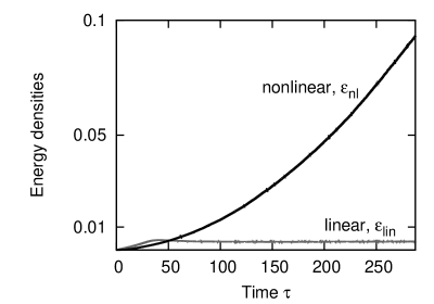
Figure 5: Linear $\mathcal{E}_{lin}(t)$ and nonlinear $\mathcal{E}_{nl}(t)$ energy densities during the RUN 1.

4.1.1 Spectra

In Fig. 6 we present the 1D wave-action spectrum at two different stages after the stabilization of the linear energy. The spectrum plotted with dashed line is taken at early stages, when the linear and the nonlinear energy densities are comparable: at this point there is a good agreement with the WWT $k^{-1}$ prediction, which is also plotted.

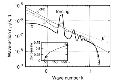
Figure 6: Wave-action spectrum $n_{1D}(k,t)$ at two different stages of RUN 1. The four-wave and the three-wave WWT predictions are also indicated by the lines with slopes $-1$ and $-3/2$ respectively. Inset: evolution of the condensate component $c_{0}(t)$.

The condensate component $c_{0}(t)$ continues to increase during the simulation, as shown in inset to Fig. 6, and a well defined series of peaks appears in the wave-action spectrum at the final stage (continuous line). Such behavior is a clear sign of three-wave interactions, as reported in [47]. Note that the late stage spectrum is consistent with the three-wave Zakharov-Sagdeev WWT prediction $k^{-3/2}$. The acoustic three-wave regime is also confirmed by evaluating the dispersion relation by measuring the wavenumber-frequency Fourier transform. The result, presented in Fig. 7, shows the presence of two branches (one for the Bogoliubov mode and another for its conjugate) shifted by the condensate velocity oscillation $c_{0}^{2}$, in excellent agreement with the corresponding Bogoliubov dispersion (19).

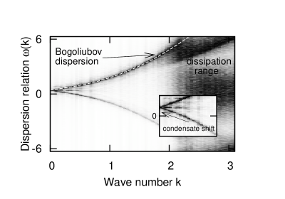
Figure 7: Dispersion relation at the final stage of RUN 1, when the condensate fraction is strong. The white dashed line is the Bogoliubov dispersion (only the upper branch). Inset: a zoom on the small $k$’s zone to appreciate the shift due to the presence of the condensate.

The observed evolution of the spectrum can be summarized as follows. (a) At initial times the condensate wave amplitude $\tilde{\psi}_{\mathbf{k}=0}(t)$ is of the same order as the amplitude of other modes and the dynamics is well described by the four-wave WWT regime. (b) As the inverse cascade is not halted, mass accumulates at low $\mathbf{k}$’s and strong turbulence takes place in this transition. (c) Finally when the zero-mode becomes dominant over the fluctuations the wave turbulence is again weak and well described by the three-wave WWT.

4.1.2 Condensation and density PDF

To access further information about the statistics of the transition from the four-wave to the three-wave regime during the condensation process, in Fig. 8 we show the probability density function (PDF) of the density field $\rho$ at initial and final stages.

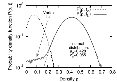
Figure 8: Probability density function of the density field $\rho$ at different time: early stages ($t_{a}$) and final stage ($t_{b}$) in RUN 1. A normal distribution with mean $\mu$ and standard deviation $\sigma$ are indicated.

At early stages the density remains small with a lot of low density regions present, which indicates presence of numerous “ghost” (weakly nonlinear) vortices. In fact, in the ideal four-wave WWT dynamics, the wave field would be nearly Gaussian, and the respective density $\rho$ would have an exponential (Rayleigh) PDF, which would be a straight line (with a negative slope) in Fig. 8. We see a significant deviation from the Rayleigh behavior, which means that even at an early stage (at time $t_{a}$ when the four-wave KZ spectrum is reported) the statistics already differed from the Gaussian. The development of a maximum on the PDF of $\rho$ is a signature of the emerging condensate. As the inverse cascade is not halted the condensate density keeps growing in time. At final stages (at time $t_{b}$ when the three-wave KZ spectrum is reported) the density field shows a normal distribution behavior in the core of the PDF with a tail remaining at low density regions corresponding to vortices (which are now strongly nonlinear). Note that the mean value of $\rho$ at this time (0.428) is much greater than the standard deviation (0.055) which means that the condensate density is much stronger that the Boboliubov fluctuations about the mean density. This is a clear sign of the three-wave WWT.

4.1.3 Vortices and velocity PDF

Now let us focus on the vortex component represented by the low-$\rho$ PDF tail at $t=t_{b}$. By plotting the iso-surfaces with small density threshold ($\rho_{thr}=0.1$) only one quantum vortex is found in the computational box. We plot in Fig. 9 its evolution, showing only a part of the total box. The vortex has a ring shape and it propagates in the direction of the ring axis. The vortex core radius is consistent with the healing length estimate $\xi\simeq 1.5=1.5\Delta x$. Propagating Kelvin waves can be observed on the vortex line. We will argue below that these waves are crucial for understanding the $5/3$-spectrum of the incompressible kinetic energy.

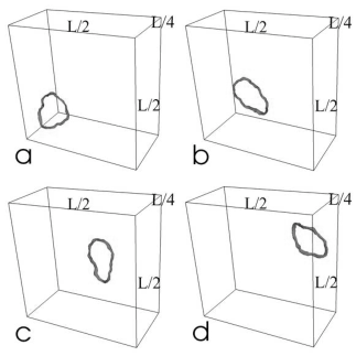
Figure 9: Snapshots of iso-surfaces of low density region with threshold $\rho_{thr}=0.1$ (the mean density is $\langle\rho\rangle\simeq 0.43$). The box is $1/2\times 1/2\times 1/4$ the computational domain. The frames are taken approximately every $3\tau$.

In Fig. 10 we plot the PDF of the single velocity components (the data are normalized in order to compare different distributions).

Figure 10: Probability density function of the single velocity components at the final stage in RUN 1. Inset: zoom on the positive tail of the distribution in log-log coordinates.

The velocity PDF appears to have a dominant Gaussian core, which is consistent with the three-wave WWT. In addition, the velocity PDF power-law tail with exponent $-3$ is another signature of the thin vortex lines, whose velocity field falls off inversely proportional to the distance from the line at short distances. Such power-law velocity PDF’s where observed in superfluid turbulence experimentally [48] and numerically [29] and interpreted as an evidence of quantum vortices.

4.1.4 Incompressible energy spectrum

Spectra of the compressible and the incompressible kinetic energy at late time ($t=t_{b}$) are presented in Fig. 11.

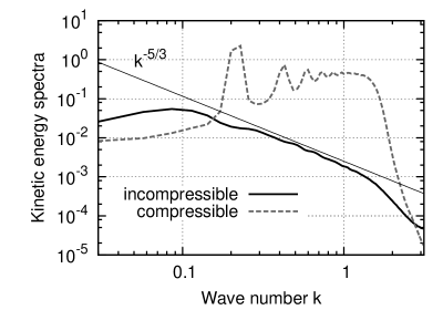
Figure 11: Compressible and incompressible kinetic energy spectra measured at final stage of simulation in RUN 1. A $k^{-5/3}$ showin classical Kolmogorov prediction is also plotted.

The compressible part is dominant and has the same features as the ones already discussed for the wave-action spectrum: it shows the peaks (harmonics of the forcing scale) and it follows the Zakharov-Sagdeev spectrum (with exponent $-3/2+2=1/2$). The incompressible spectrum formally coincides with the classical Kolmogorov $5/3$-law. But we have seen in Fig. 9 that only one quantized vortex ring remains in the system at this time, so it is impossible for the Kolmogorov theory, developed for the continuous classical vorticity fields, to be relevant in this case. Resolution to this paradox is suggested in [49]. In short, the $-5/3$ slope is produced by an energy cascade carried by Kelvin waves (seen in Fig. 9). It turns out [27] that the Kelvin wave energy spectrum also has exponent $-5/3$ and the coincidence with the Kolmogorov exponent is purely coincidental (the Kelvin-wave and the Kolmogorov spectra have different pre-factors).

4.2 RUN 2 - friction at large scales

In the previous run no steady turbulent state has been reached because of the presence of the inverse cascade. To stay in the four-wave weak turbulence regime and to avoid the condensate growth, an effective friction term at large scales will now be added. This term is written directly in Fourier space and results in

$$\hat{\mathcal{D}}_{l}=\imath\mu\theta(k^{\star}-|\mathbf{k}|)\tilde{\psi},$$ (27)

where $\theta$ is the Heaviside step function, $k^{\star}=9\Delta k$ is the lowest forced wave-number and $\mu=1\times 10^{-4}$ is a friction coefficient. This coefficient is optimally chosen to stop the inverse cascade without altering the direct energy cascade. With this choice both the nonlinear and the linear energy densities reach a constant value during the simulation, as plotted in Fig. 12.

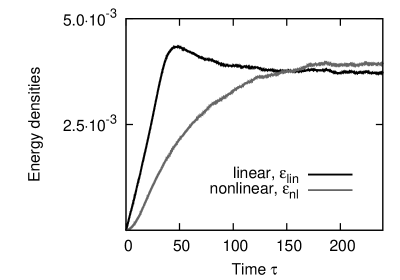
Figure 12: Linear $\mathcal{E}_{lin}(t)$ and nonlinear $\mathcal{E}_{nl}(t)$ energy density evolution in the presence of large scale friction (RUN 2).

The final stage wave-action spectrum, presented in Fig. 13, agrees with the $k^{-1}$ four-wave WWT prediction. The condensate growth, shown in the inset, is halted by the friction. Agreement with the four-wave WWT may seem surprising because, according to Fig. 12, the nonlinear energy exceeds the linear one. Our explanation is that the nonlinear energy mostly resides in the condensate and forcing scales, whereas in the direct cascade range the modes are weakly nonlinear.

Figure 13: Wave-action spectrum $n_{1D}(k,t)$ at final stage of simulation in the presence of friction. The WWT four-wave prediction $k^{-1}$ is shown by the straight line. The inset shows the condensate evolution $c_{0}(t)$.

We now turn our attention to the statistically steady state distributions in the physical space. The PDF of the density field $\rho$, not showed here, looks similar to early stage distribution presented in Fig. 8. Here the average density is $\langle\rho\rangle\simeq 8.31\cdot 10^{-2}$, which corresponds to healing length $\xi\simeq 3.5\Delta x$. The low density regions in the computational box are plotted in Fig. 14.

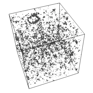
Figure 14: Low density region of the density field, threshold $\rho_{thr}=0.015$, in presence of friction (RUN 2).

A big fuzzy ring structure is present in the top of the figure. It is probably a single ring with large fluctuations, which create secondary small vortex loops near the main vortex. Besides this ring, other uniform bubble-like low density regions are present in the box. These are small scale ghost vortices which are weakly nonlinear and short-lived (their typical size is close to the resolution scale). Thus we see that even though the wave field is mostly random, the coherent vortex structures are also seen in this regime.

The system in the fluid dynamics framework presents quite unexpected results, still remaining to be explained. The PDFs of the velocity components are plotted in Fig. 15.

Figure 15: Probability density function of velocity components in the presence of friction (RUN 2). Inset: zoom in log, log scale of the positive PDFs branch.

The PDF is isotropic and Gaussian in the core, but it has a power-law tail $\sim v_{i}^{-5.3}$. We still do not have a theoretical explication for this exponent, although the power-law PDF tail with a different exponent (-1) was previously predicted for WWT in [30]. The compressible and the incompressible kinetic energy spectra are presented in Fig. 16.

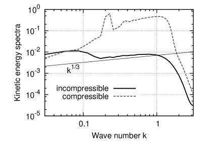
Figure 16: Compressible and incompressible kinetic energy spectra in a steady state with friction (RUN 2).

The compressible spectrum does not show peaks (as in RUN 1) indicating that this turbulence is not acoustic. The incompressible spectrum shows a power-law behavior with exponent close to $1/3$. Again, no theoretical explanation could be proposed.

4.3 RUN 3 - hypo-viscosity dissipation

One can devise to stop the inverse cascade with a different type of dissipation at low $k$’s. For this, let us now choose a hypo-viscosity of the form

$$\mathcal{D}_{l}=\imath(\nabla^{-2})^{8}\psi(\mathbf{x},t).$$ (28)

As this operator is singular in $\mathbf{k}=0$, we will separately remove, at each time step, the zero-mode in Fourier space. This choice still allows to reach steady turbulent states, but unexpectedly leads to different results with respect to RUN 2. In Fig. 17 we present various steady state spectra evaluated with different levels of the forcing $f_{0}$.

Figure 17: Wave-action spectra $n_{1D}(k,t)$ at the final stage of the simulation in the presence of hypo-viscosity (RUN 3) for different forcing coefficients: $f_{0}=0.05$ (A), $f_{0}=0.1$ (B), $f_{0}=0.5$ (C), $f_{0}=1.0$ (D), $f_{0}=2$ (E), $f_{0}=3$ (F). The $k^{-1}$ WWT and $k^{-2}$ CB predictions are also shown.

What emerges clearly is that the spectra still have a power-law behavior in the inertial range, but it does not follow the WWT four-wave prediction $k^{-1}$. Instead, we see the $k^{-2}$ critical balance prediction for the wide range of the forcing amplitudes.

Our interpretation is the following. The hypo-viscosity causes an infrared bottleneck that alters the dynamics at the scales near the forcing: there the linear and the nonlinear energies become comparable. At this point the Fjørtoft argument can no longer apply and the critical balance condition propagates into all the inertial range causing the observed $k^{-2}$ spectra. This suggestion is corroborated by the measurement of the ratio between nonlinear and linear energies $\eta={H_{nl}}/{H_{lin}}$ evaluated for various forcing coefficients $f_{0}$ illustrated in Fig. 18.

Figure 18: Energy ratio $\eta=H_{nl}/H_{lin}$ with respect to different forcing coefficients $f_{0}$ in the presence of hypo-viscosity (RUN 3). For informations about labels see caption in Fig. 17.

From these results it is clear that, for a wide range of the forcing coefficients (almost two orders of magnitude), the energy ratio $\eta$ remains always order one.

As in the previous runs, we look at the density field in the physical space to visualize vortices and other turbulent structures. For this we choose the case (D) when $f_{0}=1.0$ (all other cases look similar). Again, the PDF of the density is similar to the early stage PDF in Fig. 8, and this is natural because there is no condensate in the present system. The mean density is $\langle\rho\rangle\simeq 4.31\cdot 10^{-1}$ and so $\xi\simeq 1.5\Delta x$. In Fig. 19 we show the low density regions in the physical space with a threshold $\rho_{thr}=0.05$. This figure is qualitatively different from the previous ones (Fig. 9 and Fig. 14). Now very thin vortex structures fill completely the computational box and form a “vortex tangle”.

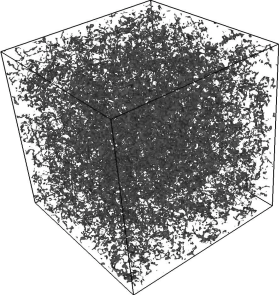
Figure 19: Low density regions with threshold of $\rho_{thr}=0.05$ are plotted at the final stage with the presence of hypo-viscosity with $f_{0}=1.0$ (RUN 3).

The one point PDF’s of the single velocity components are plotted in Fig. 20.

Figure 20: PDF of single velocity components in the presence of hypo-viscosity with $f_{0}=1.0$ (RUN 3). Inset: zoom of the positive branch of the PDF in log-log coordinates.

The PDF’s, which show isotropy, are strongly non-Gaussian: the power-law behavior of $v^{-3}$ is observed. This result is interesting because similar behavior was observed experimentally in [48] and numerically in [29] and explained by presence of thin quantized vortex lines. We emphasize the $v^{-3}$ PDF behavior is dominant and not present just in the tail as in the RUN 1. This is because we have much more strong vortex lines in the RUN 3 than in the RUN 1. Indeed, as the condensate fraction is removed by this type of dissipation, it is thus natural to think that the vortices fill the system at all scales and highly influence the velocity field. These vortex lines undergo frequent reconnections resulting in a sound emission. The incompressible kinetic energy spectra, for all the forcing amplitudes, are illustrated in Fig. 21.

Figure 21: Incompressible kinetic energy spectra for different forcing amplitude $f_{0}$ in presence of hypo-viscosity (RUN 3). For information about the labels see caption in Fig. 17.

No evidence of $-5/3$ law is found in this (critical balanced) regime. All spectra have a power-law behavior in the inertial range with exponent near $-1$. A theoretical explanation of this exponent is still lacking.

5 Conclusions

In this paper, we have analyzed the turbulent states in the forced-dissipated 3D GPE model by using the direct numerical simulations. Introduction of the forcing and the damping is aimed at achieving statistically stationary turbulent cascades. We have focused our attention on the direct energy cascade by introducing a pumping term at relatively large scales and by using hyper-viscosity at small scales. We have studied three regimes with different dampings at the scales larger than the forcing scale: no dissipation (RUN 1), a friction (RUN 2) and a hypo-viscosity (RUN 3).

RUN 1 is performed without any dissipation at large scales and so the inverse cascade, predicted by the WWT theory, causes condensation at the $k=0$ mode. This alters the four-wave dynamics and the system, after a strongly turbulent transient, becomes dominated by weak three-wave dynamics of acoustic fluctuations on background of a strong coherent condensate. The long-time evolution in this case is characterized by the appearance of a large quantum vortex ring in the numerical box. Kelvin waves propagate on this vortex ring, which causes the incompressible kinetic energy spectrum to follow the $-5/3$ law. We argue that the classical turbulence picture developed for the continuous vorticity fields is inapplicable; the fact that the Kelvin wave turbulence has the same spectrum as the classical Kolmogorov spectrum is coincidental, as it arises from completely different physical processes [27, 49]. The vortex ring in this regime coexists with the random acoustic waves engaged in the three-wave interactions. The vortex shows up as a $v^{-3}$ tail on the velocity PDF while the random waves make up the Gaussian core of this PDF.

In RUN 2 and RUN 3 we have introduced a dissipation term at large scales in order to stop the inverse cascade and to reach statistically steady states. The characteristics of these states depend strongly on the choice of the low-$k$ damping. If a friction is introduced (RUN 2), the growth of the condensate is halted and the wave-action spectrum follows the four-wave WWT prediction. A large fuzzy vortex ring surrounded by small ghost vortices appears in the final stage of the computation. If the dissipation is an hypo-viscosity (RUN 3), the final steady spectra, evaluated for a wide range of forcing coefficient, agree with the critical balance prediction. In this regime the computational box appears to be filled by a vortex tangle - a chaotic set of strongly nonlinear vortex lines. The velocity PDF exhibits, both in the core and on the tails, a power-law behavior $v^{-3}$ characteristic to such vortex lines.

In Summary, our numerical results clearly show that the turbulent state in the direct cascade range is strongly affected by the choice of damping in the inverse cascade range. Most realistic configuration for the existing BEC experiments is configuration of RUN 1. Indeed, while the hyper-viscosity can be physically understood as an evaporative cooling mechanism, no large-scale damping mechanisms have ever been proposed. On the other hand, to study the nontrivial QT states predicted by the RUN 2 and the RUN 3 of the present paper, it would be interesting to explore possibilities to damp the lowest-momentum modes in BEC experiments.

6 Acknowledgments

We thank Al Osborne and Victor L’vov for always stimulating discussions and for suggestions. We are also grateful to Guido Boffetta, Filippo De Lillo and Stefano Musacchio for precious advises on classical turbulence and numerics. We appreciate the work of FFTW developers in providing an excellent package to perform FFT algorithm.

Appendix A Signs of the fluxes

The KZ solutions carry constant fluxes of the conserved quantities over the turbulent scales. The GPE model has two conserved quantities: the mass (particles) and the energy. Here, we will find the direction of the fluxes corresponding to the KZ solutions in a very simple way, avoiding computing the flux based on a complicated relation resulting from the the kinetic equation, as it was done in [50] and [33].

Consider Fig. 22

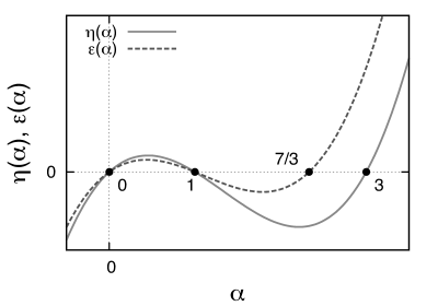
Figure 22: Qualitative direction behaviors of energy and particles fluxes with respect to the power-law exponent $\alpha$ of KZ solution $n(k)=ck^{\alpha}$.

where we qualitatively plot the flux on a generic power-law spectrum $n(k)=ck^{-\alpha}$ (which is note necessarily a steady solution) as a function of the exponent $\alpha$. For very sharp spectra, $\alpha\gg 1$, both fluxes must be positive. To see that one can think of a narrow-band spectrum: it must spread which corresponds to the positive fluxes on the negative slope side. As the fluxes are continuous functions of $\alpha$, we can determine their directions based on the zero-crossing points, i.e. the RJ and the KZ exponents. Of course, at the two thermodynamic RJ solutions, corresponding to $\alpha=0$ and $\alpha=1$, both fluxes must be zero. At the KZ solutions, only one of the fluxes turns into zero. Namely, on the energy cascade KZ, the mass flux is null and vice versa. Thus, the functions $\eta(\alpha)$ and $\epsilon(\alpha)$ qualitatively behave as shown in Fig. 22. It is then clear that the energy undergoes a direct cascade while the mass cascade inversely.

Appendix B Locality of interactions

Lets test the locality of interactions in the constant-flux states. This imply checkig that the collision integral in the kinetic equation (13) converges on the KZ spectra $n(k)=ck^{-\alpha}$. As these solutions are scale-invariant, the integral is easily written in the $\omega$ space as

$$I(\omega_{1})= \frac{c^{3}}{8\omega_{1}^{\frac{\alpha}{2}}}\int(\omega_{2}\omega_{3}\omega_{4})^{\frac{-\alpha+d-1}{2}}\left(\omega_{1}^{\frac{\alpha}{2}}+\omega_{2}^{\frac{\alpha}{2}}-\omega_{3}^{\frac{\alpha}{2}}-\omega_{4}^{\frac{\alpha}{2}}\right)$$ (29)

$$\times\delta(\omega_{1}+\omega_{2}-\omega_{3}-\omega_{4})f(\omega_{1},\omega_{2},\omega_{3},\omega_{4})d\omega_{234},$$

where term

$$f(\omega_{1},\omega_{2},\omega_{3},\omega_{4})=\frac{\min\left[\sqrt{\omega_{1}},\sqrt{\omega_{2}},\sqrt{\omega_{3}},\sqrt{\omega_{4}}\right]}{2(\omega_{1}\omega_{2}\omega_{3}\omega_{4})^{\frac{1}{2}}}$$ (30)

takes into account the 3D average of $\delta(\mathbf{k}_{1}+\mathbf{k}_{2}-\mathbf{k}_{3}-\mathbf{k}_{4})$ over the solid angles $\Omega_{1},\Omega_{2},\Omega_{3}$ and $\Omega_{4}$ , see [3, 33, 51, 52] for details. In this coordinate system the frequency $\delta$-function can be easily used, for example as $\omega_{2}=\omega_{3}+\omega_{4}-\omega_{1}$. The integral presents singularities for integration over $\omega_{3}$ at zero and infinity. Note that is the same is true for $\omega_{4}$ integration as the integral is symmetric with respect to $(3,4)\rightarrow(4,3)$. By Taylor expanding the integrand up to the leading order, one gets

$$\begin{split}&\lim_{\omega_{3}\rightarrow\infty}I(\omega_{1})\sim\int\omega_{3}^{-\frac{\alpha+2}{2}}d\omega_{3}\;\;\;\mbox{and}\\ &\lim_{\omega_{3}\rightarrow\ 0}I(\omega_{1})\sim\int\omega_{3}^{-\frac{\alpha-1}{2}}d\omega_{3}.\end{split}$$ (31)

The locality holds for $0<\alpha<3$ which is true for the inverse particles cascade ($\alpha=7/3$) but not for the direct energy cascade ($\alpha=3$). Nevertheless the divergence in the latter case is marginal and the solution can be corrected by a logarithmic factor [33].

Appendix C The Fjørtoft argument

We will present here a new version of the argument Fjørtoft argument which is formulated for the conservative systems (no forcing or dissipation). Let us introduce the mass and the energy centroids as

$$K_{M}=\frac{\int kn(k)dk}{M}$$ (32a)

$$K_{E}=\frac{\int k\mathcal{E}(k)dk}{E}=\frac{\int k^{3}n(k)dk}{E}.$$ (32b)

In the latter expression we have assumed (this is essential for the Fjørtoft argument) that the nonlinear energy is negligible with respect to linear one. In the following will use the Cauchy-Schwartz inequality

$$\int f(k)g(k)dk\leq\left(\int f^{2}(k)dk\right)^{1/2}\left(\int g^{2}(k)dk\right)^{1/2}$$ (33)

By splitting the energy integrand in two parts we get

$$E = \int k^{2}n(k)dk=\int(k^{1/2}n^{1/2})\times(k^{3/2}n^{1/2})dk$$ (34)

$$\leq \left(\int kn(k)dk\right)^{1/2}\left(\int k^{3}n(k)dk\right)^{1/2}=\sqrt{K_{M}MK_{E}E}$$

and so we have

$$K_{M}K_{E}\geq\frac{E}{M}.$$ (35)

This inequality means that if the particle centroid moves to low wave numbers (inverse cascade) the energy centroid must move to high wave numbers (direct cascade).

We now evaluate

$$K_{M}M = \int kn(k)dk=\int(kn^{1/2})\times(n^{1/2})dk$$ (36)

$$\leq \left(\int k^{2}n(k)dk\right)^{1/2}\left(\int n(k)dk\right)^{1/2}=\sqrt{ME}$$

which gives

$$K_{M}\leq\sqrt{E/M}.$$ (37)

This inequality means that the mass centroid can either stay where it is initially, or move to the large scales (inverse cascade), but it cannot cascade to the small scales.

Combining the inequalities (35) and (37), we get

$$K_{E}\geq\sqrt{E/M}.$$ (38)

This inequality means that if the energy centroid can either stay where it was initially, or move to the smaller scales (direct cascade), but it cannot cascade to the larger scales.

References

- [1] U. Frisch, Turbulence: the legacy of AN Kolmogorov, Cambridge University Press, 1995.
- [2] V. Zakharov, Weak turbulence in media with decay spectrum,, J. Appl. Mech. Tech. Phys. (4) (1965) 22–24.
- [3] V. Zakharov, V. L’vov, G. Falkovich, Kolmogorov Spectra of Turbulence 1: Wave Turbulence, Springer-Verlag, 1992.
- [4] V. Zakharov, N. Filonenko, Energy Spectrum for Stochastic Oscillations of the Surface of a Liquid, in: Soviet Physics Doklady, Vol. 11, 1967, p. 881.
- [5] S. Nazarenko, Wave Turbulence, Springer-Verlag, 2010.
- [6] C. Sulem, P. Sulem, The Nonlinear Schrödinger Equation: Self-Focusing and Wave Collapse, Springer, 1899.
- [7] F. Dalfovo, S. Giorgini, L. Pitaevskii, S. Stringari, Theory of Bose-Einstein condensation in trapped gases, Reviews of Modern Physics 71 (3) (1999) 463–512.
- [8] J. Koplik, H. Levine, Vortex reconnection in superfluid helium, Physical Review Letters 71 (9) (1993) 1375–1378.
- [9] N. Berloff, B. Svistunov, Scenario of strongly nonequilibrated Bose-Einstein condensation, Physical Review A 66 (1) (2002) 13603.
- [10] C. Nore, M. Abid, M. Brachet, Decaying Kolmogorov turbulence in a model of superflow, Physics of Fluids 9 (1997) 2644.
- [11] M. Kobayashi, M. Tsubota, Kolmogorov Spectrum of Superfluid Turbulence: Numerical Analysis of the Gross-Pitaevskii Equation with a Small-Scale Dissipation, Physical Review Letters 94 (6) (2005) 65302.
- [12] M. Kobayashi, M. Tsubota, Kolmogorov spectrum of quantum turbulence, JOURNAL-PHYSICAL SOCIETY OF JAPAN 74 (12) (2005) 3248.
-
[13]
D. Proment, S. Nazarenko, M. Onorato,
Quantum turbulence
cascades in the gross-pitaevskii model, Physical Review A (Atomic,
Molecular, and Optical Physics) 80 (5) (2009) 051603.
doi:10.1103/PhysRevA.80.051603.
URL http://link.aps.org/abstract/PRA/v80/e051603 -
[14]
E. Kozik, B. Svistunov,
Kolmogorov and
kelvin-wave cascades of superfluid turbulence at t = 0: What lies between,
Physical Review B (Condensed Matter and Materials Physics) 77 (6) (2008)
060502.
doi:10.1103/PhysRevB.77.060502.
URL http://link.aps.org/abstract/PRB/v77/e060502 -
[15]
S. Z. Alamri, A. J. Youd, C. F. Barenghi,
Reconnection of
superfluid vortex bundles, Physical Review Letters 101 (21) (2008) 215302.
doi:10.1103/PhysRevLett.101.215302.
URL http://link.aps.org/abstract/PRL/v101/e215302 - [16] M. Leadbeater, T. Winiecki, D. Samuels, C. Barenghi, C. Adams, Sound emission due to superfluid vortex reconnections, Physical Review Letters 86 (8) (2001) 1410–1413.
-
[17]
D. Proment, S. Nazarenko, M. Onorato,
Quantum vortex decay
(movie).
URL http://www.youtube.com/watch?v=uk5DpF4vnFs - [18] W. F. Vinen, J. Niemela, Journal of Low Temperature Physics 128 (2002) 167.
- [19] W. F. Vinen, Classical character of turbulence in a quantum liquid, Phys. Rev. B 61 (2) (2000) 1410–1420. doi:10.1103/PhysRevB.61.1410.
- [20] W. F. Vinen, Decay of superfluid turbulence at a very low temperature: The radiation of sound from a kelvin wave on a quantized vortex, Phys. Rev. B 64 (13) (2001) 134520. doi:10.1103/PhysRevB.64.134520.
- [21] V. L’vov, S. Nazarenko, O. Rudenko, Bottleneck crossover between classical and quantum superfluid turbulence, Phys Rev B 76 (2) (2007) 024520.
- [22] V. L’vov, S. Nazarenko, O. Rudenko, Gradual eddy-wave crossover in superfluid turbulence, Journal of Low Temperature Physics 153 (5-6) (2008) 140–161.
- [23] E. Kozik, B. Svistunov, Kelvin-wave cascade and decay of superfluid turbulence, Phys. Rev. Lett. 92 (3) (2004) 035301. doi:10.1103/PhysRevLett.92.035301.
- [24] G. Boffetta, A. Celani, D. Dezzani, J. Laurie, S. Nazarenko, Modeling Kelvin Wave Cascades in Superfluid Helium, Journal of Low Temperature Physics 156 (3-6) (2009) 193–214.
- [25] S. Nazarenko, Kelvin wave turbulence generated by vortex reconnections, JETP Letters 84 (11) (2006) 585–587.
- [26] S. Nazarenko, Differential approximation for Kelvin-wave turbulence, JETP Letters 83 (5) (2005) 198–200.
- [27] V. L’vov, S. Nazarenko, Spectrum of Kelvin-wave turbulence in superfluids, JETP Letters 91 ((8)) (2010) 464–470.
-
[28]
J. Yepez, G. Vahala, L. Vahala, M. Soe,
Superfluid turbulence
from quantum kelvin wave to classical kolmogorov cascades, Physical Review
Letters 103 (8) (2009) 084501.
doi:10.1103/PhysRevLett.103.084501.
URL http://link.aps.org/abstract/PRL/v103/e084501 - [29] A. C. White, C. F. Barenghi, N. P. Proukakis, A. J. Youd, D. H. Wacks, Nonclassical velocity statistics in a turbulent atomic bose-einstein condensate, Phys. Rev. Lett. 104 (7) (2010) 075301. doi:10.1103/PhysRevLett.104.075301.
- [30] Y. Choi, Y. Lvov, S. Nazarenko, P. B., Anomalous probability of large amplitudes in wave turbulence, Phys. Lett. A 339 (2005) 361–369.
- [31] Y. Choi, Y. Lvov, S. Nazarenko, Probability densities and preservation of randomness in wave turbulence, Phys. Lett. A 332 (2004) 230–238.
- [32] Y. Choi, Y. Lvov, S. Nazarenko, Joint statistics of amplitudes and phases in wave turbulence, Physica D 201 (2005) 121–149.
-
[33]
S. Dyachenko, A. C. Newell, A. Pushkarev, V. E. Zakharov,
Optical turbulence: weak turbulence, condensates
and collapsing filaments in the nonlinear schrödinger equation, Physica
D: Nonlinear Phenomena 57 (1-2) (1992) 96–160.
URL http://www.sciencedirect.com/science/article/B6TVK-46JH%21H-4G/2/b9bf3a47086f6f154a8c0478ca64c07b - [34] C. Connaughton, C. Josserand, A. Picozzi, Y. Pomeau, S. Rica, Condensation of classical nonlinear waves, Phys. Rev. Lett. 95 (26) (2005) 263901. doi:10.1103/PhysRevLett.95.263901.
- [35] C. Connaughton, S. Nazarenko, A. Newell, Dimensional analysis and weak turbulence, Physica D: Nonlinear Phenomena 184 (1-4) (2003) 86–97.
- [36] V. Zakharov, S. Nazarenko, Dynamics of the Bose–Einstein condensation, Physica D: Nonlinear Phenomena 201 (3-4) (2005) 203–211.
- [37] V. Zakharov, R. Sagdeev, Spectrum of acoustic turbulence, Soviet Physics - Doklady 15 (4).
- [38] P. Goldreich, S. Sridhar, Toward a theory of interstellar turbulence. 2: Strong alfvenic turbulence, The Astrophysical Journal 438 (1995) 763–775.
- [39] S. Nazarenko, A. Schekochihin, Critical balance in magnetohydrodynamic, rotating and stratified turbulence: towards a universal scaling conjecture, J. Fluid Mech. (submitted).
- [40] O. M. Phillips, The equilibrium range in the spectrum of wind-generated waves, Journal of Fluid Mechanics Digital Archive 4 (04) (1958) 426–434. doi:10.1017/S0022112058000550.
-
[41]
A. O. Korotkevich,
Simultaneous numerical
simulation of direct and inverse cascades in wave turbulence, Physical
Review Letters 101 (7) (2008) 074504.
doi:10.1103/PhysRevLett.101.074504.
URL http://link.aps.org/abstract/PRL/v101/e074504 -
[42]
W. Press, B. Flannery, S. Teukolsky, W. Vetterling,
Numerical Recipes in C : The Art of Scientific Computing,
{Cambridge University Press}, 1992.
URL http://www.amazon.ca/exec/obidos/redirect?tag=citeulike%09-20&path=ASIN/0521431085 -
[43]
Fast fourier transform of the west.
URL http://www.fftw.org/ -
[44]
W. Bao, H. Wang,
An efficient and spectrally accurate numerical
method for computing dynamics of rotating bose-einstein condensates, Journal
of Computational Physics 217 (2) (2006) 612–626.
URL http://www.sciencedirect.com/science/article/B6WHY-4J9X%1W0-2/2/141446fcf67a4f984b0eddb82e4d0a52 - [45] S. Nazarenko, Sandpile behaviour in discrete water-wave turbulence, Journal of Statistical Mechanics: Theory and Experiment 2006 (02) (2006) L02002–L02002.
-
[46]
V. Zakharov, A. Korotkevich, A. Pushkarev, A. Dyachenko,
Mesoscopic wave turbulence, JETP
Letters 82 (8) (2005) 487–491.
URL http://dx.doi.org/10.1134/1.2150867 - [47] G. Falkovich, A. Shafarenko, What energy flux is carried away by the Kolmogorov weak turbulence spectrum?, Soviet Physics - JETP 68 (1) (1988) 1393–1397.
-
[48]
M. S. Paoletti, M. E. Fisher, K. R. Sreenivasan, D. P. Lathrop,
Velocity statistics
distinguish quantum turbulence from classical turbulence, Physical Review
Letters 101 (15) (2008) 154501.
doi:10.1103/PhysRevLett.101.154501.
URL http://link.aps.org/abstract/PRL/v101/e154501 - [49] V. L’vov, S. Nazarenko, D. Proment, Kelvin-wave interpretation of the spectrum in superfluid turbulence, in preparation (2010).
- [50] A. Kats, Direction of transfer of energy and quasi-particle number along the spectrum in stationary power-law solutions of the kinetic equations for waves and particles, Soviet Journal of Experimental and Theoretical Physics 44 (1976) 1106.
-
[51]
C. Connaughton, Y. Pomeau,
Kinetic theory and bose-einstein condensation,
Comptes Rendus Physique 5 (1) (2004) 91 – 106, bose-Einstein condensates:
recent advances in collective effects.
doi:DOI:10.1016/j.crhy.2004.01.006.
URL http://www.sciencedirect.com/science/article/B6X19-4BRT%CTX-2/2/40a1ed5455ce5eb762bcb918148dd8a4 - [52] D. Proment, M. Onorato, P. Asinari, S. Nazarenko, Turbulent cascades in the boltzmann kinetic equation, in preparation.