Manipulating thermal conductivity through substrate coupling

Abstract

We report a new approach to the thermal conductivity manipulation – substrate coupling. Generally, the phonon scattering with substrates can decrease the thermal conductivity, as observed in recent experiments. However, we find that at certain regions, the coupling to substrates can increase the thermal conductivity due to a reduction of anharmonic phonon scattering induced by shift of the phonon band to the low wave vector. In this way, the thermal conductivity can be efficiently manipulated via coupling to different substrates, without changing or destroying the material structures. This idea is demonstrated by calculating the thermal conductivity of modified double-walled carbon nanotubes and also by the ice nanotubes coupled within carbon nanotubes.

Keywords: Thermal conductivity, manipulate, substrate coupling, molecular dynamics

With the shrinkage of electronic devices to the nanoscale1 ; 2 ; 3 ; 4 and the revival of thermoelectrics5 ; 6 ; 7 , thermal transport property of nanomaterials has become more and more significant. So far, great efforts have been done on finding/synthesizing new nanomaterials with particularly high/low thermal conductivities.7 ; 8 ; 9 ; 10 Recently, some efforts have taken headway on the subject of manipulating the thermal conductivity via doping, adsorbing, or generating defects.11 ; 12 ; 13 ; 14 ; 15 These processes can only reduce but hardly enhance the thermal conductivity, since the phonon scattering in a crystal lattice usually be less than that with the doping or defects. Furthermore, most of these treatments largely destroy the structure and thus the corresponding properties of nanomaterials, which make them inapplicable in the nanodevices.

Very recently, the effects of coupling with substrates on thermal conductivity were reported16 ; 17 ; 18 . In general, when a conductive material is coupled with substrate, its thermal conductivity is expected to be decreased owning to the additional phonon scattering with the substrate as observed in the recent experiments.16 ; 17 In this letter, we find that, at certain regions, the effect of phonon scattering can be suppressed and the thermal conductivity of nanomaterials can be surprisingly increased due to the coupling induced shift of phonon band to the low wave vector. Based on this finding, we propose a new approach to thermal conductivity manipulation–coupling with different substrates. This approach naturally extends the capability of conventional treatments on thermal conductivity without destroying the structures of materials. Since in the production of nanodevices, the conductive nanomaterials are always placed on certain substrates, our approach has great potential for advancing the performance of nanoelectronic and thermoelectric devices.

In order to demonstrate this approach, we start with a coupled Fermi-Pasta-Ulam(FPU) chain19 ; 20 model. Then we use two examples, thermal conductivity of both modified double-walled carbon nanotubes (DWNTs) and coupled ice nanotubes (Ice-NTs)21 , to demonstrate the applicability in real systems.

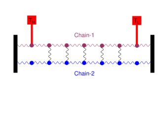
Figure 1: Schematic configuration of our approach to manipulate thermal conductivity. Chain-1 and chain-2 represent the conductive material and the substrate, respectively. The two particles on the left and right ends of chain-1 are put into contact with thermostats of temperature $T_{H}$ and $T_{L}$, respectively.

Fig. 1 shows the schematic configuration of our approach, which is illustrated by a coupled atom chain model. The upside chain (chain-1) represents the conductive material and the underside chain (chain-2) represents the substrate. The two ends of chain-1 are contacted with the thermostats with temperature $T_{H}$ and $T_{L}$, respectively, while, chain-2 is free of thermostat contact. Each node of chain-1, except for the two ends contacted with thermostat, is coupled to the corresponding underside node of chain-2. This ladder-like construction corresponds well to the real systems, where the conductive materials are always fixed on some substrates.

Two coupled FPU chains are firstly considered to represent the approach in details, with all the Hamiltonian parameters being in the reduced units.19 ; 20 In the model, the atomic mass and spring constant of chain-1 ($m_{1},k_{1}$) are fixed to be 1.0, the anharmonic coefficient of chain-1 and chain-2 ($\beta_{1}$, $\beta_{2}$) and the coupling strength $k_{c}$ are all set to be 0.5. The atomic mass and spring constant of chain-2 $(m_{2},k_{2})$ are variables to manipulate thermal conductivity of chain-1 (see Supporting Information, SI.I).

The nonequilibrium molecular dynamics (NEMD)19 ; 20 ; 22 method is used to calculate the heat flux of chain-1 and chain-2 in the coupling system. It is found that the phonon resonance between chain-1 and chain-2 plays an important role on the thermal conductivity. Here we use the resonance angle $\Psi$=$\left|\arctan(\frac{\lambda_{2}}{\lambda_{1}})\right|$ to describe the phonon resonance strength, where $\lambda_{1}$ and $\lambda_{2}$ are the phonon amplitudes of chain-1 and chain-2 after coupling (see Supporting Information, SI.II). It is obvious that the resonance strength becomes a maximum (minimum) at $\Psi$ =$\frac{\pi}{4}$($\Psi$ = $0$).

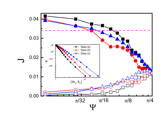
Figure 2: Heat flux of chain-1 and chain-2 with variation of resonance angle $\Psi$ in the coupling system for three cases: (a) $k_{2}$ =1, $m_{2}$ is varied; (b) $m_{2}$=1, $k_{2}$ is varied; (c) both $m_{2}$ and $k_{2}$ are varied but keeping $m_{2}$=$k_{2}$. The chain length $N$ is 50, and $T_{H}$=0.3, $T_{L}$=0.2. The solid squares, triangles, and circles represent the heat flux of chain-1 for cases (a), (b), and (c), respectively; the corresponding open ones represent heat flux of chain-2 for the three cases. The short dashed line shows the heat flux of isolated chain-1. Chain-1’s heat flux monotonously decreases with $\Psi$ increasing, which can be either larger or smaller than that of the isolated one depending on the specific $\Psi$ value. The inset shows ($m_{2}$, $k_{2}$) dependence of the resonance angle for the three cases. The resonance angle is very sensitive to the ($m_{2}$, $k_{2}$) parameters.

Fig. 2 shows heat flux $J$ of chain-1 and chain-2 with variation of the resonance angle. Since $\Psi$ is not uniquely determined by $m_{2}$ or $k_{2}$, many ($m_{2}$, $k_{2}$) sets can be corresponding to a $\Psi$ value, we mainly consider three cases: (a) $k_{2}$ =1, $m_{2}$ is varied; (b) $m_{2}$=1, $k_{2}$ is varied; (c) both $m_{2}$ and $k_{2}$ are varied but keeping $m_{2}$=$k_{2}$. For all the three cases, the heat flux of chain-1 monotonously decreases with $\Psi$ increasing, while the heat flux of chain-2 has a contrary behavior. Particularly, when the phonon resonance becomes strong enough (with $\Psi$ nearby $\frac{\pi}{4}$), heat flux of chain-1 gets much smaller than that of the isolated one ($J=0.034$), suggesting a substantial reduction of thermal conductivity23 ; when the phonon resonance becomes small enough, however, the heat flux of chain-1 gets obviously larger than that of the isolated one, showing an increment of thermal conductivity, which has not been explored so far. This interesting phenomenon shows that the thermal conductivity of conductive material can be efficiently manipulated through the substrate.

We note that the resonance angle is very sensitive to the ($m_{2}$, $k_{2}$) parameters (Inset of Fig. 2). This suggests that one can easily find a proper substrate to manipulate the thermal conductivity in the application. For example, to decrease the thermal conductivity, the substrate needs to have similar atomic mass and spring constant with the conductive material; to increase the thermal conductivity, the atomic mass and/or spring constant of substrate only needs to be several times larger than that of conductive material. Moreover, the heat-flux curves of cases (a), (b), and (c) are very close to each other, indicating that the thermal conductivity of chain-1 is insensitive to the specific type of ($m_{2}$, $k_{2}$) compositions. Thus there would be rich choices of substrate candidates for the thermal conductivity manipulation. Consequently, the present approach can be easily realized in the nanotechnologies, which provides a clear direction for designing advanced nanoelectronic and thermoelectric devices.

The reduction of thermal conductivity after coupling can be understood from the phonon-resonance effect, which induces strong phonon scattering and thus reduces the thermal conductivity.17 ; 24 ; 25 ; 26 ; 27 To understand the increment of thermal conductivity, however, we need to invoke phonon band theory. Here we consider an extreme condition, where the resonance angle is zero and the increment of thermal conductivity is maximum. From the coupling-harmonic-oscillator (CHO) model, the phonon dispersion of chain-1 in the coupling system can be written as $\omega(q)=\sqrt{\frac{k_{1}}{m_{1}}}\cdot\sqrt{4\sin^{2}(\frac{1}{2}q)+k_{c}}$. Compared with that of the isolated case $\omega(q)=2\sqrt{\frac{k_{1}}{m_{1}}}\cdot\sin(\frac{1}{2}q)$, the phonon band of chain-1 has an obvious upshift after coupling, the magnitude of which is proportional to $\sqrt{k_{c}}$ (Inset of Fig. 3).

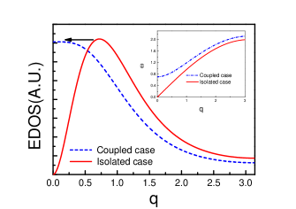
Figure 3: PED distributions with the wave vector $q$ of chain-1 in both the isolated and the coupled (with $\Psi=0$) cases at T=0.25. The PED peak has an obvious shift to the small-$q$ direction after coupling. The inset shows the corresponding phonon dispersions.

Based on the phonon dispersion, the phonon energy density (PED) distributions of chain-1 with wave vector $q$ can be further calculated (see Supporting Information, SI.III). Compared with that of isolated case, the PED peak has an obvious shift to the small-$q$ direction owning to the upshift of phonon band after coupling (Fig. 3), suggesting more energy has been carried and transported by the small-$q$ phonons. The phonons’ scattering power is proportional to the phase difference between different atoms, which is hence proportional to the $q$ value.28 More small-$q$ phonons being responsible for the heat transport corresponds to smaller scattering power, thus larger phonon mean free paths (PMFPs) in chain-1, which increases the thermal conductivity (positive effect). On the other hand, the upshift of the phonon band also results in less phonons being excited for the heat transport, which in turn reduces the thermal conductivity (negative effect). The thermal conductivity variation induced by the phonon band upshift is attributed to such two effects competing with each other (phonon-band-upshift effect).

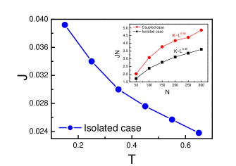
Figure 4: (a) Temperature dependence of heat flux of isolated chain-1 ($N$=50). The phonon scattering effect has become dominant at our simulation temperature (T=0.25). The inset shows chain length $N$ dependence of total heat flux $JN$ of chain-1 in both the isolated and the coupled (with $\Psi=0$) cases. The larger fitting exponent implies that the increment of thermal conductivity by the coupling gets more and more distinguished with the chain length increasing.

We have also calculated the temperature dependence of heat flux of isolated chain-1 (Fig. 4) and found the heat flux monotonically decreases with the temperature increasing from T=0.15 to 0.65. It is known that increasing temperature has two competitive effects on the thermal conductivity: (i) It excites more high-frequency phonons that enhance the thermal conductivity. (ii) It increases phonon-phonon scattering that reduces the thermal conductivity.13 ; 20 Fig. 4 shows that effect (ii) has become dominant at our simulation temperature (T=0.25), indicating that the upshift of phonon band, which has similar effect with that of decreasing temperature, has more positive effect than the negative effect on the thermal conductivity. Hence the thermal conductivity can be increased due to the phonon-band-upshift effect. Moreover, inset of Fig. 4 shows the chain length dependence of total heat flux($JN$) of chain-1 in both the coupled (with $\Psi=0$) and isolated cases. As is shown, $JN$ of the isolated chain-1 diverges as $JN\propto N^{0.4}$, consistent with the results in previous reports.19 ; 20 While, for the coupled case, $JN\propto$ $N^{0.48}$. The larger fitting exponent implies that the increment of thermal conductivity by the coupling gets more and more distinguished with the chain length increasing.

Consequently, in the coupling system, the thermal conductivity variation is owed to both the phonon-band-upshift effect and the phonon-resonance effect that compete with each other. From the results above (Fig. 2), the phonon-resonance effect can be easily manipulated by changing the atomic mass and/or spring constant of the substrate. Thus we can efficiently manipulate the thermal conductivity of conductive material through coupling it to different substrates.

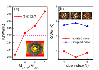
Figure 5: (a) Thermal conductivity of (7,0) CNT coupled within (14,0) CNT, with variation of (14,0) CNT’s atomic mass $M_{CNT14}$ ($M_{CNT7}$ is kept to be carbon-atom mass). The short dashed line shows the thermal conductivity value of isolated (7,0) CNT. The thermal conductivity of (7,0) CNT can be either substantially decreased or increased depending on the value of $M_{CNT14}$. The inset shows the structure of (7,0)@(14,0) DWNT. (b) Thermal conductivity of Ice-NTs. Thermal conductivity of Ice-NTs has an obvious increment after coupling. The inset shows optimized structures of ice-NTs coupled within CNTs.

As a demonstration of this approach in the real systems, we have calculated the thermal conductivity of a (7,0) carbon nanotube (CNT) coupled within (14,0) CNT as a substrate((7,0)@(14,0) DWNT, see Supporting Information, SI.IV). We set the atomic mass of (14,0) CNT ($M_{CNT14}$) as parameter to see how the thermal conductivity of (7,0) CNT changes with the resonance angle. In the coupling system, the resonance angle $\Psi$ and thus the thermal conductivity can be efficiently manipulated through changing $M_{CNT14}$. As shown in Fig. 5(a), thermal conductivity of (7,0) CNT obviously increases with $M_{CNT14}$ increasing from one to several times that of atomic mass of (7,0) CNT (carbon-atom mass, $M_{CNT7}$) owing to the reduction of phonon-resonance effect. Compared with that of the isolated case, the thermal conductivity of (7,0) CNT can be either substantially decreased or increased depending on the value of $M_{CNT14}$, consistent with the results of coupled FPU chain model, which can be well understood form the coupling mechanism discussed above. When $M_{CNT14}=M_{CNT7}$ ($\Psi\approx\frac{\pi}{4}$), the phonon-resonance effect that decreases the thermal conductivity is dominant and the thermal conductivity is decreased by coupling. With $M_{CNT14}$ increasing, the phonon-resonance effect becomes more minor. When $M_{CNT14}\geq 2M_{CNT7\text{ }}(\Psi<\frac{\pi}{32}$)29 , the phonon-band-upshift effect that increases the thermal conductivity becomes dominant, and thus the thermal conductivity is increased by coupling.

Ice-NT coupled within a CNT can be considered as another realistic illustration for our approach, where the Ice-NT and CNT correspond to the conductive material and the substrate. Since the CNTs have much larger spring constant than the Ice-NTs (from Supporting Information,$\Psi\sim 0$), an increment of thermal conductivity of Ice-NTs is expected after coupling with CNTs. Fig. 5(b) shows the calculated thermal conductivity of various Ice-NTs both with and without CNT coupling (see Supporting Information, SI.V). As one can see, the thermal conductivity of Ice-NTs has an obvious increment after coupling, which is independent on the specific tube types. These realistic illustrations further confirm the feasibility of our approach for applications.

In summary, we have proposed a new approach to manipulate the thermal conductivity. By coupling with different substrates, thermal conductivity of the conductive nanomaterial can be either remarkably decreased or increased, which can be realized in the device applications. To decrease the thermal conductivity, the substrate needs to have similar atomic mass and spring constant with the conductive material; to increase the thermal conductivity, the atomic mass and/or spring constant of the substrate needs to be several times larger than that of the conductive material. Through the illustrations of double-walled carbon nanotubes and coupled ice nanotubes, we have further shown that this approach is applicable in the real systems. Compared with the conventional treatments which only reduce the thermal conductivity, our approach can truly realize the thermal conductivity manipulation in solid nanomaterials without destroying their structures.

Acknowledgments:

We gratefully thank Z. Y. Zhang and S. H. Wei for fruitful discussions. This work was partially supported by the Special Funds for Major State Basic Research, National Science Foundation of China, Ministry of education and Shanghai municipality. The computation was performed in the Supercomputer Center of Shanghai, the Supercomputer Center of Fudan University.

I Supporting Information

”Manipulating thermal conductivity through substrate coupling”, Zhixin Guo, Dier Zhang, and Xin-Gao Gong

SI.I Hamiltonian of the coupled FPU chains

The Hamiltonian of the coupled FPU chain model can be written as:

$$H=H_{1}+H_{2}+H_{c},$$ (1)

$$H_{n}=\underset{i}{\sum}\left[\frac{(p_{n}^{i})^{2}}{m_{n}}+\frac{1}{2}k_{n}(x_{n}^{i}-x_{n}^{i-1})^{2}+\frac{1}{4}\beta_{n}(x_{n}^{i}-x_{n}^{i-1})^{4}\right],(n=1,2),$$ (2)

$$H_{c}=\underset{i}{\sum}\left[\frac{1}{2}k_{c}(x_{2}^{i}-x_{1}^{i})^{2}\right],$$ (3)

where $H_{1},H_{2},$ and $H_{c}$ are the Hamiltonian of chain-1, chain-2, and the coupling term, respectively. $x_{n}^{i}$ , $p_{n}^{i}$ represent the displacement from the equilibrium position, the momentum of the $ith$ particle; and $m_{n}$, $k_{n}$, $\beta_{n}$ are the mass, spring constant and the anharmonic coefficient of chain-$n$ $(n=1,2)$.

SI.II Definition of resonance angle $\Psi$

Using the coupling-harmonic-oscillator (CHO) model, we can calculate the phonon resonance strength. The amplitude ratio of chain-2 and chain-1 after coupling can be expressed as:

$$\frac{\lambda_{2}}{\lambda_{1}}=\sqrt{\frac{m_{1}}{m_{2}}}\tan(\alpha)\ (m_{2}\geq m_{1}),$$ (4)

where $\lambda_{1}$ and $\lambda_{2}$ are the amplitudes of chain-1 and chain-2, respectively. Here $\tan(\alpha)=\frac{(\omega_{1}-\omega_{2})\pm\sqrt{(\omega_{1}-\omega_{2})^{2}+4\omega_{c}^{2}}}{2\omega_{c}}\in[-1,1]$, and $\omega_{c}=$ $\frac{k_{c}}{\sqrt{m_{1}m_{2}}},$ $\omega_{1}=$ $\frac{k_{1}+k_{c}}{m_{1}},\omega_{2}=$ $\frac{k_{2}+k_{c}}{m_{2}}$, respectively. Then the resonance angle is defined as $\Psi=\left|\arctan(\frac{\lambda_{2}}{\lambda_{1}})\right|$. When $\Psi=0,$ the phonon dispersion of chain-1 in the coupling system can be written as:

$$\omega(q)=\sqrt{\frac{k_{1}}{m_{1}}}\cdot\sqrt{4\sin^{2}(\frac{1}{2}q)+k_{c}},$$ (5)

Thus the phonon band of chain-1 has an obvious upshift after coupling, the magnitude of which is proportional to $\sqrt{k_{c}}$.

SI.III Calculation of PED distribution with wave vector

Figure 6: PED distributions with phonon frequency $\omega$ of isolated chain-1 at T=0.25.

The $q$ dependence of PED has an expression of $u(q)=\hbar\omega(q)\times\eta[\omega(q),T],$with $\eta[\omega(q),T]$ representing the phonon distribution function at temperature $T$ for a certain frequency $\omega$. Since the phonon distribution in a heat-transport system is mainly determined by the heat source that supplies phonons. We suppose the conductive chain is coupled to an ideal heat source that supplies phonons like the black-body, which can be represented by the Nosé-Hoover thermostat1 ; 2 . Then $\eta(\omega,T)$ can be written as:

$$\eta(\omega,T)=\frac{8\pi\omega^{2}}{c^{3}}\frac{1}{e^{\hbar\omega/k_{b}T}-1},$$ (6)

Using equation (6), we also calculated the PED distributions with phonon frequency $\omega$ of the isolated chain-1. As is shown in Fig. 1, the result is consistent with that calculated by Li et al. using the numerical method, which confirms the reliability of our consideration.3

SI.IV NEMD simulation for the double-walled carbon nanotube

In the simulation, the Tersoff potential was used to the describe the carbon-carbon interaction4 , and the coupling interaction between two CNTs was described by the LJ potential,5 which was truncated at 10 Å by a switching function. The simulated (7,0)@(14,0) DWNT has a length of 121 Å, containing 2352 atoms. The wall-thickness of CNT was chosen to be 1.44 Å for the calculation of cross-section area.6 ; 7 Fixed boundary condition was applied along the axial direction of CNTs, where the outmost two layers of each head were fixed.7 ; 8 Then two layers of each end of (7,0) CNT were put into contact with the Nosé-Hoover thermostat with temperatures 310 and 290 K, respectively, while the (14,0) CNT was free of thermostat contact. To integrate equations of motion, the velocity Verlet method was employed with a fixed time step of 1 $fs$. All results were obtained by averaging about $10\ ns$ after a sufficient long transient time ($10\ ns$) to set up a nonequilibrium stationary state.

SI.V NEMD simulation for the Ice-NTs

Water-water intermolecular interaction was described by the TIP4P9 potential and carbon-carbon interaction was described by the Tersoff4 potential. As for the coupling term, the CNT-water interaction was described by a carbon-oxygen LJ potential.10 All the pair interactions were truncated at 10 Å by a switching function. The simulation box has a length of 121 Å and the total number of water molecules inside is 44$\times$n for the (n,0) Ice-NT, where n = 4, 5, and 6. The Ice-NTs’ wall-thickness was chosen to be 2.75 Å for the calculation of cross-section area11 . Fixed boundary condition was applied along the axial direction of Ice-NT/CNT, where the outmost two layers of each head were fixed.7 ; 8 Then two layers of each end of Ice-NT were put into contact with the Nosé-Hoover thermostat with temperatures 110 and 90 K, respectively, while the CNT was free of thermostat contact. To integrate equations of motion, the velocity Verlet method was employed with a fixed time step of 1 $fs$. All results were obtained by averaging about $5\ ns$ after a sufficient long transient time ($5\ ns$) to set up a nonequilibrium stationary state.

References

- (1) Collins, P. G.; Zettl, A.; Bando, H.; Thess, A.; Smalley, R. E. Science 1997, 278, 100-103.
- (2) Huang, X. M. H.; Zorman, C. A.; Mehregany, M.; Roukes, M. L. Nature 2003, 421, 496-496.
- (3) Huang, Y.; Duan, X.; Cui, Y.; Lauhon, L. J.; Kim, K. H.; Lieber, C. M. Science 2001, 294, 1313-1317.
- (4) Li, M.; Pernice, W. H. P.; Tang, H. X. Nature Nanotech. 2009, 4, 377-382.
- (5) Chen, G.; Dresselhaus, M. S.; Dresselhaus, G.; Fleurial, J. P.; Caillat, T. Int. Mater. Rev. 2003, 48, 45-66.
- (6) Dresselhaus, M. S.; Chen, G.; Ren, Z. F.; Dresselhaus, G.; Henry, A.; Fleurial, J. P. JOM 2009, 61, 86-90.
- (7) Dresselhaus, M. S.; Chen, G.; Tang, M. Y.; Yang, R.; Lee, H.; Wang, D.; Ren, Z.; Fleurial, J. P.; Gogna, P. Adv. Mater. 2007, 19, 1043-1053 .
- (8) Cahill, D. G.; Ford, W. K.; Goodson, K. E.; Mahan, G. D.; Majumdar, A.; Maris, H. J.; Merlin, R. ; Phillpot, S. R. J. Appl. Phys. 2003, 93, 793-818.
- (9) Ghosh, S.; Calizo, I.; Teweldebrhan, D.; Pokatilov, E. P.; Nika, D. L.; Balandin, A. A.; Bao, W.; Miao, F.; Lau, C. N. Appl. Phys. Lett. 2008, 92, 151911.
- (10) Biercuk, M. J.; Llaguno, M. C.; Radosavljevic, M.; Hyun, J. K.; Johnson, A. T. Appl. Phys. Lett. 2002, 80, 2767-2769.
- (11) Yang, N.; Zhang, G.; Li, B. Nano Lett. 2008, 8, 276-280.
- (12) Samvedi, V.; Tomara, V. J. Appl. Phys. 2009, 105, 013541.
- (13) Zhang, G.; Li, B. J. Chem. Phys. 2005, 123, 114714.
- (14) Padgett, C. W.; Brenner, D. W. Nano Lett. 2004, 4, 1051-1053.
- (15) Donadio, D.; Galli, G. Phys. Rev. Lett. 2007, 99, 255502.
- (16) Seol, J. H.; Jo, I.; Moore, A. L.; Lindsay, L.; Aitken, Z. H.; Pettes, M. T.; Li, X.; Yao, Z.; Huang, R.; Broido, D.; Mingo, N.; Ruoff, R. S.; Shi, L. Science 2010, 328, 213-216.
- (17) Ghosh, S.; Bao, W.; Nika, D. L.; Subrina, S.; Pokatilov, E. P.; Lau, C. N.; Balandin,A. A. Nature Mater. 2010, 9, 555-558.
- (18) Savin, A. V.; Kivshar, Y. S.; Hu, B. Europhys. Lett. 2009, 88, 26004.
- (19) Lepri, S.; Livi, R.; Politi, A. Phys. Rep. 2003, 377, 1-80.
- (20) Hu, B.; Li, B.; Zhao, H. Phys. Rev. E 1998, 57, 2992-2995.
- (21) Koga, K.; Gao, G. T.; Tanaka, H.; Zeng, X. C. Nature 2001, 412, 802-805.
- (22) Mai, T.; Dhar, A.; Narayan, O. Phys. Rev. Lett. 2007, 98, 184301.
- (23) Since the temperature difference is fixed to be 0.1, from the Fourier law, the thermal conductivity is proportional to the heat flux value.
- (24) Yan, X. H.; Xiao, Y.; Li, Z. M. J. Appl. Phys. 2006, 99, 124305.
- (25) Pohl, R. O. Phys. Rev. Lett. 1962, 8, 481-483.
- (26) Tse, J. S.; Shpakov, V. P.; Belosludov, V. R.; Trouw, F.; Handa Y. P.; Press, W. Europhys. Lett. 2001, 54, 354-360.
- (27) Krivchikov, A. I.; Yushchenko, A. N.; Korolyuk, O. A.; Bermejo, F. J.; Fernandez-Perea, R.; Bustinduy, I.; González, M. A. Phys. Rev. B 2008, 77, 024202.
- (28) Prasher, R. J. Heat Transfer 2006, 128, 627-637.
- (29) From the Tersoff potential, we evaluated the spring constant of C-C bond of CNTs (corresponding to and of the coupled FPU chain model) to be about 1250 N/m. From LJ potential, the CNT-CNT intertube coupling spring constant (corresponding to of the coupled FPU chain model) was evaluated to be about 33 N/m. Then from the Supporting Information, SI.II, we get .

References

- (1) Nosé, S. J. Chem. Phys. 1984, 81, 511-519.
- (2) Hoover, W. G. Phys. Rev. A 1985, 31, 1695-1697.
- (3) Li, B., Lan, J.; Wang, L. Phys. Rev. Lett. 2005, 95, 104302.
- (4) Tersoff, J. Phys. Rev. B 1989, 39, 5566-5568.
- (5) Girifalco, L. A.; Hodak, M.; Lee, R. S. Phys. Rev. B 2000, 62, 13104-13110.
- (6) Zhang, G.; Li, B. J. Chem. Phys. 2005, 123, 114714.
- (7) Guo, Z.; Zhang, D.; Gong, X. G. Appl. Phys. Lett. 2009, 95, 163103.
- (8) Wu, G.; Li, B. Phys. Rev. B 2007, 76, 085424.
- (9) Jorgensen, W. L.; Chandrasekhar, J.; Madura, J. D.; Impey, R. W.; Klein, M. L. J. Chem. Phys. 1983, 79, 926-935.
- (10) Meng, L.; Li, Q.; Shuai, Z. J. Chem. Phys. 2008, 128, 134703.
- (11) Guo, Z.; Zhang, D.; Zhai, Y.; Gong, X. G. Nanotechnology 2010, 21, 285706.