New method for the quantum ground states in one dimension

Abstract

A simple, general and practically exact method is developed to calculate the ground states of 1D macroscopic quantum systems with translational symmetry. Applied to the Hubbard model, a modest calculation reproduces the Bethe Ansatz results.

Since the very beginning of the quantum theory, to solve the Schrödinger equation for macroscopic quantum systems has been one of the main tasks of theoretical physics. It would not be an exaggeration to say that, due to lack of such methods, a considerable effort of theoretical physicists has been devoted to the development of a variety of perturbative and approximate methods and numerical simulations. But a desire for powerful non-perturbative methods has grown stronger over the last couple of decades with the list of phenomena played by strongly correlated electrons getting longer, particularly since the discovery of high temperature superconductivity in copper oxides J.G.Bednorz and K.A.Müller (1986). While we have seen a considerable progress in rigorous treatment of quantum 1D and classical 2D systems over the last several decades L.Onsager (1944); C.N.Yang (1952); B.M.McCoy and T.T.Wu (1973); R.J.Baxter (1989); N.Andrei et al. (1983); S.G.Chung et al. (1983); E.H.Lieb and F.Y.Wu (1968); Sutherland (2004), these rigorous methods are not flexible enough to solve non-integrable models in one dimension, nor, most probably, generalizable to higher dimensions. On the other hand, the method of NRG (numerical renormalization group), particularly DMRG (density matrix RG) has seen a remarkable success first in quantum 1D systems S.R.White (1993) and then in finite Fermi systems, competing well with the conventional quantum chemistry calculations Dukellsky and Pittel (2004). More recently, the notion of entanglement from quantum information theory M.A.Nielsen and I.L.Chuang (2000) helped a further progress in NRG towards the finite temperature as well as dynamical quantities M.Zwolak and G.Vidal (2004); V.Murg et al. (2005); S.R.White and A.E.Feiguin (2004).

In a recent article, we have developed a simple, general and practically exact method to calculate statistical mechanical properties of macroscopic classical systems with translational symmetry up to three dimensions S.G.Chung (in press, available online). We here extend this method to solve the Schrödinger equation for 1D quantum ground states with translational symmetry. As a benchmark model for this development, we consider the Hubbard model. Just like our recent work on the 3D Ising model, our method is purely algebraic and other than seeking a convergence in entanglement space, it does not employ any other notions such as NRG, nor make any approximations. Our results for the ground state energy and the local magnetic moment in the 1D Hubbard model agree with the known exact results by Bethe Ansatz H.Shiba (1972); E.H.Lieb and F.Y.Wu (1968). An important difference of the present method from the Bethe Ansatz, however, should be emphasized: the new method is not rigorous but mathematically much simpler, general and therefore readily applicable to any quantum spins, fermions and bosons. This is a reflection of the fact that our recent method for the Ising model is applicable to any classical statistical systems with translational symmetry. Yet another but probably the most significant remark here is that the success in 1D Hubbard model should constitute an essential ingredient in the analysis of the 2D Hubbard model by the present method. Again, this is a reflection of the fact that our recent method for the 3D Ising model crucially relies on the successful analysis of the 2D Ising model, we called it the ”Russian doll” structure, and the mathematical structure involving the D=2,3 Ising models and that for the D=1,2 Hubbard models are essentially identical.

The Hubbard model is defined by the Hamiltonian,

$$H=-t\sum_{\sigma,<ij>}(c_{i\sigma}^{\dagger}c_{j\sigma}+h.c.)+U\sum_{i}n_{i\uparrow}n_{i\downarrow}$$ (1)

where $t$ is the tranfer integral, a measure of kinetic energy, $U$ is the onsite Coulomb potential and $c_{i\sigma}$, $c_{i\sigma}^{\dagger}$ are the annihiration and creation operators for electrons at site $i$ and spin $\sigma$. We take $t$ as the energy unit. To calculate the ground state of the Schrödinger equation

$$H\Psi=E\Psi$$ (2)

we follow the following steps.

First, instead of (2), consider the eigenvalue problem for the density matrix

$$e^{-\beta H}\Psi=e^{-\beta E}\Psi$$ (3)

A well-known observation about (3) is that, starting with a trial wavefunction $\Psi$ which has non-zero overlap with the ground state, only the ground state survives in the limit $\beta\rightarrow\infty$. Monte Carlo and NRG simulations are based on this observation M.Suzuki (1993); S.R.White (1993). Here our idea goes opposite, $\beta\rightarrow 0$, and calculate the largest eigenvalue of the operator $1-\beta H$ and corresponding eigenstate.

Second, we rewrite the Hamiltonian (1) as a sum of a local bond Hamiltonian,

$$H=\sum_{bond}(H_{ij}+H_{i}+H_{j})\equiv\sum_{bond}H_{bond}$$ (4)

with

$$H_{ij}=-t\sum_{\sigma,<ij>}(c_{i\sigma}^{\dagger}c_{j\sigma}+h.c.)$$ (5)

$$H_{i}=\frac{U}{2}n_{i\uparrow}n_{i\downarrow}-\frac{\mu}{2}(n_{i\uparrow}+n_{i\downarrow})$$ (6)

where the onsite Coulomb term is split into two sites $i$ and $j$, and the chemical potential $\mu$ is introduced to control the electron number per site.

Third, we note a decomposition of the density matrix,

$$e^{-\beta H} = \Pi_{bond}e^{-\beta H_{bond}}+\mathcal{O}(\beta^{2})$$ (7)

$$\approx e^{-\beta\sum_{even}{H_{bond}}}e^{-\beta\sum_{odd}{H_{bond}}}$$

This is the simplest Suzuki-Trotter decomposition M.Suzuki (1976), but it is good enough for $\beta\rightarrow 0$. In (7), following the procedure familiar in quantum Monte Carlo, we have split the entire bonds into two groups: one connecting the sites $(2i,2i+1)$, the even group, and the other $(2i+1,2i+2)$, the odd group. Now the local bond density matrix should be further decomposed as,

$$e^{-\beta H_{bond}} \approx e^{-\beta H_{i}}e^{-\beta H_{j}}e^{-\beta H_{ij}}$$ (8)

$$\approx [1-\frac{\beta U}{2}n_{i\uparrow}n_{i\downarrow}+\frac{\beta\mu}{2}(n_{i\uparrow}+n_{i\downarrow})]\cdot[i\rightarrow j]$$

$$+\beta t\sum_{\sigma}(c_{i\sigma}^{\dagger}c_{j\sigma}+h.c.)$$

$$\equiv \Omega_{\alpha}\otimes\Theta_{\alpha}$$

where and below the repeated indices imply a summation, and $\Omega_{\alpha}$ takes five operators, $1-\frac{\beta U}{2}n_{i\uparrow}n_{i\downarrow}+\frac{\beta\mu}{2}(n_{i\uparrow}+n_{i\downarrow})$, $c_{i\uparrow}^{\dagger}$, $c_{i\uparrow}$, $c_{i\downarrow}^{\dagger}$, and $c_{i\downarrow}$ and $\Theta_{\alpha}$ likewise operators at site $j$. Since the local pair density matrix (8) contains even number of creation and annihiration operators, the matrix representation of the density matrix (7) can be written as a operator product of local matrices,

$$\langle lk|e^{-\beta H_{bond}}|ij\rangle\approx f_{\alpha,ik}\otimes g_{\alpha,jl}$$ (9)

where

$$f_{1}=g_{1}=\left(\begin{array}[]{clcr}1&0&0&0\\ 0&\beta\mu/2&0&0\\ 0&0&\beta\mu/2&0\\ 0&0&0&-\beta U/2+\beta\mu\end{array}\right)$$

$$f_{2}=\sqrt{\beta t}\left(\begin{array}[]{clcr}0&0&0&0\\ 1&0&0&0\\ 0&0&0&0\\ 0&0&-1&0\end{array}\right)$$

$$g_{2}=\sqrt{\beta t}\left(\begin{array}[]{clcr}0&1&0&0\\ 0&0&0&0\\ 0&0&0&1\\ 0&0&0&0\end{array}\right)$$

etc., where four basis states at each site are ordered as $|0\rangle$, $|\uparrow\rangle$, $|\downarrow\rangle$ and $|\uparrow\downarrow\rangle$. Note that the $-1$ in the $f_{2}$ matrix is due to the fermion anticommutation algebra. Thus the matrix product representation of the even group bonds in the density matrix is,

$$\cdots f_{\alpha}\otimes g_{\alpha}\otimes f_{\beta}\otimes g_{\beta}\otimes f_{\gamma}\otimes g_{\gamma}\cdots$$ (10)

and the same expression for the odd group bonds with one lattice shifted from the even group case. Putting together, we have the matrix representation of the density matrix (7) as,

$$K \equiv \cdots\otimes g_{\alpha}\cdot f_{\beta}\otimes f_{\gamma}\cdot g_{\beta}\otimes g_{\gamma}\cdot f_{\delta}\otimes$$ (11)

$$~{}~{}~{}~{}~{}~{}~{}~{}~{}~{}f_{\varepsilon}\cdot g_{\delta}\otimes g_{\varepsilon}\cdot f_{\nu}\otimes\cdots$$

$$\equiv \cdots\Gamma_{\alpha\beta}^{1}\otimes\Gamma_{\beta\gamma}^{2}\otimes\Gamma_{\gamma\delta}^{1}\otimes\Gamma_{\delta\varepsilon}^{2}\cdots$$

where for notational simplicity, we have raised the indices $1,2$ for the two $\Gamma s$ to their shoulders. Note also that $\Gamma_{\alpha\beta}^{1,2}$ are $4{\rm x}4$ matrices for each pair of interaction indices $(\alpha,\beta)$. Thus, $\Gamma^{1,2}$ are a set of $5^{2}{\rm x}4^{2}$ numbers which will be denoted below like $\Gamma_{abcd}^{1,2}$, where $(a,b)$ indicates (up,down) interaction channels, whereas $(c,d)$ indicates (left,right) basis states.

Figure 1: Schematic figure of the transfer matrix eigenvalue equation, Eq(3).

Fourth, we write the ground state wavefunction as,

$$\Psi=\cdots\zeta_{\alpha\beta a_{1}}^{1}\otimes\zeta_{\beta\gamma a_{2}}^{2}\otimes\zeta_{\gamma\delta a_{3}}^{1}\otimes\zeta_{\delta\varepsilon a_{4}}^{2}\cdots$$ (12)

on the basis $\cdots|a_{1}\rangle\otimes|a_{2}\rangle\otimes|a_{3}\rangle\otimes|a_{4}\rangle\otimes\cdots$ where $a_{1}$ etc takes 4 states $|0\rangle$, $|\uparrow\rangle$, $|\downarrow\rangle$ and $|\uparrow\downarrow\rangle$. One can derive the form (12) by a successive use of matrix algebra S.G.Chung (in press, available online). Consider, for example, a wave function $\Psi(a_{1}a_{2}a_{3}a_{4})$. Regarding this as a matrix of the left index $a_{1}$ and the right index $\{a_{2}a_{3}a_{4}\}$, SVD (singular value decomposition) gives $\Psi(a_{1}a_{2}a_{3}a_{4})=\sum_{\alpha}{A_{a_{1}\alpha}\rho_{\alpha}B_{\{a_{2}a_{3}a_{4}\}\alpha}}$. The quantity $B$ can in turn be regarded as a matrix of the left index $\{a_{2}\alpha\}$ and the right index $\{a_{3}a_{4}\}$, thus SVD gives $B_{\{a_{2}a_{3}a_{4}\}\alpha}=\sum_{\beta}{C_{\{a_{2}\alpha\}\beta}\lambda_{\beta}D_{\{a_{3}a_{4}\}\beta}}$. Likewise, $D_{\{a_{3}a_{4}\}\beta}=\sum_{\gamma}{E_{\{a_{3}\beta\}\gamma}\Delta_{\gamma}F_{a_{4}\gamma}}$. Putting together, rewriting $A_{a_{1}\alpha}$ as $A_{\alpha}(a_{1})$, $C_{\{a_{2}\alpha\}\beta}$ as $C_{\alpha\beta}(a_{2})$, $E_{\{a_{3}\beta\}\gamma}$ as $E_{\beta\gamma}(a_{3})$ and $F_{a_{4}\gamma}$ as $F_{\gamma}(a_{4})$, and appropriately absorbing $\rho_{\alpha}$, $\lambda_{\beta}$ and $\Delta_{\gamma}$ into the matrices $A$, $C$, $E$ and $F$, one gets $\Psi(a_{1}a_{2}a_{3}a_{4})=A_{\alpha}(a_{1})C_{\alpha\beta}(a_{2})E_{\beta\gamma}(a_{3})F_{\gamma}(a_{4})$. For our density matrix with a bipartite structure with translational symmetry, (11), one arrives at the claimed form. Again for notational simplicity, we have raised the indices $1,2$ for the two $\zeta s$ to their right shoulders. In quantum information theory, these indices $\alpha$, $\beta$ and $\gamma$ are known as entanglement M.A.Nielsen and I.L.Chuang (2000). Considering only 1 for these indices is a simple mean-field-like approximation for $\Psi$. Allowing larger values, one takes into account the effect of correlation with increasing precision. An important note here is that (12) is not peculiar to the Hubbard model, but rather a general statement for macroscopic quantum ground states with translational symmetry. Putting the above arguments together, the eigenvalue problem (3) for $\beta\rightarrow 0$ is then written schematically as in Fig. 1. The horizontal lines indicate 4 local basis states, whereas the vertical lines indicate 5 interaction channels connecting nearest neighbor sites for $\Gamma^{1,2}$ and entanglements for $\zeta^{1,2}$. To emphasize the close similarity to our recent analysis of the Ising model, let us call all 4 lines associated with $\Gamma^{1,2}$ as bonds. Note that Fig. 1 is a slight generalization of Fig. 1 in the 2D Ising model S.G.Chung (in press, available online).

Fifth, we follow the procedure in our method for the Ising model, namely we handle the eigenvalue problem (3) as a variational problem. We thus maximize the quantity $\mu_{0}=\Psi K\Psi/\Psi\Psi$ by iteration starting with an input state for $\Psi$. First consider the numerator. A local ingredient of this quantity is, $A_{ll^{\prime}e,mm^{\prime}f}\equiv\zeta_{ln\alpha}^{1}\Gamma_{eg\alpha\alpha^{\prime}}^{1}\zeta_{l^{\prime}n^{\prime}\alpha^{\prime}}^{1}\zeta_{nm\beta}^{2}\Gamma_{gf\beta\beta^{\prime}}^{2}\zeta_{n^{\prime}m^{\prime}\beta^{\prime}}^{2}$. The real nonsymmetric matrix $A$ can be written as $A=R\nu L^{tr}$ where the matrices $L$, $R$, and $\nu$ are made up of left eigenvectors, right eigenvectors and eigenvalues of $A$ and $tr$ means the transpose. The eigenvectors are normalized as $L^{tr}\cdot R=1$, and due to this property, the summation over the combined entanglement-bond indices $ll^{\prime}e$ in the numerator can be done $N-1$ times, $N\rightarrow\infty$ in the end, and thus we only keep the largest eigenvalue $\nu_{0}$ and eigenvectors ${\bf L_{0}}$ and ${\bf R_{0}}$. We have $\Psi K\Psi=\nu_{0}^{N-1}{\bf L_{0}}^{tr}A{\bf R_{0}}$. The denominator is handled likewise. Let us denote the corresponding largest eigenvalue and eigenvector as $\rho_{0}$, ${\bf\tilde{L}_{0}}$ and ${\bf\tilde{R}_{0}}$. Note that $\mu_{0}$ now contains $\zeta^{1,2}$ in a quadratic form. Maximizing this quantity with respect to $\zeta^{1}$ and $\zeta^{2}$ then leads to generalized eigenvalue problems:

$$\mathcal{S}\{{\bf L_{0}}(mm^{\prime}f){\bf R_{0}}(ll^{\prime}e)\Gamma_{fg\alpha\alpha^{\prime}}^{1}\Gamma_{ge\beta\beta^{\prime}}^{2}\zeta_{nl\beta}^{2}\zeta_{n^{\prime}l^{\prime}\beta^{\prime}}^{2}\}\zeta_{mn\alpha}^{1}$$ (13)

$$= \tilde{\mu}_{0}\mathcal{S}\{{\bf\tilde{L}_{0}}(mm^{\prime}){\bf\tilde{R}_{0}}(ll^{\prime})\delta_{\alpha\alpha^{\prime}}\delta_{\beta\beta^{\prime}}\zeta_{nl\beta}^{2}\zeta_{n^{\prime}l^{\prime}\beta^{\prime}}^{2}\}\zeta_{mn\alpha}^{1}$$

$$\mathcal{S}\{{\bf L_{0}}(mm^{\prime}f){\bf R_{0}}(ll^{\prime}e)\Gamma_{fg\alpha\alpha^{\prime}}^{1}\Gamma_{ge\beta\beta^{\prime}}^{2}\zeta_{mn\alpha}^{1}\zeta_{m^{\prime}n^{\prime}\alpha^{\prime}}^{1}\}\zeta_{nl\beta}^{2}$$ (14)

$$= \tilde{\mu}_{0}\mathcal{S}\{{\bf\tilde{L}_{0}}(mm^{\prime}){\bf\tilde{R}_{0}}(ll^{\prime})\delta_{\alpha\alpha^{\prime}}\delta_{\beta\beta^{\prime}}\zeta_{mn\alpha}^{1}\zeta_{m^{\prime}n^{\prime}\alpha^{\prime}}^{1}\}\zeta_{nl\beta}^{2}$$

where the symbol $\mathcal{S}$ means a matrix symmetrization and $\mu_{0}=\tilde{\mu}_{0}\nu_{0}^{N-1}/\rho_{0}^{N-1}$. We solve (13) and (14) for the next $\zeta^{1,2}$ and continue until convergence.

Finally after the convergence, we can calculate various ground state properties. In the present case, quantities of interest are, the average number of up spins $\langle n_{\uparrow}\rangle$, that of down spins $\langle n_{\downarrow}\rangle$, the double occupancy $\langle n_{\uparrow}n_{\downarrow}\rangle$, the kinetic energy per site $-t\sum_{\sigma}\langle c_{i\sigma}^{\dagger}c_{j\sigma}+h.c.\rangle$, and the local magnetic moment $\langle(\frac{1}{2}\vec{\sigma})^{2}\rangle$, where $\vec{\sigma}$ is the Pauli spin matrix. In general, the expectation value for the two operators $\hat{A}$ and $\hat{B}$ sitting on the adjacent sites is calculated as,

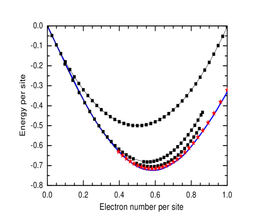
Figure 2: The ground state energy per site at $U=8$ vs. the electron number per site, $n=1$ corresponding to half-filling. From the top, the entanglement $n$=1,4,6 (rectangles) and 8 (star, red online). The thick solid line (blue online) is the Bethe Ansatz result H.Shiba (1972).

$$\langle\hat{A}\hat{B}\rangle = \Psi\hat{A}\hat{B}\Psi/\Psi\Psi$$ (15)

$$= \langle a_{2}a_{1}|\hat{A}\hat{B}|a_{1}^{\prime}a_{2}^{\prime}\rangle\zeta_{\alpha\beta a_{1}}^{1}\zeta_{\alpha^{\prime}\beta^{\prime}a_{1}^{\prime}}^{1}\zeta_{\beta\gamma a_{2}}^{2}\zeta_{\beta^{\prime}\gamma^{\prime}a_{2}^{\prime}}^{2}$$

$$B_{\gamma\gamma^{\prime},\delta\delta^{\prime}}B_{\delta\delta^{\prime},\varepsilon\varepsilon^{\prime}}\cdots B_{\varepsilon\varepsilon^{\prime},\alpha\alpha^{\prime}}/\Psi\Psi$$

where

$$B_{\gamma\gamma^{\prime},\delta\delta^{\prime}}\equiv\zeta_{\gamma\eta a_{3}}^{1}\zeta_{\gamma^{\prime}\eta^{\prime}a_{3}}^{1}\zeta_{\eta\delta a_{4}}^{2}\zeta_{\eta^{\prime}\delta^{\prime}a_{4}}^{2}$$ (16)

In fact, the matrix $B$ is nothing but the ingredient of the denominator for $\mu_{0}$, $\Psi\Psi$, and the right and left eigenvector matrices are introduced above as $\tilde{R}$ and $\tilde{L}$ and the eigenvalue matrix as $\rho$. We can write as $B=\tilde{R}\rho\tilde{L}^{tr}$, and again using the property $\tilde{L}^{tr}\cdot\tilde{R}=1$, we have, in the limit $N\rightarrow\infty$, $B^{N-1}={\bf\tilde{R}_{0}}\rho_{0}^{N-1}{\bf\tilde{L}_{0}}^{tr}$. We finally have,

$$\langle\hat{A}\hat{B}\rangle = \langle a_{2}a_{1}|\hat{A}\hat{B}|a_{1}^{\prime}a_{2}^{\prime}\rangle{\bf\tilde{R}_{0}}(\gamma\gamma^{\prime}){\bf\tilde{L}_{0}}(\alpha\alpha^{\prime})/\rho_{0}$$ (17)

$$\zeta_{\alpha\beta a_{1}}^{1}\zeta_{\alpha^{\prime}\beta^{\prime}a_{1}^{\prime}}^{1}\zeta_{\beta\gamma a_{2}}^{2}\zeta_{\beta^{\prime}\gamma^{\prime}a_{2}^{\prime}}^{2}$$

The numerical parameter used is, $\beta=10^{-6}$. The case $\beta=10^{-7}$ gives negligible corrections to the entanglement $n=3$ results below. The convergence criterion is $\|\zeta_{old}^{i}-\zeta_{new}^{i}\|/\|\zeta_{old}^{i}\|\leq 5\cdot 10^{-5}$. When this condition is met, the relative change in the largest eigenvalue $\mu_{0}$ often hits $10^{-15}$, the machine precision.

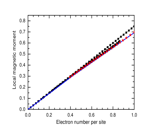
Figure 3: The same as Fig.2 for the local magnetic moment. The thick solid line (blue online) is the Bethe Ansatz result H.Shiba (1972).

Fig. 2 shows the ground state energy at $U=8$ as a function of the electron concentration, $n=1$ corresponding to half-filling. With the increase of the entanglement $n=1,4,6$ and $8$, our result converges to the Bethe Ansatz result H.Shiba (1972). Fig. 3 shows the local magnetic moment at $U=8$ as a function of the electron concentration. Again, our calculation converges to the Bethe Ansatz result H.Shiba (1972). Fig. 4 shows the ground state energy at half-filling as a function of $U$. The results are from the top, $n=1,2,3,5$ and $7$. There is a couple of % discrepancy at $U\leq 1$ from the Bethe Ansatz result E.H.Lieb and F.Y.Wu (1968). We have carried out the calculation for $n=9$ and $10$ for $U=0.01$ (took about 10 hours using a single PC of about 1 GHz processing speed) to get the ground state energy per site -1.25 and -1.255 to be compared with the exact one -1.2717. A rather slow convergence at $U\leq 1$ is a little surprise at first, but is understandable if we remember that the kinetic energy term promotes electron itinerancy, whereas the onsite Coulomb repulsion promotes electron localization. When purely itinerant, $U=0$, the ground state is constructed by filling all the momentum states up to the Fermi level, giving the ground state energy $-4/\pi$ at half-filling. If the free electron ground state is put in our form (12), we would need a large entanglement number. On the other hand, when $U\rightarrow\infty$, it is known from Bethe Ansatz that the ground state energy is $0$ at half-filling H.Shiba (1972), which is just our result with entanglement $1$. In other word, the electron is fully localized and the mean-field treatment is good enough except its wrong, but not remotely wrong, prediction of antiferromagnetic long-range order, namely the Néel state. This is a delicate issue. In fact, in the limit $U\rightarrow\infty$, the 1D Hubbard model can be mapped onto the spin one-half antiferromagnetic Heisenberg chain which does not have long-range order. But the system is critical or quasi-long-range ordered in that its correlation functions fall off as a power of the distance E.Fradkin (1991). In real materials, no truly 1D quantum or 2D classical systems exist. There always exist 3D characters such as weak inter-chain or inter-layer couplings. Although weak compared to intra-chain or intra-layer interactions, these interactions are decisive for stabilizing the long-range order.

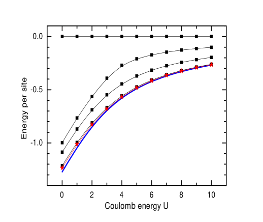
Figure 4: The ground state energy per site at half-filling as a function of the Coulomb energy $U$. From the top, the entanglement $n$=1,2,3,5 (rectangles) and 7 (star, red online). The thick solid line (blue online) is the Bethe Ansatz result E.H.Lieb and F.Y.Wu (1968).

In conclusion, the essence of the new method shall be summarized and possible future directions be discussed. First, the method is simple, general, not relying on existing methods such as the cluster mean field theories and NRG. It only uses matrix algebra and fully implements translational symmetry. Its application to other quantum systems in one dimension, namely quantum spins, bosons, and fermions with reasonable finite-range interactions and translational symmetry is immediate. Second, extension to thermodynamics with the use of standard procedure from quantum Monte Carlo, namely the quantum transfer matrix and its 90 degree rotation thereby reducing the thermodynamics to a similar eigenvalue problem as treated in this paper, is straightforward. By switching between real and imaginary times, dynamics should be handled as well. Third, and probably the most important and worth repeating the argument in the introduction, extension to the two dimension is also straightforward. In fact, mathematically, the extension from 1D to 2D Hubbard models in our method should go similarly as in our study of the 3D Ising model based on the calculation of the 2D Ising model, the ”Russian doll” structure. The only possible complication may arise from the anticommutation algebra in 2D fermions. At present, therefore, it would be safe to say that the extension to 2D bosons and quantum spins is straightforward, but 2D fermions might need a further theoretical thought.