Viscous evolution of point vortex equilibria:
The collinear state
Abstract
We describe the viscous evolution of a collinear three vortex structure that corresponds initially to an inviscid point vortex fixed equilibrium, with the goal of elucidating some of the main transient dynamical features of the flow. Using a multi-Gaussian ‘core-growth’ type of model, we show that the system immediately begins to rotate unsteadily, a mechanism we attribute to a ‘viscously induced’ instability. We then examine in detail the qualitative and quantitative evolution of the system as it evolves toward the long-time asymptotic Lamb-Oseen state, showing the sequence of topological bifurcations that occur both in a fixed reference frame, and in an appropriately chosen rotating reference frame. The evolution of passive particles in this viscously evolving flow is shown and interpreted in relation to these evolving streamline patterns.
1 Introduction
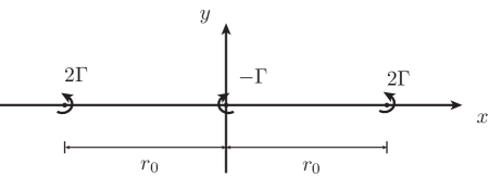
When point vortex equilibria of the 2D Euler equations (inviscid) are used as initial conditions for the corresponding Navier-Stokes equations (viscous), typically an interesting and complex dynamical process unfolds at short and intermediate time scales, which depends crucially on the details of the initial configuration. For long enough times, Gallay & Wayne proved recently that the Lamb-Oseen solution is an asymptotically stable attracting solution for all (integrable) initial vorticity fields [1]. While very powerful, this asymptotic result does not elucidate the intermediate dynamics that take place in finite time and allow a given initial vorticity field to reach the single-peaked Gaussian distribution of the Lamb-Oseen solution. Given the rather large (and growing) literature on point vortex equilibria of the Euler equations, (see for example, [2, 3, 4]), we thought an analysis of how these equilibria evolve under the evolution of the full Navier-Stokes system would merit a systematic treatment. Hence, in this paper, we begin an investigation of the viscous evolution of a class of initial vorticity fields consisting of the superposition of Dirac-delta functions or point vortices [2]. Our initial configuration, shown in Figure 1, is a collinear configuration of three point vortices, evenly spaced along a line (the axis), with strengths , , and , respectively. Such a configuration, for the Euler equations, is known to be an unstable fixed equilibrium, as fleshed out most recently and comprehensively in [5], but earlier in [6]. We point out that this configuration, because of the strengths chosen for each of the point vortices, is not what is commonly referred to as the ‘tripole’ state [7, 8, 9, 10] in which the vortex strengths sum to zero. Our focus in this paper will be the dynamics that takes place at the short and intermediate time scales, using this initial state in the Navier-Stokes equations, before the long-time asymptotic Lamb-Oseen solution dominates. This includes the dynamics of the surrounding passive field and the corresponding background time-dependent streamline pattern in an appropriately chosen reference frame which we argue is very helpful as a diagnostic tool to interpret the resulting flowfield.
2 Problem Setting
Consider an incompressible fluid in an unbounded two-dimensional (2D) domain . The fluid motion is governed by Navier-Stokes equations, written in terms of the vorticity field , a scalar-valued function of position and time , as follows
| (1) |
The kinematic viscosity is assumed to be constant. The fluid velocity is a vector-valued function of and . Both and are expressed in an inertial frame where span the plane of motion, that is to say, one has and or, equivalently, and . By definition, the vorticity vector is always perpendicular to the plane of motion and can thus be expressed as . The velocity and vorticity are related via the 2D Biot-Savart law
| (2) |
where is an integration variable and . Note that for 2D flows, the stretching term is identically zero thus does not appear in (1) while the continuity equation is trivially satisfied when expressed in terms of vorticity.
The solution of the system of equations (1) and (2) depends, of course, on the choice of initial conditions . One solution of particular interest in this work is the well-known Lamb-Oseen solution corresponding to a Dirac-delta initial condition , i.e., a point vortex placed at the origin with circulation or strength (more generally, the circulation around any closed curve in the fluid domain is defined as and can be thought of as the flux of vorticity through the area enclosed by the curve ). Traditionally, the problem can be expressed compactly in complex notation with position variable , and . The Lamb-Oseen solution is given by (see, for example, [11, 2] for more details)
| (3) |
The corresponding velocity field is given by,
| (4) |
where the dot notation refers to the time derivative and the notation refers to the complex conjugate. According to (3), the evolution of a vorticity field that is initially concentrated at the origin is such that the vorticity diffuses axisymmetrically as a Gaussian distribution. The spreading of the vorticity concentration can be quantified by the vortex core or support defined as , where .
Despite the explicit, exact, and simple nature of the solution (3), for more complicated initial data, explicit solutions of (1) and (2) are not analytically available for a general initial vorticity field. We are particularly interested in the viscous evolution of a class of initial vorticity fields consisting of the superposition of Dirac-delta functions or point vortices. Note that Gallay & Wayne proved recently that the Lamb-Oseen solution is an asymptotically stable attracting solution for all (integrable) initial vorticity fields, see [1], of which is a special case. It is the dynamics that unfolds as the system evolves towards this final state that we are interested in.
The dynamics of point vortices in the plane is extensively analyzed in the context of the inviscid fluid model (), see for example [2] and references therein. The vorticity field remains then concentrated for all times at points whose position () is dictated by the local fluid velocity induced by the presence of the other vortices. The fluid velocity at an arbitrary point in the plane that does not coincide with a point vortex is obtained from the Biot-Savart law (2) which takes the form
| (5) |
whereas the velocity at a point vortex is given by subtracting the effect of that point vortex from (5), and replacing with , namely,
| (6) |
The first-order ordinary differential equations (6) dictating the inviscid evolution of point vortices are known to exhibit regular, including fixed and moving equilibria, as well as chaotic dynamics depending on the number of vortices, their strengths and initial positions. The literature on this general topic is large, and we refer simply to the influential 1983 review article of Aref [12], along with the monographs of Saffman [11] (especially Chapter 7) and Newton [2] for an immediate entry into the literature. We also mention the 2008 IUTAM Symposium ‘150 Years of Vortex Dynamics’ held at the Technical University of Denmark in which the lively state-of-the-art developments were reported [13].
In order to highlight the way in which the presence of viscosity affects the inviscid point vortex dynamics, we focus on studying the viscous evolution of point vortices whose location at time correspond to a fixed equilibrium of the inviscid point vortex model (6). For concreteness, we consider the case of collinear and equally-spaced point vortices as shown in Figure 1. Let denote the distance between two adjacent vortices and let be the circulation of the left and right vortices and while be that of the center vortex. Also, let and denote the positions of centers of the left, center and right vortices, respectively. One can readily verify that this configuration constitutes a fixed equilibrium of the inviscid point vortex model (6).
It is convenient to non-dimensionalize the problem using the length scale and the time scale dictated by , namely, . To this end, the non-dimensional parameters are given by
| (7) |
and the non-dimensional variables are of the form
| (8) |
For simplicity, we drop the notation with the understanding that all parameters and variables are non-dimensional hereafter. The Navier-Stokes equation (1) can be rewritten in dimensionless form
| (9) |
where is the dimensionless Reynolds number, here defined as . Some words of caution are in order here, as we will be comparing numerical simulations of the Navier-Stokes equations with our model, and to do so requires that one is able to compare the direct numerical simulation (DNS) Reynolds number with the ‘model’ Reynolds number. For this, it is better to think of the Reynolds number as the ratio of inertial effects over diffusive effects . In some sense, one can think of the term as being primarily responsible for the rotation we will discuss, while the term not only triggers the rotation, but diffuses the cores of the vortices. For any DNS, this creates an ‘effective’ Reynolds number which depends not only on the choice , but also on numerical discretization since it affects the ‘rotation’ and ‘diffusion’. The ‘model’ Reynolds number will be discussed in more detail in the upcoming sections.
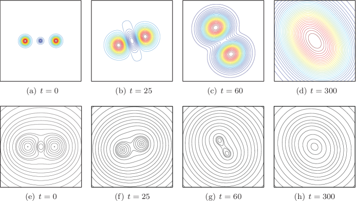
By way of motivation, we first present a numerical solution of the system of equations (9) and (2) subject to the initial condition . We use the numerical algorithm devised in [14] that utilizes a second-order finite difference method with a multi-domain non-reflecting boundary condition to emulate the infinite fluid domain. This is a mesh-based method which poses a problem in handling the Dirac-delta initial conditions because they are not well-posed for discretization on a standard Euclidean mesh. To overcome this problem, we consider the initial conditions of the vorticity field as a superposition of three slightly diffused Gaussian peaks. In all the simulations presented here, we diffuse the initial Dirac-delta vorticity field by such that , e.g., when . This, of course, introduces a slight mismatch in the initial conditions used for the numerical simulation with those used in the model, an error we cannot completely eliminate, but should be kept in mind when comparing the simulation with the model. We compute the time evolution of the vorticity field in the window while the non-reflecting boundary conditions are imposed using the multi-domain technique with 10 nested domains, the largest of which is times the size of our result window. The spatial and time steps are set to , .
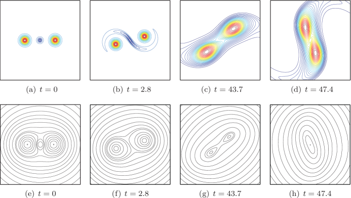
Figure 2 depicts the time evolution of the vorticity contours (top row) and streamlines (bottom row) of Navier-Stokes solution for at four time instants: and . One notices that the vortex configuration begins to rotate unsteadily for ; we refer to this motion as viscosity-induced rotation. One also notices that the center vortex stretches and diffuses out first, then the outer two vortices begin to merge. Eventually the vortex configuration approaches a single Gaussian vortex.
3 The multi-Gaussian model
In this section, we use a simple, analytically-tractable model to describe the dynamic evolution of point vortices for non-zero (but small) viscosity (. The model assumes that the vorticity of each initial point vortex spreads axisymmetrically as an isolated Lamb-Oseen vortex, thus modeling the diffusion term in (1), while its center moves according to the local velocity induced by the presence of the other (diffusing) vortices, thus accounting for the convection term in (1). It is worth noting here the recent work of Gallay [15] who analyses the inviscid limit of the 2D Navier-Stokes evolution of Dirac-delta initial conditions and proves, under certain assumptions, that the solution of the Navier-Stokes equation converges, as , to a superposition of Lamb-Oseen vortices. In this work, we show that, for small yet finite , the multi-Gaussian model is able to capture qualitatively, though not quantitatively, some of the main features of the Navier-Stokes solution. Generally speaking, this class of models has been most highly developed in the numerical literature (see for example [16, 17] and subsequent analysis in [18]) and is referred to as a ‘core-growth’ class of models. One can trace the ‘splitting’ idea of the advection and the diffusion terms of the 2D Navier-Stokes equations, on which the core growth model is based, at least back to Chorin’s influential paper [19], also used by Milinazzo and Saffman [20]. In these papers, the diffusion was handled by a random walk approach. Core growth models based on time-dependent solutions of the heat-equation were developed and used mostly by the numerical/computational vortex dynamics community, and are discussed and developed explicitly in [21, 22, 23, 24]. In the context of numerical simulations, focused studies can be found in the works of Barba and Leonard [25, 26], and used in specific models in [27, 28, 29]. We mention, of course, also the works [30, 31, 1] and the 2009 Ph.D. thesis of Uminsky [32] and follow-up work [33] which develops an eigenfunction expansion method based on the form of the heat-kernel. Additionally, we mention the body of work generated by Dritschel and co-workers, of which [34, 35] would be two relevant examples, whose aim is to elucidate via Lagrangian type numerical simulations, the host of complex processes associated with mixing and dynamics in viscously evolving two-dimensional flows.
The model assumes that the vorticity field at all times is a superposition of multiple Lamb-Oseen vortices
| (10) |
The associated velocity field is computed by substituting (10) into (2)
| (11) |
The velocity at the center of the vortex is given by subtracting the effect of that vortex and replacing by in (11)
| (12) |
The system of equations in (10), (11), and (12) is referred to as the multi-Gaussian model. We emphasize that we include in this model the equation (11) for the evolution of passive tracers in the ‘field’ which is transported under the dynamics generated by (10) and (12). This will be discussed more thoroughly in Section 5 and is relevant for comparisons of panels (a)-(d) of Figure 2 with (a)-(d) of Figure 3.
According to (10), the vorticity field associated with the initial three-vortex configuration shown in Figure 1 is given by
| (13) |
The location of the centers of the vortices , and is obtained by solving the set of six first-order, ordinary differential equations in (12). From symmetry, one can readily verify that and that the centers of the vortices remain collinear and equally-spaced with constant distances for all time. The vorticity contours of (10) are then plotted in Figure 3 (top row). The streamlines associated with the velocity field in (12) is shown in Figure 3 (bottom row). Similarly to the Navier-Stokes solution depicted in Figure 2, the dynamic evolution of the multi-Gaussian model is characterized by: (i) an unsteady rotation of the whole vortex configuration for , (ii) a stretching of the middle vortex, and (iii) eventual merging of the outer two vortices to form one single-peaked Gaussian of strength as shown in Figure 3. However, here some care is in order, as clearly Figures 2(b)-(d) (DNS) and Figures 3(b)-(d) show some important differences. Not only are the timescales different, but Figure 2(b) shows a convective ‘wrappping’ and ‘stretching’ of the middle vortex around the outer two before the diffusive effects kick in, whereas Figure 3(b) shows the stretching, but not the wrapping. Here it is important to remember that the passively advected field, as shown in Figure 13, is an important part of the model, and this field does show some of the same nonlinear wrapping features that appear in the DNS Figure 2(b). One could say, in some respects, that the outer two vortices, being twice the strength of the inner one, are the primary ‘drivers’ of the flowfield, which is perhaps why Figure 2(e)-(h) match relatively well with Figure 3(e)-(h). The ‘passively advected’ inner vortex shown in Figure 2(b) is better reflected in the passive particle field shown in Figure 13 and discussed at length in Section 5. In turn, because the passively advected field in our model is not affecting the vorticity evolution, whereas in the DNS it is, this helps explain why the timescales associated with the two are different. The model is not an exact solution of the Navier-Stokes equations, and this appears to be the main physical manifestation of this fact.
The unsteady rotation rate of the vortex structure is obtained analytically as follows. From (12), the velocity of one of the outer vortices, say the right vortex, takes the form
| (14) |
Now, by symmetry one has , and , where is the angle between the line traced by the vortex centers and the axis, and . One gets, upon substituting into (14) and simplifying, that the rotation rate is given by
| (15) |
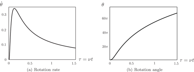
In Figure 4 is a depiction of versus which shows that the rotation rate starts from zero, reaches a maximum value at an intermediate time and eventually decays to zero as . The values of and are given by
| (16) |
The orientation angle can be readily obtained by integrating (15) in time
| (17) |
where the exponential integral is defined as in the sense of principle value, which can be evaluated numerically to machine accuracy.
It is convenient for analyzing the flow to express the fluid velocity field in a frame co-rotating with the vortex configuration at the time-dependent rotation . Let denote position of a point in the plane expressed in the rotating frame. The point transformation from the rotating to the inertial frame is given by
| (18) |
The fluid velocity transforms as where is the velocity field expressed in the rotating frame. In component form, equations (11) transform as
| (19) |
and
| (20) |
where we used .
The instantaneous stagnation points of the velocity field (obtained by setting the right-hand side of (19), (20) to zero) reveal important information about the instantaneous streamlines of the fluid velocity field. From symmetry of the velocity field, the instantaneous stagnation points must lie on the and axes. One finds a total of five fixed points: one initially elliptic point at the origin, a pair of initially hyperbolic points at and a pair of initially elliptic points at . The hyperbolic and elliptic character of these stagnation points is obtained by linearizing (19) ,(20) about the instantaneous stagnation points and computing the eigenvalues of the linearized system. A pair of eigenvalues is associated with each stagnation point. One has a hyperbolic point if is real and an elliptic point if is pure imaginary.
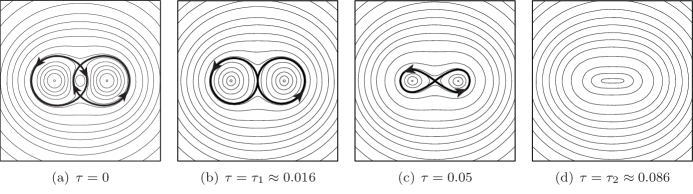
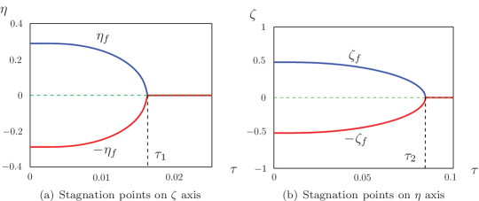
At time , the streamlines are those of the inviscid equilibrium, with a separatrix linking the two hyperbolic stagnations points on the axis, as shown in Figure 5. Initially, the separatrix divides the fluid domain into four regions: three regions, one around each point vortex or elliptic point, and a fourth region bounded by the separatrix and the bound at infinity and void of point vortices. As time evolves, the location of the instantaneous stagnation points change as shown in Figure 5, and the separatrix evolves accordingly. Note that the time-dependent separatrix does not constitute barriers to fluid motion and fluid particles typically move across this separatrix as time evolves as discussed in more details in Section 5. Figure 6 shows the coordinates of the stagnation points and as functions of time. The pair of initially hyperbolic points start from then collide together with the elliptic point at the origin in finite time to transform the origin into a hyperbolic point. This collision of instantaneous stagnation points is accompanied by a change in the streamline topology where the region around the center vortex disappears, see Figure 5. Time is referred to as the first bifurcation time. (Note that the first bifurcation time does not correspond to when the cores of the three Gaussian vortices touch for the first time which takes place at , nor does it correspond to when the cores of the two outer Gaussian vortices touch . Indeed, the definition of core size of a Gaussian function is rather ad hoc and bears little relevance to the dynamics of the multi-Gaussian model.) Similarly, starts from and collides at the now hyperbolic point at the origin at time . Time is referred to as the second bifurcation time. For , one has one single elliptic point at the origin as expected from the asymptotic Lamb-Oseen solution.
4 Comparison to Navier-Stokes
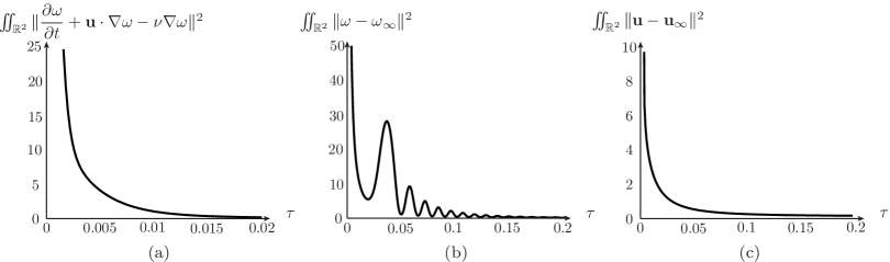
The residual of the model is computed by substituting the solution of (10) and (11) into the Navier-Stokes equation (9). If the solution of the model is also an exact solution of the Navier-Stokes equation for a given set of initial conditions, the residual is identically . In general, is not zero (see discussions of this in [21]) and it can be viewed as an indication of the inaccuracy of the multi-Gaussian model. The norm of residual is plotted as a function of time in Figure 7(a) for the collinear vortex configuration considered here. Figure 7(a) shows that as increases, the norm of tends to zero, indicating that the multi-Gaussian model agrees with the Navier-Stokes solution for large. From the result of Gallay & Wayne [1] and since the total circulation of the initial vorticity field is , we know as the Navier-Stokes solution approaches a single Gaussian vorticity distribution centered at the origin with circulation . We compute the difference between the multi-Gaussian model and this asymptotic solution . Figure 7(b) and (c) show the norm of the difference in both vorticity and velocity, respectively. These plots confirm that the multi-Gaussian model approaches the asymptotic Lamb-Oseen solution for large time but at the intermediate times, the multi-Gaussian model exhibits richer dynamics than the asymptotic Lamb-Oseen solution. While the dynamics of the multi-Gaussian model at these intermediate time scales does not faithfully track the Navier-Stokes solution (as seen from Figure 7(a)), it does capture more details than the asymptotic Lamb-Oseen vortex and its evolution seems to exhibit the main qualitative features of the Navier-Stokes model as argued next.
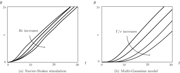
It is evident from Figures 2 and 3 that both the Navier-Stokes equations and the multi-Gaussian model exhibit a viscosity-induced rotation as . In Figure 8 we compare the qualitative trends of rotation angle obtained from the numerical solution to the Navier-Stokes equation and the analytical solution of multi-Gaussian model. In the Navier-Stokes solution, the rotation angle is obtained by computing the angle between the line traced by the vorticity peaks (see Figure 2) and the axis while it is given by (17) in the multi-Gaussian model. Clearly, both the Navier-Stokes solution and the model, although quantitatively distinct, exhibit similar qualitative trends in that the rotation angle is smaller when increases (in Navier-Stokes) or equivalently when increases (in the model). As cautioned earlier about comparing DNS Reynolds numbers with the ‘model’ Reynolds number, if both are thought of strictly as , we can only claim qualitative overlap with the model and DNS. To obtain more quantitative overlap would require more effort on our part to obtain an accurate Lagrangian based DNS to get a more detailed handle on the effective ‘numerical’ Reynolds number, along with a modified model system that does more to couple rotational effects with diffusive effects, neither of which are the immediate goals of the current work.
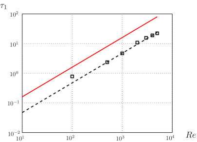
To quantify the difference between the Navier-Stokes solution and the multi-Gaussian model, we focus on comparing the first bifurcation time in the Navier-Stokes simulation for different to the first bifurcation time in the model. The result is plotted in Log-Log scale in Figure 9 for and (plotted in squares). The dashed line is the best fitted straight line using the least square distance rule. The fitted line can be expressed as , which means in linear scale, the fitting is . The simulation results are compared to the first bifurcation time as predicted by the multi-Gaussian model. While the first bifurcation in the simulations happens earlier than in the model, both the Navier-Stokes simulations and model indicate that is linearly dependent on (or ).
5 Evolution of vorticity in the multi-Gaussian model
We now use the multi-Gaussian model to analyze the fluid velocity and vorticity fields at intermediate time scales before the asymptotic state of a single Lamb-Oseen vortex dominates. The goal of this analysis is to understand the intermediate mechanisms that lead the initial point vortex configuration to reach the asymptotic Lamb-Oseen vortex.
As time evolves, the vorticity field, initially concentrated at and , begins to spread spatially inducing a velocity field similar to that of a Rankine vortex with time-dependent core. By way of background, the reader is reminded that the fluid velocity at a point associated with a Rankine vortex at the origin with vorticity (corresponding to the total circulation of the collinear vortex structure) is perpendicular to the distance from the origin and its value is given by
| (21) |
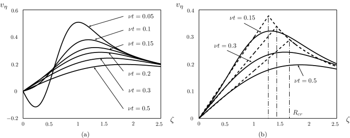
The value is referred to as the core of the Rankine vortex. For , the fluid velocity corresponds to a rigid rotation while for , the velocity field decays proportionally to the inverse of the distance . As time evolves, the velocity field induced by the viscously evolving collinear vortex structure becomes analogous to that of a Rankine vortex with vorticity and time-dependent core, as seen in Figures 10. This analogy is especially evident in Figures 10(b) where we superimpose the velocity field of the Rankine vortex on that induced by the viscously evolving collinear vortex structure at three different instances. Close to the origin, the velocity field of the collinear vortex structure looks like a rigid rotation, and the rotation rate is given by in (15). Since the rotation rate is unsteady, the core size of the Rankine vortex, obtained by equating , is time dependent and it increases with time as shown in Figures 10(a). As the distance from the origin increases, the velocity field of the collinear vortex structure decays analogously to the inverse decay with vorticity .
Motivated by this analogy with the Rankine vortex, we examine the time evolution of the relative velocity field
| (22) |
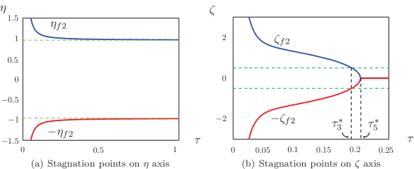
obtained by subtracting a rigid body rotation from the fluid velocity field expressed in the rotating frame (written in (19), (20) in component form). Similarly to the analysis in Section 3, we identify the instantaneous stagnation points associated with the relative velocity field (22). Immediately as increases from zero (), in addition to the elliptic stagnation points located at the origin and and the hyperbolic points at , one gets two new pairs of stagnation points appearing from infinity: one elliptic pair located at and one hyperbolic pair located at . Figure 11(a) shows the values of as functions of time. Clearly, start from and eventually converge to final values . The pair remains elliptic for all time. Figure 11(b) shows that the pair also starts from and reaches at then the origin at . Meanwhile, the topology of the streamlines of the relative velocity field changes as a result of five distinct bifurcations as depicted in Figure 12 and explained next, thus the notation .
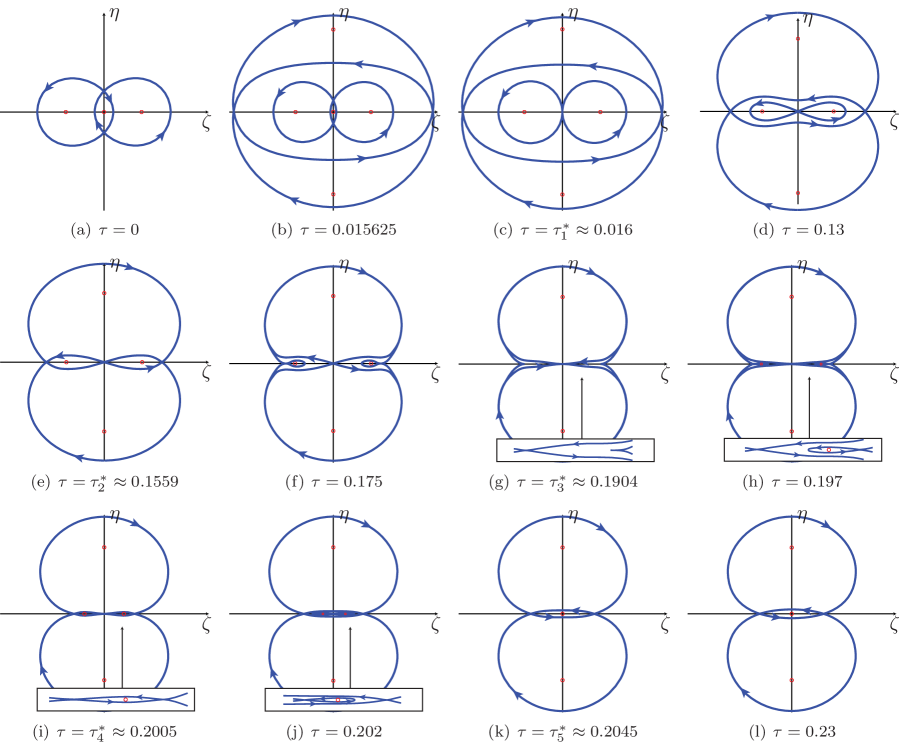
The first bifurcation in the streamline topology is due to the same mechanism explained in Section 3 and takes place at the same time , see Figure 12(c). The second bifurcation does not coincide in time with the second bifurcation identified in Section 3, that is, . It is associated with a change in the streamline topology caused by a collapse of the separatrices associated with the hyperbolic pair onto the separatrices of the now hyperbolic point at the origin, see Figure 12(e). The third bifurcation occurs at when the hyperbolic points at collide with the elliptic points at , respectively, causing them to change to hyperbolic points, see Figure 12(g). After the third bifurcation, one still has two pairs and of stagnation points on the -axis but with exchanged hyperbolic/elliptic characters. The fourth bifurcation takes place at due yet to another collapse of the separatrices of the hyperbolic point at the origin with the separatrices at the now hyperbolic points at , see Figure 12(i). The fifth bifurcation takes place at when the now elliptic pair collides with the hyperbolic origin causing it to turn into an elliptic point, see Figure 12(k). This bifurcation sequence turns out to be crucial in dictating the time evolution of the vorticity field which we visualize using colored passive tracers as commonly done in experimental and computational fluid mechanics (see, for example, [9]).
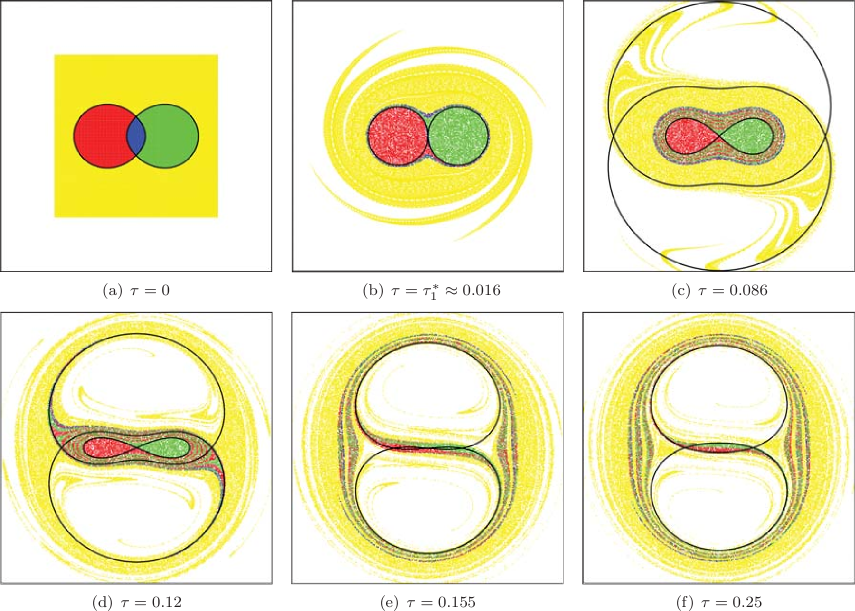
We seed the flow at time with passive tracers of four different colors as shown in Figure 13(a) to distinguish the initial four fluid regions identified in Section 3, namely, the three regions around the vortices bounded by the separatrix (seeded with red, blue and green particles, respectively) and the fourth region (seeded with yellow particles) bounded by the separatrix and the bound at infinity. We let the passive tracers be advected by the fluid velocity field given in (11). Snapshots of the passive tracers at six distinct instants in time are depicted in Figure 13. As time evolves, the location of the stagnation points and the associated separatrices change. Due to incompressibility, the particles initially in the region around the middle vortex (blue color) ‘leak’ along the unstable branch of separatrices associated with the instantaneous hyperbolic points . At , Figure 13(b) shows that all the particles are squeezed out of the middle region. Meanwhile as time progresses, the fluid particles in yellow begin to form lobes that stretch at a finite distance away from the initial location of the vortices, see Figure 13(c). Qualitatively, the passive tracers in Figure 13(c) indicate a vorticity field similar to that obtained from the Navier-Stokes simulation in Figure 2(d) (modulo the rigid rotation of the whole structure). The formation of these lobes cannot be explained based on the analysis of the streamline patterns in Section 3. Indeed, the formation of these lobes is initiated when the yellow passive tracers encounter the separatrices associated with the hyperbolic points of the relative velocity field (22) that appear from infinity and move towards the origin along the -axis (see Figure 11(b)). The lobes then stretch and rotate around the elliptic points that appear from infinity and converge to a finite distance away from the origin (see Figure 11(a)). Eventually, the passive particles initially placed in the regions around the point vortices, whose detailed evolution is also dictated by the sequence of bifurfactions described in Figure 12, join the large lobes as well and begin to stretch and rotate at a finite distance away from the initial vortex configuration, see Figure 13(d)–(f). After the last bifurcation in Figure 12(k), all the passive particles continue to rotate as shown in Figure 13(f). We emphasize that this interesting dynamics of the passive particles, which in turn indicates the evolution of the vorticity field, cannot be explained based solely on the analysis of the streamlines of the fluid velocity field of Section 3. In addition, because of the detailed and delicate nature of the full series of topological bifurcations that occur, to capture all but the first of these in a DNS would require considerable further effort and is beyond the scope of the current manuscript.
6 Conclusions
The redistribution (inviscid) and diffusion (viscous) of delta-function initial distributions of vorticity, although configuration independent for sufficiently long timescales, is highly dependent on the initial positions and strengths of the point vortices on short and intermediate timescales. These are typically the timescales in which much of the important mixing, transport, and redistribution of vorticity is achieved in many settings. Greengard’s 1985 paper notwithstanding [21] pointing out that the types of models based on advection and core diffusion are not exact solutions of the Navier-Stokes equations, these ideas are exceptionally useful in getting a handle on some of the important dynamical mechanisms that occur during the evolution towards the ultimate Lamb-Oseen state. In fact, one contribution of the current manuscript is to further quantify and understand the limitations of ‘core-growth’ type models as diagnostic tools for understanding more and more complex flows and to point out some of the delicate issues in comparing a DNS with these models. Not surprisingly, core-growth type models are also useful as starting points for more sophisticated numerical methods which systematically exploit some of the main features [16, 24] (Also, see Blobflow, an open source vortex method package developed by Rossi, available at http://www.math.udel.edu/rossi/BlobFlow as of October 2010).
We summarize here with three main points associated with the viscous evolution of the three-vortex collinear state whose initial configuration corresponds to an unstable inviscid fixed equilibrium:
(i) The presence of viscosity immediately ‘triggers’ the underlying instability of the equilibrium, causing the vortices to rotate unsteadily;
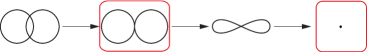
(ii) In a fixed frame of reference, as the system evolves towards the ultimate Lamb-Oseen solution, the streamline patterns associated with the velocity field undergo a clear sequence of topological bifurcations which we depict in Figure 14. We show the ‘homotopic equivalence’ of each of the distinct patterns in the panels - the time and quantitative values of the pattern are not depicted, just the sequence of distinct patterns that appear during the time sequence;
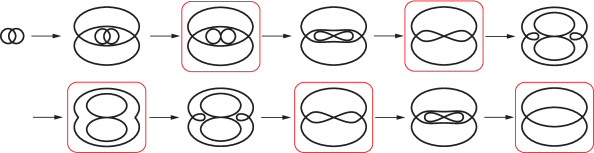
(iii) More interestingly, since the velocity field near the origin is of approximate solid-body (Rankine) form, if we subtract off this field and re-plot the homotopic sequence of patterns that emerges, shown in Figure 15, a far richer and more instructive sequence of patterns is revealed, one that is far more relevant for the understanding of the evolution of passive particle transport, as shown clearly in Figure 13.
We finish by mentioning connections of this work in two other contexts. First, there is by now a growing body of work on calculating ‘time-dependent separatrices’ in developing flows that goes under the name of ‘Lagrangian coherent structures’ (LCS) [37, 38]. Certainly these tools are potentially useful for further elucidating the intermediate timescale dynamics associated with the evolution towards the Lamb-Oseen state, particularly for more complex initial patterns that perhaps start out as relative equilibria of the Euler equations. Second, if one regards, the vorticity field as a probability density function associated, for example, with the positions of initial system of point vortices undergoing a random walk, there are meaningful interpretations of the models used in this paper that have been discussed most recently, for example, in [39, 40, 41]. While this interpretation has not been the main focus of our work, we do find it potentially ripe for future development.
Acknowledgments.
This work is partially supported by the National Science Foundation through the CAREER award CMMI 06-44925 (FJ and EK) and the Grant NSF-DMS-0804629 (PKN).
References
- [1] Gallay, T., Wayne, C.E., [2005], Global Stability of Vortex Solutions of the Two-dimensional Navier-Stokes Equation, Comm. Math. Phys., 255(1), 97-129.
- [2] Newton, P.K., [2001], The N-Vortex Problem: Analytical Techniques, Applied Mathematical Sciences Vol. 145, Springer-Verlag, New York.
- [3] Aref, H., Newton, P.K., Stremler, M., Tokieda, T., Vainchtein, D.L., [2002], Vortex crystals, Adv.. Appl. Mech., 39 1-79.