Sunyaev–Zel’dovich observations of galaxy clusters out to the virial radius with the Arcminute Microkelvin Imager

Abstract

We present observations using the Small Array of the Arcminute Microkelvin Imager (AMI; 14–18 GHz) of four Abell and three MACS clusters spanning 0.171–0.686 in redshift. We detect Sunyaev-Zel’dovich (SZ) signals in five of these without any attempt at source subtraction, although strong source contamination is present. With radio-source measurements from high-resolution observations, and under the assumptions of spherical $\beta$-model, isothermality and hydrostatic equilibrium, a Bayesian analysis of the data in the visibility plane detects extended SZ decrements in all seven clusters over and above receiver noise, radio sources and primary CMB imprints. Bayesian evidence ratios range from $10^{11}$:1 to $10^{43}$:1 for six of the clusters and 3000:1 for one with substantially less data than the others. We present posterior probability distributions for, e.g., total mass and gas fraction averaged over radii internal to which the mean overdensity is 1000, 500 and 200, $r_{200}$ being the virial radius. Reaching $r_{200}$ involves some extrapolation for the nearer clusters but not for the more-distant ones. We find that our estimates of gas fraction are low (compared with most in the literature) and decrease with increasing radius. These results appear to be consistent with the notion that gas temperature in fact falls with distance (away from near the cluster centre) out to the virial radius.

1 Introduction

The Sunyaev–Zel’dovich (SZ) effect (Sunyaev & Zeldovich, 1970, 1972) is the inverse-Compton scattering of the CMB radiation by hot, ionised gas in the gravitational potential well of a cluster of galaxies; for reviews see Birkinshaw (1999) and Carlstrom et al. (2002). The effect is useful in a number of ways for the study of galaxy clusters; here we are concerned with two in particular. First, because the SZ effect arises from a scattering process, a cluster at one redshift will produce the same observed SZ surface brightness as an identical cluster at any other redshift, so that the usual sensitivity issue of high-redshift observing does not arise. Second, since the SZ surface brightness is proportional to the line-of-sight integral of pressure through the cluster, the SZ signal is less sensitive to concentration than the X-ray Bremmsstrahlung signal; one corollary of this is that the ratio SZ-sensitivity / X-ray-sensitivity increases with distance from the cluster centre so that with SZ one can probe out to, say, the virial radius, provided the SZ telescope is sensitive to sufficiently large angular scales.

SZ decrements are faint, however, and can be contaminated or obliterated by other sources of radio emission. A range of new, sensitive instruments has been brought into use to capitalise on the science from SZ observations. Among these instruments, which employ different strategies to maximise sensitivity and minimise confusion, are ACT (Swetz et al., 2010; Menanteau et al., 2010), AMI (AMI Consortium: Zwart et al., 2008) AMiBA (Ho et al., 2009; Wu et al., 2009), APEX (Dobbs et al., 2006), CARMA (www.mmarray.org), SPT (Carlstrom et al., 2009; Andersson et al., 2010) and SZA (Culverhouse et al., 2010). In the case of AMI, two separate interferometer arrays are used, the Small Array (SA) having short baselines sensitive to SZ and radio sources, and the Large Array (LA) with baselines sensitive to the radio sources alone and thus providing source subtraction for the SA. Key parameters of the SA and LA are shown in Table 1.

The SA was built first. Partly to test it while the LA was being completed, we used the SA to observe Galactic supernova remnants and likely regions of spinning dust (AMI Consortium: Scaife et al. 2008, AMI Consortium: Scaife et al. 2009a,b, AMI Consortium: Hurley-Walker et al. 2009a,b) bright enough not to need source subtraction. But we also wanted to begin SZ observation, test our algorithms to extract SZ signals in the presence of radio sources, CMB primary anisotropies and receiver noise, and begin our SZ science programme. To do this required the use of long-baseline data from the 15-GHz Ryle Telescope (RT; see e.g. Grainge et al. 1993, Grainge et al. 1996, Grainge et al. 2002a,b, Cotter et al. 2002a,b, Grainger et al. 2002, Saunders et al. 2003, Jones et al. 2005) taken in the past; this needs caution because of radio source variability (see e.g. Bolton et al. 2006, Sadler et al. 2006 and AMI Consortium: Franzen et al. 2009), but our data-analysis algorithm allows for variability and in fact we were able to use some data from the LA, which, at the time, was only partially commissioned. Here we present the first part of this work, SZ measurements of seven known clusters spanning ranges of redshift $z$ and of X-ray luminosity $L_{X}$.

We assume a concordance $\Lambda$CDM cosmology, with $\Omega_{\mathrm{m}}=0.3$, $\Omega_{\Lambda}=0.7$ and $H_{0}=70\;\mathrm{km}\;\mathrm{s}^{-1}\;\mathrm{Mpc}^{-1}$. However, in plots of probability distribution, we explicitly include the dimensionless Hubble parameter, defined as $h~{}\equiv~{}H_{0}/\left(100\,\mathrm{kms}^{-1}~{}\mathrm{Mpc}^{-1}\right)$, to allow comparison with other work. All coordinates are J2000 epoch. Our convention for spectral index $\alpha$ is $S_{\nu}\propto\nu^{-\alpha}$ where $S$ is flux density and $\nu$ is frequency. We write the radius internal to which the average density is $a$ times the critical density $\rho_{\mathrm{crit}}$ at the particular redshift as $r_{a}$, the total mass (gas plus dark matter) internal to $r_{a}$ as $M_{a}$, and the gas mass internal to $r_{a}$ as $M_{\mathrm{gas},a}$.

Table 1: AMI (AMI Consortium: Zwart et al., 2008) technical summary.

	SA	LA
Antenna diameter	3.7 m	12.8 m
Number of antennas	10	8
Baseline lengths (current)	5–20 m	18–110 m
Primary beam (15.7 GHz)	$20\aas@@fstack{\prime}1$	$5\aas@@fstack{\prime}5$
Synthesized beam	$\approx 3\arcmin$	$\approx 30\arcsec$
Flux sensitivity	30 mJy s1/2	3 mJy s1/2
Observing frequency	13.9–18.2 GHz
Bandwidth	4.3 GHz
Number of channels	6
Channel bandwidth	0.72 GHz

2 Cluster selection and RT observation

We used the NOrthern ROSAT All-Sky Survey (NORAS, Böhringer et al. 2000) catalogue as a source of low-redshift ($z<0.3$) clusters, and the MAssive Cluster Survey (MACS, Ebeling et al. 2001, Ebeling et al. 2007, Ebeling et al. 2010) to give secure, more-distant clusters that provide some filling-out of the $L_{X}$–$z$ plane. We restricted redshifts to $z>0.1$ to avoid resolving out SZ signals, and luminosity to $L_{\mathrm{X}}>7\times 10^{37}$ W ($0.1$–$2.4$ keV, rest frame).

We restricted declinations to greater than $20\degr$ since the RT had only East-West baselines, and further excluded clusters which we knew, from the NVSS (Condon et al., 1998) or from archival RT data, would be too contaminated by radio sources. Details of the resulting seven clusters in this work are given in Table 2. Source surveying of the remaining clusters with the compact array of the RT – note that this array contained five of the eight antennas of the LA – was then carried out as follows.

The RT data were obtained between 2004 and 2006. Each cluster field was surveyed in two ways: with a wide shallow raster and a deep central one. The wide shallow raster comprised a hexagonal close-packed raster of $11\times 12$ pointings on a $5\arcmin$ grid, with a dwell time at each pointing of eight minutes; the aim was to identify relatively bright radio sources in the direction of an SA pointing. The centre of each cluster was followed up with a hexagon of $7\times 12$-hour RT pointings, on a $5\arcmin$ grid, in order to detect faint sources near the target cluster.

Data were reduced, and point-source positions and fluxes extracted, using procedures developed for the 9C survey and outlined in Waldram et al. (2003). The source data are given in Table 3.

Table 2: Clusters in this work. Temperatures, redshifts and X-ray luminosities are from ¹LaRoque et al. (2006), ² Balestra et al. (2007) ³ Bonamente et al. (2008) ⁴ Ebeling et al. (2007), ⁵Böhringer et al. (2000), ⁶Struble & Rood (1999), ⁷ Ebeling (Priv. Comm.). The map noise indicated is for a SA naturally-weighted map with all baselines and no source subtraction. The integration times $t_{\mathrm{int}}$ are on-sky times, and do not account for variations in system temperature with airmass or poor weather, or for the amount of data flagged due to, for example, shadowing.

Cluster	RA (J2000)	Dec (J2000)	$z$	$T_{\mathrm{e}}$/keV	$L_{X}/10^{37}$W	$t_{\mathrm{int}}$/hours	$\mathrm{rms}$/$\mu$Jy
A611	08 00 59.40	+36 03 01.0	0.288 (5)	$6.79^{+0.41}_{-0.38}\,(1)$	8.63 (5)	23.8	140
A773	09 17 52.97	+51 43 55.5	0.217 (6)	$8.16^{+0.56}_{-0.52}\,(1)$	12.11 (5)	23.8	160
A1914	14 26 02.15	+37 50 05.8	0.171 (5)	$9.48^{+0.35}_{-0.29}\,(1)$	15.91 (5)	20.9	140
A2218	16 35 52.80	+66 12 50.0	0.171 (5)	$7.80^{+0.41}_{-0.37}\,(1)$	8.16 (5?)	62.4	90
MACSJ0308+26	03 08 55.40	+26 45 39.0 (7)	0.352 (7)	$11.2^{+0.7}_{-0.7}\,(2)$	15.89 (7)	86.6	140
MACSJ0717+37	07 17 30.00	+37 45 00.0 (7)	0.545 (4)	$11.6^{+0.5}_{-0.5}\,(4)$	25.33 (7)	23.8	160
MACSJ0744+39	07 44 48.00	+39 27 00.0 (7)	0.686 (4)	$8.14^{+0.80}_{-0.72}\,(1)$	17.16 (7)	71.8	320

Table 3: Contaminating sources. W denotes RT wide, shallow raster ($11\times 12$ pointings), while H denotes a RT deep hexagon (7 pointings). Fluxes from RT shallow raster observations were boosted by 10 per cent to account for pointing errors (Waldram et al., 2003). 9C denotes data from 9C pointed observations (Waldram et al., 2003), with the flux error estimated at $<5$ per cent.

Cluster		RA (J2000)	Dec (J2000)	Array	Mode	S/mJy
A611	1	08 00 43.28	+36 14 00.9	SA		$5.5\pm 1.7$
	2	08 00 09.91	+36 04 15.4	SA		$4.4\pm 1.3$
A773	1	09 18 38.29	+51 50 25.0	SA		$4.4\pm 0.4$
	2	09 17 06.13	+51 44 54.9	SA		$3.4\pm 0.3$
	3	09 17 57.02	+51 45 08.0	LA		$0.12\pm 0.01$
	4	09 18 01.33	+51 44 13.1	LA		$0.32\pm 0.03$
	5	09 17 45.31	+51 43 04.6	LA		$0.22\pm 0.02$
	6	09 17 55.58	+51 43 01.1	LA		$0.19\pm 0.02$
	7	09 17 50.67	+51 41 06.1	LA		$0.31\pm 0.03$
A1914	1	14 25 10.21 (SA)	+37 52 35.1 (SA)	SA/LA		$4.2\pm 0.4$ (LA)
	2	14 27 24.75 (RT)	+37 46 33.8 (RT)	RT/LA		$9.7\pm 1.0$ (LA)
	3	14 25 48.02	+37 47 50.3	LA		$1.0\pm 0.3$
	4	14 25 40.84	+37 45 50.4	LA		$3.7\pm 0.4$
	5	14 25 50.53	+37 45 10.3	LA		$0.61\pm 0.18$
	6	14 25 58.53	+37 44 00.1	LA		$0.60\pm 0.18$
	(7)	14 25 50.53	+37 45 10.3	SA		$4.3\pm 1.3$
A2218	1	16 35 47.24	+66 14 46.9	RT	H	$1.9\pm 0.6$
	2	16 36 15.74	+66 14 27.0	RT	H	$1.9\pm 0.6$
	3	16 35 22.14	+66 13 20.6	RT	W	$5.6\pm 1.7$
	4	16 33 18.18	+66 00 50.6	RT	W	$10\pm 3$
	5	16 35 39.78	+65 58 12.0	RT	W	$11\pm 3$
	6	16 34 46.36	+65 55 18.6	RT	W	$13\pm 4$
	7	16 37 22.56	+66 21 18.4	SA(L)		$5.2\pm 1.6$
MACSJ0308+26	1	03 09 42.02	+26 56 30.3	9C	W	$8\pm 2$
	2	03 08 56.52	+26 44 54.0	SA(L)		$2.4\pm 0.7$
	3	03 09 40.14	+26 37 23.6	SA(L)		$2.9\pm 0.9$
MACSJ0717+37	1	07 17 36.09	+37 45 56.3	RT	H	$2.1\pm 0.3$
	2	07 17 35.91	+37 45 11.2	RT	H	$1.8\pm 0.5$
	3	07 17 37.14	+37 44 23.1	RT	H	$3.9\pm 1.2$
	4	07 17 41.06	+37 43 15.2	RT	H	$2.5\pm 0.8$
	5	07 18 10.51	+37 49 14.6	SA(L)		$18\pm 6$
	6	07 16 35.69	+37 39 14.2	SA(L)		$4.7\pm 1.4$
MACSJ0744+39	1	07 44 32.95	+39 32 15.0	RT	H	$2.8\pm 0.2$
	2	07 44 22.30	+39 25 46.5	RT	H	$1.1\pm 0.2$
	3	07 43 58.76	+39 15 02.3	RT	W	$52.0\pm 1.7$
	4	07 43 45.99	+39 14 21.5	RT	W	$8.3\pm 1.7$

3 AMI observation and reduction

The seven clusters were observed with the SA between 2007 October and 2008 January. Each cluster typically had 25 hours of SA observing on the sky (though A2218, MACSJ0308+26 and MACSJ0717+27 had some 70 hours). The uv-coverage is well-filled (Figure 1) all the way down to ${\approx}180{\lambda}$, corresponding to a maximum angular scale of $\approx 10\arcmin$. This is a significantly greater angular scale than is achievable with OVRO/BIMA, the RT, or the SZA.

Calibration and reduction procedures were as follows. One of our two absolute flux calibrators, 3C286 and 3C48, was observed immediately before or after each cluster observation. The absolute flux calibration is accurate to 5 per cent (see AMI Consortium: Hurley-Walker et al. 2009b). Each cluster observation was reduced separately using our in-house software reduce. An automatic reduction pipeline is in place, but all the data were examined by eye for problems. Data were flagged for shadowing, slow fringe rates, path-compensator delay errors and pointing errors. The data were flux-calibrated, Fourier transformed and fringe-rotated to the pointing centre. Further amplitude cuts were made in order to remove interference spikes and discrepant baselines. The amplitudes of the visibilities were corrected for variations in the system temperature with airmass, cloud and weather, and the data weights converted into Jy^-2. Secondary (interleaved) calibration was applied, by observing a point-source calibrator every hour, to correct for system phase drifts. The data were smoothed from one-second to 10-second samples, and calibrated uvfits were outputted and co-added using pyfits. Typically 20–30 per cent of the data were discarded due to bad weather, telescope downtime and other flagging. The data were mapped in aips and also directly analysed in the visibility plane.

In some cases, as indicated in Table 3, it was possible to use some of the then partially commissioned LA for source subtraction, assisting with any effects of the time gap between RT and SA observations (LA calibration and reduction are very similar to that of the SA, described above). Similarly, for some sources of high flux density away from the cluster, the long baselines of the SA provided useful measurements.

3.1 Maps

We used standard aips tasks to produce naturally weighted SA maps with all baselines, no taper and no source subtraction. These images, after cleaning, are shown in Figure 2. The maps have differing noises due largely to differing integration times. Sources are evident in all the maps. In five of the maps, an extended SZ decrement is visible, despite major source contamination at the X-ray centres in the cases of A2218 and MACSJ0308+26. In MACSJ0717+37, there seems to be some negative signal but the source contamination at the map centre is severe (Edge et al., 2003; Ebeling et al., 2004). In MACSJ0744+39, the contamination is less but there is still only a weak decrement – but we note that the thermal noise is at least twice that of every other map.

Subsequent analysis was carried out in the visibility plane, taking into account radio sources, receiver noise and primary CMB contamination, as we describe in the next section.

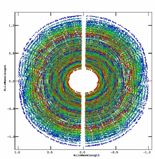
Figure 1: SA uv-coverage for A2218; coverages for the other clusters are very similar to this. The different colours correspond to different frequency channels.

4 Resume of analysis

4.1 Bayesian analysis

Bayesian analysis of interferometer observations of clusters in SZ has been discussed by us previously in e.g. Hobson & Maisinger (2002), Marshall et al. (2003) and Feroz et al. (2009). The advantages of this approach are as follows.

• One infers the quantity that one actually wants, the probability distribution of the values of parameters $\mathbf{\Theta}$, given the data $\mathrm{\mathbf{D}}$ and some model, or hypothesis, $H$, via Bayes’ theorem:

  $$\mathrm{Pr}\left(\mathbf{\Theta}|\mathrm{\mathbf{D}},H\right)=\frac{\mathrm{Pr}\left(\mathrm{\mathbf{D}}|\mathbf{\Theta},H\right)\mathrm{Pr}\left(\mathbf{\Theta}|H\right)}{\mathrm{Pr}\left(\mathrm{\mathbf{D}}|H\right)}.$$ (1)

• The likelihood $\mathrm{Pr}\left(\mathrm{\mathbf{D}}|\mathbf{\Theta},H\right)$ is the probability of the data given parameter values and a model, and encodes the constraints imposed by the observations. It includes information about noise arising from the receivers, primary CMB and unsubtracted radio sources lying below the detection level of the source-subtraction procedure.

• The prior $\mathrm{Pr}\left(\mathbf{\Theta}|H\right)$ allows one to incorporate prior knowledge of the parameter values and, for example, allows one to deal fully and objectively with the contaminants such as sources (which may be variable).

• The evidence $\mathrm{Pr}\left(\mathrm{\mathbf{D}}|H\right)$ is obtained by integrating $\mathrm{Pr}\left(\mathrm{\mathbf{D}}|\mathbf{\Theta},H\right)\mathrm{Pr}\left(\mathbf{\Theta}|H\right)$ over all $\mathbf{\Theta}$, allowing normalization of the posterior $\mathrm{Pr}\left(\mathbf{\Theta}|\mathrm{\mathbf{D}},H\right)$. One can select different models by comparing their evidences, the process automatically incorporating Occam’s razor.

• However, performing these integrations, and sampling the parameter space, is non-trivial and can be slow. The use of the ‘nested sampler’ algorithm MultiNest both speeds up the sampling process significantly and, more importantly, allows one to sample from probability distributions with multiple peaks and/or large curving degeneracies (Feroz & Hobson, 2008).

• Throughout the whole analysis, probability distributions – with their asymmetries, skirts, multiple peaks and whatever else – are used and combined correctly, rather than discarding information (and, in general, introducing bias) by representing distributions by a mean value and an uncertainty expressed only in terms of a covariance matrix.

4.2 Physical Model and Assumptions

We restrict ourselves to the simplest model, by assuming a spherical $\beta$-model for isothermal (see section 4.3), ideal cluster gas in hydrostatic equilibrium. Following e.g. Grego et al. (2001), the equation of hydrostatic equilibrium for a spherical shell of gas of density $\rho$ at pressure $p$, a radius $r$ from the cluster centre is

$$\frac{\mathrm{d}p\left(r\right)}{\mathrm{d}r}=-\frac{GM_{r}\rho\left(r\right)}{r^{2}},$$ (2)

where $M_{r}\equiv M\left(<r\right)$ is the total mass (gas plus dark matter) internal to radius $r$ and the gas’ density distribution $\rho\left(r\right)$ is

$$\rho\left(r\right)=\frac{\rho\left(r=0\right)}{\left[1+\left(r/r_{c}\right)^{2}\right]^{3\beta/2}}.$$ (3)

The density profile has a flat top at low $r/r_{c}$ (with $r_{c}$ the core radius), then turns over, and at large $r/r_{c}$ has a logarithmic slope of $-3\beta$. The profile may be integrated to find the gas mass $M_{\mathrm{gas}}$ within $r$.

One also requires the equation of state of the gas, i.e. $p\left(\rho\right)$. For ideal gas, $p=\frac{\rho}{\mu}k_{\mathrm{B}}T$, with $\mu$ the effective mass of protons per gas particle (we take $\mu=0.6m_{p}$), equation (2) becomes

$$\frac{\mathrm{d}}{\mathrm{d}r}\left(\frac{\rho k_{\mathrm{B}}T}{\mu}\right)=-\frac{GM_{r}\rho}{r^{2}},$$ (4)

and one obtains

$$M_{r}=-\frac{k_{\mathrm{B}}T}{\mu G}\frac{r^{2}}{\rho}\frac{\mathrm{d}\rho}{\mathrm{d}{r}}=\frac{3\beta r^{3}}{r_{c}^{2}+r^{2}}\frac{k_{\mathrm{B}}T}{\mu G}.$$ (5)

4.3 Priors used here

The forms of the priors we have assumed for cluster and source parameters are given in Table 4. Positions $\mathbf{x}_{c}$, redshifts $z$ and gas temperatures $T_{\mathrm{e}}$ for individual clusters are quoted in Table 2. For the sources, positions $\mathbf{x}_{i}$ and fluxes $S_{i}$ are in Table 3, and $\alpha_{i}$ is the 15–22 GHz probability kernel for source spectral index. Note that for radio sources, we use $\delta$-functions on source positions since the position error of a source is much smaller than an SA synthesized beam, while for source fluxes, we use a Gaussian centred on the flux density from high-resolution observations with a 1-$\sigma$ width of $\pm$ 30 per cent to allow for variability, but for A773 we later tighten the prior on source flux (see Feroz et al. 2009 for details). We next comment on our use of a single temperature for each cluster.

Table 4: Fitted parameter names and priors for the cluster analysis. The 15–22 GHz probability kernel for source spectra is $\alpha_{i}$.

Cluster:
$\mathbf{x}_{c}$	Gaussian, $\sigma=1.0\arcmin$
$z$	$\delta$-function
$r_{\mathrm{c}}$	Uniform, 10–1000 kpc $h^{-1}$
$\beta$	Uniform, 0.3–1.5
$T_{\mathrm{e}}$	Gaussian, value from literature $\pm 15\%$
$M_{\mathrm{gas},200}$	Uniform in log-space, $(0.01$–$5.00)\times 10^{14}M_{\odot}\,h^{-2}$
Radio sources:
$\mathbf{x}_{i}$	$\delta$-function
$S_{i}$	Gaussian, $\pm$30 per cent
$\alpha_{i}$	Smoothed version of that in Waldram et al. (2007)

Most SZ work so far has concentrated on the inner parts of clusters, but as one moves to radii larger than, say, $r_{2500}$ the observational position on $T_{\mathrm{e}}(r)$ seems to be unclear. The following examples from the literature attempt to measure $T_{\mathrm{e}}(r)$ out to about half the classical virial radius, i.e. half of $r_{180}$ (Peebles, 1993), in samples of clusters. In 30 clusters observed with ASCA, Markevitch et al. (1998) find that on average $T_{\mathrm{e}}$ drops to about 0.6 of its central value by 0.5$r_{180}$. Using ROSAT observations of 26 clusters, Irwin et al. (1999) rule out a temperature drop of 20 per cent at 10 keV within 0.35$r_{180}$ at 99 per cent confidence. With BeppoSAX observations of 21 clusters, De Grandi & Molendi (2002) find that on average $T_{\mathrm{e}}$ falls to about 0.7 of its central value by 0.5$r_{180}$. With Chandra obervations of 13 relaxed clusters, Vikhlinin et al. (2005) find that on average $T_{\mathrm{e}}$ falls by about 40 per cent between 0.15$r_{180}$ and 0.5$r_{180}$ but with near-flat exceptions. In XMM-Newton observations of 48 clusters, Leccardi & Molendi (2008) find that most have $T_{\mathrm{e}}$ falling by 20–40 per cent from 0.15$r_{180}$ to 0.4$r_{180}$ but that a minority are flat. Using XMM-Newton data on 37 clusters, Zhang et al. (2008) find that $T_{\mathrm{e}}(r)$ is broadly flat between 0.02$r_{500}$ and 1$r_{500}$.

We have tried to find measurements in the literature of $T_{\mathrm{e}}(r)$ out to large $r$ for our seven clusters, with the following results. Using Chandra data on A611, Donnarumma et al. (2010) find that $T_{\mathrm{e}}$ peaks at 200 kpc and falls to 80 per cent of the peak at 600 kpc. We could not find a radial profile for A773, but Govoni et al. (2004) show a temperature map from Chandra out to 400 kpc radius; assessing this purely by eye, we estimate that the mean $T_{\mathrm{e}}$ is about 8 keV with hotter and colder patches but no clear radial trend. For A1914, Zhang et al. (2008) find from XMM-Newton data that $T_{\mathrm{e}}(r)$ is flat from 150 to 900 kpc, while on the other hand Mroczkowski et al. (2009) find from Chandra data that $T_{\mathrm{e}}(r)$ falls from 9 keV at 0.2 Mpc to 6.6 keV at 1.2 Mpc. For A2218, Pratt et al. (2005) find from XMM-Newton data that $T_{\mathrm{e}}(r)$ falls from 8 keV near the centre to 6.6 keV at 700 kpc. Unsurprisingly, we have been unable to find $T_{\mathrm{e}}(r)$ estimates for our MACS clusters, which are distant.

X-ray analysis at large $r$ is of course hampered by uncertainty in the background. The satellite Suzaku has a low orbit which results in some particle screening by the Earth’s magnetic field and thus a low background. George et al. (2009) find that in cluster PKS0745-191, $T_{\mathrm{e}}(r)$ falls by roughly 70 per cent from 0.3$r_{200}$ to $r_{200}$ with no extrapolation of the data in $r$ and indeed going beyond $r_{200}$, and Bautz et al. (2009) and Hoshino et al. (2010) find somewhat similar behaviour in respectively A1795 and A1413. As far as we know, these are as yet the only relevant X-ray observations that extend to very large $r$.

In view of the foregoing, we chose to assume isothermality (at the temperatures given in Table 2), and to examine the consequences in this case.

  
  

(a) A611. The 1-$\sigma$ map noise is $139\,\mu$Jy. Contour levels start at $\pm 280\,\mu$Jy and increase at each level by a factor of $\sqrt{2}$.

(b) A1914. The 1-$\sigma$ map noise is $144\,\mu$Jy. Contour levels start at $\pm 290\,\mu$Jy and increase at each level by a factor of $\sqrt{2}$.

(c) A773. The 1-$\sigma$ map noise is $157\,\mu$Jy. Contour levels start at $\pm 310\,\mu$Jy and increase at each level by a factor of $\sqrt{2}$.

(d) A2218. The 1-$\sigma$ map noise is $88\,\mu$Jy. Contour levels start at $\pm 180\,\mu$Jy and increase at each level by a factor of $\sqrt{2}$.

Figure 2: SA naturally-weighted maps of the Abell clusters. No source subtraction has been done. The synthesized beam is indicated in the lower left corner of each image.

    

(a) MACSJ0308+26. The 1-$\sigma$ map noise is $141\,\mu$Jy. Contour levels start at $\pm 280\,\mu$Jy and increase at each level by a factor of $\sqrt{2}$.

(b) MACSJ0717+37. The 1-$\sigma$ map noise is $161\,\mu$Jy. Contour levels start at $\pm 320\,\mu$Jy and increase at each level by a factor of $\sqrt{2}$.

(c) MACSJ0744+39. The 1-$\sigma$ map noise is $317\,\mu$Jy. Contour levels start at $\pm 630\,\mu$Jy and increase at each level by a factor of $\sqrt{2}$.

Figure 3: SA naturally-weighted maps of the MACS clusters. No source subtraction was undertaken for these images. The synthesized beam is indicated in the lower left corner of each image.

5 Evidences

We consider two basic models, as follows. The first model consists of hypothesis $H_{1}$ that the data support thermal and CMB noise plus a number of contaminating radio sources, together with priors on source parameters. The second model consists of hypothesis $H_{2}$ that the data support the two noise contributions plus the contaminating sources and also a cluster in the SZ with a $\beta$-profile, plus priors on the fitted parameters. We have carried out the analysis in two stages: first, determining the best modelling of the source contributions in each cluster field; and second determining in each field the extent, if any, to which $H_{2}$ is supported over $H_{1}$.

5.1 Source model selection

Inside each of $H_{1}$ and $H_{2}$, we can consider different models for the field of contaminating sources. We now discuss the use of the Bayesian evidence for model selection in the two cases (A773 and A1914) for which source observations had suggested a possible choice of source model.

5.1.1 A773

The models for A773 all include seven point sources: none was detected with the RT, two were found in the SA data and five were found with subsequent LA observations (see Table 3). We compared two models, in which the flux uncertainties were $\pm 30$ per cent, to allow for variability, and another in which the flux uncertainties were reduced to $\pm 10$ per cent. We carried out a Bayesian analysis run for the first model and another for the second. The difference in the $\log_{e}$-evidence was $1.20\pm 0.11$, marginally favouring the 10-per cent model; that is, the odds in favour of the 10-per cent model over the 30-per cent model are $3.3\pm 1.1$ to 1. There is thus little to choose between the models. For A773 we have used the 10-per cent model but kept the 30-per cent model for the other clusters.

5.1.2 A1914

For A1914, we consider three source models, all of which have one source from the SA long baselines and four sources detected with the LA. In one of the models (A) we include an RT-detected source; in a second (B), the flux for that source is taken from the LA data (which were taken much closer in time to the SA observations), and the errors are tightened; in the third model (C), a further source (source 7) that is possibly detected by the SA is also included. The relative $\log_{e}$-evidences for each model with respect to model C and given $H_{2}$ are shown in Table 5.

Table 5: Relative evidences for different source models for A1914.

Model	Sources	Relative $\log_{\mathrm{e}}$-evidence
A	6	$5.56\pm 0.19$
B	6	$10.05\pm 0.17$
C	7	0.0

Model C, which includes the source candidate possibly detected by the SA, is overwhelmingly disfavoured relative to the two models (A and B) that have only six sources, and we discard model C.

Of the two models with six sources, model B, in which the point-source flux errors are tightened, is favoured (relative to model A) by an odds ratio of $\mathrm{e}^{4.49\pm 0.16}$. Consequently we select model B as the preferred model for parameter estimation. Once again we see that the Bayesian evidence is a useful and straightforward tool for model selection in cases where we want to test for source detection and errors on prior fluxes.

5.2 Cluster Detections

For each cluster, the $\log_{e}$-evidence difference $\mathsf{\Delta Z}$ for $H_{2}$ over $H_{1}$, that is, the $\log_{e}$-evidence for an SZ signal over and above (thermal noise plus CMB primary anisotropies plus the sources) for each cluster model are shown in Table 6. Thus the evidence ratios, given by $E=\exp{\mathsf{\Delta Z}}$, are huge (ranging from $10^{11}$ to $10^{43}$) except for MACSJ0744+39. For this cluster, $E$ is about 3000, i.e. there is a 1 in 3000 chance that the SZ detection is spurious; note that this is the cluster for which the thermal noise is at least twice that of any of the others. Of course, we know from optical and/or X-ray that a cluster is present in each case. Thus the high $E$-values indicate the power of the observing plus analysis methodology for detecting SZ even in the presence of serious source confusion. The methodology works even with substantial uncertainty on the source fluxes but requires that the existences of the sources, in approximately the right positions, are correctly determined.

Table 6: For each cluster, the $\log_{e}$-evidence $\mathsf{\Delta Z}$ for an SZ signal in addition to (thermal noise plus CMB primary anisotropies plus the $n$ sources).

Cluster	$n$	$\Delta Z$
A611	2	$27.27\pm 0.12$
A773	7	$27.13\pm 0.09$
A1914	6	$64.84\pm 0.11$
A2218	7	$92.26\pm 0.23$
MACSJ0308+26	3	$47.59\pm 0.13$
MACSJ0717+37	6	$33.90\pm 0.19$
MACSJ0744+39	4	$7.88\pm 0.16$

6 Parameter Estimates and Discussion

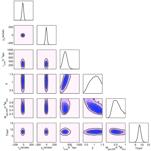
(a) For fitted parameters, posteriors marginalized into two dimensions, and into one dimension along the diagonal.

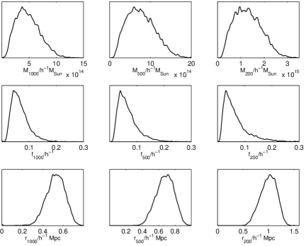
(b) For derived parameters, posteriors marginalized into one dimension.

Figure 5: A773 posterior probability distribution.

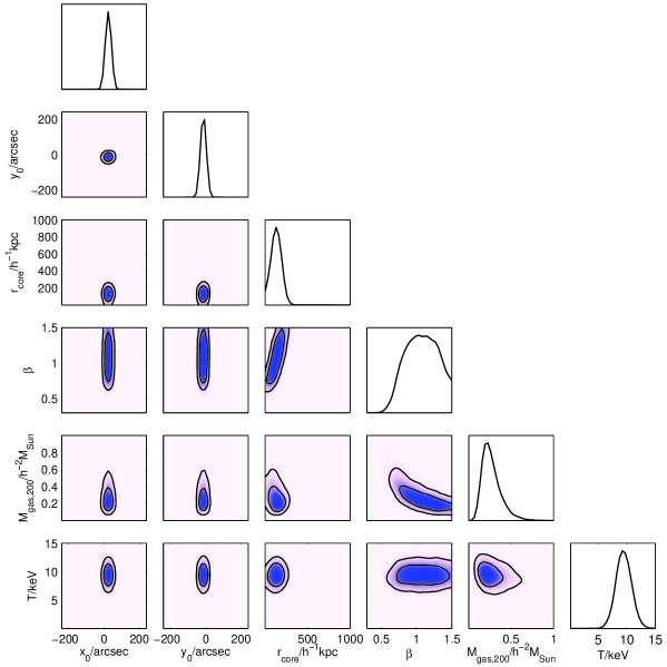
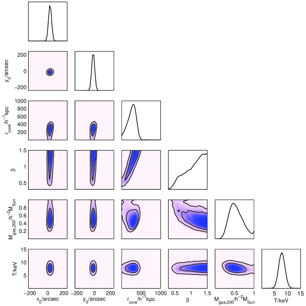
(a) For fitted parameters, posteriors marginalized into two dimensions, and into one dimension along the diagonal.

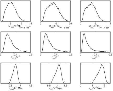
(b) For derived parameters, posteriors marginalized into one dimension.

Figure 6: A1914 posterior probability distribution.

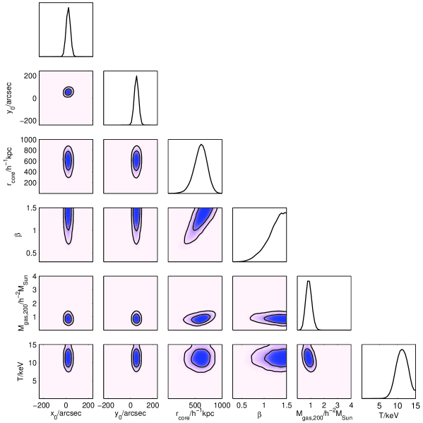
(a) For fitted parameters, posteriors marginalized into two dimensions, and into one dimension along the diagonal.

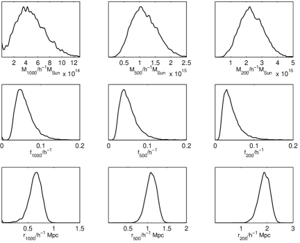
(b) For derived parameters, posteriors marginalized into one dimension.

Figure 7: A2218 posterior probability distribution.

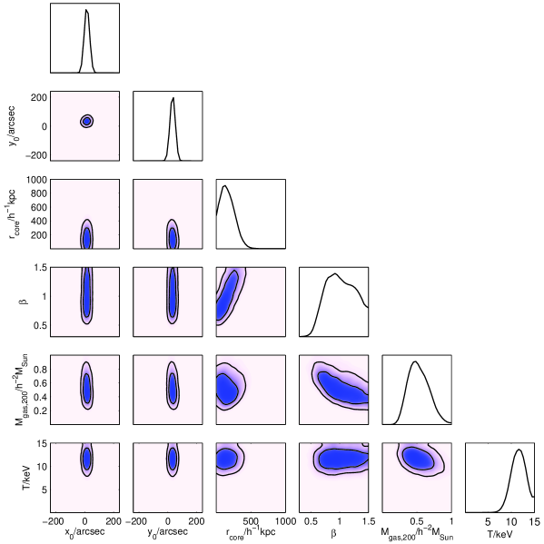
(a) For fitted parameters, posteriors marginalized into two dimensions, and into one dimension along the diagonal.

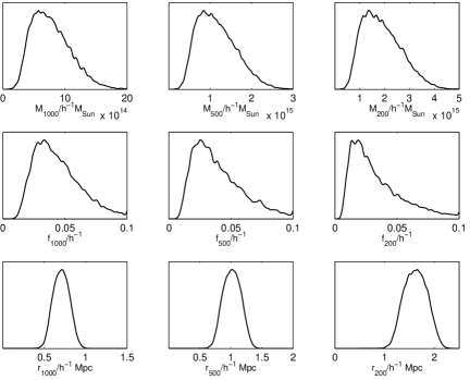
(b) For derived parameters, posteriors marginalized into one dimension.

Figure 8: MACSJ0308+26 posterior probability distribution.

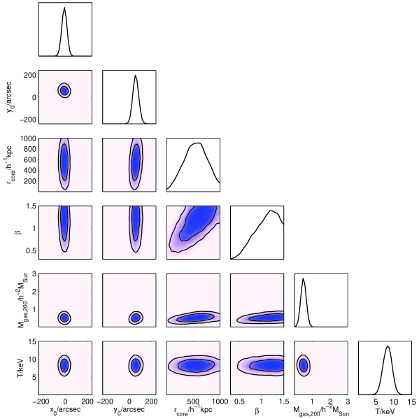
(a) For fitted parameters, posteriors marginalized into two dimensions, and into one dimension along the diagonal.

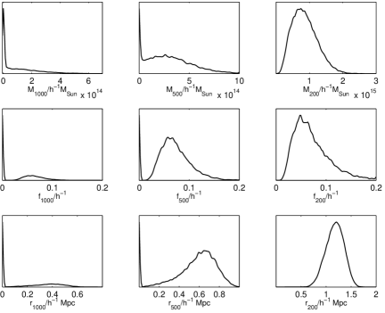
(b) For derived parameters, posteriors marginalized into one dimension.

Figure 9: MACSJ0717+37 posterior probability distribution.

(a) For fitted parameters, posteriors marginalized into two dimensions, and into one dimension along the diagonal.

(b) For derived parameters, posteriors marginalized into one dimension.

Figure 10: MACSJ0744+39 posterior probability distribution.

The full posterior probability distributions for the seven clusters are shown in Figures 5–10. In each figure, the upper panel shows the posterior distributions for the fitted parameters, marginalized into two dimensions, and into one dimension along the diagonal; the lower panel shows the one-dimensional marginalized posterior distributions for parameters derived from those that were fitted. In Table 7 we give mean a posteriori parameter estimates for the clusters, but we caution against their use independently of the posterior probability distributions.

There are two technical points of which to be aware. First, some of the distributions have rough sections. This roughness is just the noise due to the finite numbers of samples. We have used narrow binning of parameter values to avoid misleading effects of averaging especially at distribution edges, with the consequence of high noise per bin. Second, there is a possibility that, for some combination of cluster parameters, nowhere in the cluster does the density reach $a\times\rho_{\mathrm{crit}}$, resulting in no physical solution for $r_{a}$. We set $r_{a}$ to zero in such cases. Out of the seven clusters analysed in this paper, this affected only MACSJ0744+39, resulting in a sharp peak in the posterior probability of $r_{1000}/h^{-1}$Mpc and $r_{500}/h^{-1}$Mpc close to zero radius. Consequently the posterior probability also peaks close to zero for derived parameters $f_{1000}/h^{-1}$, $f_{500}/h^{-1}$, $M_{1000}/h^{-1}M_{\odot}$ and $M_{500}/h^{-1}M_{\odot}$, for this cluster. A different SA configuration or more integration would help for MACSJ0744+39, but at mean overdensity 200 there is no issue.

To set these results in context, we give examples from the literature of other estimates of some of these quantities that we can find for these clusters.

For A611, Schmidt & Allen (2007) using Chandra find a total virial mass of $6.2^{+3.8}_{-1.8}\times 10^{14}M_{\odot}$. From gravitational lensing, Romano et al. (2010) find $r_{200}$ is some 1.5 Mpc and total mass is some 4–7$\times 10^{14}M_{\odot}$.

For A773, Zhang et al. (2008) find from XMM-Newton that $r_{500}$ is 1.3 Mpc, $M_{500}$ is $8.3\pm 2.5\times 10^{14}M_{\odot}$ and $f_{g,500}$ is $0.13\pm 0.07$, while Barrena et al. (2007) estimate a virial mass of $1.2$–$2.7\times 10^{15}M_{\odot}$ from Chandra and optical-spectral velocities.

For A1914, Zhang et al. (2008) find from XMM-Newton that $r_{500}$ is 1.7 Mpc, $M_{500}$ is $16.8\pm 4.9\times 10^{14}M_{\odot}$ and $f_{g,500}$ is $0.07\pm 0.04$. Mroczkowski et al. (2009) fit jointly to Chandra and SZA data and find $r_{200}$ is 1.3 Mpc, $M_{500}$ is $6.6$–$8.1\times 10^{14}M_{\odot}$, and $f_{g,500}$ is $0.14$–$0.16$, the exact values depending on assumptions, with random errors in addition. Zhang et al. (2010) find from XMM-Newton that $M_{1000}$ is $4.36\pm 1.22\times 10^{14}M_{\odot}$ and $M_{500}$ is $7.69\pm 2.24\times 10^{14}M_{\odot}$, while from weak lensing they find that $M_{1000}$ is $3.35^{+0.50}_{-0.47}\times 10^{14}M_{\odot}$ and $M_{500}$ is $4.46^{+0.75}_{-0.69}\times 10^{14}M_{\odot}$.

For A2218, Zhang et al. (2008) find from XMM-Newton that $r_{500}$ is 1.1 Mpc, $M_{500}$ is $4.2\pm 1.3\times 10^{14}M_{\odot}$ and $f_{g,500}$ is $0.15\pm 0.09$.

For MACSJ0744+39, Ettori et al. (2009) find from Chandra that $r_{200}$ is $1566\pm 56$ kpc, and also from Chandra Schmidt & Allen (2007) find a virial mass of $7.4^{+4.4}_{-2.1}\times 10^{14}M_{\odot}$.

Returning to our results, three points that are immediately apparent are that: the gas fractions are low and get lower as $r$ increases; as well as the usual $\beta$–$r_{\mathrm{core}}$ degeneracy (Grego et al., 2001; Grainge et al., 2002; Saunders et al., 2003), there is a tendency to high $\beta$; and the results go out to larger radius than typically obtained from X-ray or SZ cluster analyses. We next consider these points in more detail.

6.1 Masses and gas fractions

Rather than rising towards a canonical large-scale gas fraction of, say, 0.15 as one goes to large $r$ (see e.g. McCarthy et al. 2007, Komatsu et al. 2009, Ettori et al. 2009), our $f_{g}$ values are low and get smaller as $r$ increases. We suspect that our assumption of isothermality may be the cause. If, away from the central region, $T_{\mathrm{e}}(r)$ keeps falling as $r$ increases, then of course our isothermal assumption is invalid. The consequences of this for estimating $M$ and $f_{g}$ are however somewhat worse than we initially expected, for the following reason. In the literature, it is assumed that the value for $M_{r}$ based on hydrostatic equilibrium (equation (5) in this work) implies $M_{r}\propto T_{\mathrm{e}}$. But one has to use equation (5) in terms of radius $r_{a}$ internal to which there is a specific mean overdensity $a$. At a particular $r_{a}$, one can equate $M_{r}$ from equation (5) with the expression for $M_{r}$ from integrating over spherical shells, finding that $r_{a}\propto T^{1/2}$ and in fact $M_{r}\propto T^{3/2}$ (please note our stated convention at the end of section 1). Since $M_{\mathrm{gas},r}\propto T^{-1}$ (given the SZ measurement), $f_{\mathrm{gas},r}$ is proportional to $T^{-5/2}$ rather than the $T^{-2}$ in the literature. It is not possible here to make an approximate quantitative estimate of the effects of the isothermal assumption because of its separate effects on $r_{c}$, on $\beta$, and on total and gas masses as functions of $r$. Nevertheless, if temperatures are less than we have assumed, our total mass estimates are biased high, our gas fraction estimates are biased low, and our $r_{a}$ estimates are somewhat biased high.

6.2 Reaching high radius

Lacey & Cole (1993) give an expression for how the classical virial radius ($r_{178}$ at $z=0$) changes with $z$ in an ${\Omega}-{\Lambda}$ universe: for our lowest and highest cluster redshifts, the virial radii are approximately $r_{205}$ and $r_{215}$. The SA’s sensitivity to structures out to diameters of 10′corresponds to sensitivity to a physical diameter of 1.7 Mpc at our lowest cluster redshift. Given that our $r_{200}$ estimate is biased high, our plots at overdensity 200 thus reach the virial radius in our nearer clusters with some extrapolation of the SZ signal and with no extrapolation in the more-distant ones.

6.3 $\beta$

Typical low-$r$ $\beta$-values are about 0.7 (see e.g. Jones & Forman 1984; Mohr et al. 1999; Ettori et al. 2004) and reach about 0.9 by $r_{1000}$ (see e.g. Vikhlinin et al. 1999; Hallman et al. 2007). Despite the $\beta$–$r_{\mathrm{core}}$ degeneracy, when we marginalize over everything but $\beta$ we find that $\beta$ is much larger. The two likely reasons for this are that our data go to high $r$ and that our estimates of $M_{\mathrm{gas}}$ are biased low at high $r$ because the $T_{\mathrm{e}}$ we use there is too high; at present we cannot assess the relative contributions of these two factors.

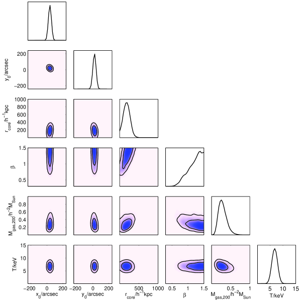
(a) For fitted parameters, posteriors marginalized into two dimensions, and into one dimension along the diagonal.

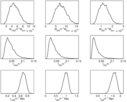
Figure 4: A611 posterior probability distribution.

Table 7: Mean a posteriori parameter estimates with 68 per cent confidence limits. Note that $e^{x}$ means $10^{x}$ in this table.

	A611	A773	A1914	A2218
$r_{\mathrm{core}}/$kpc	$2.6e+02^{5.4e+01}_{-6.0e+01}$	$3.8e+02^{1.5e+02}_{-1.5e+02}$	$1.9e+02^{3.6e+01}_{-3.9e+01}$	$3.7e+02^{8.2e+01}_{-5.8e+01}$
$\beta$	$1.2e+00^{2.9e-01}_{-8.2e-02}$	$1.0e+00^{4.9e-01}_{-1.4e-01}$	$1.1e+00^{4.3e-01}_{-1.2e-01}$	$1.1e+00^{4.1e-01}_{-1.3e-01}$
$M_{\mathrm{gas},200}/M_{\odot}$	$6.0e+13^{7.1e+12}_{-1.2e+13}$	$1.2e+14^{1.6e+13}_{-2.7e+13}$	$5.5e+13^{5.3e+12}_{-1.3e+13}$	$1.1e+14^{1.3e+13}_{-2.2e+13}$
$M_{1000}/M_{\odot}$	$7.2e+14^{1.0e+14}_{-1.3e+14}$	$6.9e+14^{1.3e+14}_{-1.8e+14}$	$1.2e+15^{1.7e+14}_{-2.3e+14}$	$7.6e+14^{1.4e+14}_{-1.8e+14}$
$M_{500}/M_{\odot}$	$1.1e+15^{1.6e+14}_{-2.0e+14}$	$1.1e+15^{2.1e+14}_{-2.8e+14}$	$1.7e+15^{2.5e+14}_{-3.5e+14}$	$1.2e+15^{2.4e+14}_{-2.8e+14}$
$M_{200}/M_{\odot}$	$1.8e+15^{2.7e+14}_{-3.2e+14}$	$1.9e+15^{3.7e+14}_{-4.8e+14}$	$2.7e+15^{4.0e+14}_{-5.6e+14}$	$2.0e+15^{4.2e+14}_{-4.8e+14}$
$r_{1000}/$Mpc	$6.8e-01^{4.1e-02}_{-3.7e-02}$	$5.3e-01^{4.7e-02}_{-3.9e-02}$	$8.3e-01^{5.1e-02}_{-4.9e-02}$	$7.1e-01^{5.7e-02}_{-4.7e-02}$
$r_{500}/$Mpc	$9.8e-01^{5.9e-02}_{-5.2e-02}$	$6.8e-01^{5.7e-02}_{-4.9e-02}$	$1.2e+00^{7.4e-02}_{-7.1e-02}$	$1.0e+00^{8.9e-02}_{-6.7e-02}$
$r_{200}/$Mpc	$1.6e+00^{9.6e-02}_{-8.1e-02}$	$1.0e+00^{8.6e-02}_{-7.1e-02}$	$1.9e+00^{1.2e-01}_{-1.1e-01}$	$1.7e+00^{1.5e-01}_{-1.1e-01}$
$f_{1000}$	$6.4e-02^{7.5e-03}_{-1.9e-02}$	$9.5e-02^{1.2e-02}_{-2.6e-02}$	$3.8e-02^{4.1e-03}_{-1.3e-02}$	$9.5e-02^{9.5e-03}_{-3.0e-02}$
$f_{500}$	$5.3e-02^{5.7e-03}_{-1.8e-02}$	$9.5e-02^{1.2e-02}_{-3.1e-02}$	$3.3e-02^{2.8e-03}_{-1.3e-02}$	$8.9e-02^{5.2e-03}_{-3.6e-02}$
$f_{200}$	$4.1e-02^{2.8e-03}_{-1.7e-02}$	$9.5e-02^{8.5e-03}_{-4.0e-02}$	$2.7e-02^{1.2e-03}_{-1.3e-02}$	$8.3e-02^{4.3e-03}_{-4.4e-02}$

	MACSJ0308+26	MACSJ0717+37	MACSJ0744+39
$r_{\mathrm{core}}/$kpc	$8.6e+02^{8.3e+01}_{-6.7e+01}$	$2.4e+02^{5.7e+01}_{-8.3e+01}$	$7.8e+02^{1.5e+02}_{-1.5e+02}$
$\beta$	$1.2e+00^{2.6e-01}_{-6.2e-02}$	$1.0e+00^{4.8e-01}_{-1.4e-01}$	$1.1e+00^{4.0e-01}_{-1.1e-01}$
$M_{\mathrm{gas},200}/M_{\odot}$	$1.8e+14^{1.6e+13}_{-2.0e+13}$	$1.1e+14^{1.3e+13}_{-1.7e+13}$	$1.0e+14^{1.1e+13}_{-1.2e+13}$
$M_{1000}/M_{\odot}$	$7.0e+14^{1.4e+14}_{-7.0e+14}$	$1.1e+15^{1.7e+14}_{-2.6e+14}$	$1.3e+14^{1.8e+14}_{-1.3e+14}$
$M_{500}/M_{\odot}$	$1.7e+15^{2.4e+14}_{-3.2e+14}$	$1.7e+15^{2.7e+14}_{-4.1e+14}$	$4.4e+14^{1.2e+14}_{-4.4e+14}$
$M_{200}/M_{\odot}$	$3.4e+15^{4.9e+14}_{-5.6e+14}$	$2.7e+15^{4.5e+14}_{-6.8e+14}$	$1.2e+15^{2.1e+14}_{-3.0e+14}$
$r_{1000}/$Mpc	$6.4e-01^{6.4e-02}_{-4.4e-02}$	$7.1e-01^{4.8e-02}_{-4.9e-02}$	$2.1e-01^{1.5e-01}_{-2.1e-01}$
$r_{500}/$Mpc	$1.1e+00^{6.8e-02}_{-6.0e-02}$	$1.0e+00^{7.2e-02}_{-7.3e-02}$	$5.7e-01^{1.1e-01}_{-5.7e-01}$
$r_{200}/$Mpc	$1.9e+00^{1.1e-01}_{-9.0e-02}$	$1.6e+00^{1.2e-01}_{-1.2e-01}$	$1.2e+00^{9.2e-02}_{-8.1e-02}$
$f_{1000}$	$8.4e-02^{9.2e-03}_{-1.9e-02}$	$6.5e-02^{8.4e-03}_{-1.8e-02}$	$5.5e-02^{3.0e-02}_{-5.5e-02}$
$f_{500}$	$7.5e-02^{7.8e-03}_{-1.9e-02}$	$5.9e-02^{7.9e-03}_{-2.0e-02}$	$1.0e-01^{1.6e-02}_{-1.0e-01}$
$f_{200}$	$6.1e-02^{5.8e-03}_{-1.9e-02}$	$5.2e-02^{5.8e-03}_{-2.2e-02}$	$1.0e-01^{1.3e-02}_{-3.2e-02}$

7 Conclusions

1. Untapered, naturally-weighted AMI Small Array maps at 13.9–18.2 GHz, with no source subtraction, show clear SZ effects in five of the seven clusters.

2. Using source-subtraction observations that are largely from the Ryle Telescope (and thus at $15$ GHz but typically two years before the SA observations), and assuming a spherical $\beta$-model, hydrostatic equilibrium, and isothermality with an X-ray measured temperature, our Bayesian analysis reveals SZ signals in all seven clusters. In six of these, the Bayesian evidence for an SZ detection, in addition to sources plus CMB primary anisotropies plus thermal noise, is huge; in the one of them with much the worst thermal noise, there is a 1 in 3000 chance that the SZ is spurious. We emphasize that, to allow for variability, we set the prior on each source’s flux density as its high-resolution value with a Gaussian 1-$\sigma$ width of (except in one case) $\pm 30$ per cent.

3. The Bayesian evidence proves very useful in understanding source environments. For example, a high-resolution map showed a feature that, by eye, was classed as a tentative radio-source detection. Running the Bayesian analysis twice, with and without that tentative source, showed that the evidence for it is in fact so low that it should not be included.

4. We note that our sensitivity to structures out to 10′, corresponding to a 1.7-Mpc diameter for our lowest-redshift cluster, means that our parameter estimates out to the classical virial radii of the nearer clusters involve some extrapolation, but no extrapolation is needed for the more-distant ones.

5. Our probability distributions of masses and radii internal to which the average overdensities are 1000, 500 and 200 are usefully constrained and change sensibly over this range. However, our gas fractions are evidently low compared with values in the literature; further, they decrease with increasing radius, which is also unexpected. The problem seems consistent with the notion that temperature $T_{\mathrm{e}}$ decreases as radius $r$ increases whereas we are assuming issothermality (using temperatures measured from low-radii data); the problem is made somewhat worse because, as we have shown, gas fraction goes as $T_{\mathrm{e}}^{-2.5}$ assuming isothermality and hydrostatic equilibrium rather than as $T_{\mathrm{e}}^{-2}$ as seems to have been assumed in the literature. If $T_{\mathrm{e}}$ does indeed fall as $r$ increases, our gas masses are biased low and our total masses (and to a lesser extent our measurements of $r_{a}$) are biased high. Temperature profiles must be measured or some other means found to deal with this problem if we are to infer masses out towards the virial radius. Indeed, along with other density-profile models, this will be investigated in future work.

References

- AMI Consortium: Franzen et al. (2009) AMI Consortium: Franzen T. M. O., et al., 2009, MNRAS, 400, 995
- AMI Consortium: Hurley-Walker et al. (2009a) AMI Consortium: Hurley-Walker N., et al., 2009a, MNRAS, 396, 365
- AMI Consortium: Hurley-Walker et al. (2009b) AMI Consortium: Hurley-Walker N., et al., 2009b, MNRAS, 398, 249
- AMI Consortium: Scaife et al. (2008) AMI Consortium: Scaife A. M. M., et al., 2008, MNRAS, 385, 809
- AMI Consortium: Scaife et al. (2009a) AMI Consortium: Scaife A. M. M., et al., 2009a, MNRAS, 400, 1394
- AMI Consortium: Scaife et al. (2009b) AMI Consortium: Scaife A. M. M., et al., 2009b, MNRAS, 394, L46
- AMI Consortium: Zwart et al. (2008) AMI Consortium: Zwart J. T. L., et al., 2008, MNRAS, 391, 1545
- Andersson et al. (2010) Andersson K., Benson B. A., Ade P. A. R., et al., 2010, preprint: astro-ph.CO/1006.3068
- Böhringer et al. (2000) Böhringer H., et al., 2000, ApJS, 129, 435
- Balestra et al. (2007) Balestra I., Tozzi P., Ettori S., Rosati P., Borgani S., Mainieri V., Norman C., Viola M., 2007, A&A, 462, 429
- Barrena et al. (2007) Barrena R., Boschin W., Girardi M., Spolaor M., 2007, A&A, 467, 37
- Bautz et al. (2009) Bautz M. W., Miller E. D., Sanders J. S., Arnaud K. A., Mushotzky R. F., Porter F. S., Hayashida K., Henry J. P., Hughes J. P., Kawaharada M., Makashima K., Sato M., Tamura T., 2009, PASJ, 61, 1117
- Birkinshaw (1999) Birkinshaw M., 1999, Phys. Rep., 310, 97
- Bolton et al. (2006) Bolton R. C., Chandler C. J., Cotter G., Pearson T. J., Pooley G. G., Readhead A. C. S., Riley J. M., Waldram E. M., 2006, MNRAS, 370, 1556
- Bonamente et al. (2008) Bonamente M., Joy M., LaRoque S. J., Carlstrom J. E., Nagai D., Marrone D. P., 2008, ApJ, 675, 106
- Carlstrom et al. (2009) Carlstrom J. E., Ade P. A. R., Aird K. A., et al., 2009, preprint: astro-ph.IM/0907.4445
- Carlstrom et al. (2002) Carlstrom J. E., Holder G. P., Reese E. D., 2002, ARA&A, 40, 643
- Condon et al. (1998) Condon J. J., Cotton W. D., Greisen E. W., Yin Q. F., Perley R. A., Taylor G. B., Broderick J. J., 1998, AJ, 115, 1693
- Cotter et al. (2002) Cotter G., Buttery H. J., Das R., Jones M. E., Grainge K., Pooley G. G., Saunders R., 2002, MNRAS, 334, 323
- Cotter et al. (2002) Cotter G., et al., 2002, MNRAS, 331, 1
- Culverhouse et al. (2010) Culverhouse T. L., Bonamente M., Bulbul E., et al., 2010, preprint: astro-ph.CO/1007.2853
- De Grandi & Molendi (2002) De Grandi S., Molendi S., 2002, ApJ, 567, 163
- Dobbs et al. (2006) Dobbs M., Halverson N. W., Ade P. A. R., et al., 2006, New Astronomy Review, 50, 960
- Donnarumma et al. (2010) Donnarumma A., Ettori S., Meneghetti M., Gavazzi R., Fort B., Moscardini L., Romano A., Fu L., Giordano F., Radovich M., Maoli R., Scaramella R., Richard J., 2010, preprint: astro-ph.CO/1002.1625
- Ebeling et al. (2004) Ebeling H., Barrett E., Donovan D., 2004, ApJ, 609, L49
- Ebeling et al. (2007) Ebeling H., Barrett E., Donovan D., Ma C.-J., Edge A. C., van Speybroeck L., 2007, ApJ, 661, L33
- Ebeling et al. (2001) Ebeling H., Edge A. C., Henry J. P., 2001, ApJ, 553, 668
- Ebeling et al. (2010) Ebeling H., Edge A. C., Mantz A., Barrett E., Henry J. P., Ma C. J., van Speybroeck L., 2010, MNRAS, p. 962
- Edge et al. (2003) Edge A. C., Ebeling H., Bremer M., Röttgering H., van Haarlem M. P., Rengelink R., Courtney N. J. D., 2003, MNRAS, 339, 913
- Ettori et al. (2009) Ettori S., Morandi A., Tozzi P., Balestra I., Borgani S., Rosati P., Lovisari L., Terenziani F., 2009, A&A, 501, 61
- Ettori et al. (2004) Ettori S., Tozzi P., Borgani S., Rosati P., 2004, A&A, 417, 13
- Feroz & Hobson (2008) Feroz F., Hobson M. P., 2008, MNRAS, 384, 449
- Feroz et al. (2009) Feroz F., Hobson M. P., Zwart J. T. L., Saunders R. D. E., Grainge K. J. B., 2009, MNRAS, 398, 2049
- George et al. (2009) George M. R., Fabian A. C., Sanders J. S., Young A. J., Russell H. R., 2009, MNRAS, 395, 657
- Govoni et al. (2004) Govoni F., Markevitch M., Vikhlinin A., van Speybroeck L., Feretti L., Giovannini G., 2004, ApJ, 605, 695
- Grainge et al. (2002) Grainge K., Grainger W. F., Jones M. E., Kneissl R., Pooley G. G., Saunders R., 2002, MNRAS, 329, 890
- Grainge et al. (1996) Grainge K., Jones M., Pooley G., Saunders R., Baker J., Haynes T., Edge A., 1996, MNRAS, 278, L17
- Grainge et al. (1993) Grainge K., Jones M., Pooley G., Saunders R., Edge A., 1993, MNRAS, 265, L57
- Grainge et al. (2002) Grainge K., Jones M. E., Pooley G., Saunders R., Edge A., Grainger W. F., Kneissl R., 2002, MNRAS, 333, 318
- Grainger et al. (2002) Grainger W. F., Das R., Grainge K., Jones M. E., Kneissl R., Pooley G. G., Saunders R. D. E., 2002, MNRAS, 337, 1207
- Grego et al. (2001) Grego L., Carlstrom J. E., Reese E. D., Holder G. P., Holzapfel W. L., Joy M. K., Mohr J. J., Patel S., 2001, ApJ, 552, 2
- Hallman et al. (2007) Hallman E. J., Burns J. O., Motl P. M., Norman M. L., 2007, ApJ, 665, 911
- Ho et al. (2009) Ho P. T. P., Altamirano P., Chang C., et al., 2009, ApJ, 694, 1610
- Hobson & Maisinger (2002) Hobson M. P., Maisinger K., 2002, MNRAS, 334, 569
- Hoshino et al. (2010) Hoshino A., Patrick Henry J., Sato K., Akamatsu H., Yokota W., Sasaki S., Ishisaki Y., Ohashi T., Bautz M., Fukazawa Y., Kawano N., Furuzawa A., Hayashida K., Tawa N., Hughes J. P., Kokubun M., Tamura T., 2010, PASJ, 62, 371
- Irwin et al. (1999) Irwin J. A., Bregman J. N., Evrard A. E., 1999, ApJ, 519, 518
- Jones & Forman (1984) Jones C., Forman W., 1984, ApJ, 276, 38
- Jones et al. (2005) Jones M. E., et al., 2005, MNRAS, 357, 518
- Komatsu et al. (2009) Komatsu E., Dunkley J., Nolta M. R., et al., 2009, ApJS, 180, 330
- Lacey & Cole (1993) Lacey C., Cole S., 1993, MNRAS, 262, 627
- LaRoque et al. (2006) LaRoque S. J., Bonamente M., Carlstrom J. E., Joy M. K., Nagai D., Reese E. D., Dawson K. S., 2006, ApJ, 652, 917
- Leccardi & Molendi (2008) Leccardi A., Molendi S., 2008, A&A, 486, 359
- Markevitch et al. (1998) Markevitch M., Forman W. R., Sarazin C. L., Vikhlinin A., 1998, ApJ, 503, 77
- Marshall et al. (2003) Marshall P. J., Hobson M. P., Slosar A., 2003, MNRAS, 346, 489
- McCarthy et al. (2007) McCarthy I. G., Bower R. G., Balogh M. L., 2007, MNRAS, 377, 1457
- Menanteau et al. (2010) Menanteau F., Gonzalez J., Juin J., et al., 2010, preprint: astro-ph.CO/1006.5126
- Mohr et al. (1999) Mohr J. J., Mathiesen B., Evrard A. E., 1999, ApJ, 517, 627
- Mroczkowski et al. (2009) Mroczkowski T., et al., 2009, ApJ, 694, 1034
- Peebles (1993) Peebles J., 1993, Principles of Physical Cosmology. Princeton: Princeton University Press
- Pratt et al. (2005) Pratt G. W., Böhringer H., Finoguenov A., 2005, A&A, 433, 777
- Romano et al. (2010) Romano A., Fu L., Giordano F., et al., 2010, A&A, 514, A88
- Sadler et al. (2006) Sadler E. M., et al., 2006, MNRAS, 371, 898
- Saunders et al. (2003) Saunders R., Kneissl R., Grainge K., et al., 2003, MNRAS, 341, 937
- Schmidt & Allen (2007) Schmidt R. W., Allen S. W., 2007, MNRAS, 379, 209
- Struble & Rood (1999) Struble M. F., Rood H. J., 1999, ApJS, 125, 35
- Sunyaev & Zeldovich (1970) Sunyaev R. A., Zeldovich Y. B., 1970, Comments on Astrophysics and Space Physics, 2, 66
- Sunyaev & Zeldovich (1972) Sunyaev R. A., Zeldovich Y. B., 1972, Comments on Astrophysics and Space Physics, 4, 173
- Swetz et al. (2010) Swetz D. S., Ade P. A. R., Amiri M., et al., 2010, preprint: astro-ph.IM/1007.0290
- Vikhlinin et al. (1999) Vikhlinin A., Forman W., Jones C., 1999, ApJ, 525, 47
- Vikhlinin et al. (2005) Vikhlinin A., Markevitch M., Murray S. S., Jones C., Forman W., Van Speybroeck L., 2005, ApJ, 628, 655
- Waldram et al. (2007) Waldram E. M., Bolton R. C., Pooley G. G., Riley J. M., 2007, MNRAS, 379, 1442
- Waldram et al. (2003) Waldram E. M., Pooley G. G., Grainge K. J. B., Jones M. E., Saunders R. D. E., Scott P. F., Taylor A. C., 2003, MNRAS, 342, 915
- Wu et al. (2009) Wu J., Ho P. T. P., Huang C., et al., 2009, ApJ, 694, 1619
- Zhang et al. (2008) Zhang Y., Finoguenov A., Böhringer H., Kneib J., Smith G. P., Kneissl R., Okabe N., Dahle H., 2008, A&A, 482, 451
- Zhang et al. (2010) Zhang Y., Okabe N., Finoguenov A., et al., 2010, ApJ, 711, 1033