Time-dependent Stochastic Modeling of Solar Active Region Energy

Abstract

A time-dependent model for the energy of a flaring solar active region is presented based on an existing stochastic jump-transition model [Wheatland and Glukhov (1998), Wheatland (2008), Wheatland (2009)]. The magnetic free energy of an active region is assumed to vary in time due to a prescribed (deterministic) rate of energy input and prescribed (random) jumps downwards in energy due to flares. The existing model reproduces observed flare statistics, in particular flare frequency-size and waiting-time distributions, but modeling presented to date has considered only the time-independent choices of constant energy input and constant flare transition rates with a power-law distribution in energy. These choices may be appropriate for a solar active region producing a constant mean rate of flares. However, many solar active regions exhibit time variation in their flare productivity, as exemplified by NOAA active region AR 11029, observed during October-November 2009 [Wheatland (2010)]. Time variation is incorporated into the jump-transition model for two cases: 1. a step change in the rates of flare transitions; and 2. a step change in the rate of energy supply to the system. Analytic arguments are presented describing the qualitative behavior of the system in the two cases. In each case the system adjusts by shifting to a new stationary state over a relaxation time which is estimated analytically. The model exhibits flare-like event statistics. In each case the frequency-energy distribution is a power law for flare energies less than a time-dependent rollover set by the largest energy the system is likely to attain at a given time. The rollover is not observed if the mean free energy of the system is sufficiently large. For Case 1, the model exhibits a double exponential waiting-time distribution, corresponding to flaring at a constant mean rate during two intervals (before and after the step change), if the average energy of the system is large. For Case 2 the waiting-time distribution is a simple exponential, again provided the average energy of the system is large. Monte Carlo simulations of Case 1 are presented which confirm the estimate for the relaxation time, and confirm the expected forms of the frequency-energy and waiting-time distributions. The simulation results provide a qualitative model for observed flare statistics in active region AR 11029.

1 Introduction

sec:Introduction

Solar flares are magnetic explosions in the Sun’s outer atmosphere, the corona, which occur intermittently. Local space weather effects due to large flares, including damage to electronics on expensive communications satellites, motivate attempts to predict flare occurrence [Odenwald, Green and Taylor (2006), Committee On The Societal & Economic Impacts Of Severe Space Weather Events (2008)]. However, existing prediction methods are probabilistic, and not very reliable [Wheatland (2005), Barnes and Leka (2008)].

The flare mechanism is believed to be magnetic reconnection, which occurs at certain topological sites in the coronal magnetic field configuration of active regions around sunspots [Priest and Forbes (2002)]. However, the reconnection process is incompletely understood, and detailed observations of individual flares reveal a diversity of effects which are often secondary phenomena, providing only indirect information on the underlying flare mechanism [Benz (2008)]. The statistics of solar flare occurrence have been examined in an attempt to provide insight into the flare phenomenon, and also to improve flare prediction.

1.1 Observed flare statistics

subsec:ObsStats

Two statistical distributions of interest are the flare frequency-size distribution, and the waiting-time distribution. The frequency-size distribution ${\cal N}(S)$ is the number of events per unit time and per unit size $S$, where ‘size’ refers to a measure of the magnitude of an event, for example the peak flux in X-ray wavelengths, or an estimate of the energy. The frequency-size distribution is observed to be a featureless power-law over many orders of magnitude [Akabane (1956), Aschwanden (2005)]:

$$\ilabel{eq:freq_{s}ize}{\cal N}(S)=\lambda_{1}(\gamma-1)S_{1}^{\gamma-1}S^{-\gamma},$$ (1)

where $\gamma\approx 1.5$–2 is the power-law index (the exact value depends on the choice of the measure for size) and $\lambda_{1}$ is the total mean rate of flaring for events larger than $S_{1}$. Few exceptions to this simple power-law distribution have been reported [see however 2010ApJ…710.1324W], although an upper rollover or cut-off is required on energetics grounds [Hudson (1991)]. The waiting-time distribution is the distribution $P(\Delta t)$ of times $\Delta t$ between flare events. For individual active regions the waiting-time distribution is often observed to be consistent with a simple exponential:

$$\ilabel{eq:wtd_{p}oiss}P(\Delta t)=\lambda_{1}{\rm e}^{-\lambda_{1}\Delta t}.$$ (2)

where $\lambda_{1}$ is the mean rate of events of events defined by Equation (eq:freq_size). This model corresponds to flares occurring as independent random events at a constant mean rate, i.e. as a Poisson process in time [Moon et al. (2001), Wheatland (2001)]. However, the mean rate of flaring in active regions is often observed to vary, in which case a piecewise-constant Poisson model may be appropriate. The model waiting-time distribution is then a sum of exponentials corresponding to distinct intervals with different rates [Wheatland and Litvinenko (2002)]:

$$\ilabel{eq:wtd_{p}const-poiss}P(\Delta t)=\sum_{i}\frac{n_{1i}}{N_{1}}\lambda_{1i}{\rm e}^{-\lambda_{1i}\Delta t},$$ (3)

where $n_{1i}=\lambda_{1i}t_{i}$ is the number of events with size larger than $S_{1}$ corresponding to a rate $\lambda_{1i}$ and an interval $t_{i}$, and where $N_{1}=\sum_{i}n_{1i}$ is the total number of events. A power-law tail is observed in the combined waiting-time distribution for events from multiple active regions over longer periods of time on the Sun [Boffetta et al. (1999)], which also may be accounted for by the time-dependent Poisson model [Wheatland (2000), Wheatland and Litvinenko (2002)], although some authors have argued for a non-Poisson interpretation [Lepreti, Carbone, and Veltri (2001)]. Recently 2010ApJ…717..683A demonstrated that a variety of observations for the longer-term waiting-time distribution are consistent with Poisson occurrence in time according to a simple functional form for the distribution of rates in time, which is a variant of the rate distribution presented in 2000ApJ…536L.109W.

1.2 Flare statistics in two active regions

subsec:TwoARs

To illustrate these ideas we consider two active regions: US National Oceanic and Atmospheric Administration (NOAA) active region AR 10486, from October-November 2003, and NOAA AR 11029, from October-November 2009. The data used are the soft X-ray event lists compiled by the US Space Weather Prediction Center (SWPC). The events are selected from whole-Sun $1$–$8\,\mbox{\AA}$ flux measurements by the Geostationary Observational Environmental satellites (GOES). The peak flux of GOES events is routinely used to classify flares, and is the measure of size used here. The SWPC/GOES data are often used in studies of flare statistics, although they are less than ideal for this purpose because the lists are incomplete, and the peak fluxes in the lists are not background-subtracted [for a discussion see e.g. 2001SoPh..203…87W]. However, the events for active region AR 11029 shown here are individually background subtracted, based on work in an earlier study [Wheatland (2010)].

Figure fig:dists_ar10486 illustrates the frequency-energy, and waiting-time distributions, for soft X-ray flares observed in active region AR 10486. This large and highly complex sunspot region appeared in the late stages of the maximum of the last solar cycle and produced a remarkable sequence of extremely large solar flares [Dun et al. (2007), Chumak, Zhang, and Guo (2008)]. Figure fig:dists_ar10486 shows the events in this region larger than peak flux $S_{1}=3\times 10^{-6}\,{\rm W}\,{\rm m}^{-2}$ (this choice should ensure the list of events is relatively complete, for events larger than $S_{1}$). The region produced $N_{1}=43$ events with peak flux larger than $S_{1}$, including the biggest flare of the modern era (with listed peak flux $2.8\times 10^{-3}\,{\rm W}\,{\rm m}^{-2}$), on 4 November 2003. The upper panel shows the peak fluxes versus the recorded peak times for the events as a sequence of vertical lines, with a logarithmic scaling for flux, the 4 November flare being the tallest line. The middle panel plots the the number of events above size $S$ versus size, which corresponds to the cumulative peak-flux distribution $C(S)$, defined in terms of the frequency-peak flux distribution by

$$\ilabel{eq:cum_{s}ize}C(S)=\frac{T}{N_{1}}\int_{S}^{\infty}{\cal N}(S^{\prime})\,dS^{\prime},$$ (4)

where $T$ is the duration of the observing interval, and $S>S_{1}$. The vertical line in this panel indicates $S_{1}$. The events are approximately power-law distributed in peak flux (a straight line in this representation), consistent with Equation (eq:freq_size). The lower panel plots the waiting-time distribution for the same events, again as a cumulative distribution i.e. the number of waiting times larger than a given time versus waiting time. This corresponds to the integral of $P(\Delta t)$ with respect to $\Delta t$. The distribution is presented with a log-linear scaling, and reveals that the events are approximately exponentially distributed (a straight line, in this representation), consistent with Equation (eq:wtd_poiss).

Figure fig:dists_ar10486 shows that AR 10486, although remarkable in terms of the size of particular events, was unremarkable statistically. It produced flares according to a power-law frequency-peak flux distribution at a constant mean rate during its transit of the disk. This suggests that the physical conditions underlying flaring are approximately time-independent.

Figure 1.: Flares in the GOES events lists for NOAA active region AR 10486 above peak soft X-ray flux $3\times 10^{-6}{\rm W}{\rm m}^{-2}$ (43 events). Upper panel: Schematic showing the peak flux of each event at the event time. Middle panel: The frequency-peak flux distribution, as a cumulative plot in a log-log representation. Lower panel: The waiting-time distribution as a cumulative plot in a log-linear representation.fig:dists˙ar10486

Figure fig:dists_ar11029 shows GOES event data for active region AR 11029, which exhibits time variation in its mean rate of flaring. This spatially small but highly flare-productive active region emerged on the disk in October 2009, during an extended interval of low solar activity. The statistics of events in this region were investigated in 2010ApJ…710.1324W. The presentation of Figure fig:dists_ar11029 is the same as Figure fig:dists_ar10486, but in this case the data are individually background-subtracted, which is particularly important because the events are small. There are $N_{1}=56$ events above a backgrounded-subtracted peak flux of $S_{1}=10^{-7}\,{\rm W}\,{\rm m}^{-2}$, as shown in the upper panel. This panel suggests that the flaring rate is high for two days (26 October and 27 October), and relatively low at other times, an interpretation supported by a Bayesian rate analysis [Scargle (1998), Wheatland (2010)]. The changes in the rate are quite dramatic: a relatively sudden increase by a factor of about ten, and a sudden decrease by about the same factor. The lower panel plots the cumulative waiting-time distribution, which shows a double exponential form, consistent with Poisson occurrence at two different mean rates (a low and a high rate), as represented by Equation (eq:wtd_pconst-poiss) with two intervals/rates. The middle panel in Figure fig:dists_ar11029 plots the cumulative peak-flux distribution for the flares in AR 11029, and is suggestive of a rollover around $10^{-6}\,{\rm W}\,{\rm m}^{-2}$. 2010ApJ…710.1324W applied Bayesian model comparison to show that a power-law plus upper rollover model is much more probable for this data set than a simple power-law model, and argued that the departure from a power law may reflect the finite storage of magnetic energy in this (small) region.

Time variation in mean flaring rate is commonly observed in active regions [Wheatland (2001)], and is often associated, as in the case of active region AR 11029, with a change in the photospheric magnetic complexity of a region [Wheatland (2010)]. On October 26 the region increased in photospheric magnetic complexity (becoming a $\beta$–$\gamma$ region, in the Mt Wilson classification), coincident with the increase in flaring rate. Photospheric magnetic field changes are likely to be reflected in changes in the magnetic field configuration in the corona, which may facilitate or inhibit reconnection, and hence change the flaring rate. It is plausible that the more interesting statistics observed for AR 11029, by comparison with AR 10486 (Figure fig:dists_ar10486) are related to the smaller physical smaller size of the region, which may make the coronal magnetic field configuration more sensitive to change.

Figure 2.: Flares in the GOES events lists for NOAA active region AR 11029 with a background-subtracted peak flux above $10^{-7}\,{\rm W}{\rm m}^{-2}$, a total of 56 events (Wheatland 2010). The presentation of the data is the same as in Figure 1.fig:dists˙ar11029

1.3 Models for flare statistics

subsec:ModStats

Models for solar flare statistics attempt to account for the observed distributions. Most of the models are motivated either by accounting for energy balance in an active region [Rosner and Vaiana (1978), Litvinenko (1994), Craig (2001)] or by explaining the power law in the frequency-size distribution using self-organized criticality/cellular automata (‘avalanche’ models) [Lu and Hamilton (1991), Charbonneau et al. (2001), Hughes et al. (2003)], although the two pictures are not mutually exclusive. The avalanche model produces a power-law frequency-size distribution below an upper rollover set by the size of the cellular automata [Lu et al. (1993)], and has an exponential (Poisson) waiting-time distribution, if the system is subject to a constant mean rate of driving [Biesecker (1994), (40)], but may produce other waiting-time distributions with time-dependent driving [Norman et al. (2001)]. Energy balance models are designed to explain the power-law frequency-energy distribution, and generally assume Poisson flare occurrence, but simple models in which active region energy is completely removed by a flare imply a relationship between waiting times and energy, which is not observed [Lu (1995)]. A generalized energy-balance formalism (a ‘jump-transition model’) which avoids this problem was introduced by 1998ApJ…494..858W, and further developed in 2008ApJ…679.1621W and 2009SoPh..255..211W. The jump-transition model is applied in this paper.

The general jump-transition model [Wheatland and Glukhov (1998), Wheatland (2008), Wheatland (2009)] describes the magnetic free energy $E=E(t)$ of an active region at time $t$ in terms of secular energy input at a rate $\beta(E,t)$, and stochastic transitions downwards in energy (flares) at a rate $\alpha(E,E^{\prime},t)$ per unit time and per unit energy for transitions from $E$ to $E^{\prime}$. The model may be presented either in terms of an integro-partial differential equation describing the probability distribution $P(E,t)$ for the energy [Wheatland and Glukhov (1998), Wheatland (2008)], called a ‘master equation’ [van Kampen (1992), Gardiner (2004)], or in terms of a stochastic differential equation describing the time evolution of $E=E(t)$ [Wheatland (2009)].

Modeling using the jump-transition formalism to date has considered only time-independent cases, namely a time- and energy-independent rate of energy input:

$$\ilabel{eq:beta_{w}g98}\beta(E)=\beta_{0},$$ (5)

where $\beta_{0}$ is a constant, and time-independent power-law distributed flare transitions:

$$\ilabel{eq:pl_{a}lpha_{w}g98}\alpha(E,E^{\prime})=\alpha_{0}(E-E^{\prime})^{-\gamma}\theta(E-E^{\prime}-E_{c}),$$ (6)

where $\alpha_{0}$ is a constant, $E_{c}$ is a low-energy cutoff, $\theta(x)$ denotes the step function, and $\gamma=1.5$ is the observed power-law index in the flare frequency-energy distribution [Aschwanden (2005)]. The model flare frequency-energy distribution is given by

eq:ffe˙pl˙alpha$${\cal N}(E) = \int_{E}^{\infty}P(E^{\prime})\alpha(E^{\prime},E^{\prime}-E){\mathrm{d}}E^{\prime}$$ (7)

$$= \alpha_{0}E^{-\gamma}\int_{E}^{\infty}P(E^{\prime}){\mathrm{d}}E^{\prime}\quad\mbox{for}\quad E\geq E_{c},$$

and is zero for $E<E_{c}$. Equation (eq:ffe_pl_alpha) describes a power law with index $\gamma$ above $E_{c}$ and below an upper rollover set by the largest energy the system is likely to attain, which has an approximate lower bound given by the estimate for the average or mean energy of the system [Wheatland (2008)]:

$$\ilabel{eq:Ea}{\cal E}=\left(\frac{2-\gamma}{\alpha_{0}/\beta_{0}}\right)^{1/(2-\gamma)}.$$ (8)

For a sufficiently large rate of energy supply with respect to the rate of flare transitions, we have

$$\ilabel{eq:largeEcriterion}\frac{\beta_{0}}{\alpha_{0}E_{c}^{2-\gamma}}\gg 1,$$ (9)

and hence ${\cal E}\gg E_{c}$, i.e. the system mean energy is large. In that case most flares do not significantly deplete the free energy, and then, according to Equation (eq:ffe_pl_alpha), the observed flare frequency-energy distribution is a simple power law. The rollover is not relevant unless a very long time history of flaring (including infrequent, very large events) is observed. In the case ${\cal E}\gg E_{c}$ also, flares occur as a Poisson process in time, i.e. the waiting-time distribution is a simple exponential. This may be understood by noting that the total flaring rate assuming the system has energy $E$ is

eq:lambda˙tind$$\lambda(E) = \int_{0}^{E}\alpha(E,E^{\prime}){\mathrm{d}}E^{\prime}$$ (10)

$$= \alpha_{0}\left(E_{c}^{-\gamma+1}-E^{-\gamma+1}\right)/(\gamma-1)\quad\mbox{for}\quad E\geq E_{c},$$

and $\lambda(E)=0$ for $E<E_{c}$. When ${\cal E}\gg E_{c}$ we can assume $E\gg E_{c}$, in which case Equation (eq:lambda_tind) is well approximated by

$$\ilabel{eq:lambda_{W}08_{l}argeE}\lambda(E)=\frac{\alpha_{0}}{\gamma-1}E_{c}^{-\gamma+1}.$$ (11)

The right-hand side of Equation (eq:lambda_W08_largeE) is energy- and hence time-independent, so flares occur as a simple Poisson process in time. However, if flares deplete the energy of the system, then the system energy may become comparable to $E_{c}$, in which case the total mean flaring rate depends on the energy of the system and varies in time, and the waiting-time distribution departs from a simple exponential [Wheatland (2008), Wheatland (2009)]. These comments show how observed flare statistics provide insight into magnetic energy balance in an active region, in the context of a model.

The jump-transition model is a general formalism describing time-dependent as well as stationary situations. In this paper we apply the model to time-dependent cases for the first time, to investigate how time variation affects the model event statistics, in particular the frequency-energy and waiting-time distributions. We focus on two cases: a sudden change in the flaring rate; and a sudden change in the energy supply rate. The first case may be appropriate to describe, e.g., active region AR 11029 on 26 October 2009 (see the upper panel of Figure fig:dists_ar11029). The second case may be appropriate to describe an active region which starts to grow as a result of the emergence of new magnetic flux, but which retains a given magnetic configuration and does not change its flaring rate.

The layout of the paper is as follows. Section sec:Model briefly re-iterates the details of the jump-transition formalism (Section subsec:MEandSDE), describes the flare-like choices for modeling time-variation considered here (Section subsec:TDepChoices), and then presents analytic arguments which allow the general behavior of the system to be deduced (Section subsec:AnalyticTDep). Section sec:Stochastic presents Monte Carlo simulations of the time-dependent system for the case of a sudden increase in the flaring rate, which provide a qualitative model for the observed behavior of active region AR 11029. A brief description of the numerical methods is given (Section subsec:NumMeth), followed by an account of the results (Section subsec:Results). Section sec:Conclusions presents conclusions.

2 Model

sec:Model

2.1 General master equation and stochastic differential equation models

subsec:MEandSDE

1998ApJ…494..858W, 2008ApJ…679.1621W, and 2009SoPh..255..211W developed a stochastic jump-transition model for the free magnetic energy of a solar active region, which is described by a master equation, or an equivalent stochastic differential equation [van Kampen (1992), Gardiner (2004)].

In the master equation approach, the probability distribution $P(E,t)$ for the energy $E$ of the system at time $t$ is given by the solution of the integro-partial differential equation

eq:master$$\frac{\partial P(E,t)}{\partial t} = -\frac{\partial}{\partial E}\left[\beta(E,t)P(E,t)\right]-\lambda(E,t)P(E,t)$$ (12)

$$+ \int_{E}^{\infty}P(E^{\prime},t)\alpha(E^{\prime},E,t){\mathrm{d}}E^{\prime},$$

where $\beta(E,t)$ is the rate of energy input to the system, $\alpha(E,E^{\prime},t)$ is the rate of flare jumps in energy from $E$ to $E^{\prime}$ per unit energy, and

$$\ilabel{eq:lambda}\lambda(E,t)=\int_{0}^{E}\alpha(E,E^{\prime},t){\mathrm{d}}E^{\prime}$$ (13)

is the total rate of flaring when the system has energy $E$. If the energy supply rate and the transition rates do not vary with time then the time-independent version of Equation (eq:master) applies (obtained by setting $\partial/\partial t=0$).

The observable distributions of interest are the frequency-energy distribution and the waiting-time distribution. The model frequency-energy distribution is

$$\ilabel{eq:ffe}{\cal N}(E,t)=\int_{E}^{\infty}P(E^{\prime},t)\alpha(E^{\prime},E^{\prime}-E,t){\mathrm{d}}E^{\prime}.$$ (14)

In the time-independent case, the model waiting-time distribution may be expressed in terms of the stationary probability distribution $P(E)$ for the system energy and the solution to an auxiliary first-order partial differential equation, as shown by 2007PhRvE..75a1119D in the context of general jump-transition modeling. The details of this procedure are given in 2008ApJ…679.1621W and 2009SoPh..255..211W but are omitted here. In the general time-dependent case there does not appear to be a straightforward way to obtain the waiting-time distribution from the master equation approach.

1998ApJ…494..858W and 2008ApJ…679.1621W solved Equation (eq:master) for the time-independent flare-like choices discussed in Section sec:Introduction, namely a constant rate of energy supply and power-law distributed transition rates [Equations (eq:beta_wg98) and (eq:pl_alpha_wg98)], and the frequency-energy and waiting-time distributions were investigated for these choices. An efficient numerical method for solving the time-independent master equation was given in 2008ApJ…679.1621W.

Moments of the master equation, i.e. averages over energy, provide insight into the general behavior of the system [Wheatland and Litvinenko (2001)]. The first moment, obtained by multiplying Equation (eq:master) by $E$ and integrating with respect to $E$, gives

$$\ilabel{eq:master_{m}oment1}\frac{d}{dt}\langle E\rangle=\langle\beta\rangle-\langle r\rangle,$$ (15)

where

$$\ilabel{eq:mean_{e}nergy}\langle E\rangle=\int^{\infty}_{0}EP(E,t)dE$$ (16)

is the mean energy,

$$\langle\beta\rangle=\int^{\infty}_{0}\beta(E,t)P(E,t)dE$$ (17)

is the mean rate of energy supply, and

$$\langle r\rangle=\int^{\infty}_{0}r(E,t)P(E,t)dE\ilabel{luzer}$$ (18)

is the mean total rate of loss of energy to flaring, where

$$\ilabel{eq:mean_{t}otal_{l}oss}r(E,t)=\int^{E}_{0}(E-E^{\prime})\,\alpha(E,E^{\prime},t)dE^{\prime}$$ (19)

is the rate of loss of energy due to all jumps. Equation (eq:master_moment1) describes how the mean energy of the system changes in response to time variation in the rate of energy supply or in the rates of flare transitions.

The equivalent stochastic differential equation to Equation (eq:master) is [Daly and Porporato (2007)]

$$\ilabel{eq:stoch_{d}e}\frac{dE}{dt}=\beta(E,t)-\Lambda(E,t),$$ (20)

where

$$\ilabel{eq:Lambda}\Lambda(E,t)=\sum_{i=1}^{N(t)}\Delta E_{i}\delta(t-t_{i})$$ (21)

is the total loss in energy due to flaring up to time $t$, with $\delta(t)$ being the delta function, $N(t)$ being the number of events which have occurred up to time $t$, and where the event times $t_{i}$ are defined by the Poisson process with time-dependent rate $\lambda=\lambda\left[E(t),t\right]$. The factors $\Delta E_{i}$ are the jumps downwards in energy at each flare, which follow the distribution $h(\Delta E,E,t)$, defined by

$$\ilabel{eq:h}\alpha(E,E-\Delta E,t)=\lambda(E,t)h(\Delta E,E,t),$$ (22)

and satisfying the normalization condition

$$\ilabel{eq:hnorm}\int_{0}^{E}h(\Delta E,E,t)\,d(\Delta E)=1.$$ (23)

The stochastic differential equation (eq:stoch_de) is simulated for the time-independent flare-like choices, using an efficient Monte Carlo method, in 2009SoPh..255..211W.

2.2 Choices for time variation

subsec:TDepChoices

As a simple time-dependent generalization of the flare-like model defined by Equations (eq:beta_wg98) and (eq:pl_alpha_wg98), we consider the choices

$$\ilabel{eq:pl_{a}lpha_{t}dep}\alpha(E,E^{\prime},t)=\alpha_{0}(t)(E-E^{\prime})^{-\gamma}\theta(E-E^{\prime}-E_{c})$$ (24)

with a power-law index $\gamma=1.5$, and

$$\ilabel{eq:beta_{t}dep}\beta(E,t)=\beta_{0}(t).$$ (25)

Hence we consider time-modulated flare transition rates with the same power-law functional form for the change in energy previously considered, and a strictly time-dependent energy supply rate. We further restrict attention to the following two cases.

• a step change in the transition-rate coefficient $\alpha_{0}(t)$,

  $$\ilabel{eq:step_{a}lpha}\alpha_{0}(t)=\alpha_{01}+(\alpha_{02}-\alpha_{01})\theta(t-T),$$ (26)

  with no change in the energy-supply rate coefficient $\beta_{0}(t)=\beta_{01}$.

• a step change in the energy-supply rate coefficient,

  $$\ilabel{eq:step_{b}eta}\beta_{0}(t)=\beta_{01}+(\beta_{02}-\beta_{01})\theta(t-T),$$ (27)

  with no change in the flare transition-rate coefficient $\alpha_{0}(t)=\alpha_{01}$.

In Equations (eq:step_alpha) and (eq:step_beta) the factors $\alpha_{0i}$ and $\beta_{0i}$ (with $i=1,2$) are constants, and $t=T$ denotes the time of the step change.

Figure fig:two_cases illustrates the two cases, with the upper row showing Case 1, and the lower row Case 2. Case 1 may correspond physically to a change in the coronal magnetic configuration, which permits enhanced reconnection rates to occur, and Case 2 may correspond to increased sub-photospheric driving, e.g. the emergence of new magnetic flux. Case 1 provides a simple model which may account for the observed behavior of active region AR 11029 on October 26 (see Section subsec:TwoARs, and Figure fig:dists_ar11029).

Figure 3.: The two simple cases of time variation in the flare model considered. The upper row is Case 1, a step variation in the flare transition-rate coefficient $\alpha_{0}(t)$, and no change in the energy supply rate $\beta_{0}(t)$, and the lower row is Case 2, a step change in the energy-supply rate coefficient, and no change in the flare transition rate coefficient. The parameters $\tau_{1}$ and $\tau_{2}$ are the relaxation times, described in Section subsec:AnalyticTDep.fig:two˙cases

2.3 Analytic considerations

subsec:AnalyticTDep

For both Case 1 and Case 2 we assume that the system is in a steady state prior to the time $t=T$ of the step change. In other words we assume the system has had constant flare transition and energy supply rates (defined by the coefficients $\alpha_{01}$ and $\beta_{01}$ respectively) for an extended interval prior to $t=T$. The energy distribution $P_{1}(E)$ describing the steady state is the solution to the time-independent master equation with these parameters. The average energy over this distribution is given approximately by Equation (eq:Ea), namely

$$\ilabel{eq:Emean1}{\cal E}_{1}=\left(\frac{2-\gamma}{\alpha_{01}/\beta_{01}}\right)^{1/(2-\gamma)}.$$ (28)

In both cases the system is in a non-steady state immediately after the change. In the context of the master equation description, this means that the energy distribution is inconsistent with the solution to the time-independent master equation for the new (constant) rate coefficients. In the context of the stochastic differential equation description, it means that the energy is not a typical energy for the system. The evolution of the system in the non-steady state is described by a time-dependent energy distribution $P(E,t)$ which is a solution to the time-dependent master equation (eq:master), or by a specific energy trajectory $E=E(t)$ obtained by solving the stochastic differential equation (eq:stoch_de). A new steady state is eventually achieved in each case, characterized by new distributions $P_{21}(E)$ (for Case 1) and $P_{22}(E)$ (Case 2), which are solutions to the time-independent master equation with parameters defined by rate coefficients $\alpha_{02}$, $\beta_{01}$, and $\alpha_{01}$, $\beta_{02}$, respectively. The mean energies of these distributions are given approximately by

$$\ilabel{eq:Emean21Emean22}{\cal E}_{21}=\left(\frac{2-\gamma}{\alpha_{02}/\beta_{01}}\right)^{1/(2-\gamma)}\quad\mbox{and}\quad{\cal E}_{22}=\left(\frac{2-\gamma}{\alpha_{01}/\beta_{02}}\right)^{1/(2-\gamma)}$$ (29)

respectively. The characteristic times for achieving a steady state are referred to as ‘relaxation’ times, and are labeled $\tau_{1}$ and $\tau_{2}$ for Cases 1 and 2 respectively. These times are indicated schematically in Figure fig:two_cases by the vertical dashed lines. The interval $T<t<T+\tau_{i}$ (with $i=1,2$) is the relaxation interval in each case, during which time the mean or peak of the energy distribution $P(E,t)$ shifts to a new value. For the specific examples shown in Figure fig:two_cases, i.e. an increase in the flare transition rates for Case 1, and an increase in the energy-supply rate for Case 2, the peak of the energy distribution shifts to a lower energy, and to a higher energy, respectively. The locations of the peaks are defined approximately by Equations (eq:Emean1) and (eq:Emean21Emean22). Figure fig:dist_shift illustrates these changes, showing the initial steady-state distribution $P_{1}(E)$ and the final steady-state distributions $P_{21}(E)$, and $P_{22}(E)$, and the values ${\cal E}_{1}$, ${\cal E}_{21}$, and ${\cal E}_{22}$. This is a schematic diagram, not the result of a calculation, but the distributions have been drawn to approximately match the functional forms observed for numerical solutions of the steady-state master equation [Wheatland and Glukhov (1998), Wheatland (2008)].

Figure 4.: A schematic showing the steady state distribution $P_{1}(E)$ before the step change in parameters, and the steady state distributions after relaxation: $P_{21}(E)$ (for Case 1), and $P_{12}(E)$ (Case 2). These specific examples correspond to Figure fig:two_cases, i.e. an increase in the flare transition rates for Case 1, and an increase in the energy supply rate for Case 2.fig:dist˙shift

The relaxation times for the two cases may be estimated based on the first moment of the master equation, presented in Section subsec:MEandSDE. Substituting the time-dependent flare-like choices Equations (eq:pl_alpha_tdep) and (eq:beta_tdep) into Equations (eq:master_moment1)–(eq:mean_total_loss) gives the more specific form for the moment equation

$$\ilabel{eq:master_{m}oment1_{f}lare}\frac{d}{dt}\langle E\rangle=\beta_{0}(t)-2\alpha_{0}(t)\langle E\rangle^{\gamma-1},$$ (30)

where we assume $E\gg E_{c}$ and $\langle E^{2-\gamma}\rangle\approx\langle E\rangle^{2-\gamma}$. Equation (eq:master_moment1_flare) is a nonlinear ordinary differential equation. Implicit analytic forms for solutions may be written down for the specific cases of interest ($\gamma=1.5$ and time-independent rate coefficients), but it is simplest to estimate a relaxation time directly from Equation (eq:master_moment1_flare).

For Case 1, the system shifts from the approximate average energy ${\cal E}_{1}$ to the approximate average energy ${\cal E}_{21}$ in the relaxation time $\tau_{1}$ with parameters $\alpha_{0}(t)=\alpha_{02}$ and $\beta_{0}(t)=\beta_{01}$ during the interval of evolution, so Equation (eq:master_moment1_flare) implies the approximate relationship

$$\ilabel{eq:tau1_{w}orking}\frac{|{\cal E}_{21}-{\cal E}_{1}|}{\tau_{1}}\approx\left|\beta_{01}-2\alpha_{02}{\cal E}_{1}^{\gamma-1}\right|.$$ (31)

Substituting Equations (eq:Emean1) and (eq:Emean21Emean22) into Equation (eq:tau1_working) leads to

$$\ilabel{eq:tau1}\tau_{1}\approx\frac{\beta_{0}(\alpha_{01}+\alpha_{02})}{4\alpha_{01}\alpha_{02}^{2}},$$ (32)

assuming $\alpha_{02}\neq\alpha_{01}$ and using $\gamma=1.5$.

Similarly, for Case 2, the system shifts from the approximate average energy ${\cal E}_{1}$ to the approximate average energy ${\cal E}_{22}$ in time $\tau_{2}$ with parameters $\alpha_{0}(t)=\alpha_{01}$ and $\beta_{0}(t)=\beta_{02}$, so Equation (eq:master_moment1_flare) implies

$$\frac{|{\cal E}_{22}-{\cal E}_{1}|}{\tau_{2}}\approx\left|\beta_{02}-2\alpha_{01}{\cal E}_{1}^{\gamma-1}\right|,$$ (33)

which leads to

$$\ilabel{eq:tau2}\tau_{2}\approx\frac{\beta_{01}+\beta_{02}}{4\alpha_{01}^{2}},$$ (34)

assuming $\beta_{02}\neq\beta_{01}$ and using $\gamma=1.5$. Equations (eq:tau1) and (eq:tau2) are accurate if the changes are small. If the mean energy of the system increases substantially in each case the expressions give overestimates because of the use of the initial small mean energy to replace the time-varying average energy $\langle E\rangle$ on the right-hand side of Equation (eq:master_moment1_flare). Similarly the expressions give underestimates if the mean energy decreases substantially.

We can also deduce general analytic results for the model waiting-time and frequency-energy distributions. Substituting the time-dependent flare-like choice Equation (eq:pl_alpha_tdep) into the general expressions for the total flaring rate, Equation (eq:lambda), and for the flare frequency-energy distribution, Equation (eq:ffe), gives

$$\ilabel{eq:lambda_{t}dep}\lambda(E,t)=\alpha_{0}(t)\left(E_{c}^{-\gamma+1}-E^{-\gamma+1}\right)/(\gamma-1)$$ (35)

and

$$\ilabel{eq:ffe_{t}dep}{\cal N}(E,t)=\alpha_{0}(t)E^{-\gamma}\int_{E}^{\infty}P(E^{\prime},t){\mathrm{d}}E^{\prime}$$ (36)

respectively. These expressions apply for $E\geq E_{c}$: the total rate and the frequency-energy distribution are both zero if $E<E_{c}$.

The frequency-energy distribution defined by Equation (eq:ffe_tdep) is a power law with index $\gamma$ for flare energies less than a time-dependent rollover, defined by the largest energy the system is likely to attain at a given time. Prior to the step changes considered here, the rollover has the approximate lower bound ${\cal E}_{1}$. After the step changes the lower bound is ${\cal E}_{21}$ (for Case 1) and ${\cal E}_{22}$ (Case 2). If the active region has a very large mean energy before and after the change, then most flares involve decreases in energy substantially less than the mean energy, and the rollover is not observed in a short interval of observation. The frequency-energy distribution is then given approximately by a simple power law:

$$\ilabel{eq:ffe_{t}dep_{b}igE}{\cal N}_{0i}(E)=\alpha_{0i}E^{-\gamma},$$ (37)

before ($i=1$) and after ($i=2$) the step change.

The waiting-time distribution given by Equation (eq:lambda_tdep) is in general the waiting-time distribution for a time-dependent Poisson process with a rate $\lambda=\lambda[E(t),t]$, which has a well-known form [Wheatland and Litvinenko (2002)]. If the system has a very large mean energy, so that $E\gg E_{c}$, Equation (eq:lambda_tdep) may be approximated by

$$\ilabel{eq:lambda_{t}dep_{b}igE}\lambda(E,t)=\alpha_{0}(t)E_{c}^{-\gamma+1}/(\gamma-1),$$ (38)

and time dependence enters only through the coefficient $\alpha_{0}(t)$. In this case the total flaring rate has the approximate constant values

$$\ilabel{eq:lambda_{s}tep_{b}igE}\lambda_{01}=\alpha_{01}E_{c}^{-\gamma+1}/(\gamma-1)\quad\mbox{and}\quad\lambda_{02}=\alpha_{02}E_{c}^{-\gamma+1}/(\gamma-1)$$ (39)

before and after the step change respectively, so the waiting-time distribution is a simple exponential before and after the change, corresponding to Equation (eq:wtd_poiss) (the waiting-time distribution for a time-independent Poisson process). Before the step change the exponent in the exponential is $\lambda_{01}$, and after it is $\lambda_{02}$. The waiting-time distribution constructed for events both before and after the step change is in general a double exponential, specified by Equation (eq:wtd_pconst-poiss) with two intervals and rates. For Case 2, the waiting-time distribution has the same exponential form (with exponent $\lambda_{01}$) before and after the step change, because the flare transition rate coefficient does not change. If the system mean energy is small, the distributions may depart from exponential forms, as discussed in Section subsec:ModStats.

3 Stochastic modeling

sec:Stochastic

To illustrate the time-dependent model, and to confirm the qualitative analytic results given above, we present Monte Carlo solutions to the stochastic differential equation formulation [Equations (eq:stoch_de)–(eq:hnorm)], following the approach presented in 2009SoPh..255..211W. We consider only Case 1, since it exhibits the more interesting event statistics, and provides a simple model for the observed behavior of active region AR 11029 (Section subsec:TwoARs).

3.1 Numerical method

subsec:NumMeth

Full details of the Monte Carlo method are given in 2009SoPh..255..211W, and here we present only a brief description appropriate for the step change modeling of Case 1.

A simulation is started with an energy $E_{s}$ at time $t_{s}$. The system is assumed to have a constant flare transition-rate coefficient $\alpha_{01}$ and a constant energy-supply rate coefficient $\beta_{01}$. Prior to the first flare the system evolves in energy according to Equation (eq:stoch_de) without the loss term, so the energy as a function of time is

$$\ilabel{eq:Etrajectory}E^{\ast}(t)=E_{s}+\beta_{01}(t-t_{s}).$$ (40)

The total (expected) flaring rate during this time is $\lambda^{\ast}=\lambda[E^{\ast}(t),t]$, where $\lambda(E,t)$ is given by Equation (eq:lambda_tdep) with $\alpha_{0}(t)=\alpha_{01}$. A random Poisson waiting time $\Delta t$ is generated corresponding to this rate [Wheatland and Craig (2006), Wheatland (2009)], which defines the end time $t_{e}=t_{s}+\Delta t$ when a jump transition occurs. The energy prior to the jump is $E_{e}=E^{\ast}(t_{e})$. A random jump of size $\Delta E$ is generated from the distribution $h(\Delta E,E_{e},t_{e})$ defined by Equation (eq:h), as explained in 2009SoPh..255..211W. Once $\Delta E$ is calculated, the whole process is repeated, with the new starting time $t_{s}=t_{e}$ and the new starting energy $E_{s}=E_{e}-\Delta E$. The process is repeated $n_{1}$ times to give a time history of energy over this number of jump transitions for the interval prior to the step change. The time of the last transition, which we label $t_{1}$, defines the time $T$ of the step change. The whole process is then repeated again $n_{2}$ times, with the new flare transition-rate coefficient $\alpha_{02}$, to give a time history for the interval $t_{2}$ after the step change. The starting energy for the system following the step change is the energy after the last jump transition prior to the step change.

This process represents a single simulation. Ensemble averages over repeated simulations allow comparison with the master equation formulation of the model, and the moment equation.

For the purposes of the simulations we introduce non-dimensional parameters

$$\ilabel{eq:ndim_{p}aram}\overline{E}=\frac{E}{E_{c}},\quad\overline{t}=\frac{t}{t_{s}},\quad\overline{\alpha}_{0i}=\frac{\alpha_{0i}t_{s}}{E_{c}^{\frac{1}{2}}},\quad\overline{\beta}_{01}=\frac{\beta_{01}t_{s}}{E_{c}}$$ (41)

where $t_{s}$ is an arbitrary scale time, and the choice $\gamma=1.5$ is explicitly shown. We choose $t_{s}=E_{c}/\beta_{01}$ without loss of generality, so that $\overline{\beta}_{01}=1$. The non-dimensional mean energies for Case 1 are then

$$\ilabel{eq:Emean_{n}dim}\overline{\cal E}_{1}=1/\overline{\alpha}_{01}^{2}\quad\mbox{and}\quad\overline{\cal E}_{12}=1/\overline{\alpha}_{02}^{2},$$ (42)

and the estimate for the relaxation time is

$$\ilabel{eq:tau1_{n}dim}\overline{\tau}_{1}\approx\frac{\overline{\alpha}_{01}+\overline{\alpha}_{02}}{4\overline{\alpha}_{01}\overline{\alpha}_{02}^{2}}.$$ (43)

3.2 Results

subsec:Results

A simulation of Case 1 is performed. The chosen parameters are $\overline{\alpha}_{01}=5\times 10^{-3}$ and $\overline{\alpha}_{02}=5\times 10^{-2}$ [also $\overline{\beta}_{01}=1$, as explained following Equation (eq:ndim_param)]. These values are chosen to mimic solar active region AR 11029 [Wheatland (2010)], which exhibited an approximate ten-fold increase in its flaring rate on 26 October 2009 (see Section subsec:TwoARs and Figure fig:dists_ar11029). The corresponding approximate mean energies are $\overline{\cal E}_{1}=10^{4}$ and $\overline{\cal E}_{2}=10^{2}$, the approximate total flaring rates [given by Equation (eq:lambda_step_bigE)] are $\overline{\lambda}_{01}=2\overline{\alpha}_{01}=10^{-2}$ and $\overline{\lambda}_{02}=2\overline{\alpha}_{02}=10^{-1}$, and the approximate relaxation time is $\overline{\tau}_{1}=1.1\times 10^{3}$.

Figure fig:Marko1 shows the results of the simulation, as a plot of system energy versus time. The mean energies of the system before and after the step change are indicated by a dashed horizontal line and an arrow, respectively, and the time of the change is indicated by the dashed vertical line. The simulation starts at time $\overline{t}=0$ with the system at the initial mean energy estimate $\overline{\cal E}_{1}=10^{4}$. A total of $n_{1}=3\times 10^{4}$ flare events are simulated prior to the step change with the flare transition-rate coefficient $\overline{\alpha}_{01}$, and Figure fig:Marko1 shows the time history of the energy over this number of flares. The final jump transition occurs at time $\overline{T}=\overline{t}_{1}\approx n_{1}/\overline{\lambda}_{01}=3\times 10^{6}$. A total of $n_{2}=3\times 10^{4}$ flares are also simulated after the step change during the interval of time $\overline{t}_{2}\approx n_{2}/\overline{\lambda}_{02}=3\times 10^{5}$, and the time history of energy is again shown. The relaxation time estimate $\overline{\tau}_{1}=1.1\times 10^{3}$ is small compared with the scale of the time axis in Figure fig:Marko1. Figure fig:Marko1 illustrates the fluctuations of the system energy around the mean energy before and after the change, and the rapid relaxation of the system produced by a large increase in the rate.

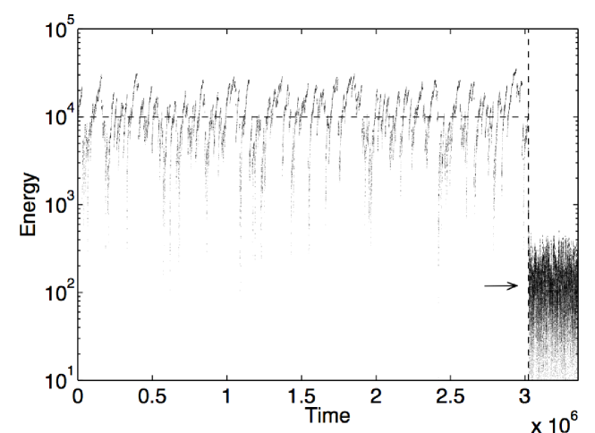
Figure 5.: A Monte Carlo simulation of Case 1 showing the system energy versus time, for the choice of parameters $\overline{\alpha}_{01}=5\times 10^{-3}$ and $\overline{\alpha}_{02}=5\times 10^{-2}$. A total of $3\times 10^{4}$ events are simulated before and after the step change. The dashed horizontal line and the arrow show the mean energies before and after the change, respectively, and the time of the change is indicated by the dashed vertical line.fig:Marko1

Figure fig:Marko2 shows an expanded view in time of the evolution of the system energy during the interval of relaxation, for the simulation shown in Figure fig:Marko1. The mean energies before and after the step change are shown by dashed horizontal lines, the time of the step change is shown by the dashed vertical line on the left, and the estimate $\overline{\tau}_{1}=1.1\times 10^{3}$ for the relaxation time is indicated by the interval between the dashed vertical lines. This figure shows the specific path $E=E(t)$ to a new steady state taken in this simulation.

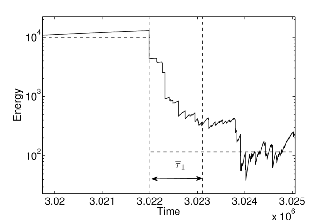
Figure 6.: An expanded view in time of the evolution of the system energy during the relaxation interval, for the simulation shown in Figure fig:Marko1. The estimate $\overline{\tau}_{1}=1.1\times 10^{3}$ for the relaxation time is indicated.fig:Marko2

Figure fig:Marko3 presents the histograms of the frequency-energy distributions (upper row) and the waiting-time distributions (lower row) for the simulation shown in Figures fig:Marko1 and fig:Marko2 before (left column) and after (right column) the step change. The frequency-energy distributions are plotted in a log-log representation, with the mean energy estimates $\overline{\cal E}_{1}=10^{4}$ and $\overline{\cal E}_{2}=10^{2}$ shown by the dashed vertical lines, and the simple power-law models for a system with a very large free energy [given by Equation (eq:ffe_tdep_bigE)] shown by the solid grey lines. The frequency-energy distributions follow the expected power laws for energies less than a rollover energy which is comparable to the mean energy estimate in each case. These results confirm the analytic arguments given in Section subsec:AnalyticTDep. The waiting-time histograms in the lower row of Figure fig:Marko3 are shown together with the simple exponential distributions corresponding to the estimates $\overline{\lambda}_{01}=0.01$ and $\overline{\lambda}_{02}=0.1$ for the mean rates of events (solid grey lines). The results show that the waiting times follow approximate exponential (Poisson) distributions, as deduced by the analytic arguments in Section subsec:AnalyticTDep. However, there is a significant discrepancy between the slope of the simulation histogram and the slope of the simple model (corresponding to the rate estimate $\overline{\lambda}_{02}=0.1$) after the change. In the simulation, the mean rates defined by the number of events divided by the elapsed time are $\overline{\lambda}_{s1}=n_{1}/\overline{t}_{1}=0.0099$ (before the change) and $\overline{\lambda}_{s2}=n_{2}/\overline{t}_{2}=0.090$ (after). The rate after the change is significantly less than the estimate given by Equation (eq:lambda_step_bigE), which indicates that the approximation $E\gg E_{c}$ is not being met. Before the change, the mean energy is approximately ${\cal E}_{1}=10^{4}E_{c}$, and Equation (eq:lambda_step_bigE) provides a good approximation. After the change ${\cal E}_{1}=10^{2}E_{c}$, and the approximation is poorer. The rate is reduced because the low system energy prevents larger flares from occurring. However, the functional form of the waiting-time distribution remains approximately exponential. The lower row in Figure fig:Marko3 also shows the simple exponential models corresponding to the mean rates $\overline{\lambda}_{s1}$ and $\overline{\lambda}_{s2}$ (dashed lines), and there is good agreement in both cases with the simulation histograms.

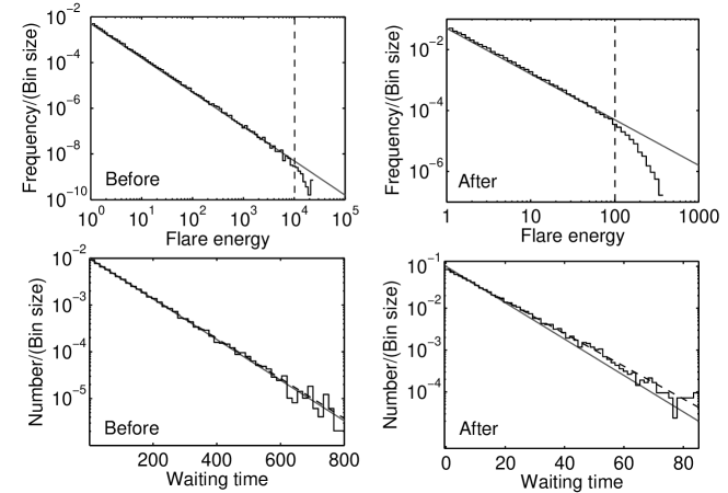
Figure 7.: Histograms representing the frequency-energy (upper row), and waiting-time (lower row) distributions before (left column) and after (right column) the step change, for the simulation shown in Figures fig:Marko1 and fig:Marko2. The dashed vertical lines in the upper row are the mean energy estimates and the solid grey curves are the power-law model for an active region with a a very large mean energy. The solid grey lines in the lower row are the the simple exponential (Poisson) models corresponding to the rates $\overline{\lambda}_{01}$ and $\overline{\lambda}_{02}$, and the dashed lines are the exponential models with rates $\overline{\lambda}_{s1}$ and $\overline{\lambda}_{s2}$ (see text).fig:Marko3

Figure fig:Marko4 illustrates part of the data from the same simulation, and is intended for qualitative comparison with the observational data for active region AR 11029, shown in Figure fig:dists_ar11029. The format of the figure is the same as Figure fig:dists_ar11029. The figure shows the events from the simulation with energy larger than $\overline{E}_{1}=10$ which occurred in the interval of time between $\overline{t}=\overline{T}-30\overline{\tau}_{1}$ and $\overline{t}=\overline{T}+10\overline{\tau}_{1}$, where $\overline{T}=3.022\times 10^{6}$ is the time of the change and $\overline{\tau}_{1}=1.1\times 10^{3}$ is the relaxation-time estimate. These choices are intended to crudely mimic observational event selection above a threshold, and to include numbers of events before and after the change which provide good statistics but which are comparable with observational numbers for the soft X-ray events. The choices give $N_{1}=341$ events in total, with $n_{11}=98$ events before the change and $n_{12}=243$ after. The upper panel in Figure fig:Marko4 shows the flare energies versus time, in the format of Figure fig:dists_ar11029. The middle panel shows the the flare cumulative number distribution for the selected events (grey diamonds), which corresponds to the frequency-energy distribution according to Equation (eq:cum_size). The black line is the simple power-law model for a system with a very large free energy, corresponding to Equation (eq:ffe_tdep_bigE). Specifically, the black line is $\overline{C}_{0}(\overline{E})=N_{1}(\overline{E}/\overline{E}_{1})^{-\gamma+1}$. The simulation events show a departure from the model $\overline{C}_{0}(\overline{E}_{1})$ at large energy due to the influence of the rollovers $\overline{\cal E}_{1}$ and $\overline{\cal E}_{2}$ (see the upper row of Figure fig:Marko3). The observed rollover for the selected events is qualitatively similar to the observations for active region AR 11029 (middle panel of Figure fig:dists_ar11029). The lower panel in Figure fig:Marko4 shows the cumulative waiting-time distribution for the selected events (grey diamonds), and the double exponential Poisson model (black curve) given by Equation (eq:wtd_pconst-poiss):

$$\ilabel{eq:sim_{t}wo_{r}ate_{m}od_{w}td}\overline{P}(\Delta\overline{t})=\frac{n_{11}}{N_{1}}\overline{\lambda}_{11}\exp(-\overline{\lambda}_{11}\Delta\overline{t})+\frac{n_{12}}{N_{1}}\overline{\lambda}_{12}\exp(-\overline{\lambda}_{12}\Delta\overline{t}),$$ (44)

where

$$\overline{\lambda}_{11}=\frac{n_{11}}{30\overline{\tau}_{1}}\quad\mbox{and}\quad\overline{\lambda}_{12}=\frac{n_{12}}{10\overline{\tau}_{1}}$$ (45)

are the rates of selected events before and after the change. This panel, which may be compared qualitatively with the lower panel in Figure fig:dists_ar11029, shows that the selected events follow the double power-law model.

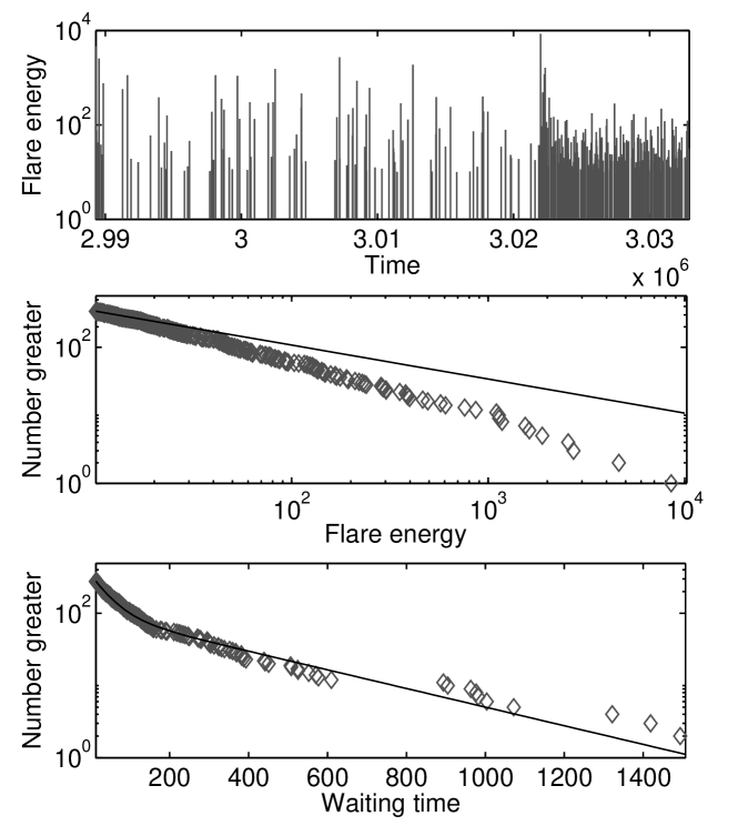
Figure 8.: Events in the simulation shown in Figures fig:Marko1-fig:Marko3 larger than size $\overline{E}_{1}=10$ which occur in the interval between 30 relaxation times before, and ten relaxation times after, the change in the rate. The format of the figure is the same as for the observational data for active region AR 11029 shown in Figure fig:dists_ar11029.fig:Marko4

Figure fig:Marko5 illustrates the relaxation process using an ensemble of 100 simulations each of $n_{2}=3\times 10^{4}$ events generated for the time after the step change. In each simulation the system is started at time $\overline{t}=0$ with energy equal to the estimate $\overline{\cal E}_{1}=10^{4}$ for the mean energy of the system before the change, and flare events are simulated for the interval of time $0\leq\overline{t}\leq 6\overline{\tau}_{1}$. These choices simulate the relaxation of the system from the steady state existing before the change in the rate. The average energy over the ensemble of 100 simulations is calculated for 600 equally spaced times during the simulation interval. Figure fig:Marko5 shows the ensemble-mean energies versus time. The estimate $\overline{\tau}_{1}=1.1\times 10^{3}$ for the relaxation time is indicated by the dashed vertical line. The average energy decreases towards the mean energy estimate $\overline{\cal E}_{2}=10^{2}$ (dashed horizontal line) following the change, reaching a statistically steady state after a time $\overline{\tau}_{\rm sim}\approx 4000-5000\approx 4\overline{\tau}_{1}$. These results suggest that the estimate $\overline{\tau}_{1}$ underestimates the actual relaxation time, which is not surprising given the large increase in the flaring rate, and hence decrease in the mean energy of the system [see comments following Equation (eq:tau2)]. This figure also indicates that the estimate for the final mean energy is an underestimate. This is also not surprising as it is an approximation, and in particular involves the assumption ${\cal E}_{2}\gg E_{c}$ [see 2008ApJ…679.1621W for the derivation].

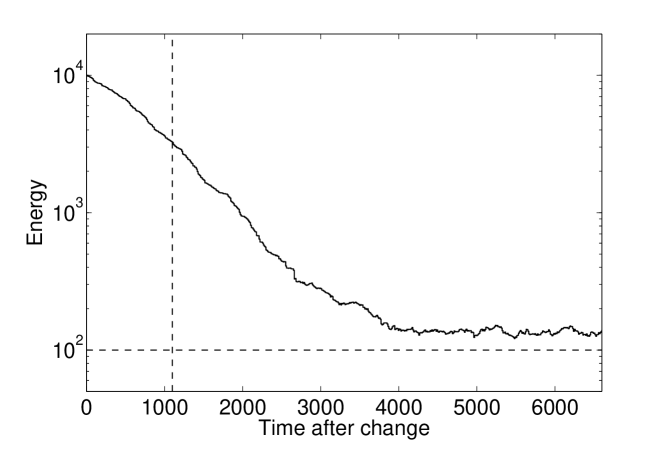
Figure 9.: An average of the energy of the system versus time over an ensemble of 100 simulations constructed for the time after the step change. The simulations start at the mean energy estimate $\overline{\cal E}_{1}=10^{4}$ for the time before the change. The estimate for the mean energy $\overline{\cal E}_{2}=10^{2}$ after the change is shown by the solid horizontal line, and the dashed vertical line is the estimate $\overline{\tau}_{1}=1.1\times 10^{3}$ for the relaxation time.fig:Marko5

4 Conclusions

sec:Conclusions

A stochastic description of the free energy of an active region, a ‘jump-transition model’ [Wheatland and Glukhov (1998), Wheatland (2008), Wheatland (2009)] is applied to model an active region which exhibits time variation in its mean flaring rate. Time variation in flare productivity is commonly observed on the Sun, for example in NOAA solar active region AR 11029, which on October 26 exhibited an approximate 10-fold increase in flaring, based on soft X-ray events compiled by the US Space Weather Prediction Center [Wheatland (2010)]. The general jump-transition model has previously been investigated only for time-independent situations, in which case it reproduces observed solar flare statistics (in particular the power-law flare frequency energy distribution, and a Poisson waiting-time distribution). The interest here is with whether the time-dependent generalization of the model also succeeds in this respect.

Time variation is incorporated in the model for two simple cases: 1. a step change in a coefficient $\alpha_{0}(t)$ describing the rates of flaring; and 2. a step change in a coefficient $\beta_{0}(t)$ describing the mean rate of energy of the system. Case 1 may be appropriate to describe solar active region AR 11029. Analytic arguments are presented that predict the qualitative behavior of the model in response to the changes. In both cases the system adjusts by shifting to a new statistically stationary steady state following the change, over a relaxation time, which is analytically estimated. Steady states of the system have mean energies which may also be analytically estimated, as shown in 1998ApJ…494..858W. Provided the mean energy is sufficiently large, the steady-state system exhibits a power-law flare frequency energy distribution (for flare energies less than a rollover value corresponding approximately to the mean energy), and exhibits simple Poisson waiting-time statistics, as shown in 2008ApJ…679.1621W and 2009SoPh..255..211W. The analytic arguments given here predict that the same is true in time-dependent situations, although the waiting-time distribution corresponds to a time-dependent Poisson process with a rate determined by the model coefficient $\alpha_{0}(t)$. For Case 1, the waiting-time distribution is in general a double exponential, corresponding to two intervals of flaring with a constant rate.

Monte Carlo simulations of the stochastic differential equation formulation of the jump transition model [Wheatland (2009)] are presented for Case 1, for parameter choices intended to qualitatively model the soft X-ray event data for active region AR 11029. The simulations confirm the analytic arguments for the behavior of the model. The observed soft X-ray flare frequency-peak flux distribution for this active region showed evidence for an upper rollover [Wheatland (2010)], which was interpreted in terms of the finite amount of energy available for flaring in a small active region being depleted by an interval of very rapid flare production. This interpretation is consistent with the the jump-transition model, and the rollover is qualitatively reproduced in the simulations presented here. A double exponential waiting-time distribution is obtained in the simulations which mimics that observed for solar active region AR 11029.

A quantitative comparison of data such as that for active region AR 11029 with the jump transition model requires estimation of flare energies, and active region energies, from the data. However, soft X-ray peak fluxes are indicative only of flare energy, and we are currently unable to reliably estimate the magnetic free energy of a solar active region [see e.g. 2009ApJ…696.1780D for an attempt to obtain energy estimates for one active region via magnetic field modeling]. Nevertheless, in future work we will consider more detailed comparison of the model with observational data.

An interesting aspect of the jump-transition model in this context is the model prediction of a departure from Poisson waiting-time statistics, if the system energy becomes sufficiently small, because large events are prevented from occurring, which reduces the overall mean rate of events. This can lead to departure from an exponential waiting-time distribution, even in the time-independent case [Wheatland (2008), Wheatland (2009)]. However, the simulations presented here reveal a new effect. If the system mean energy has intermediate values, the overall rate of events is reduced by comparison with that for a system with a large mean energy, but the waiting-time distribution remains approximately exponential. Hence the waiting-time distribution may remain exponential even when there is detailed departure from Poisson statistics. This effect was not noticed in previous modeling [Wheatland (2008), Wheatland (2009)], and also warrants further investigation. The soft X-ray events in AR 11029 appeared to follow Poisson occurrence in time based on agreement between the waiting-time distribution and the Poisson model [Wheatland (2010)]. However, the US SWPC event data suffer from significant event detection and selection problems due to the large and time varying soft X-ray background [discussed, for example, in 2001SoPh..203…87W]. Comparison with more sensitive data may be required to reveal detailed departure from Poisson occurrence.

The advent of new high resolution and high cadence short-wavelength observations of the Sun by the Advanced Imaging Assembly (AIA) on the Solar Dynamics Observatory (SDO) should enable improved investigations of solar flare event statistics, and more careful comparison with flare statistics models such as the one in this paper. The results may provide new insights into the mechanisms of energy storage and release underlying the flare phenomenon.

Acknowledgements

The authors thank Kinwah Wu for comments on a draft of the paper.

References

- Akabane (1956) Akabane, K.: 1956, PASJ, 8, 173.
- Aschwanden (2005) Aschwanden, M.J.: 2005, Physics of the Solar Corona: An Introduction with Problems and Solutions, Springer, Berlin.
- Aschwanden and McTiernan (2010) Aschwanden, M.J., McTiernan, J.M.: 2010, Astrophys. J. 717, 683.
- Barnes and Leka (2008) Barnes, G., Leka, K.D.: 2008, Astrophys. J. 688, L107.
- Benz (2008) Benz, A.O.: 2008, Living Reviews in Solar Physics 5, 1.
- Biesecker (1994) Biesecker, D.A.: 1994, Ph.D. Thesis, Univ. New Hampshire
- Boffetta et al. (1999) Boffetta, G., Carbone, V., Giuliani, P., Veltri, P., Vulpiani, A.: 1999, Phys. Rev. Lett. 83, 4662.
- Charbonneau et al. (2001) Charbonneau, P., McIntosh, S.W., Liu, H.-L., Bogdan, T.J.: 2001, Solar Phys. 203, 321.
- Chumak, Zhang, and Guo (2008) Chumak, O.V., Zhang, H.-Q., Guo, J.: 2008, Astronomy Reports 52, 852.
- Committee On The Societal & Economic Impacts Of Severe Space Weather Events (2008) Committee On The Societal, & Economic Impacts Of Severe Space Weather Events: 2008, Severe Space Weather Events: Understanding Societal and Economic Impacts Workshop Report, Space Studies Board ad hoc Committee on the Societal and Economic Impacts of Severe Space Weather Events: A Workshop, The National Academies Press, Washington DC ISBN: 978-0-309-12769-1.
- Craig (2001) Craig, I.J.D.: 2001, Solar Phys. 202, 109.
- Daly and Porporato (2007) Daly, E., Porporato, A.: 2007, Phys. Rev. E 75, 011119.
- De Rosa et al. (2009) De Rosa, M.L., Schrijver, C.J., Barnes, G., Leka, K.D., Lites, B.W., Aschwanden, M.J., Amari, T., Canou, A., McTiernan, J.M., Régnier, S., Thalmann, J.K., Valori, G., Wheatland, M.S., Wiegelmann, T., Cheung, M.C.M., Conlon, P.A., Fuhrmann, M., Inhester, B., Tadesse, T.: 2009, Astrophys. J. 696, 1780.
- Dun et al. (2007) Dun, J., Kurokawa, H., Ishii, T.T., Liu, Y., Zhang, H.: 2007, Astrophys. J. 657, 577.
- Gardiner (2004) Gardiner, C.W.: 2004, Handbook of Stochastic Methods, Springer, Berlin.
- Hudson (1991) Hudson, H.S.: 1991, Solar Phys. 133, 357.
- Hughes et al. (2003) Hughes, D., Paczuski, M., Dendy, R.O., Helander, P., McClements, K.G.: 2003, Physical Review Letters 90, 131101.
- Lepreti, Carbone, and Veltri (2001) Lepreti, F., Carbone, V., Veltri, P.: 2001, Astrophys. J. 555, L133.
- Litvinenko (1994) Litvinenko, Y.E.: 1994, Solar Phys. 151, 195.
- Lu (1995) Lu, E.T.: 1995, Astrophys. J. 447, 416.
- Lu and Hamilton (1991) Lu, E.T., Hamilton, R.J.: 1991, Astrophys. J. 380, L89.
- Lu et al. (1993) Lu, E.T., Hamilton, R.J., McTiernan, J.M., Bromund, K.R.: 1993, Astrophys. J. 412, 841.
- Moon et al. (2001) Moon, Y.-J., Choe, G.S., Yun, H.S., Park, Y.D.: 2001, J. of Geophys. Res. 106, 29951.
- Norman et al. (2001) Norman, J.P., Charbonneau, P., McIntosh, S.W., Liu, H.-L.: 2001, Astrophys. J. 557, 891.
- Odenwald, Green and Taylor (2006) Odenwald, S., Green, J., Taylor, W.: 2006, Adv. Space Res., 38, 280.
- Priest and Forbes (2002) Priest, E.R., Forbes, T.G.: 2002, Astronomy and Astrophysics Review 10, 313.
- Rosner and Vaiana (1978) Rosner, R., Vaiana, G.S.: 1978, Astrophys. J. 222, 1104.
- Scargle (1998) Scargle, J.D.: 1998, Astrophys. J. 504, 405.
- van Kampen (1992) van Kampen, N.G.: 1992, Stochastic Processes in Physics and Chemistry (Revised and enlarged edition), Elsevier Science, Amsterdam.
- Wheatland (2000) Wheatland, M. S.: 2000, ApJ, 536, L109.
- Wheatland (2001) Wheatland, M.S.: 2001, Solar Phys. 203, 87.
- Wheatland (2005) Wheatland, M.S.: 2005, Space Weather 3, 7003.
- Wheatland (2008) Wheatland, M.S.: 2008, Astrophys. J. 679, 1621.
- Wheatland (2009) Wheatland, M.S.: 2009, Solar Phys. 255, 211.
- Wheatland (2010) Wheatland, M. S.: 2010, ApJ, 710, 1324.
- Wheatland and Craig (2006) Wheatland, M.S., Craig, I.J.D.: 2006, Solar Phys. 238, 73.
- Wheatland and Glukhov (1998) Wheatland, M.S., Glukhov, S.: 1998, Astrophys. J. 494, 858.
- Wheatland and Litvinenko (2001) Wheatland, M.S., Litvinenko, Y.E.: 2001, Astrophys. J. 557, 332.
- Wheatland and Litvinenko (2002) Wheatland, M.S., Litvinenko, Y.E.: 2002, Sol. Phys., 211, 255.
- (40) Wheatland, M.S., Sturrock, P.A., McTiernan, J.M.: 1998, Astrophys. J. 509, 448.