ECCENTRICITY TRAP: TRAPPING OF RESONANTLY INTERACTING PLANETS NEAR THE DISK INNER EDGE

Abstract

Using orbital integration and analytical arguments, we have found a new mechanism (an “eccentricity trap”) to halt type I migration of planets near the inner edge of a protoplanetary disk. Because asymmetric eccentricity damping due to disk-planet interaction on the innermost planet at the disk edge plays a crucial role in the trap, this mechanism requires continuous eccentricity excitation and hence works for a resonantly interacting convoy of planets. This trap is so strong that the edge torque exerted on the innermost planet can completely halt type I migrations of many outer planets through mutual resonant perturbations. Consequently, the convoy stays outside the disk edge, as a whole. We have derived semi-analytical formula for the condition for the eccentricity trap and predict how many planets are likely to be trapped. We found that several planets or more should be trapped by this mechanism in protoplanetary disks that have cavities. It can be responsible for the formation of non-resonant, multiple, close-in super-Earth systems extending beyond 0.1AU. Such systems are being revealed by radial velocity observations to be quite common around solar-type stars.

1 INTRODUCTION

Recent radial velocity surveys indicate that a significant fraction (40–60%) of solar-type stars may harbor close-in super-Earths, with masses and periods up to $\sim 20M_{\oplus}$ and up to a few months, respectively (Mayor et al. 2009; Bouchy et al. 2009; Lo curto et al. 2010). It is suggested that in many cases, these super-Earths are members of multiple-planet systems, in which dynamical interactions may have influenced their formation although their orbits would not be in mean-motion resonances in most systems. Because mm radio observations suggest that the averaged disk mass around solar-type stars is comparable to the mass of the minimum-mass Solar nebula (Hayashi, 1981), the total mass of planetesimals would not be enough for in situ accretion of the super-Earths in the innermost regions of disks. They may have been accumulated by rocky planets that have migrated from outer regions to the proximity of the host stars. Because type I migration is halted at the inner disk edge, it may be reasonable that super-Earths accrete near the edge. If the inner disk edge is identified as accumulation locations of hot jupiters, its radius may be $\sim 0.03$–0.05AU. However, the observation suggests that averaged orbital radius of the super-Earths is $\sim 0.1$AU, well beyond the disk edge.

Ogihara & Ida (2009) performed N-body simulation to study the accretion of planets from planetesimals near the disk edge. Inward type I migration of planets is halted either by truncation of gas at the disk edge or by resonant perturbation from an inner planet. They found that in the case of relatively slow type I migration, 20–30 planets are captured by mutual mean-motion resonances and these planets start orbit crossing and giant impacts after disk gas depletion, resulting in the formation of several close-in super-Earths. The super-Earths thus formed are kicked out of resonances by strong scattering and collisions. This is in contrast to the fast migration case in which only several planets survive during the presence of the gas and they remain in stable resonant orbits even after disk gas is removed (Terquem & Papaloizou 2007; Ogihara & Ida 2009).

Ogihara & Ida (2009) also found that in the slow migration case, the innermost planet is pinned to the disk inner edge (set at $\sim 0.05$AU) and the convoy of the resonantly trapped planets extends well beyond 0.1AU. Consequently, the super-Earths which form through the giant impacts are distributed at $\sim 0.05$–0.3AU. Thus, the resultant super-Earths are multiple, non-resonant systems at $\sim 0.1$AU, which may be consistent with observed data.

A question for the result of their N-body simulation is why the resonantly trapped convoy of planets as a whole remain outside the disk edge. Because individual planets (except the innermost one) are losing angular momentum through type I migration and the angular momentum is redistributed throughout the convoy with resonant interactions, large amount of angular momentum must be supplied to prevent the planets from penetrating the disk edge. Reverse torque of type I migration near the disk edge (Masset et al., 2006) can halt planets. However, Ogihara & Ida (2009) found the trapping of a convoy outside the disk edge even in the case without the introduction of the reverse torque and the effect of the reverse torque does not change the efficiency of the trapping and orbital configurations of trapped planets.

Here, in order to investigate the trapping mechanism, we simulate in detail the orbital evolution of two planets (in some runs, more planets) with various parameters for the disk edge, the planet masses, and damping of eccentricities and semimajor axes due to disk-planet interactions. Together with analytical arguments, we find that asymmetric damping of eccentricity of the innermost planet near the disk edge is responsible for angular momentum input from the disk to the planet with such a high rate that it compensates for the angular momentum loss of all the trapped planets due to inward type I migration. We call this trapping mechanism an “eccentricity trap.”

Although the eccentricity trap does not occur for some parameter values of the disk and planets, once the eccentricity trap occurs, it may be stronger than the trap by the reverse type I torque. We derive semi-analytical formula for the conditions necessary to produce an eccentricity trap, as a function of planet masses, eccentricity and semimajor axis damping timescales, and disk edge width. We also predict how many planets can be trapped. For likely parameter values for the innermost regions in protoplanetary disks, the condition for an eccentricity trap may be satisfied, while some systems including our solar system might not have had a clear inner cavity in the disk and therefore lost the inner planets.

In section 2, we present analytical argument to clearly show the intrinsic physics of the eccentricity trap. In section 3, we show the results of N-body simulations. Comparing analytical arguments and the numerical results, we derive quantitative conditions for the occurrence of the eccentricity trap. In section 4, we summarize the results and discuss their implications.

2 ECCENTRICITY TRAP

2.1 Basic Idea

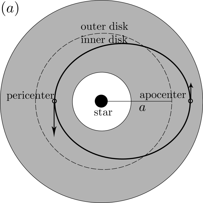
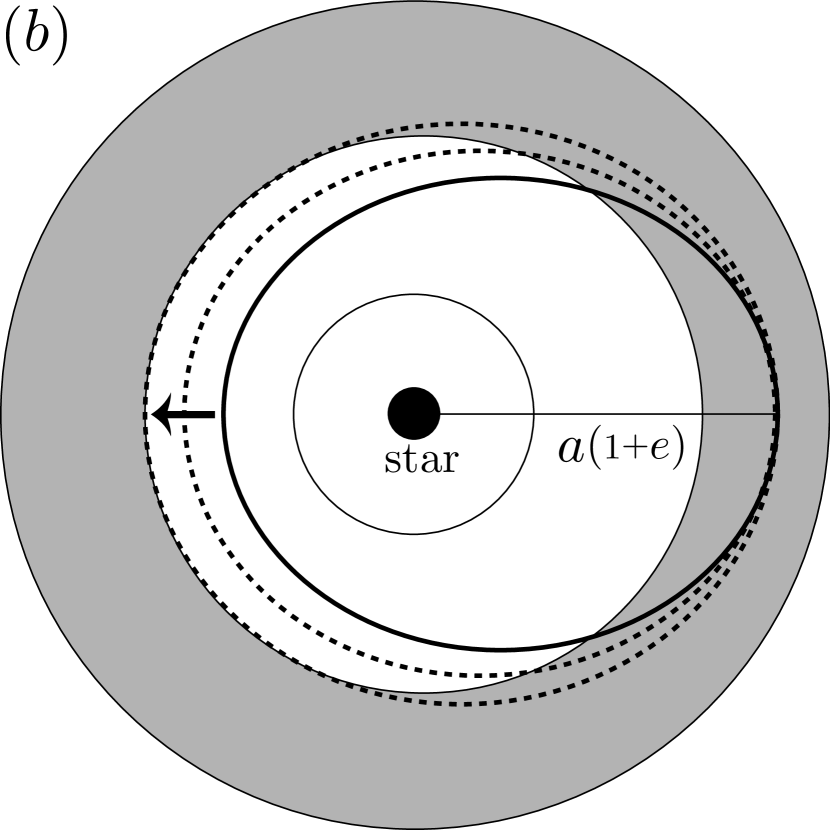
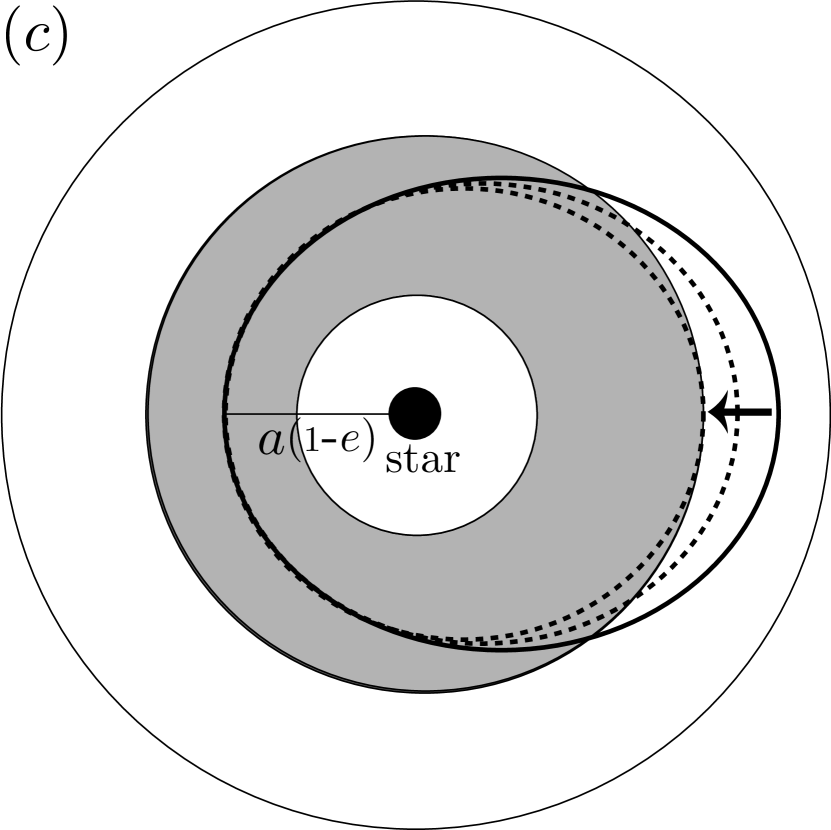
Figure 1: Schematic illustration of expansion/shrink of $a$ due to $e$-damping. (a) The solid line represents an eccentric orbit with semimajor axis $a$ around a star. The shaded toroidal region represents a gas disk. The guiding center, which divides the disk into two areas, is expressed by the dashed line. At apocenter, the tangential velocity of the planet is slower than the local gas velocity, while the orbital velocity is faster than the gas velocity at pericenter. (b) The planet suffers a tailwind when it is moving in the outer disk, which increases $a$ while decreases $e$ with the apocenter $a(1+e)$ kept almost constant. (c) In the inner disk region, the planet suffers a headwind, leading to a decrease of $a$, with the pericenter $a(1-e)$ kept almost constant.

Consider a planet in an orbit with eccentricity $e$ and semimajor axis $a$ in a gas disk (Fig. 1a). We now consider changes in $a$ and $e$ caused by gravitational drag (dynamical friction) from disk gas (Ostriker 1999, Tanaka & Ward 2004; for details, see section 2.2). The tangential velocity of the planet near the apocenter in an eccentric orbit is slower than local circular Keplerian velocity when the planet moves through an outer disk region. Since the gas velocity is almost equal to circular Keplerian velocity, the planet suffers a tailwind. Then, $a$ increases while $e$ decreases, in such a way that $a(1+e)$ is almost kept constant (see schematic illustration in Fig. 1b). On the other hand, the planet suffers a headwind when it moves through an inner disk region. Then, both $e$ and $a$ decrease such that $a(1-e)$ is almost kept constant (Fig. 1c). Thus, $e$ is decreased by interactions with both outer and inner disks, while changes in $a$ due to the the outer and inner disks cancel out.

If the planet has an eccentric orbit that straddles a relatively sharp disk edge inside which disk gas is depleted to create a cavity, it suffers a drag force only when it moves in the outer disk region, so that $e$ decreases and $a$ increases on orbit average. Since the specific angular momentum of the planet is

$$L=\sqrt{GM_{*}a(1-e^{2})},$$ (1)

where $M_{*}$ is the host star mass, the planet apparently gains orbital angular momentum through gas drag.

Note that type I migration torque decreases $a$ even in the case of a circular orbit (e.g., Ward 1986, Tanaka et al. 2002). In that case, the planet loses $L$ mostly by distant perturbations from the outer disk and gains $L$ by those from the inner disk. The loss and gain are almost balanced, but the effects of curvature of the system and negative pressure radial gradient slightly enhance the loss, resulting in net inward migration (type I migration). Because type I migration is caused by residual of opposing torques while the $e$-damping does not have such cancellation, the timescale of type I migration ($t_{a}$) is usually much longer than the $e$-damping timescale ($t_{e}$) (see section 3.1).

Since the $a$-increase by the edge effect occurs on a timescale $\sim t_{e}$, the angular momentum gain rate due to the edge effect is much higher than the angular momentum loss rate due to type I migration unless $e$ is extremely small (see Eq. [18]). Therefore, if the planet migrates inward due to type I migration, it should be “trapped” at the disk edge, as long as orbital eccentricity is maintained to some level. If another planet migrates to be trapped in a mean-motion resonance with the inner planet trapped at the edge, the resonant perturbations from the outer planet continuously pump up eccentricity of the inner one and it enables the eccentricity trap to be maintained. Usually other planets also migrate inward and are captured at mutual mean-motion resonances one after another to form a convoy of planets. Since the angular momentum gain due to the edge effect is significant, it can compensate for the total loss of several planets due to type I migration and trap the convoy of planets as a whole outside the edge.

2.2 Condition for the Trapping

In this subsection, we derive an approximate condition for the eccentricity trap, in order to understand the results of N-body simulations in section 3. Since in the N-body simulations, we integrate orbits by adding the instantaneous drag forces derived by Tanaka & Ward (2004) to the equations of motion (rather than secularly changing the orbital elements with orbit-averaged torques), we derive the trap condition using their force formulas.

Goldreich & Tremaine (1980), Ward (1988), and Artymowicz (1993) derived the damping rate of $e$ due to planet-disk interactions. They summed up resonances to obtain an orbit-averaged $e$-damping rate, assuming uniformity of disk gas density on a scale of radial excursion of the planet. In the situation we are considering, however, gas density that a planet passes through significantly changes during an orbital period, so that we cannot apply their orbit-averaged results. Derivation of the formulas for the torque exerted on a planet in an eccentric orbit straddling a disk edge, based on full descriptions of Lindblad and corotation resonances, is left for future work.

On the other hand, Tanaka & Ward (2004) derived instantaneous drag forces caused by gravitational potential perturbations due to density waves at each point of epicycle motion of the planet. They showed that the mean $e$-damping rate (Eq. [5]) obtained by averaging the instantaneous forces over one orbital period agrees with that predicted by summing up resonant torques in the case of locally uniform gas density. Ostriker (1999) calculated dynamical friction from gas flow onto a particle. Since gas density is higher in downstream than in upstream due to gravitational focusing, the particle is pulled back by the gravity of the higher gas density, which is similar to Chandrasekahr’s dynamical friction in a stellar cluster (Binney & Tremaine, 1987). Tanaka & Ward (2004) also showed that spiral waves are always stronger in backside of the epicycle motion (Fig. 1 in their paper). The Ostriker’s force formula agrees with Tanaka & Ward’s one except for a numerical factor.

Because the force formulas by Tanaka & Ward (2004) are local expressions, we adopt them both in N-body simulations and analytic arguments in this paper (see cautions below). In the N-body simulations, the forces are directly included in equations of motion. The formulas for the specific damping forces are:

$$\textit{F}_{{\rm damp},r} = \frac{1}{0.78t_{e}}(2A^{c}_{r}[v_{\theta}-r\Omega]+A^{s}_{r}v_{r})$$ (2)

$$\textit{F}_{{\rm damp},\theta} = \frac{1}{0.78t_{e}}(2A^{c}_{\theta}[v_{\theta}-r\Omega]+A^{s}_{\theta}v_{r})$$ (3)

$$\textit{F}_{{\rm damp},z} = \frac{1}{0.78t_{e}}(A^{c}_{z}v_{z}+A^{s}_{z}z\Omega)$$ (4)

where $v_{r},v_{\theta}$, and $v_{z}$ are radial, tangential, and vertical components of the planet’s velocity, $r\Omega$ is circular velocity of disk gas, which is almost equal to local Keplerian velocity, and the numerical factors are given by

$$A^{c}_{r}=0.057 A^{s}_{r}=0.176$$

$$A^{c}_{\theta}=-0.868 A^{s}_{\theta}=0.325$$

$$A^{c}_{z}=-1.088 A^{s}_{z}=-0.871.$$

In the case of locally uniform gas density, integrating $\textit{F}_{{\rm damp},r}$ and $\textit{F}_{{\rm damp},\theta}$ over one orbital period, Tanaka & Ward (2004) derived the averaged $e$-damping timescale ($t_{e}$),

$$t_{e}=\frac{e}{\dot{e}}=\frac{1}{0.78}\left(\frac{M}{M_{*}}\right)^{-1}\left(\frac{\Sigma_{g}r^{2}}{M_{*}}\right)^{-1}\left(\frac{c_{s}}{v_{\rm K}}\right)^{4}\Omega^{-1},$$ (5)

where $M$ and $M_{*}$ are masses of the planet and the host star, and $\Sigma_{g}$ and $c_{s}$ are the gas surface density and the sound velocity of the disk gas, respectively.

These Tanaka & Ward’s formulas assumed subsonic flow. We apply the formulas even for supersonic cases in which radial excursion is wider than the disk edge width that may be comparable to disk scale height ($H$). Ostriker (1999) showed that the formula of the drag force must be multiplied by a correction factor, $1/(1+(v/c_{s})^{3})$, in the case of supersonic flow. The correction factor is consistent with a supersonic correction factor for an averaged $e$-damping rate derived by Papaloizou & Larwood (2000), if the relative velocity $v$ is identified by $ev_{\rm K}$. We also carried out simulations with the correction factor (section 3.4). Tanaka & Ward’s formulas also assumed that gas density is locally uniform on spatial scale of $\sim H$. We apply the formulas also for the regions near the disk edge in which gas density may vary on a scale of $\sim H$. The detailed analysis of its validity is left for future work, because the purpose of the present paper is to demonstrate a potential importance of the eccentricity trap that we firstly found.

The edge effect described in section 2.1 is quantitatively estimated with local (Hill) approximation, as follows. In the Hill coordinates that are comoving with the planet’s guiding center at $a$, the tangential velocity of the planet at $r=a+x=a(1+e\cos(\Omega_{0}t))$ is

$$v_{y}=-2ea\Omega_{0}\cos(\Omega_{0}t)=-2x\Omega_{0},$$ (6)

where $\Omega_{0}=\sqrt{GM_{*}/a^{3}}$. The Keplerian shear velocity (the local Keplerian circular velocity in the Hill coordinates) of gas at $x$ is

$$v_{\rm shear}=-\frac{3}{2}x\Omega_{0}.$$ (7)

The tangential relative velocity between the planet and local disk gas is

$$\Delta v=v_{\theta}-r\Omega=v_{y}-v_{\rm shear}=-\frac{1}{2}x\Omega_{0}.$$ (8)

Since the planet always moves slower than the gas ($\Delta v<0$) at $x>0$, the drag force accelerates the planet’s rotation there. At apocenter, the above expression is also easily found in global coordinates. The tangential velocity of the planet at the apocenter in the inertial frame is

$$v_{\theta,{\rm apo}}=\frac{L}{a(1+e)}=\sqrt{\frac{GM_{*}(1-e)}{a(1+e)}},$$ (9)

where $L$ is specific angular momentum of the planet ($L=\sqrt{GM_{*}a(1-e^{2})}$), while the local circular Keplerian velocity is

$$v_{\rm K,apo}=\sqrt{\frac{GM_{*}}{a(1+e)}}.$$ (10)

Hence, for $e\ll 1$,

$$\Delta v=v_{\theta,{\rm apo}}-v_{\rm K,apo}\simeq-\frac{1}{2}ea\Omega_{0},$$ (11)

which is identical to Eq. (8) at the apocenter ($x=ea$).

If the disk edge width is sharp enough ($ea\gg\Delta r$) and the edge is at $x\simeq 0$, the torque due to gravitational drag operates only at $x>0$, then the torque due to the $e$-damping averaged over Keplerian time ($T_{\rm K}=2\pi/\Omega_{0}$), which we call “edge torque,” is

$$N_{\rm edge}\simeq\frac{1}{T_{\rm K}}\int_{-T_{\rm K}/4}^{T_{\rm K}/4}MrF_{{\rm damp},\theta}dt,$$ (12)

where $M$ is the planet mass. Since $v_{\theta}-r\Omega=(ae/2)\Omega_{0}\cos(\Omega_{0}t)$ and $v_{r}=ae\Omega_{0}\sin(\Omega_{0}t)$, Eq. (3) becomes

$$F_{{\rm damp},\theta}=\frac{ae\Omega_{0}}{0.78t_{e}}\left(-A_{\theta}^{c}\cos(\Omega_{0}t)+A_{\theta}^{s}\sin(\Omega_{0}t)\right).$$ (13)

Then, Eq. (12) is reduced to

$$N_{\rm edge}\simeq-\frac{M}{T_{\rm K}}\int_{-T_{\rm K}/4}^{T_{\rm K}/4}\frac{A_{\theta}^{c}}{0.78}\frac{ea\Omega_{0}\cos(\Omega_{0}t)}{2t_{e}}adt\simeq\frac{M}{2\pi}\frac{ea^{2}\Omega_{0}}{t_{e}}\simeq\frac{eML}{2\pi t_{e}}\;\;\left(=\frac{N_{e,{\rm apo}}}{\pi}\right),$$ (14)

where $N_{e,{\rm apo}}$ is the torque at the apocenter ($N_{e,{\rm apo}}\simeq eMa^{2}\Omega_{0}/2t_{e}$).

If $\Delta r\gg ea$, the planet suffers an opposing torque at $x<0$ and the net torque must almost vanish on orbit average. (In other words, with the integral range from $-T_{\rm K}/2$ to $T_{\rm K}/2$, the above integral vanishes.) Thus, in general cases, the edge torque can be expressed with a reduction factor $f$ $(0<f<1)$, which is a function of $ea/\Delta r$, as

$$N_{\rm edge}\simeq f\frac{eML}{2\pi t_{e}}.$$ (15)

If the edge is at $x>0$, the range of integral in Eq. (14) is $-t_{\rm int}$ to $t_{\rm int}$ with $t_{\rm int}<T_{\rm K}/4$. If the edge is at $x<0$, $t_{\rm int}>T_{\rm K}/4$. In either case, the integrated value is smaller than that in Eq. (14), which means that Eq. (15) is the maximum value of $N_{\rm edge}$.

In our N-body simulation, even for planets near the edge, we apply the conventional inward migration with a timescale given by (Tanaka et al., 2002)

$$t_{a}=-\frac{a}{\dot{a}}=\frac{1}{2.7+1.1q}\left(\frac{M}{M_{*}}\right)^{-1}\left(\frac{\Sigma_{g}r^{2}}{M_{*}}\right)^{-1}\left(\frac{c_{s}}{v_{\rm K}}\right)^{2}\Omega^{-1},$$ (16)

where $\Sigma_{g}\propto r^{-q}$. Masset et al. (2006) pointed out that near the disk edge, due to the local positive surface density gradient, the migration may be reversed to be outward. The radiative effect can also make the migration outward in optically thick disks (e.g., Paardekooper et al. 2010; Lyra et al. 2010). Furthermore, Papaloizou & Larwood (2000) suggested that migration is slowed and reversed in supersonic cases (the migration timescale has an additional factor of $(1+(ev_{\rm K}/c_{s})^{5})/(1-(ev_{\rm K}/c_{s})^{4})$). Thus, our prescription for type I migration underestimates the efficiency of the trapping at the edge. Nevertheless, our N-body simulation shows that the eccentricity trap does occur. The effects of the local positive surface density gradient at the disk edge and radiation are left to future work.

In the equilibrium state of the trapping, the edge torque is balanced with the sum of the type I migration torque on the planet at the edge and the resonant torque from an outer perturber ($-N_{p}$). As we assume a conventional type I migration at the edge, the type I migration torque on the innermost planet is given by $-ML/2t_{a}$. Therefore, the condition for the planet to be trapped at the edge is

$$\frac{fe}{2\pi}\frac{ML}{t_{e}}-\frac{ML}{2t_{a}}-N_{p}>0.$$ (17)

We first consider the simplest case of two equal-mass ($M$) planets. In this case, the gravitational torque by the inner planet on the outer planet, $-N_{p}$, balances the type I migration torque on the outer planet given by $N_{p}\simeq ML/2t_{a}$. Then, Eq. (17) becomes

$$\frac{t_{e}}{t_{a}}<\frac{fe}{2\pi}.$$ (18)

Here, we assume that difference in semimajor axes of inner and outer planets is small enough and represent them as a mean value, $a$, in Eq. (18) for simplicity. Thereby, although we consider trapping at the edge, the trapping condition is reduced to that parameterized by the orbit-averaged damping timescales of $e$ and $a$ in uniform gas ($t_{e}$ and $t_{a}$).

3 NUMERICAL SIMULATION

3.1 Comparison between Theory and Simulation

The above trapping mechanism is quantitatively well demonstrated by simple two-planet systems in which the inner planet is located at a sharp disk edge. We have calculated the orbital evolution of two planets including effects of type I migration, gravitational drag, and the disk edge. The orbits of the planets are integrated by a 4th order Hermite scheme, adding instantaneous drag forces Eqs. (2), (3), and (4) corresponding to $e$-damping and a tangential force,

$$\textit{F}_{{\rm mig},\theta}=\frac{v_{\rm K}}{2t_{a}},$$ (19)

corresponding to $a$-damping, following Ogihara & Ida (2009).

The parameters in the trapping condition (Eq. [18]) are $t_{e}/t_{a}$ and $\Delta r/r_{\rm edge}$, where $r_{\rm edge}$ is the location of the disk edge. If $\Delta r$ is comparable to the disk scale height ($H$),

$$\frac{\Delta r}{r_{\rm edge}}\simeq\frac{c_{s}}{v_{\rm K}}.$$ (20)

(Note that the disk edge may be truncated by stellar magnetic field and $\Delta r$ is not necessarily $\sim H$.) From Eqs. (5) and (16),

$$\frac{t_{e}}{t_{a}}=\frac{2.7+1.1q}{0.78}\left(\frac{c_{s}}{v_{\rm K}}\right)^{2}\ll 1.$$ (21)

At $r\sim 0.05$AU corresponding to the inner disk edge, $T\simeq 1250$K in the optically thin limit (Hayashi, 1981). Since $v_{\rm K}\simeq 130(r/0.05{\rm AU})^{-1/2}$km/s and $c_{s}\simeq 2(T/1250{\rm K})^{1/2}$km/s, $c_{s}/v_{\rm K}\simeq 0.016$ at $r\sim 0.05$AU. In an optically thick disk, $T$ can be higher. However, since silicate dust grains sublimate and the disk becomes optically thin at $T\gtrsim 1400$K, $T$ cannot be higher than that. On the other hand, $t_{a}$ can be longer due to non-linear effects. Hence, at $r\sim 0.05$AU, $t_{e}/t_{a}\simeq 10^{-4}$–$10^{-3}$ and $t_{e}\sim 100T_{\rm K}$ for $M=M_{\oplus}$. We perform calculations with wide ranges of $\Delta r/r_{\rm edge}$ and $t_{e}/t_{a}$ with fiducial values of $\Delta r/r_{\rm edge}=0.01$ and $t_{e}/t_{a}=10^{-3}$. In all runs, $t_{e}/T_{\rm K}=100$ and $q=1.5$ are used, and the gas surface density vanishes with a hyperbolic tangent function of width $\Delta r$.

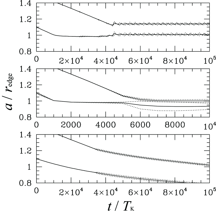
Figure 2: Orbital evolution of the planets. Solid lines are semimajor axes, and dotted lines are apocenters and pericenters. Top: The result of the fiducial case with $\Delta r/r_{\rm edge}=0.01$ and $t_{e}/t_{a}=10^{-3}.$ Middle: The result of a fast migration case with $t_{e}/t_{a}=10^{-2}$. Bottom: The result of a smooth edge case with $\Delta r/r_{\rm edge}=0.2$.

The results of the orbital integrations are presented in Figure 2. Two planets with Earth mass $M_{\oplus}$ are initially placed in almost circular orbits. The top panel shows the orbital evolution of the fiducial case with $\Delta r/r_{\rm edge}=0.01$ and $t_{e}/t_{a}=10^{-3}$. The solid lines represent the semimajor axis $a$, and the dotted lines represent the pericenters $a(1-e)$ and apocenters $a(1+e)$. The inner planet migrates to the edge and stays there because $\Sigma_{g}$ vanishes and $t_{a}\rightarrow\infty$ there. After that, the outer planet migrates to be trapped in the 6:5 mean-motion resonance with the inner one. Once the planets are captured in the resonance (at $t\sim 45000T_{\rm K}$), the eccentricities of both planets are pumped up to $e\sim 0.01$ and their $a$’s are shifted slightly outward, resulting in an eccentricity trap.

The eccentricity trap depends on the parameter values. The middle panel shows the result of fast migration cases with $t_{e}/t_{a}=10^{-2}$ ($\Delta r/r_{\rm edge}=0.01$). The planets are not trapped at the edge since the type I migration speed is too fast in this case, although the eccentricities become about 0.06 at the moment of capture into a resonance. The bottom panel shows the result of smooth edge case of $\Delta r/r_{\rm edge}=0.2$ ($t_{e}/t_{a}=10^{-3}$). The planets also penetrate into the cavity because the edge effect is weak.

We now derive a trapping condition by using the simulation results. We calculated a torque due to the gas drag at each timestep in the orbital integration and found that the orbit-averaged torque is well fitted with

$$f\simeq\left\{\begin{array}[]{ll}1&(\mbox{for }er_{\rm edge}>\Delta r)\\ {\displaystyle\sqrt{\frac{er_{\rm edge}}{\Delta r}}}&(\mbox{for }er_{\rm edge}<\Delta r).\end{array}\right.$$ (22)

In the fiducial case with $\Delta r=0.01r_{\rm edge}$, we found that $e\sim 0.01$, so that $f\simeq 1$.

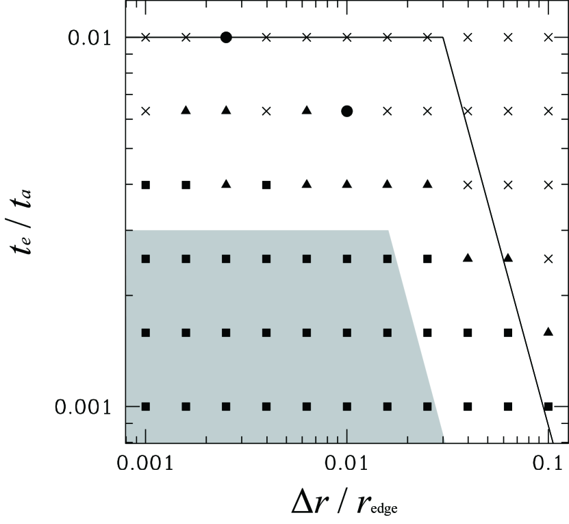
Figure 3: The results of trapping for various values of $\Delta r/r_{\rm edge}$ and $t_{e}/t_{a}$. Crosses indicate that planets are not trapped, while other filled symbols indicate that planets are trapped. The filled squares, triangles, and circles represent the time-averaged eccentricity $e<0.02,0.02<e<0.03$, and $e>0.03$, respectively. The shaded region represents the theoretically predicted trapping regions (Eq. [26]). The solid line represents the upper limit (necessary condition) for the eccentricity trap.

The results with various $t_{e}/t_{a}$ and $\Delta r/r_{\rm edge}$ for two Earth-mass planets are summarized in Fig. 3. Crosses represent the cases in which planets are not trapped. Other symbols represent the trapped cases. The filled squares, triangles, and circles represent the time-averaged eccentricity of the inner planet of $e<0.02$, $0.02<e<0.03$, and $e>0.03$, respectively.

In order to compare the semi-analytical condition, Eq. (18), with the orbital integration results, we need a formula for resonantly excited eccentricities. We must also take into account the dependence on planetary masses. Let $M_{1}$ and $M_{2}$ be the masses of the inner and outer planets, respectively. The eccentricity of the inner planet after resonant trapping is expressed in the Hill approximation (e.g., Nakazawa & Ida 1988) as

$$e\sim e_{\rm res}\frac{M_{2}}{M_{1}+M_{2}}\equiv e_{\rm res}\frac{\nu_{2}}{2},$$ (23)

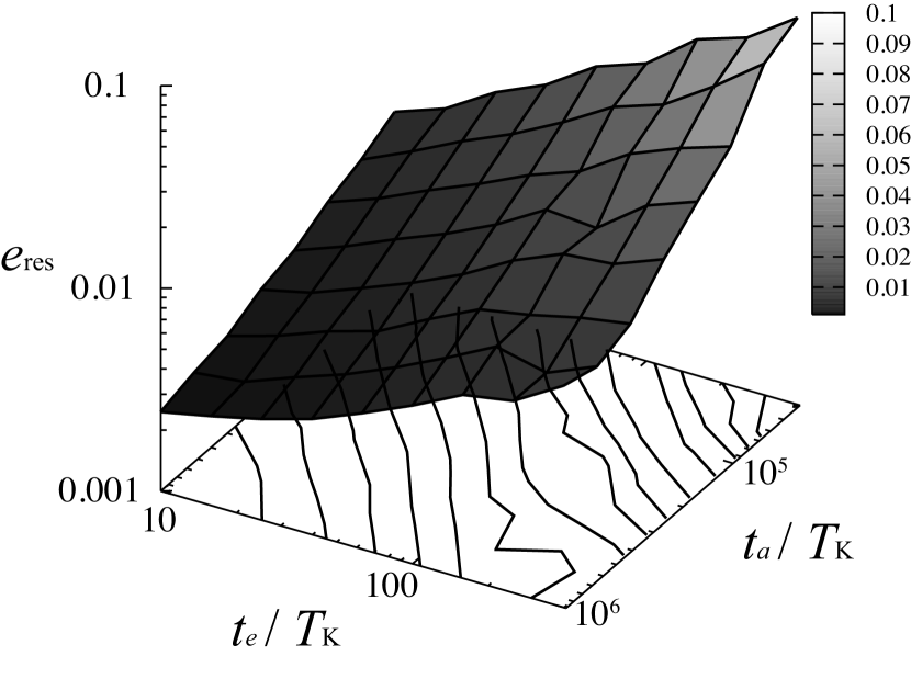
Figure 4: The relative eccentricity excited by resonant trapping is plotted against $t_{e}$ and $t_{a}$ through numerical simulations. In these calculations, $M_{1}=M_{2}=M_{\oplus}$ is assumed. The contours are drawn from $e_{\rm res}=10^{-2.5}$ to $10^{-1.2}$ with intervals $\Delta\log_{10}e_{\rm res}=$ 0.1.

where $e_{\rm res}$ is the eccentricity of the relative motion (In the Hill approximation, relative motion between two Keplerian motions is another Keplerian motion). Since the magnitude of the relative eccentricity excited by resonant interaction ($e_{\rm res}$) with damping is not theoretically clear, we use empirical values. With $M_{1}=M_{2}=M_{\oplus}$, we have done the same calculations as Fig. 3 for various values of $t_{e}$ [$=(10$–$10^{3})T_{\rm K}$] and $t_{a}$ [$=(10^{4}$–$10^{6})T_{\rm K}$]. In Figure 4, $e_{\rm res}$ is plotted against $t_{e}$ and $t_{a}$. The relative eccentricity can be fitted by

$$e_{\rm res}\simeq 0.02\left(\frac{t_{e}/t_{a}}{10^{-3}}\right)^{1/2}.$$ (24)

The trapping condition for a given mean-motion resonance may be $t_{\rm lib}<t_{a}$, where $t_{\rm lib}$ is the libration timescale of the eccentricity by the secular perturbation,

$$t_{\rm lib}\sim\left(\frac{\mu}{M_{*}}\right)^{-1}\left(\frac{a_{2}}{a_{1}}\right)^{3}T_{\rm K},$$ (25)

where $\mu=M_{1}M_{2}/(M_{1}+M_{2})$ is the reduced mass, $M_{1}$ and $M_{2}$ are masses of the inner and outer planets, and $a_{1}$ and $a_{2}$ are their semimajor axes (e.g., Murray & Dermott 1999). Since $t_{\rm lib}$ is larger for larger $a_{2}/a_{1}$, the planets tend to be trapped by a more distant resonance for larger $t_{a}$. As a result, $e_{\rm res}$ is smaller. In section 3.2, we will show through calculations with $M_{1}=M_{2}=(0.1$–$10)M_{\oplus}$ that the magnitude of $e_{\rm res}$ is almost independent of the planetary mass in the trapped case as long as $t_{e}/t_{a}$ is fixed. The fact that all of $t_{\rm lib}$, $t_{e}$ and $t_{a}$ are inversely proportional to planetary mass suggests that the resonance at which planets are trapped and hence the values of $e_{\rm res}$ would not sensitively depend on planetary masses. However, note that the formula (Eq. [24]) is empirical and can strictly be applied only for the range of parameters that we tested.

Substituting $e=e_{\rm res}/2$ into Eq. (18), the trapping condition is reduced to

$$\frac{t_{e}}{t_{a}}\lesssim\left\{\begin{array}[]{ll}0.003\nu_{2}^{2}&\mbox{for }\Delta r/r_{\rm edge}<0.017\nu_{2}^{2},\\ {\displaystyle 0.008\nu_{2}^{6}\left(\frac{\Delta r/r_{\rm edge}}{0.01}\right)^{-2}}&\mbox{for }\Delta r/r_{\rm edge}>0.017\nu_{2}^{2},\end{array}\right.$$ (26)

where $\nu_{2}=2M_{2}/(M_{1}+M_{2})$ and $\nu_{2}=1$ for equal-mass planets. The shaded region in Fig. 3 represents the above semi-analytical trapping condition, which is approximately consistent with the numerical results of orbital integrations. Note that in N-body simulations, the magnitude of the type I migration torque on the innermost planet should be smaller than $ML/2t_{a}$ (which is adopted in Eq. [17]) because the innermost planet is located near the edge where gas density is smaller. Accordingly, the trapping region would be larger than the shaded region. On the other hand, neglecting the type I migration torque on the innermost planet in Eq.(17), we obtain the necessary condition for trapping (solid line in Fig. 3). The transition from the trapping and non-trapping should occur in the region between the outer boundary of the shaded region and the solid line, which is consistent with the numerical results. Thus, the condition Eq. (18) is a slightly conservative condition. Since the semi-analytical condition includes planetary mass dependence through $\nu_{2}$, we next examine it by comparing orbital integrations and the semi-analytical argument.

3.2 Dependence on Planetary Mass

The dependence of trapping condition on the planetary mass is investigated in this subsection. Let $M_{1}$ and $M_{2}$ be masses of the inner and outer planets. As in the discussion on Eq. (17), we represent their semimajor axes ($a_{1}$ and $a_{2}$) as a mean value, $a$ $(\sim a_{1},a_{2})$, for simplicity. In this case, Eq. (17) is

$$\frac{fe_{1}}{2\pi}\frac{M_{1}L}{t_{e}(M_{1})}-\frac{M_{1}L}{2t_{a}(M_{1})}-N_{p}>0,$$ (27)

where

$$N_{p}=-\frac{M_{2}L(a_{2})}{2t_{a}(M_{2},a_{2})}=-\frac{M_{1}L(a_{1})}{2t_{a}(M_{1},a_{1})}\left(\frac{a_{2}}{a_{1}}\right)^{-q+1/2}\left(\frac{M_{2}}{M_{1}}\right)^{2}\simeq-\frac{M_{1}L}{2t_{a}(M_{1})}\left(\frac{M_{2}}{M_{1}}\right)^{2}.$$ (28)

With Eq. (24), the trapping condition is given by

$$\frac{(M_{1}^{2}+M_{2}^{2})(M_{1}+M_{2})}{M_{1}^{2}M_{2}}<C,$$ (29)

where

$$C=\frac{e_{\rm res}f}{\pi}\frac{t_{a}}{t_{e}}=\frac{20f}{\pi}\left(\frac{t_{e}/t_{a}}{10^{-3}}\right)^{-1/2}.$$ (30)

For a fiducial case with $t_{e}/t_{a}=10^{-3}$ and $\Delta r/r_{\rm edge}=0.01$, $e_{\rm res}\simeq 0.02$ and $f\simeq 1$, so that $C\simeq 6$.

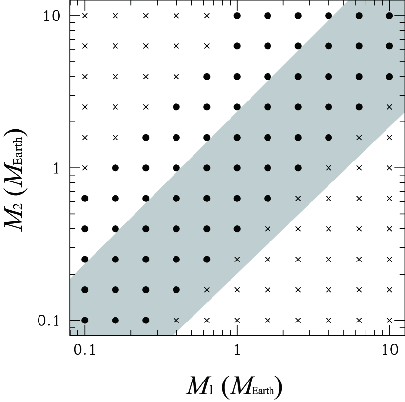
Figure 5: The results of trapping for various masses of inner and outer planets ($M_{1}$, $M_{2}$). Filled circles represent the cases where planets are trapped, while crosses represent non-trapped cases. The shaded region represents the theoretically predicted trapping regions given by Eq. (29).

To confirm the above condition, we carried out additional numerical simulations with various planetary masses, (0.1–$10)M_{\oplus}$. We used the fiducial parameters, $t_{e}/t_{a}=10^{-3}$ and $\Delta r/r_{\rm edge}=0.01$. Since the $e$-damping time is set such that $t_{e}=100(M/M_{\oplus})^{-1}T_{\rm K}$, in order to keep $t_{a}/t_{\rm lib}$ constant, we found that the resonance at which planets are trapped is similar and $e_{\rm res}\sim 0.02$ in most of the trapped cases even if $M_{1}$ and $M_{2}$ are changed from $0.1M_{\oplus}$ to $10M_{\oplus}$. Note that $e_{\rm res}$ becomes larger than 0.02 when $M_{2}\sim CM_{1}>M_{1}$. Figure 5 summarizes the results on the $M_{1}-M_{2}$ plane. The trapped and non-trapped cases are indicated by filled circles and crosses, respectively. The shaded region represents the trapping condition (Eq. [29]). The results are consistent with the analytical condition except that the trapping is more extended to high $M_{2}/M_{1}$ regions, because N-body simulations show higher $e_{\rm res}$ than that assumed in the analytical estimate in the high $M_{2}/M_{1}$ regions.

The results might seem rather counter-intuitive. That is, the trap does not occur when the outer planet is very small, while the trap does occur even if the outer planet is somewhat more massive than the inner one. If the outer planet is too small, the excited magnitude of $e_{1}$ is too small for the edge torque to be effective. On the other hand, even if the outer planet is more massive, the trapping can occur, because $e_{1}$ is excited highly enough. For a further massive outer planet, the edge torque is no more balanced with angular momentum loss due to type I migration of the massive outer planet. Thus, the eccentricity trap works for planets with comparable masses, which is often the case during planet formation, because planets actually start migration when migration timescale ($\propto M^{-1}$) becomes shorter than growth timescale ($\propto M^{1/3}$) and hence the migrating planets should have similar masses.

3.3 Number of Trapped Bodies

We also investigated systems with more than two planets. The trapping condition becomes more severe than in two planet systems, since the edge torque on the innermost planet must balance the type I migration torques of all the planets. The number of planets that can be trapped by the edge effect increases with increase in the type I migration timescale. In fact, Ogihara & Ida (2009) found that 20–30 planetary embryos are lined up by the edge effect in the case of slow migration.

We estimate the maximum number of trapped planets. For simplicity, we assume equal mass bodies. When $n$ planets are trapped near the disk edge, Eq. (28) is replaced by

$$N_{p}\sim-\frac{n-1}{2t_{a}}ML,$$ (31)

where we also neglected the $a$-dependence, although it may not be able to neglected for sufficiently large $n$. Then, Eq. (17) becomes

$$\frac{fe_{\rm res}}{4\pi}\frac{1}{t_{e}}-\frac{1}{2t_{a}}-\frac{n-1}{2t_{a}}>0.$$ (32)

Therefore,

$$n<\frac{fe_{\rm res}}{2\pi}\frac{t_{a}}{t_{e}}.$$ (33)

Through N-body simulation, we also derived the dependence of $n$ on $e_{\rm res}$ (Eq. [24]) as

$$e_{\rm res}\simeq 0.02\left(\frac{t_{e}/t_{a}}{10^{-3}}\right)^{1/2}\left(\frac{n}{2}\right)^{1/2}.$$ (34)

Then, Equation (33) becomes

$$n<\frac{50f^{2}}{\pi^{2}}\left(\frac{t_{e}/t_{a}}{10^{-3}}\right)^{-1}.$$ (35)

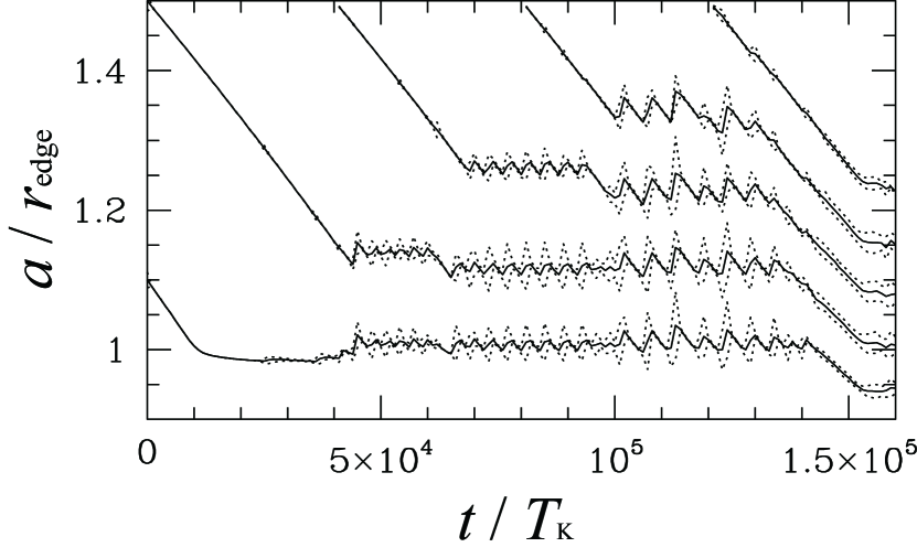
Figure 6: Orbital evolution of multiple ($n>2$) Earth-mass planets in the fiducial case ($\Delta r/r_{\rm edge}=0.01$ and $t_{e}/t_{a}=10^{-3}$). Solid lines are semimajor axes, and dotted lines are pericenters and apocenters.

To confirm Eq. (35), we performed a calculation with $n\geq 3$ in the fiducial case with $\Delta r/r_{\rm edge}=0.01$ and $t_{e}/t_{a}=10^{-3}$. In this case, Eq. (35) is reduced to $n<5$. Individual planet masses are one Earth mass. The orbital evolution is shown in Fig. 6. After the first planet is trapped at the edge, subsequent migrating planets are trapped one after another. After $10^{5}T_{\rm K}$, four planets are trapped by the edge torque. But, when the fifth planet is trapped, the edge torque no longer halts the planets outside the edge and the they migrate inward as a whole. The innermost planet is pushed into the cavity. After $1.5\times 10^{5}T_{\rm K}$, four planets are outside the edge and the edge torque exerted on the second planet supports the outer two planets. The result of N-body simulation is in a good agreement with the analytical estimate, $n<5$.

With the value of $t_{e}/t_{a}\sim 10^{-5}$ that Ogihara & Ida (2009) used in their slow migration case, Eq. (35) shows that $n<500$. This is consistent with their result in which they found that all the (20–30) migrating planetary embryos are trapped and remain outside the disk edge.

3.4 Supersonic Correction

The Tanaka & Ward’s formulas assume subsonic flow. However, for the eccentricity trap to be efficient, eccentricity $e$ must be pumped up by resonance to be $ea\gtrsim H$, that is, $ev_{\rm K}\gtrsim c_{s}$. In this case, the relative motion between gas and planets can be supersonic. According to Ostriker (1999), we also carried out runs with the $e$-damping forces (Eqs. [2]–[4]) multiplied by a supersonic correction factor, $1/(1+(ev_{\rm K}/c_{s})^{3})$. Then, the effective damping timescale $t_{e,\rm{eff}}$ is defined as

$$t_{e,\rm{eff}}\equiv t_{e}\times\left[1+\left(\frac{ev_{\rm K}}{c_{s}}\right)^{3}\right],$$ (36)

where $t_{e}$ is the Tanaka & Ward’s damping timescale (Eq. [5]). This supersonic correction is consistent with that obtained by Papaloizou & Larwood (2000).

Because $t_{e,\rm{eff}}$ is larger than $t_{e}$ for supersonic cases, this correction is negative for the eccentricity trap. However, Papaloizou & Larwood (2000) showed that supersonic correction is also applied for the $a$-damping. The correction factor for the $a$-damping timescale is $(1+(ev_{\rm K}/c_{s})^{5})/(1-(ev_{\rm K}/c_{s})^{4})$, which is a stronger function of $ev_{\rm K}/c_{s}$ than that for the $e$-damping timescale and even changes sign to make the migration outward. With the corrections for both $a$ and $e$ damping, the eccentricity trap is rather strengthen in supersonic cases. Here, we include the supersonic correction only for the $e$-damping in N-body simulations, which significantly underestimates the efficiency of the eccentricity damping. Nevertheless, the eccentricity trap still occurs for likely values of $t_{e}/t_{a}$, although the region of the eccentricity trap on the $\Delta r/r_{\rm edge}-t_{e}/t_{a}$ plane is more restricted.

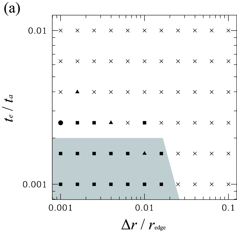
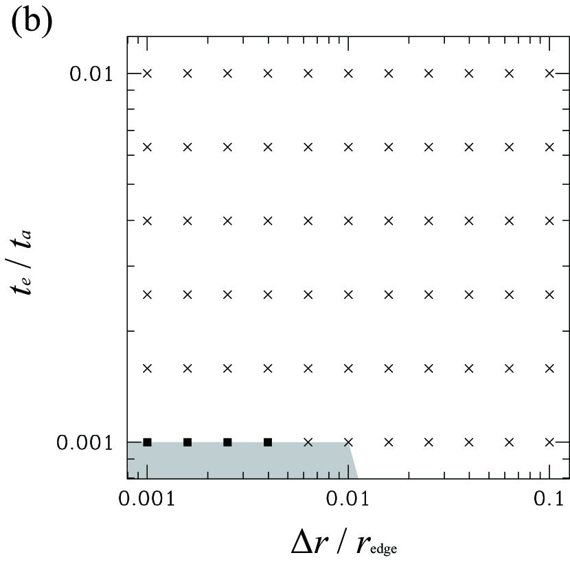
Figure 7: Same as Fig. 3, but with supersonic correction factor. (a) Case with $c_{s}/v_{\rm K}\simeq 0.03$. (b) Case with $c_{s}/v_{\rm K}\simeq 0.02$. The shaded region is the analytically predicted trapping regions. Note that $t_{e}$ is not the effective damping timescale.

Figure 7 summarizes the results with the supersonic correction on the $\Delta r/r_{\rm edge}-t_{e}/t_{a}$ plane. (Note that $t_{e}$ which is used in the vertical axis is not the effective damping timescale but that for subsonic cases described in Eq. [5].) Figure 7a and 7b are the cases with $c_{s}/v_{\rm K}\simeq$ 0.03 and 0.02, respectively. While the eccentricity trap regions are more restricted, in particular, in Figure 7b, they still exist. The shaded regions in Fig. 7 represent the (conservative) analytical condition (Eq. [18]) with the effective damping timescale, which are consistent with the numerical results.

4 CONCLUSION

We propose a mechanism that we call an “eccentricity trap” of migrating planets and investigated the details of the trapping condition both analytically and numerically. This halting mechanism is so strong that many resonantly-interacting planets are trapped by the edge torque that is exerted only on an innermost planet at the inner disk edge, as long as the edge is sharp enough ($\Delta r<r_{\rm edge}$; $\Delta r$ is the edge width and $r_{\rm edge}$ is the edge radius.) and the eccentricity damping timescale due to planet-disk interaction ($t_{e}$) is short enough compared with semimajor axis damping timescale ($t_{a}$). The explicit trapping condition is given by

$$\frac{t_{e}}{t_{a}}<\frac{fe}{2\pi},$$ (37)

where

$$f\simeq\left\{\begin{array}[]{ll}1&(\mbox{for }er_{\rm edge}>\Delta r)\\ {\displaystyle\sqrt{\frac{er_{\rm edge}}{\Delta r}}}&(\mbox{for }er_{\rm edge}<\Delta r).\end{array}\right.$$ (38)

The evaluation for the eccentricity of the innermost body, $e$, is given by Eqs. (23) and (24).

As discussed in section 3.1, near the inner disk edge ($\lesssim 0.1$AU), the sound velocity scaled by Kepler velocity is so small that disk scale height may be sharp ($\Delta r/r_{\rm edge}\sim 10^{-2}$) and $t_{e}/t_{a}$ is as small as $10^{-4}$–$10^{-3}$ even if we assume the formulas for the $a$ and $e$ damping by Tanaka et al. (2002) and Tanaka & Ward (2004). Therefore, the eccentricity trap condition is safely satisfied in protoplanetary disks, if they have a cavity. When the motion of the planet is supersonic ($ev_{\rm K}>c_{s}$), damping formulas are modulated. Then, the eccentricity trap is strengthen.

We also derived a formula for the maximum number of trapped planets outside the edge. It explains the result of Ogihara & Ida (2009), where 20–30 planets are lined up outside the disk edge in the case of slow migration. This is an essential point of Ogihara & Ida (2009)’s model for formation non-resonant, multiple, close-in super-Earths at $\sim 0.1$AU. The innermost planet is pinned to the disk inner edge (at $\sim 0.05$AU) and the convoy of the resonantly trapped planets extends well beyond 0.1AU. After gas dispersal, they undergo orbital crossing and are kicked out of the resonances, leading to many giant impacts to increase the planetary mass by more than a factor of 10. As a result, a few super-Earths are accreted at $\sim 0.05$–0.3AU. Since their masses exceed several Earth masses after disk dissipation, they avoid the gas accretion necessary to become gas giant planets, as we show in a sequential planet formation model in a separate paper (Ida & Lin, 2010). The resultant non-resonant, multiple super-Earths systems at $\sim 0.1$AU are consistent with observed data. The discovered close-in super-Earth systems (GJ 581 and HD 40307) do not have any commensurate relationships, and orbits of outer planets extend beyond 0.1 AU, which can be formed reasonably by the above model if clear cavities existed in their progenitor disks.

This trapping mechanism also provides deep insights into satellite formation around giant planets. Based on the slow inflow disk model (e.g., Canup & Ward 2002, 2006), $c_{s}/v_{\rm K}\sim 0.06$ and we found through a preliminary N-body simulation that $e\sim 0.1$ for resonantly trapped satellites. Equation (33) suggests that a few Galilean satellites are trapped outside the disk edge. If more satellites are trapped to violate the trapping condition, the innermost one is pushed into the inner cavity. Since the disk edge would coincide with corotation radius with the host object’s spin, the innermost satellite in the cavity loses its orbital angular momentum by tidal torque from Jupiter to collide with it. As a result, resonant trapping of a few satellites may be always maintained. Because the number of the trapped satellites are relatively small, the satellites may remain stable after gas dissipation. An outermost satellite, Callisto, which is not in a resonance, may accrete in the outer residual disk. More detailed study of satellite formation is discussed in Sasaki et al. (2010) and a forthcoming paper (Ogihara et al. in preparation).

The validity of applying the $e$-damping formulas by Tanaka & Ward (2004) for nonuniform region near the disk edge should be tested by hydrodynamical simulations. At the same time, reverse torque for type I migration (Masset et al., 2006), which is not considered here, should also be considered as well. Although we simply assumed the disk edge width is similar to the disk scale height, disk edge structure may be created by stellar magnetic field. Thus MHD simulations are also needed to determine the disk edge structure. Furthermore, the conditions necessary to maintain a cavity should also be investigated by MHD simulation.

ACKNOWLEDGMENT

We thank fruitful and stimulating discussions with Steve Lubow, Bill Ward, Doug Lin, John Papaloizou, Aurélien Crida, Clement Baruteau, and Sijme-Jan Paardekooper during our participation in “Dynamics of Discs and Planets” workshop at the Newton Institute at Cambridge University, where some of this work was done. We also thank the anonymous referee for helpful comments, and thank Hidekazu Tanaka, Taku Takeuchi and Takayuki Muto for valuable suggestions. This work was supported by Grant-in-Aid for JSPS Fellows (2008528).

References

- Artymowicz (1993) Artymowicz, P. 1993, ApJ, 419, 166
- Binney & Tremaine (1987) Binney, J., & Tremaine, S. 1987, Nature, 326, 219
- Bouchy et al. (2009) Bouchy, F., Mayor, M., Lovis, C., Udry, S., Benz, W., Bertaux, J. -L., Delfosse, X., Mordasini, C., Pepe, F., Queloz, D., & Segransan, D. 2009, A&A, 496, 527
- Canup & Ward (2002) Canup, R. M., & Ward, W. R. 2002, ApJ, 124, 3404
- Canup & Ward (2006) Canup, R. M., & Ward, W. R. 2006, Nature, 441, 834