AMENDART in Markovian circuit QED

Abstract

We study the cavity field’s and atomic asymptotic mean excitation numbers due to anti-rotating term (AMENDART) in the circuit Quantum Electrodynamics (circuit QED) system, composed of a two-level atom and a single cavity field mode, subject to Markovian damping and dephasing mechanisms. We show that the AMENDART are above the thermal values, and their behavior is analyzed analytically and numerically for typical parameters in circuit QED implementations described by the Rabi Hamiltonian. We point out that “parasitic elements”  such as other cavity modes or eventual off-resonant atoms, also contribute substantially to AMENDART.

I Introduction

Cavity Quantum Electrodynamics (cavity QED) is one of the most active areas of research in quantum optics and quantum information nowadays. It deals with the light-matter interaction for electromagnetic (EM) fields with a few photons and a small number of real or artificial atoms confined in optical and microwave resonators. It can be implemented in a variety of architectures, such as atomic ensembles, Rydberg atoms, quantum dots, superconducting circuits, Bose-Einstein condensates, polar molecules, trapped ions, etc Walmsley ; Walmsley1 ; Walmsley2 ; Walmsley3 ; Walmsley4 ; Harro . Here we focus on the cavity QED realizations in superconducting circuits, the area known as circuit QED Blais ; refe , where the one-photon–one-atom interaction is currently realized with different types of artificial atoms, and interaction between different atoms, placed deterministically inside the cavity, is realized by means of the cavity field acting as the quantum bus. Some advantages of using superconducting circuits are the possibility of engineering the properties of the artificial atoms, such as the energy levels configuration and the atom-field coupling, rapid tuning of the cavity’s and atom’s frequencies and the freedom in fabricating several artificial atoms at specific locations within the cavity. Besides studying fundamental problems in quantum mechanics, such as entanglement, dissipation, decoherence and the measurement problem, circuit QED is also an important tool for testing basic quantum algorithms dicarlo , engineering nonclassical states of light and matter Walmsley ; Walmsley4 ; Har2 , achieving the strong and ultra-strong light-matter coupling Hows ; Hows1 , implementing rapid time-dependent phenomena Libe ; Libe1 ; Liberato ; Lukin ; Lukin1 ; v7 ; v9 ; duty and novel technologies for quantum information processing Walmsley4 ; QIP , etc.

The simplest Hamiltonian, deduced from first principles, that describes the interaction between a two-level atom and a single mode of the quantized electromagnetic field in a cavity is the Rabi Hamiltonian (RH) Rabi . It reads $(\hbar=1)$

$$H_{R}=n+\Omega E+g\,p\sigma_{y},$$ (1)

where we set the cavity frequency to $\nu=1$, the atomic transition frequency is $\Omega$ and $g$ is the atom-field coupling constant. The cavity field quadrature operators are $x=(a^{\dagger}+a)/\sqrt{2}\$and $p=i(a^{\dagger}-a)/\sqrt{2}$, $a$ and $a^{\dagger}$ are the bosonic annihilation and creation operators, satisfying the commutation relation $[a,a^{\dagger}]=1$, and $n=a^{\dagger}a$ is the photon number operator. The atomic operators are $E=\left|e\right\rangle\left\langle e\right|$, $\sigma_{x}=\sigma_{-}+\sigma_{+}$, $\sigma_{y}=i(\sigma_{-}-\sigma_{+})$ and$~{}\sigma_{z}=E-|g\rangle\langle g|$, where $\sigma_{+}=\left|e\right\rangle\left\langle g\right|$ and $\sigma_{-}=\sigma_{+}^{\dagger}$, $\left|g\right\rangle$ and $\left|e\right\rangle$ denoting the ground and excited atomic states, respectively. The exact diagonalization of RH has not been achieved yet, so to obtain analytical results one usually performs the Rotating Wave Approximation (RWA) by neglecting the anti-rotating term (ART) $(a\sigma_{-}+a^{\dagger}\sigma_{+})$, responsible for simultaneous creation/annihilation of one photon and one atomic excitation Scully ; Schleich . In this case one gets the celebrated Jaynes-Cummings Hamiltonian (JCH) JC ; JC1 , which has a simple analytical solution Scully ; Schleich ; Harro that led to prediction of several pure quantum effects, many of them already verified experimentally Harro ; Walmsley ; Walmsley1 ; Walmsley2 ; Har1 ; Har2 ; Har3 ; refe .

The RH or JCH alone do not describe the current situation in circuit QED because of dissipation and decoherence arising from the system interaction with cavity’s and atomic environments. So instead of the Schrödinger equation one has to use the quantum master equation for the density operator $\rho$, whose general form is Scully ; Schleich ; Breuer ; Carm

$$\frac{d}{dt}{\rho}+i[H,\rho]=\mathcal{L}\rho,$$ (2)

where $H$ is some effective Hamiltonian and the superoperator $\mathcal{L}$ is the Liouvillian that accounts for the influence of the environment. In most situations the Liouvillian consists of three parts, $\mathcal{L}=\mathcal{L}_{\kappa}+\mathcal{L}_{\lambda}+\mathcal{L}_{\gamma}$, where the superoperator $\mathcal{L}_{\kappa}$ ($\mathcal{L}_{\lambda}$) describes the cavity (atom) damping by the thermal reservoir with the mean photon number $\bar{n}$, and $\kappa$ ($\lambda$) is the cavity (atom) relaxation rate that can be determined experimentally Walmsley ; Harro ; refe ; refe1 ; Har1 ; Har2 ; Har3 . Another common source of decoherence in superconducting circuits is the pure atomic dephasing represented by $\mathcal{L}_{\gamma}$, that arises due to low-frequency $1/f$ noise Clarke , and $\gamma$ denotes the pure dephasing rate Carm ; Makhlin . The preferred theoretical pick to describe the majority of experiments, owing to its simplicity and wide applicability range, is the “standard master equation” (SME) Harro ; Har1 ; Blais ; refe ; refe1

$$\mathcal{L}_{\kappa} = \kappa(\bar{n}+1)\mathcal{D}[a]+\kappa\bar{n}\mathcal{D}[a^{\dagger}]$$ (3)

$$\mathcal{L}_{\lambda} = \lambda(\bar{n}+1)\mathcal{D}[\sigma_{-}]+\lambda\bar{n}\mathcal{D}[\sigma_{+}]$$ (4)

$$\,\mathcal{L}_{\gamma} = \frac{\gamma}{2}\mathcal{D}[\sigma_{z}],$$ (5)

that can be deduced microscopically by making the Born-Markovian approximation on the system-reservoir interaction Carm , where the so called Lindblad superoperator

$$\mathcal{D}[\Phi]\rho\equiv\frac{1}{2}\left(2\Phi\rho\Phi^{\dagger}-\Phi^{\dagger}\Phi\rho-\rho\Phi^{\dagger}\Phi\right)$$ (6)

preserves the hermiticity, normalization and positivity of $\rho$ Breuer .

Within the quantum trajectories approach a Markovian reservoir represented by a Lindblad kernel can be viewed as a “detector” performing continuous measurements on the system Breuer ; prel ; engi . Considering, for instance, $\mathcal{L=}\chi\mathcal{D}[\Phi]$ and rewriting (2) as $d\rho/dt-L\rho=R\rho$, where $R\rho\equiv\chi\Phi\rho\Phi^{\dagger}$ and $L\rho\equiv-i[H,\rho]-\{\Phi^{\dagger}\Phi,\rho\}\chi/2$, one may check that the formal solution for $\rho(t)$ is Carm

$$\rho(t) = \sum_{m=0}^{\infty}\int_{0}^{t}dt_{m}\int_{0}^{t_{m}}dt_{m-1}\cdots\int_{0}^{t_{2}}dt_{1}\tilde{\rho}_{m}$$ (7)

$$\tilde{\rho}_{m} \equiv e^{L(t-t_{m})}Re^{L(t_{m}-t_{m-1})}\cdots Re^{Lt_{1}}\rho\left(0\right).$$ (8)

This procedure decomposes the quantum dynamics contained in the master equation into an infinity of quantum trajectories, where each occurrence of $R$ corresponds to an instantaneous quantum jump of the system’s state engi , and the exponentials $\exp[L_{0}(t_{k}-t_{k-1})]$ describe the non-unitary system evolution between the quantum jumps. Thus $\tilde{\rho}_{m}$ can be interpreted as the evolved (non-normalized) density operator conditioned to quantum jumps at times $t_{1},t_{2}\ldots t_{m}$, and its trace gives the probability of this particular sequence. Such an interpretation describes the Markovian dissipation as continuous measurement of the system by the reservoir prel , where the quantum jumps describe the “clicks” of the “detector” engi , and the exponential superoperators describe the system evolution without “clicks” but still under continuous monitoring Breuer ; Carm .

The JCH shows good agreement with experiment and with numerical calculations in the majority of problems of practical interest Har3 . However, in some occasions the ART becomes important, so many studies investigated the range of validity of RWA and new physics beyond RWA (see references in CAMOP ). In particular, in Werlang1 was shown that the combined action of the anti-rotating term and Markovian dissipation leads to incoherent photon creation from vacuum, so the asymptotic mean photon number is slightly above the thermal value. A detailed analysis of this phenomenon was performed in CAMOP , in Werlang3 the cavity emission rate due to ART was calculated, and the relation of ART to the entropy operator was described in Kurcz2 . Moreover, in the study 2atoms the errors in the zero-excitation state preparation due to ARTs in two-atom Markovian cavity QED system were estimated, while the creation of transient entanglement between two atoms due to ARTs was reported in Jing .

Here we study analytically and numerically the cavity field’s and atomic asymptotic mean excitation numbers due to anti-rotating term (AMENDART) for the current parameters in circuit QED, taking into account common “parasitic” elements, such as other cavity modes and off-resonant two-level atoms, showing that in many cases these elements contribute significantly to the generation of atomic and cavity field’s excitations due to ART.

II Analytical and numerical results

In this section we analyze analytically and numerically the asymptotic mean numbers of photons and atomic excitations, $\left\langle n\right\rangle$ and $\left\langle E\right\rangle$, respectively, in the circuit QED setup described by the master equation (2) with $H=H_{R}$ and dissipative kernels (3)-(5). Since RH cannot be integrated exactly, to obtain approximate analytical results we perform the $k$-photons approximation (denoted below by the subindex $k$) by assuming that at most $k$ photons are present in the cavity. The asymptotic values are evaluated by equaling to zero the left-hand-side of the resulting Heisenberg equations of motion. Under the $1$-photon approximation, valid for $\left\langle n_{1}\right\rangle\ll 1$, for zero-temperature damping reservoirs ($\bar{n}=0$) we get simple formulae for the AMENDART CAMOP

$$\left\langle n_{1}\right\rangle = \frac{G}{T}\left(2G+\lambda s\right)$$ (9)

$$\langle E_{1}\rangle = \frac{G}{T}\left(2G+\kappa s\right),$$ (10)

where $G=g^{2}\Gamma$, $\Gamma=\gamma+(\kappa+\lambda)/2$, $s=\Delta^{2}+\Gamma^{2}$, $T=2G[\alpha(\kappa+\lambda)+2G]+\lambda\kappa\beta$, $\alpha=s+2\Omega$ and $\beta=\alpha^{2}-4\Omega^{2}$. Here $\Delta\equiv\Omega-1$ is the atom-cavity detuning and $\left\langle\cdots\right\rangle$ denotes the asymptotic value. One may also obtain another useful expression for estimating the correlation between the atom and the field

$$\left\langle(n\sigma_{z})_{1}\right\rangle=\frac{\lambda}{\lambda+\kappa}\left(\left\langle E_{1}\right\rangle-\left\langle n_{1}\right\rangle\right).$$ (11)

For higher orders approximations the formulae are not so compact, so below we shall present only the numerical results for the $2$-photons approximation.

In many practical situations the circuit QED system contains other elements, apart from the selected cavity mode and the artificial atom. In particular, the atom always interacts with other cavity modes, usually neglected due to their strong detuning from the atomic transition frequency and because initially they are not populated by photons. In ordinary cavities realized as coplanar waveguide resonators the modes are regularly spaced in frequency, and if the atom is fabricated at one end of the resonator, then all the cavity modes have a voltage antinode at the atom’s position Blais . To check whether other cavity modes are relevant for the phenomenon of photon generation due to the ART, we suppose that, besides the selected cavity mode (the “true mode”), the atom also interacts with another cavity mode with frequency $\tilde{\nu}$ and the corresponding coupling constant $\sqrt{\tilde{\nu}}g$ – a “parasitic mode”, whose variables are denoted with tilde. In this case the total Hamiltonian becomes Scully ; Schleich

$$H=H_{C}\equiv H_{R}+\tilde{\nu}\tilde{n}+\sqrt{\tilde{\nu}}g\,\tilde{p}\sigma_{y},$$ (12)

and assuming that the cavity quality factor is the same for the two modes, the corresponding modification in the Liouvillian is

$$\mathcal{L}_{C}=\mathcal{L}+\tilde{\nu}\kappa\mathcal{D}[\tilde{a}].$$ (13)

Based on common experimental conditions, we assume that initially the parasitic mode is in the vacuum state, and consider two plausible scenarios. a) The true mode ($\nu=1$) is the fundamental mode of the half-wave resonator, and the parasitic mode corresponds to the first harmonic full wavelength resonance, $\tilde{\nu}=2$. b) The opposite scenario: the true mode ($\nu=1$) corresponds to the first harmonic full wavelength resonance, and the parasitic mode is the half-wave fundamental mode, $\tilde{\nu}=1/2$. Below we distinguish between these two cases by indicating the value of $\tilde{\nu}$.

Furthermore, in some circuit QED setups two almost identical artificial 2-level atoms are fabricated within the same cavity to perform two-atoms quantum gates, where the cavity mode plays the role of a quantum bus. When one is interested in performing only one-atom quantum gates, the second atom is effectively “turned off” by tuning its transition frequency $\tilde{\Omega}$ far apart from the cavity mode’s and the other atom’s frequencies. So we study the scenario where the “connected” atom is the “true atom” and the “disconnected” one acts as the “parasitic atom” (its variables are denoted with tilde), so the total Hamiltonian and the Liouvillian become 2atoms

$$H=H_{A}\equiv H_{R}+\tilde{\Omega}\tilde{E}+g\,p\tilde{\sigma}_{y}$$ (14)

$$\mathcal{L}_{A}=\mathcal{L}+\lambda\mathcal{D}[\tilde{\sigma}_{-}]+\frac{\gamma}{2}\mathcal{D}[\tilde{\sigma}_{z}],$$ (15)

where we assumed that the coupling constants and the dissipative rates are the same for the both atoms. We shall consider two scenarios: c) the parasitic atom transition frequency is significantly smaller than the cavity mode frequency, $\tilde{\Omega}=0.2$, or d) is significantly larger, $\tilde{\Omega}=1.8$.

Below we study numerically the AMENDART of the true cavity mode, $\left\langle n\right\rangle$, and the true atom, $\left\langle E\right\rangle$, as function of the system parameters under the $1$- and $2$- photon approximations. We verified that in the weak coupling limit, $g\ll 1$, these quantities grow up approximately quadratically in $g$, so in the figures 1 – 4 we set $g=5\times 10^{-2}$, a value that can be achieved in some circuit QED systems and is within the weak coupling limit. Moreover, as we are interested in the lower bounds for the mean excitation numbers, we set the reservoir temperatures to $0\,\mathrm{K}$, $\bar{n}=0$. This simplification does not restrict the scope of our analysis, since we verified that for small but finite temperatures ($\bar{n}\ll 1$) the cavity’s and atomic excitations due to finite temperature are approximately added to the AMENDART (data not shown).

In the figure 1 we show how $\left\langle n\right\rangle$ and $\left\langle E\right\rangle$ depend on the true atom transition frequency $\Omega$ in the presence of parasitic elements for parameters indicated in the caption, that can be achieved in the near future experiments. The dashed lines correspond to the $1$-photon approximation and the solid lines – to the $2$-photons approximation. We see that for the chosen parameters the $1$-photon approximation is quite accurate, and out of resonance the AMENDART decrease as function of $\Omega$. In the figure 2 we perform a similar analysis as function of the pure dephasing rate, from which we see that the AMENDART grow up as function of $\gamma$, and the $1$-photon approximation loses its accuracy as $\left\langle n\right\rangle$ (or $\gamma$) increases. Remarkably, in these cases the parasitic elements cannot be neglected, since they contribute substantially to the AMENDART. Therefore, if one wants to know precisely the values of AMENDART in circuit QED systems, one has to take into account the parasitic elements, even when they are far detuned and initiated in their respective ground states.

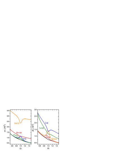
Figure 1: AMENDART as function of atomic transition frequency for parameters $\kappa=\lambda=10^{-6}$ and $\gamma=\lambda/4$ in the presence of parasitic elements, whose parameters are indicated in the plots. Dashed lines correspond to the $1$-photon approximation, and the solid ones – to the $2$-photons approximation.

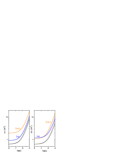
Figure 2: AMENDART as function of $\gamma$ for parameters $\kappa=\lambda=10^{-6}$, $\Omega=1$ in the presence of parasitic elements, whose parameters are indicated in the plots. The solid lines correspond to the $2$-photons approximation, and the dashed ones – to the $1$-photon approximation.

Despite a finite asymptotic photon population in the true cavity mode, it cannot be associated to an effective temperature reservoir Klimov , since the resulting distribution is significantly different from the thermal one. This is illustrated in the figure 3a, where we show the probability $P_{n}$ of having $n$ photons in the cavity, obtained under the $2$-photons approximation in the presence of the parasitic atom for parameters indicated in the caption (filled black bars). For comparison we also show the thermal distribution with the same mean photon number (red bars with sparse pattern), whereby one can see that the two distributions are quite different. Besides, there is a correlation between the “true field” and the “true atom” in the asymptotic state, as quantified by the quantum mutual information, that measures the total amount of correlation in a bipartite quantum state Nielsen

$$I_{af}=S\left(\rho_{a}\right)+S\left(\rho_{f}\right)-S\left(\rho_{af}\right).$$ (16)

Here $S\left(\rho_{k}\right)=-\mathrm{Tr}[\rho_{k}\log_{2}(\rho_{k})]$ is the von Neumann entropy of the $k$th subsystem whose dynamics is described by the reduced asymptotic density matrix $\rho_{k}$ with $k=\{atom,field,atom-field\}$. $I_{af}$ is shown in the figure 3b as function of $\Omega$ in the absence of the parasitic elements (black lines), and when the “parasitic atom” (orange lines) or “parasitic mode” (blue lines) are present for parameters $\kappa=\lambda=10^{-6}$ and $\gamma=\lambda/4$. The dashed (solid) lines correspond to the $1$ ($2$)-photon approximation, and the results for the $1$-photon approximation in the absence of the parasitic elements can be obtained analytically with the aid of equations (9)-(11). One can see that asymptotically the atom-field system is correlated, $I_{af}\neq 0$, and the mutual information decreases in the presence of the parasitic elements, since in this case they acquire some information about the system of interest.

One can also notice from the right plot of figure 3a that when the true atom is out of resonance, $\left\langle n\right\rangle$ is larger for smaller $\kappa$. This is better depicted in the figure 4, where we show the total asymptotic mean excitation number under the $2$-photons approximation, $\left\langle n_{2}\right\rangle+\left\langle E_{2}\right\rangle$, as function of damping rates under the resonance (sparse white curve) and out-of-resonance (filled colored curve) conditions in the presence of the parasitic atom, with the system parameters indicated in the caption. One can see that at the resonance $\left\langle n_{2}\right\rangle+\left\langle E_{2}\right\rangle$ does not depend strongly on the damping rates, contrary to out-of-resonance case, where it is smaller when $\kappa$ and $\lambda$ are approximately equal.

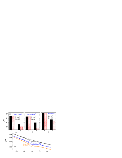
Figure 3: a) Photon number distribution for parameters $\tilde{\Omega}=0.2$, $\lambda=10^{-6}$, $\gamma=\lambda/4$ and $\kappa$ and $\Omega$ as indicated in the plots. Filled black bars describe the photon distribution due to AMENDART, and the red bars with sparse pattern correspond to the thermal distribution with the same $\left\langle n\right\rangle$. b) Quantum mutual information $I_{af}$ for the asymptotic state with and without the parasitic elements.

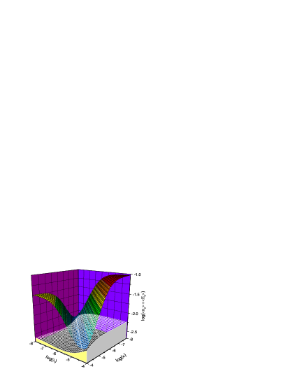
Figure 4: Logarithm of the total mean excitation number $\log(\left\langle n_{2}\right\rangle+\left\langle E_{2}\right\rangle)$ as function of $\log(\kappa)$ and $\log(\lambda)$ in the presence of the parasitic atom, for parameters $\gamma=\lambda/4$ and $\tilde{\Omega}=0.2$. The colored curve corresponds to out-of-resonance case, $\Omega=0.7$, and the white one to the resonance, $\Omega=1.$

III Discussion and generalizations

The phenomenon of excitations generation above the thermal values occurs due to the combined action of the ART in the RH and the Markovian approximation for the reservoirs CAMOP . The ART describes continuous spontaneous creation from vacuum and annihilation of virtual atomic and photonic excitations Scully ; Schleich . Under the Markovian approximation, the reservoir correlation time is very short compared to the time scale for a significant change in the system Carm , i.e. the time needed to annihilate excitations. Therefore, once the excitations are spontaneously created, a fraction of them decays to the reservoir due to atomic and/or cavity damping before they can be annihilated, so the system coherence is destroyed and the initial zero-excitation state cannot be restored. From the point of view of quantum trajectories Breuer ; Carm ; prel , the continuous monitoring of the system by the Markovian environment promotes the virtual excitation into real ones due to the continuous change of system’s state, while a fraction of the excitations is destroyed due to destructive measurements, thereby asymptotically nonzero photon and atomic populations are built in the system. The pure atomic dephasing increases the number of created excitations Werlang1 because the dephasing reservoir performs nondestructive measurement of the atomic state Carm , so the virtual excitations are promoted into real ones nondestructively. Besides, the Markovian pure atomic dephasing can be attributed to random changes of the atomic transition frequency refe ; Makhlin ; Werlang1 , which promote the virtual excitations into real ones due to the modification of the system ground state, analogously to the dynamical Casimir effect Liberato ; Book ; Lukin ; Lukin1 . It is worth noting that, by definition, the pure dephasing reservoir always has a finite temperature Carm , whereby it can perform nondestructive measurements of the atomic state, so the substantial amplification of system excitations due to pure Markovian dephasing is not so puzzling.

The phenomenon of nonzero asymptotic photon population also occurs for a single dissipative cavity if one takes into account the anti-rotating cavity-reservoir interaction. Suppose we isolate a single constituent of the reservoir (e.g. 2-level atom, harmonic oscillator, etc) and treat it as an ancilla; then, one performs the standard Born-Markovian master equation treatment over the remaining reservoir constituents. Thereby we obtain a Markovian master equation for the cavity-ancilla system, including the anti-rotating interaction. By performing the asymptotic analysis of the previous section and tracing over the ancilla variables at the end, one would end up with a nonzero photon population due to the virtual cavity-ancilla excitations being promoted into real ones by the Markovian reservoir. Another way of arriving at this conclusion is to use the simplified phenomenological approach. The most general master equation for a single cavity field mode Dekker ; Me , preserving the normalization and hermiticity of the statistical operator $\rho$ and containing only bilinear forms of operators $x$ and $p$ is given by the equation (2) with the effective Hamiltonian

$$H=H_{0}+\frac{\mu}{4}\left\{x,p\right\},$$ (17)

where $H_{0}=n$ is the cavity Hamiltonian (recalling that the cavity frequency is set to $\nu=1$), and the damping superoperator is $\mathcal{L}=\mathcal{L}_{\kappa}^{\prime}$

$$\mathcal{L}_{\kappa}^{\prime}\rho = \frac{i\kappa}{4}\left(\left[p,\left\{x,\rho\right\}\right]-\left[x,\left\{p,\rho\right\}\right]\right)-D_{p}\left[x,\left[x,\rho\right]\right]$$ (18)

$$- D_{x}\left[p,\left[p,\rho\right]\right]+D_{z}\left(\left[x,\left[p,\rho\right]\right]+\left[p,\left[x,\rho\right]\right]\right),$$

with $\mu$, $\kappa$, $D_{x}$, $D_{p}$ and $D_{z}$ being arbitrary time-independent coefficients under the Markovian approximation. The condition

$$D_{p}D_{x}-D_{z}^{2}\geq(\kappa/4)^{2}$$ (19)

guarantees that the positivity of the statistical operator is preserved for all times and for any physically admissible initial state. This is the necessary and sufficient condition (together with conditions $D_{x}\geq 0$ and $D_{p}\geq 0$) of reducibility of the superoperator (18) to the Lindblad form DOM85 . The standard master equation (3) corresponds to the choice $D_{p}=D_{x}=\kappa\left(1+2\bar{n}\right)/4$ and $D_{z}=\mu=0$, which satisfies the inequality (19).

One can verify CAMOP that asymptotically the vacuum state (with mean values $\langle x^{2}\rangle=\langle p^{2}\rangle=1/2$, $\langle\left\{x,p\right\}\rangle=0$) is achieved for the coefficients

$$D_{p}^{\prime}=(\kappa+\mu)/4,\quad D_{x}^{\prime}=(\kappa-\mu)/4,\quad D_{z}^{\prime}=0.$$ (20)

Using the inequality (19) one obtains $\kappa^{2}-\mu^{2}\geq\kappa^{2}$, whose solution is $\mu=0$. Therefore the vacuum state can be achieved only for the coefficients $D_{x}^{\prime}=D_{p}^{\prime}=\kappa/4$ and $\mu=D_{z}^{\prime}=0$, which correspond to the standard master equation (3) at zero temperature. However, the SME is deduced microscopically by making the RWA on the cavity-reservoir interaction Carm ; Scully ; Schleich , i.e. by neglecting the anti-rotating terms responsible for simultaneous creation of one virtual photon and a virtual reservoir excitation. Therefore, if the anti-rotating cavity-reservoir interactions are taken into account, under the Markovian approximation the asymptotic mean photon number in the dissipative cavity is larger than zero. Finally, if one uses a single dissipative kernel (18) together with the Hamiltonian (17) to describe the circuit QED system, with $H_{0}=H_{R}$, under the $1$-photon approximation one gets (for $g\neq 0$)

$$\left\langle n_{1}\right\rangle = \frac{1}{2}\left(1-\frac{1}{2}\frac{\kappa}{D_{xp}+2g^{2}D_{x}\phi}\right)>0$$ (21)

$$\langle E_{1}\rangle = \frac{1}{2}\left(1-\frac{1}{2}\frac{\kappa\Omega\phi\nu_{+}D_{xp}/D_{p}}{D_{xp}+2g^{2}D_{x}\phi}\right)>0,$$ (22)

where $D_{xp}=D_{x}+D_{p}$, $\nu_{\pm}=\left(1\pm 2D_{z}\right)$ and $\phi=\left[\Omega^{2}+4D_{x}^{2}+\nu_{+}\nu_{-}D_{x}/D_{p}\right]^{-1}$. This demonstrates that regardless of the exact form of the master equation and the amount of dissipative channels, under the Markovian approximation the asymptotic mean photon and the atomic excitation numbers are always greater than zero, so the vacuum state is never achieved exactly.

IV Summary

In summary, we studied the behavior of the cavity field’s and atomic asymptotic mean excitation numbers due to anti-rotating term (AMENDART) for typical parameters of the Markovian circuit QED system, showing that “parasitic elements” (such as other cavity modes and off-resonant atoms) contribute to these quantities, which are typically of the order of $10^{-3}$ when the atom-field coupling constant is within a few percents of the cavity resonant frequency. This result implies that whenever one uses a Markovian master equation to describe the circuit QED system, there is a small intrinsic uncertainty in the mean photon number and the atomic excitation probability that originates from the anti-rotating term in the light-matter interaction Hamiltonian.