Theory of the quasiparticle excitation in high T_c cuprates: quasiparticle charge and nodal-antinodal dichotomy

Abstract

A variational theory is proposed for the quasiparticle excitation in high T_c cuprates. The theory goes beyond the usual Gutzwiller projected mean field state description by including the spin-charge recombination effect in the RVB background. The spin-charge recombination effect is found to qualitatively alter the behavior of the quasiparticle charge as a function of doping and cause considerable anisotropy in quasiparticle weight on the Fermi surface.

I I. Introduction

High temperature superconductors are doped Mott insulators. For such a strongly correlated electron system, it is of fundamental importance to know if and how does the Landau quasiparticle excitations emerge and what is peculiar about their properties in case of their existence. In recent decades, experiments, especially the angle resolved photoemission(ARPES) and the scanning tunneling microscopic spectrum(STM) measurements have elucidated in great details the evolution of the quasiparticle properties of the high-T_c cupartes as a function of doping and temperatureShen ; Ding ; Hanaguri ; Kanigel . However, a comprehensive understanding of these experimental observations is still in its infancy stage.

The existence of the quasiparticle excitation is now well established in the superconducting state of the cupratesShen . In the overdoped regime, the observations basically agrees with our expectations for a conventional Landau Fermi liquid, where a large Fermi surface enclosing a volume consistent with the Luttinger theorem for a system with $1-x$ electron per unit cell is observed. Well defined quasiparticle peaks are found all around the Fermi surface too. However, below optimal doping, parts of the Fermi surface around the antinodal region become less and less clear with decreasing doping. This phenomena, which is dubbed as nodal-antinodal dichotomy, is tangled with the issue of the existence of two gap scales and small hole pocket Fermi surfaceTacon ; Tanaka ; Taillefer . While in the half filing limit, in which the cuprates develops antiferromagnetic long range order, it is generally believed that quasiparticle excitation exists in the form of spin polaron and form small hole pocket Fermi surface. How is this small hole Fermi surface evolved into the large electron Fermi surface in the overdoped regime is long unresolved problem in the study of the high temperature superconductivity.

Another issue about the quasiparticle excitation in high Tc cuprates is their electrodynamic response kernel, or more loosely, the quasiparticle chargeLee . As a result of the Mott physics, the zero temperature superfluid density of the cuprates scales roughly linearly with the density of the doped holes $x$, rather than the result of $1-x$ when the strong correlation effect is neglected. Take it literally, this would imply that in the ground state each electron carry a charge of order $x$ rather than one. So naively one would expect that the quasiparticle excitation above the ground state should also carry a charge of order $x$. However, measurements of the temperature dependence of the superfluid density indicates that this is not the case. The almost doping independence of the slope of the superfluid density curve as a function of temperature indicates that the electrodynamic response kernel of the nodal quasiparticle is almost a constant in the underdoped regime.

The total mobile charge density of a doped Mott insulator is given by density of the doped holes. This requirement can be trivially satisfied by a small hole Fermi surface enclosing an area of $x$, on which each quasiparticle carries a charge of order one, as happens in the antiferromagnetic ordered state. However, according to the Landau Fermi liquid theory, a system with an electron density of $1-x$ per unit cell and no symmetry breaking should always form a large Fermi surface enclosing an area of $1-x$. So if we neglect the possible anisotropy of the quasiparticle charge on the Fermi surface, one would be naturally led to the conclusion that the quasiparticle on the Fermi surface should each carry a charge of order $x$. We are thus in a situation of dilemma. The system should either violate the Luttinger theorem by possessing a small Fermi surface of area $x$ in the absence of symmetry breaking, or, while having a large Fermi surface that respects the Luttinger theorem, have strong anisotropy on it. Both of these scenarios points to the nontrivial nature of the quasiparticle properties in the cuprates. It should be noted that suggestions have been made that in a system with topological order, the Luttinger theorem should be modified to accomodate the topological degeneracySenthil ; Paramekanti and a small Fermi surface in the absence of symmetry breaking is in principle possible. However, up to date there is no evidence in support of such a exotic order in the high T_c cuprates.

The key to the physics of a doped Mott insulator is the local constraint of no double occupancy between the electrons. The slave Boson mean field theory, in which such a local constraint is treated in an average manner, predicts a large Fermi surface consistent with the Luttinger theoremLee ; Rantner . The quasiparticle weight and quasiparticle charge is however isotropic on the Fermi surface and both show linear scaling with the hole density $x$. Attempts has been made to go beyond the mean field theory by including the fluctuation effect but the answer is still inconclusiveLee . The fluctuation around the mean field configuration, which takes the form of gauge fluctuations, is notoriously hard to be analyzed as there is no mass term to control their behavior.

The origin of the gauge degree of freedom in the slave Boson formalism is just the no double occupancy constraint between the electrons. To account for such a local constraint, Gutzwiller projected mean field state of the form $\mathrm{P}_{\mathrm{G}}\gamma^{\dagger}_{\mathrm{k},\sigma}|\mathrm{d-BCS}\rangle$ has been studied extensively to address the quasiparticle problemGros ; Anderson ; Randeria ; Gros1 ; Yunoki ; Nave ; Shih ; Sorella ; Li . However, it is found that the Gutzwiller projected state inherits to a large extent the properties of the mean field theory. For example, it also predicts a large Fermi surface on which the quasiparticle weight is uniform. Both the quasiparticle weight and the quasiparticle charge still vanish in the half filling limit, albeit with some powers different from the mean field theory predictions.

Despite these problems, both the slave Boson mean field theory and the Gutzwiller projection scheme do capture one key feature of the cuprates as a doped Mott insulator: the strong particle-hole asymmetry in the vicinity of the Fermi energy, which is hard to envisage in alternative scenarios where strong correlation effect is ignoredRantner ; Li ; Anderson . For this reason, we believe that the slave Boson mean field theory and the Gutzwiller projected state are good starting point for a more consistent theory.

An important consequence of the gauge fluctuation beyond the mean field description is the so called spin-charge recombination effectLee ; Wen . The gauge fluctuation, which couples equally to the spinon and the holon degree of freedom in the slave Boson formalism, will induce mutual backflow effect between the two parts. Such a backflow effect, which manifests itself as a kinematic effect of the local constraint, is beyond the reach of the Gutzwiller projection description and encourages the formation of spinon-holon bound state, whose motion is less affected by the gauge fluctuation.

To account for such a spin-charge recombination effect, a RPA theory has been proposed previouslyLee2 . The theory introduced a phenomenological attractive interaction between the spinon and the holon to induce spinon-holon bound state which is interpreted as the quasiparticle excitation of the system. Although the theory does have the potential to explain certain features of the experiments, it is not clear to what extent the predictions made by it are gauge invariant. The prediction power of the theory is also limited by its phenomenological nature and the sum rule for the electron spectral function is in general violated. Alternatively, a dopon-spinon formalism is introduced to account for the spin-charge recombination effect in which the bare hole is treated as an elementary degree of freedomRan . However, variational calculation based on this formalism can only be proceeded in the half filling limit with a small and finite number of doped holes.

In this paper, we extend the Gutzwiller projection description of the quasiparticle by including the backflow effect between the spinon and the holon at the wave function level. Our approach has the advantage that its predictions are gauge invariant and the electron spectral function calculated from it satisfy the relevant sum rule. We found the quasiparticle charge after the backflow effect correction approaches to a constant value in the half filling limit, rather than vanishes as predicted by the mean field theory and the Gutzwiller projection scheme. At the same time, the quasiparticle weight is found to show more and more strong anisotropy on the Fermi surface with decreasing doping and by fine tuning of the Hamiltonian parameters one can indeed reproduce the nodal-antinodal dichotomy phenomena in the cuprates.

This paper is organized as follows. In the next section, we review the variational description of the quasiparticle excitation in the Gutzwiller projection scheme and motivate our new variational wave function by reformulating the Gutzwiller projected wave function in terms of the slave Boson language in which the spin-charge recombination effect can be easily included. In section III, we introduce the numerical algorithm to do calculation on the wave function we have proposed. In section IV, we present our numerical results on both the doping dependence of the quasiparticle charge and the anisotropy of the quasiparticle weight on the Fermi surface. In section V, we present some discussion on the results. The appendix contains some details of the derivations in the text.

II II. Variational quasiparticle wave function

The model studied in this paper is the $t-J$ model,

$$\mathrm{H}=-\sum_{i,j,\sigma}t_{i,j}(\hat{c}^{\dagger}_{i,\sigma}\hat{c}_{j,\sigma}+h.c.)+J\sum_{\langle i,j\rangle}(\vec{S}_{i}\cdot\vec{S}_{j}-\frac{1}{4}n_{i}n_{j}),$$ (1)

in which $\hat{c}_{i,\sigma}$ is the electron operator satisfying the no double occupancy constraint $\sum_{\sigma}\hat{c}^{\dagger}_{i,\sigma}\hat{c}_{i,\sigma}\leq 1$, $t_{i,j}$ denotes the hopping integral between site $i$ and site $j$. $\sum_{\langle i,j\rangle}$ denotes sum over nearest neighboring sites. In this study, $t_{i,j}$ will be assumed to be nonzero only between nearest neighboring, next nearest neighboring and next next nearest neighboring sites. The corresponding hopping integral will be denoted as $t$, $t^{{}^{\prime}}$ and $t^{{}^{\prime\prime}}$.

The Gutzwiller projected BCS mean field state of the form

$$|\Psi\rangle=\mathrm{P}_{N_{e}}\mathrm{P}_{\mathrm{G}}|\mathrm{BCS}\rangle,$$ (2)

is generally believed to be a good starting point for a variational description of the ground state of the t-J model. Here $\mathrm{P}_{\mathrm{G}}$ denotes the Gutzwiller projection into the subspace satisfying the constraint $\sum_{\sigma}\hat{c}^{\dagger}_{i,\sigma}\hat{c}_{i,\sigma}\leq 1$ and $\mathrm{P}_{N_{e}}$ denotes the projection into the subspace of $N_{e}$ electrons. $|\mathrm{BCS}\rangle$ is the usual BCS mean field ground state with d-wave pairing.

A variational description of the quasiparticle excitation on $|\Psi\rangle$ can be constructed in the same spirit as $|\Psi\rangle$ by Gutzwiller projection of the mean field excited state. For example, the variational wave function for the quasiparticle excitation of hole type has the form,

$$|\mathrm{k},\sigma\rangle=\mathrm{P}_{N_{e}-1}\mathrm{P}_{\mathrm{G}}\gamma^{\dagger}_{\mathrm{k},\sigma}|\mathrm{BCS}\rangle,$$ (3)

in which $\gamma^{\dagger}_{\mathrm{k},\sigma}=u_{\mathrm{k}}c^{\dagger}_{\mathrm{k},\sigma}+v_{\mathrm{k}}c_{-\mathrm{k},\bar{\sigma}}$. This state has been studied by many authors in recent years. It is shown that $|\mathrm{k},\sigma\rangle$ inherits to a large extent the properties of the mean field excitation. In particular, the quasiparticle weight is predicted to be isotropic on the underlying Fermi surface. At the same time, both the quasiparticle weight and the quasiparticle charge response kernel vanish in the half filling limit, albeit with some powers different from that predicted by the mean field theory.

To go beyond the Gutzwiller projected wave function and to make connections with the effective field theory considerations, we reformulate the Gutzwiller projection in the slave Boson language. In the slave Boson formulation, the electron operator is expressed in terms of the Fermionic spinon operator and the Bosonic holon operator as

$$c_{i\sigma}=f_{i,\sigma}b^{\dagger}_{i}.$$ (4)

The no double occupancy constraint now takes the form of an equality

$$\sum_{\sigma}f^{\dagger}_{i,\sigma}f_{i,\sigma}+b^{\dagger}_{i}b_{i}=1.$$ (5)

In the slave Boson language, the t-J model takes the form

$$\mathrm{H} = -\sum_{i,j,\sigma}t_{i,j}(f^{\dagger}_{i,\sigma}f_{j,\sigma}b^{\dagger}_{j}b_{i}+h.c.)$$ (6)

$$+ \frac{J}{2}\sum_{\langle i,j\rangle}(f^{\dagger}_{i,\sigma}f^{\dagger}_{j,\sigma^{\prime}}f_{j,\sigma^{\prime}}f_{i,\sigma}-f^{\dagger}_{i,\sigma}f_{i,\sigma}f^{\dagger}_{j,\sigma^{\prime}}f_{j,\sigma^{\prime}}).$$

In the mean field treatment, the ground state of the $t-J$ model is given by the product of the BCS mean field state for the Fermionic spinon and the Bose-Einstein condensate of the holon. The variational ground state $|\Psi\rangle$ can be shown to be given by the Gutzwiller projection of such a product state.

$$|\Psi\rangle = \mathrm{P}_{N_{h}}\mathrm{P}_{s}|f-\mathrm{BCS}\rangle\otimes|b-\mathrm{BEC}\rangle,$$ (7)

in which $|f-\mathrm{BCS}\rangle$ is the BCS mean field state of the spinon and $|b-\mathrm{BEC}\rangle$ is the Bose condensate of the holon. For notational convenience, in the following we will abbreviate $|f-\mathrm{BCS}\rangle\otimes|b-\mathrm{BEC}\rangle$ as $|\mathrm{SBMF}\rangle$. Here $\mathrm{P}_{s}$ denotes the projection into the subspace satisfying the constraint $\sum_{\sigma}f^{\dagger}_{i,\sigma}f_{i,\sigma}+b^{\dagger}_{i}b_{i}=1$ and $\mathrm{P}_{N_{h}}$ denotes the projection into the subspace with $N_{h}$ doped holes. The BCS state for spinon is of the form

$$|f-\mathrm{BCS}\rangle=\left(\sum_{i,j}a(i-j)f^{\dagger}_{i,\uparrow}f^{\dagger}_{j,\downarrow}\right)^{(N-N_{h})/2}|0\rangle,$$ (8)

in which $a(i-j)=\sum_{\mathrm{k}}\frac{v_{\mathrm{k}}}{u_{\mathrm{k}}}e^{i\mathrm{k}\cdot(\mathrm{R}_{i}-\mathrm{R}_{j})}$. Here $\frac{v_{\mathrm{k}}}{u_{\mathrm{k}}}=\frac{\Delta_{\mathrm{k}}}{\xi_{\mathrm{k}}+\sqrt{\xi^{2}_{\mathrm{k}}+\Delta^{2}_{\mathrm{k}}}}$ , $\xi_{\mathrm{k}}=\frac{1}{N}\sum_{i,j}t^{v}_{i,j}e^{i\mathrm{k}\cdot(\mathrm{R}_{i}-\mathrm{R}_{j})}-\mu^{v}$ , $\Delta_{\mathrm{k}}=\frac{1}{N}\sum_{i,j}\Delta^{v}_{i,j}e^{i\mathrm{k}\cdot(\mathrm{R}_{i}-\mathrm{R}_{j})}$. $t^{v}_{i,j}$ and $\Delta^{v}_{i,j}$ are hopping and pairing parameters determining the mean field ground state and are treated as variational parameters to be optimized from the variational energy, $\mu^{v}$ is also a variational parameter and not to be mistaken as the real chemical potential. In this work, $t^{v}_{i,j}$ will be assumed to have the same range as the real hopping integral $t_{i,j}$ and $\Delta^{v}_{i,j}$ will be assumed to take the standard d-wave form.

In the slave Boson language, an electron becomes a composite object. To create a hole in the system, one should generate a Bogliubov quasiparticle in the BCS mean field ground state of the spinon and at the same time add a holon to the system. The added holon can either enter the Bose condensate of the holon or stay out of it. The first choice for the holon leads to the coherent quasiparticle peak in the electron spectral function. The variational wave function $|\mathrm{k},\sigma\rangle$ for the quasiparticle is just given by the Gutzwiller projection of this mean field state, i.e.,

$$|\mathrm{k},\sigma\rangle=\mathrm{P}_{N_{h}+1}\mathrm{P}_{s}\gamma^{\dagger}_{\mathrm{k},\sigma}b^{\dagger}_{\mathrm{q=0}}|\mathrm{SBMF}\rangle,$$ (9)

here $\gamma^{\dagger}_{\mathrm{k},\sigma}=u_{\mathrm{k}}f^{\dagger}_{\mathrm{k},\sigma}+v_{\mathrm{k}}f_{-\mathrm{k},\bar{\sigma}}$,

Up to this point, the slave Boson language seems to generate no new result beyond the usual Gutzwiller projection scheme. To see the key difference between the two schemes, we note that in the usual Gutzwiller projection scheme, the commutator between the electron operator and the Gutzwiller projection operator is nonzero, $[\mathrm{P}_{\mathrm{G}},\hat{c}_{i,\sigma}]\neq 0$, while in the slave Boson language, the commutator between the electron operator and the projection operator $\mathrm{P}_{s}$ is identically zero as a result of the gauge invariance of the electron operator. Such a property can be very useful when proving certain sum rules that will be exemplified below. A simple application of this property leads readily to the conclusion that the electron spectrum in the particle side is totally coherent in the Gutzwiller projection scheme(as holons are all condensed)Yunoki .

One more advantage of the slave Boson language is that it provides a bridge between the variational study and the effective field theory considerations. For example, to describe the spin-charge recombination effect argued in the effective field theory context, we can introduce the following wave function

$$|\mathrm{k},\sigma\rangle_{\mathrm{scr}}=\mathrm{P}_{N_{h}+1}\mathrm{P}_{s}\sum_{\mathrm{q}}\phi_{\mathrm{q}}\gamma^{\dagger}_{\mathrm{k-q},\sigma}b^{\dagger}_{\mathrm{q}}|\mathrm{SBMF}\rangle,$$ (10)

in which $\phi_{\mathrm{q}}$ can be interpreted as the wave function for the relative motion between the spinon and holon. We note the form of the wave function is quite general. For example, when $\phi_{\mathrm{q}}=\delta_{\mathrm{q},0}$, the Gutzwiller projected state $|\mathrm{k},\sigma\rangle$ is recovered, while when $\phi_{\mathrm{q}}=v_{\mathrm{k-q}}$, the bare hole state $|\mathrm{k},\sigma\rangle_{0}=c_{\mathrm{k},\sigma}\mathrm{P}_{N_{e}}\mathrm{P}_{\mathrm{G}}|\mathrm{BCS}\rangle$ is recovered(see Appendix A). In the following, we will take $\phi_{\mathrm{q}}$ as variational parameters to be determined by the optimization of energy. The spin-charge recombination effect then manifests itself in the short ranged nature of the optimized $\phi_{\mathrm{q}}$.

In the effective field theory description, the spin-charge recombination effect is argued to be caused by the gauge fluctuation, which acts to enforce the local constraint between the spinon and the holon degree of freedom. In the Gutzwiller projection scheme, such a local constraint is enforced a posteriori. By so doing, the kinematic effect of the constraint, namely the backflow effect between the spinon and the holon motion is totally missed. To make this point more clearly, we note the kinetic part of the Hamiltonian describes a correlated motion of the spinon and holon

$$\mathrm{H}_{\mathrm{K}}=-\sum_{i,j,\sigma}t_{i,j}(f^{\dagger}_{i,\sigma}f_{j,\sigma}b^{\dagger}_{j}b_{i}+h.c.),$$ (11)

and the spinon current is exactly compensated by the backflow current of the holon in each hopping steps. The main theme of the present work is to elucidate the correction induced by the backflow effect on the quasiparticle excitations.

In the slave Boson language, a hole-like quasiparticle is composed of a spinon-holon pair. The backflow effect cause momentum transfer between these two parts. In momentum space, the kinetic energy part of the Hamiltonian is of the form

$$\mathrm{H}_{\mathrm{K}}=\frac{1}{N}\sum_{\mathrm{k,p,q},\sigma}\left[t(\mathrm{k+q-p})f^{\dagger}_{\mathrm{k+q},\sigma}f_{\mathrm{k},\sigma}b^{\dagger}_{\mathrm{p-q}}b_{\mathrm{p}}+h.c.\right],$$ (12)

in which $t(\mathrm{k})=\frac{1}{N}\sum_{i,j}t_{i,j}e^{i\mathrm{k}\cdot(\mathrm{R}_{i}-\mathrm{R}_{j})}$. The scattering between the spinon and holon induced by this term will in general lead to state state of the form $\sum_{\mathrm{q}}\phi_{\mathrm{q}}\gamma^{\dagger}_{\mathrm{k-q},\sigma}b^{\dagger}_{\mathrm{q}}|\mathrm{SBMF}\rangle$ This is the reason that motivates the variational wave function Eq.(10).

Two things should be noted here. First, in addition to causing scattering between the existing spinon and holon pair, the backflow effect can also generate extra pairs of spinon and holon from the mean field ground state. This can be interpreted as a renormalization of the ground state, which is not considered in the present work. Such a renormalization effect can in principle be taken into account in the variational wave function for the ground state to arrive at a more consistent description of the quasiparticle excitation. Second, it can be seen that the momentum dependence of the backflow effect depends on the detailed form of the hopping integral in the Hamiltonian. Thus some of the results presented below are not generic, but depends on the Hamiltonian parameters. This is especially the case for the nodal-antinodal dichotomy phenomena. However, the quasiparticle charge around the nodal point(from where the contribution to the in-plane transport is the largest) is to a large extent not sensitive to the fine tuning of the Hamiltonian parameters.

III III. Numerical algorithms

The variational wave function proposed above is composed of $N$ Slater determinants and can be written as

$$|\mathrm{k},\sigma\rangle_{\mathrm{scr}}=\sum_{\mathrm{q}}\phi_{\mathrm{q}}|\mathrm{k,q},\sigma\rangle,$$ (13)

in which $|\mathrm{k,q},\sigma\rangle=\mathrm{P}_{N_{h}+1}\mathrm{P}_{s}\gamma^{\dagger}_{\mathrm{k-q},\sigma}b^{\dagger}_{\mathrm{q}}|\mathrm{SBMF}\rangle$ form a set of strongly correlated basis functions. Unlike the mean field states $\gamma^{\dagger}_{\mathrm{k-q},\sigma}b^{\dagger}_{\mathrm{q}}|\mathrm{SBMF}\rangle$, $|\mathrm{k,q},\sigma\rangle$ are no longer orthogonal to each other. Furthermore, it can be shown that not all $|\mathrm{k,q},\sigma\rangle$ are linearly independent. The proof of this point is left to the appendix.

In terms of this set of strongly correlated basis functions, the variational energy for the quasiparticle is given by

$$\mathrm{E}_{\mathrm{k}}=\frac{\sum_{\mathrm{q,q^{\prime}}}\phi^{*}_{\mathrm{q}}\phi_{\mathrm{q^{\prime}}}\langle\mathrm{k,q},\sigma|\mathrm{H}_{t-J}|\mathrm{k,q^{\prime}},\sigma\rangle}{\sum_{\mathrm{q,q^{\prime}}}\phi^{*}_{\mathrm{q}}\phi_{\mathrm{q^{\prime}}}\langle\mathrm{k,q},\sigma|\mathrm{k,q^{\prime}},\sigma\rangle}.$$ (14)

The minimization of this expression can be casted into a generalized eigenvalue problem of the formLi1

$$\sum_{\mathrm{q}}\mathrm{H}_{\mathrm{q},\mathrm{q^{\prime}}}\phi_{\mathrm{q}}=\lambda\sum_{\mathrm{q}}\mathrm{O}_{\mathrm{q},\mathrm{q^{\prime}}}\phi_{\mathrm{q}},$$ (15)

in which $\mathrm{H}_{\mathrm{q},\mathrm{q^{\prime}}}=\langle\mathrm{k,q},\sigma|\mathrm{H}_{t-J}|\mathrm{k,q^{\prime}},\sigma\rangle$ and $\mathrm{O}_{\mathrm{q},\mathrm{q^{\prime}}}=\langle\mathrm{k,q},\sigma|\mathrm{k,q^{\prime}},\sigma\rangle$. The optimized variational energy is given by the lowest eigenvalue $\lambda_{min}$ of the generalized eigenvalue problem. The optimized variational parameters $\phi_{\mathrm{q}}$ is given by the eigenvectors corresponding to $\lambda_{min}$.

More generally, the calculation can be interpreted as diagonalization of the Hamiltonian in the set of the strongly correlated basis functions $|\mathrm{k,q},\sigma\rangle$. Thus if we assume approximate completeness of the basis, we can even calculate the full electron spectral function $A(\mathrm{k},\omega)$ as well. The expression for $A(\mathrm{k},\omega)$ in this approximation is given by

$$A(\mathrm{k},\omega)=\sum_{\mathrm{n,q,q^{\prime}}}|\phi^{\mathrm{n}*}_{\mathrm{q}}\mathrm{O}_{\mathrm{q,q^{\prime}}}\phi^{\mathrm{0}}_{\mathrm{q}}|^{2}\delta(\omega-(\lambda_{n}-\mathrm{E}_{g})),$$ (16)

in which $\phi^{n}_{\mathrm{q}}$ denotes the normalized eigenvector of Eq.(15) with eigenvalue $\lambda_{n}$. $\phi^{0}_{\mathrm{q}}$ denotes the vector corresponding to a bare hole on the RVB background and is given by $\phi^{0}_{\mathrm{q}}=v_{\mathrm{k-q}}$, $\mathrm{E}_{g}$ denotes the variational ground state energy. The derivation of Eq.(16) is given in the appendix, in which it is also shown that the spectral function so calculated satisfies the sum rule of the form $\int d\omega A(\mathrm{k},\omega)=n_{\mathrm{k}}$. The existence of such a sum rule partially justifies the approximate completeness of the basis functions $|\mathrm{k,q},\sigma\rangle$.

The most time consuming part of the present calculation is the determination of the Hamiltonian matrix elements $\mathrm{H}_{\mathrm{q,q^{\prime}}}$ and the overlap matrix elements $\mathrm{O}_{\mathrm{q,q^{\prime}}}$. In Ref Li1 , a highly efficient reweighting technique to reach this goal is proposed based on the mutual similarity of the basis functions. The algorithm has been discussed in details in Li1 . Here we will only give a brief overview of it.

To do variational Monte Carlo simulation, we expand the basis function in a local basis $|R_{i}\rangle$ as

$$|\mathrm{k,q},\sigma\rangle=\sum_{i}\psi_{\mathrm{q}}(R_{i})|R_{i}\rangle.$$ (17)

In our calculation, we have made a particle-hole transformation on the down spin electron so that the wave function $\psi_{\mathrm{q}}(R_{i})$ takes the form of a product of a Slater determinant from the spinon part and a plane wave from the holon part.

To calculate the overlap matrix elements, one can simulate the following expression by Monte Carlo method

$$\frac{\mathrm{O}_{\mathrm{q,q^{\prime}}}}{\mathrm{O}_{\mathrm{q,q}}}=\frac{\sum_{i}|\psi_{\mathrm{q}}(R_{i})|^{2}\frac{\psi_{\mathrm{q^{\prime}}}(R_{i})}{\psi_{\mathrm{q}}(R_{i})}}{\sum_{i}|\psi_{\mathrm{q}}(R_{i})|^{2}}.$$ (18)

However, there are of order $N^{2}$ such terms to be calculated and a direct calculation is very time consuming. In Li1 , it is shown that a more efficient and statistically more stable way to calculate the overlap matrix elements is to simulate the following expression

$$\frac{\mathrm{O}_{\mathrm{q,q^{\prime}}}}{\sum_{\mathrm{q}}\mathrm{O}_{\mathrm{q,q}}}=\frac{\sum_{i}W(R_{i})\frac{\psi^{*}_{\mathrm{q}}(R_{i})\psi_{\mathrm{q^{\prime}}}(R_{i})}{W(R_{i})}}{\sum_{i}W(R_{i})},$$ (19)

in which $W(R_{i})=\sum_{\mathrm{q}}|\psi_{\mathrm{q}}(R_{i})|^{2}$. The most important advantage of Eq.(19) over Eq.(18) is that the simulation of the all $N^{2}$ matrix elements $\mathrm{O}_{\mathrm{q,q^{\prime}}}$ can now be done in a single run of the Monte Carlo procedure. Another advantage is that the statistical error of Eq.(18) caused by the nodes in $\psi_{\mathrm{q}}(R_{i})$ is now reduced.

To simulate the expression Eq.(19), we choose an arbitrary basis function $|\mathrm{k,q_{0}},\sigma\rangle$ as a reference state, then

$$W(R_{i})=|\psi_{\mathrm{q}_{0}}(R_{i})|^{2}\sum_{\mathrm{q}}\left|\frac{\psi_{\mathrm{q}}(R_{i})}{\psi_{\mathrm{q}_{0}}(R_{i})}\right|^{2},$$ (20)

and

$$\frac{\psi^{*}_{\mathrm{q}}(R_{i})\psi_{\mathrm{q^{\prime}}}(R_{i})}{W(R_{i})}=\frac{\left(\frac{\psi_{\mathrm{q}}(R_{i})}{\psi_{\mathrm{q}_{0}(R_{i})}}\right)^{*}\frac{\psi_{\mathrm{q^{\prime}}}(R_{i})}{\psi_{\mathrm{q}_{0}(R_{i})}}}{\sum_{\mathrm{q}}\left|\frac{\psi_{\mathrm{q}}(R_{i})}{\psi_{\mathrm{q}_{0}}(R_{i})}\right|^{2}}.$$ (21)

The Hamiltonian matrix elements can be simulated in a similar manner. As Eq.(19), we have

$$\frac{\mathrm{H}_{\mathrm{q,q^{\prime}}}}{\sum_{\mathrm{q}}\mathrm{O}_{\mathrm{q,q}}}=\frac{\sum_{i}W(R_{i})\frac{\psi^{*}_{\mathrm{q}}(R_{i})\times\mathrm{H}\psi_{\mathrm{q^{\prime}}}(R_{i})}{W(R_{i})}}{\sum_{i}W(R_{i})},$$ (22)

in which $\mathrm{H}\psi_{\mathrm{q}}(R_{i})=\sum_{j}\langle R_{i}|\mathrm{H}_{t-J}|R_{j}\rangle\psi_{\mathrm{q}}(R_{j})$, and

$$\frac{\psi^{*}_{\mathrm{q}}(R_{i})\times\mathrm{H}\psi_{\mathrm{q^{\prime}}}(R_{i})}{W(R_{i})}=\frac{\left(\frac{\psi_{\mathrm{q}}(R_{i})}{\psi_{\mathrm{q}_{0}(R_{i})}}\right)^{*}\frac{\mathrm{H}\psi_{\mathrm{q^{\prime}}}(R_{i})}{\psi_{\mathrm{q}_{0}(R_{i})}}}{\sum_{\mathrm{q}}\left|\frac{\psi_{\mathrm{q}}(R_{i})}{\psi_{\mathrm{q}_{0}}(R_{i})}\right|^{2}}$$ (23)

Thus to simulate the overlap matrix elements and the Hamiltonian matrix elements, we only need to calculate the ratios $\frac{\psi_{\mathrm{q}}(R_{i})}{\psi_{\mathrm{q}_{0}}(R_{i})}$ and $\frac{\mathrm{H}\psi_{\mathrm{q}}(R_{i})}{\psi_{\mathrm{q}_{0}}(R_{i})}$in each Monte Carlo steps. This can be easily done with the inverse update trick as $|\mathrm{k,q},\sigma\rangle$ and $|\mathrm{k,q_{0}},\sigma\rangle$ differs with each other by at most a pair of spinon and holon states. In addition, these two set of ratios form two vectors which make their calculation highly parallelized.

The whole computational procedure can then be summarized as follows. First, we determine the variational parameters in the ground state by optimizing the ground state energy. Then we calculate the overlap matrix and the Hamiltonian matrix with the reweighting technique. With these matrixes, we solve the generalized eigenvalue problem. The eigenvector corresponding to the lowest eigenvalue is the wanted quasiparticle excitation in this scheme. From this wave function we can then calculate the quasiparticle properties such as its weight, charge, and dispersion relation. We can also use the basis as a pseudo-complete one to approximate the electron spectral function to gain an understanding of the incoherent part of the spectral function.

IV IV. Numerical results

Our calculation is done on a $\sqrt{N}\times\sqrt{N}$ square lattice with periodic-antiperiodic boundary condition. The Hamiltonian parameters are chosen as follows. In our discussion of the nodal quasiparticle properties, which are insensitive to the fine tuning of the Hamiltonian parameters, we assume $t^{{}^{\prime\prime}}=0$ and set $\frac{J}{t}=\frac{1}{3}$, $\frac{t^{\prime}}{t}=-0.25$. However, when discussing the antinodal quasiparticle properties, which are sensitive to the value of $t^{{}^{\prime\prime}}$, we will present results for both $t^{{}^{\prime\prime}}=0$ and $t^{{}^{\prime\prime}}=0.2t$(which is more realistic for the cuprates). The doping concentration studied in this work ranges from $2\%$ to $22\%$.

IV.1 A. The quasiparticle peak and the electron spectral function

To illustrate the spin-charge recombination effect on the quasiparticle properties, in Fig.1 we plot the eigenvalues of Eq.(15) in ascending order for a system with $18\times 18$ sites and 36 doped holes. The momentum of the quasiparticle is chosen along the nodal direction and just below the Fermi surface. The eigenvalues split into an isolated pole and a continuum with a finite gap between them. The existence of the gap implies the formation of spinon-holon bound state. The emergence of the bound state can also be seen directly from the Fourier transform of $\phi^{1}_{\mathrm{q}}$, which decreases exponentially with the separation between the spinon and the holon.

Figure 1: The eigenvalues of Eq.(15) in ascending order for a system with $18\times 18$ sites and 36 doped holes. The momentum of the quasiparticle is chosen along the nodal direction and slightly below the Fermi surface. $t^{{}^{\prime\prime}}=0$ is assumed in the calculation.

The quasiparticle peak in the electron spectral function is just contributed by this spinon-holon bound state. An approximate electronic spectral function at the given momentum is shown in Fig.2, showing clearly the emergence of the quasiparticle peak out of incoherent background.

Figure 2: The approximate electron spectral function calculated from Eq.(16). The parameters used here are the same as those used in Fig.1. The $\delta$-function peaks in Eq.(16) are broadened with a width of $J$ in the calculation.

IV.2 B. Quasiparticle charge

The quasiparticle charge can be defined through the current carried by it. In general, the current carried by a quasiparticle can be written in the form $\vec{j}=q\vec{v}_{\mathrm{k}}$, where $\vec{v}_{\mathrm{k}}=\nabla_{\mathrm{k}}\mathrm{E}_{\mathrm{k}}$ is the group velocity of the quasiparticle calculated from its dispersion relation and $q$ is the charge of the quasiparticle. As the nodal quasiparticle has the largest velocity in the Brillouin zone and thus dominates the in-plane electromagnetic response of the system, our discussion of the quasiparticle charge will be restricted to the nodal quasiparticles. As the velocity of the nodal quasiparticle is almost independent of the hole concentration in the high T_c cuprates, we can use the current carried by the quasiparticle as a measure of its charge.

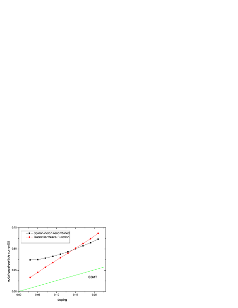
Figure 3: The quasiparticle charge of the nodal quasiparticle as a function of the hole concentration. The calculation is done on a $14\times 14$ lattice. $t^{{}^{\prime\prime}}=0$ is assumed in the calculation.

Since the property of the nodal quasiparticle is insensitive to the fine tuning of the Hamiltonian parameters, we will assume $t^{{}^{\prime\prime}}=0$ in the following calculations. The electromagnetic current operator of the t-J model in this assumption is given by

$$j_{x} = it\sum_{i,\sigma}(c^{\dagger}_{i,\sigma}c_{i+x,\sigma}-h.c.)$$ (24)

$$+ it^{\prime}\sum_{i,\sigma}(c^{\dagger}_{i,\sigma}c_{i+x+y,\sigma}-h.c.)$$

$$+ it^{\prime}\sum_{i,\sigma}(c^{\dagger}_{i,\sigma}c_{i+x-y,\sigma}-h.c.),$$

with $j_{y}$ given by a similar expression. In the slave Boson mean field theory, the current can be easily found to be given by $\vec{j}=x\nabla_{\mathrm{k}}\epsilon_{\mathrm{k}}$, where $\epsilon_{\mathrm{k}}$ is the mean field dispersion of the quasiparticle. Thus in the slave Boson mean field theory, the quasiparticle charge is proportional to the hole density $x$.

The quasiparticle current calculated from our variational wave function is shown in Fig.3 in which the result is compared with the predictions of the slave Boson mean field theory and the Gutzwiller projected variational wave function $|\mathrm{k},\sigma\rangle$. Unlike prediction of the mean field theory and the Gutzwiller projection scheme, the quasiparticle charge calculated from our wave function approaches to a finite value in the half filling limit. A non-vanishing quasiparticle charge, which is consistent with experimental observation in underdoped cuprates, constitutes the main achievement of the present theory.

IV.3 C. The quasiparticle weight and the nodal-antinodal dichotomy

In the slave Boson mean field theory, the quasiparticle weight is given by $Z_{\mathrm{k}}=xv^{2}_{\mathrm{k}}$. Thus, $Z_{\mathrm{k}}$ is isotropic on the underlying Fermi surface and increases with the excitation energy below the Fermi surface. Apart from some detailed difference in the doping dependence, the mean field predictions on the quasiparticle weight are to a large extent inherited by the Gutzwiller projected wave function $|\mathrm{k},\sigma\rangle$. However, the increase of the quasiparticle weight with excitation energy is obviously at odds with the experimental observations and our physical intuitions. At the same time, measurements have detected large anisotropy in the quasiparticle weight on the underlying Fermi surface in the underdoped cuprates. These two points constitute the main problems with the Gutzwiller projected wave function $|\mathrm{k},\sigma\rangle$.

To see if the backflow effect can cure these problems of $|\mathrm{k},\sigma\rangle$, we have calculated the quasiparticle weight from $|\mathrm{k},\sigma\rangle_{\mathrm{scr}}$ as a function of momentum. The quasiparticle weight in the present theory reads

$$Z_{\mathrm{k}}=\frac{\left|{}_{0}\langle\mathrm{k},\sigma|\mathrm{k},\sigma\rangle_{\mathrm{scr}}\right|^{2}}{\langle\Psi|\Psi\rangle}.$$ (25)

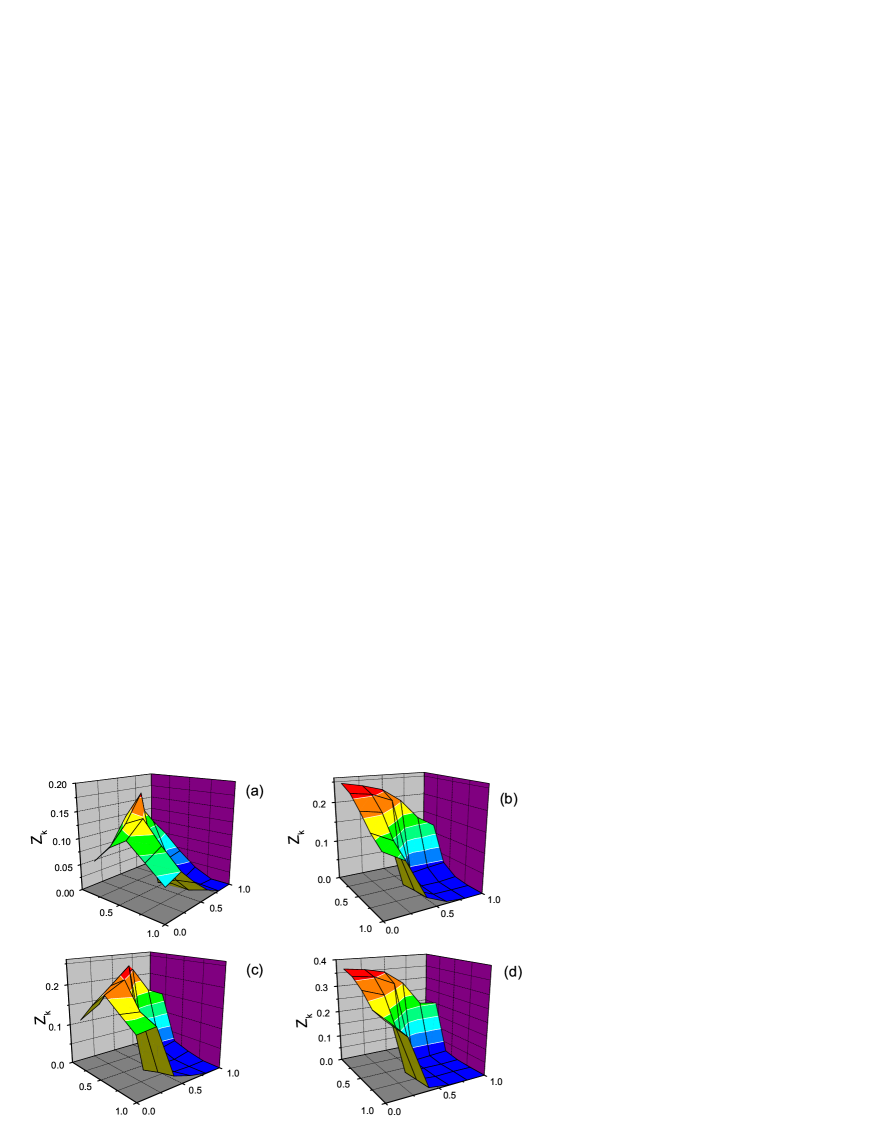
Figure 4: The quasiparticle weight in the first quadrant of the Brillouin zone for $t^{{}^{\prime\prime}}=0.2t$ calculated from the spin-charge recombined wave function((a) and (c)) and the Gutzwiller projected wave function((b) and (d)) at $x=6\%$((a) and (b)) and $x=14\%$((c) and (d)). The calculation is done on a $10\times 10$ lattice.

As the properties of the off-nodal quasiparticles are sensitive to the Hamiltonian parameters, we will present results calculated for both the $t^{{}^{\prime\prime}}=0.2t$ and $t^{{}^{\prime\prime}}=0$ case. The results for $t^{{}^{\prime\prime}}=0.2t$ is shown in Fig.5. Unlike the Gutzwiller projected wave function, our variational wave function predicts a quasiparticle weight that peaks on the Fermi surface. At the same time, the quasiparticle weight is anisotropic on the Fermi surface. The anisotropy is found to increases with decreasing doping and at $x=6\%$ the quasiparticle weight in the nodal region is almost three times larger than that in the antinodal region. These predictions of our theory resemble closely the experimental observations.

However, the anisotropy of the quasiparticle weight on the Fermi surface is not a generic property of our theory, but depends on fine tuning of Hamiltonian parameters. In Fig.6 we show the quasiparticle weight calculated with $t^{{}^{\prime\prime}}=0$. The anisotropy of the quasiparticle weight on the Fermi surface is found to be much smaller than that calculated with $t^{{}^{\prime\prime}}=0.2t$. Thus, in our theory the nodal-antinodal dichotomy is not a generic consequence of the spin-charge recombination effect, but depends on fine tuning of Hamiltonian parameters. The same conclusion is also reached by the variational calculation based on the dopon-spinon formalismRan .

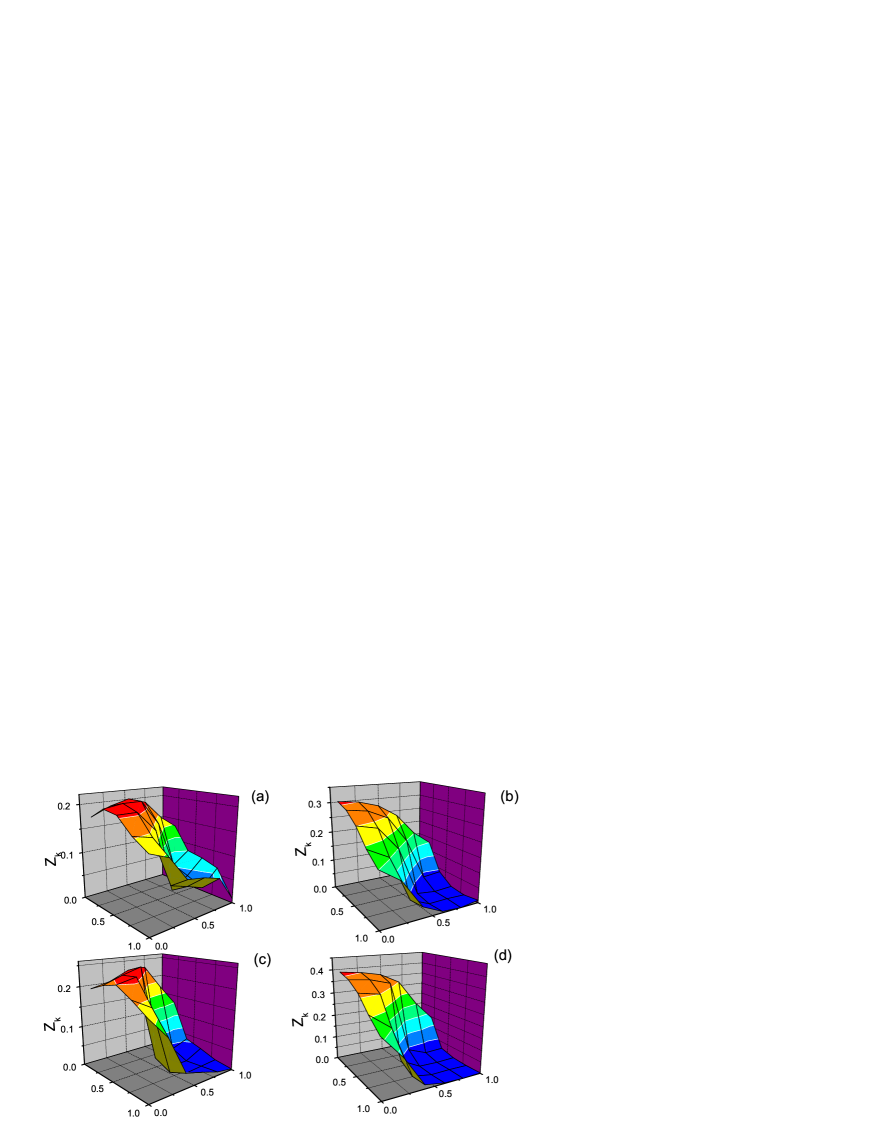
Figure 5: The quasiparticle weight in the first quadrant of the Brillouin zone for $t^{{}^{\prime\prime}}=0$ calculated from the spin-charge recombined wave function((a) and (c)) and the Gutzwiller projected wave function((b) and (d)) at $x=6\%$((a) and (b)) and $x=14\%$((c) and (d)). The calculation is done on a $10\times 10$ lattice.

V V. Discussions

In this work we have studied the consequence of the spin-charge recombination effect on the quasiparticle properties of the high-T_c cuprates. The spin-charge recombination effect, which can be interpreted as a backflow effect between the spinon and the holon degree of freedoms, originates from the no double occupancy constraint of the system. We find such a backflow effect will induce spinon-holon bound state and will cause qualitative changes in the quasiparticle properties.

In the Gutzwiller projected wave function, the no double occupancy constraint is enforced by hand. However, such a posteriorly enforced projection can not account for the full effect of the local constraint. Especially, the kinematic effect of such a constraint on the motion of the spinon and holon, namely the backflow effect, is totally beyond the reach of such a description. In the effective field theory context, the Gutzwiller projection amounts to integration of the temporal component of the gauge fluctuation with the spatial component of the gauge fluctuation totally untouched. Such a unbalanced nature of the treatment of the gauge fluctuation explains the qualitative similarity between the predictions made by the mean field theory and the Gutzwiller projected wave function.

The most remarkable consequence of the backflow effect on the quasiparticle properties is the modification of its electrodynamic response kernel. In the mean field theory, in which the motion of the spinon and holon is independent of each other, a quasiparticle carries a charge of $x$ through the holon condensate. The vanishing of the quasiparticle charge in the half filling limit predicted by the mean field theory is inherited by the Gutzwiller projected wave function. After the backflow effect correction, the spinon and the holon form bound state. The holon dragged by the spinon in such a composite object contributes a nonvanishing charge to the quasiparticle even in the half filling limit. It should be emphasized that this is generic consequence of the backflow effect and does not depends on fine tuning of Hamiltonian parameters.

The backflow effect can also provide a potential mechanism for the experimental observation of nodal-antinodal dichotomy and at the same time result in a quasiparticle weight that decreases with increasing excitation energy, as would be expected from general physical arguments. However, before making serious comparisons with experiments, it should be kept in mind that unlike the nodal quasiparticles, the off-nodal quasiparticles are in general sensitive to the fine tuning of Hamiltonian parameters. In particular, we find the anisotropy of the quasiparticle weight on the Fermi surface depends crucially on the value of $t^{{}^{\prime\prime}}$. We thus can not exclude the possibility that some other more generic mechanism is responsible for the observed nodal-antinodal dichotomy.

Finally, we note that the backflow effect will also cause renormalization of the ground state. In our calculation, we have assumed implicitly that such a renormalization is not strong enough to induce Fermi surface reconstruction, in which case our calculation would be totally invalid. In the absence of the Fermi surface reconstruction, such a renormalization effect on the ground state can in principle be taken into account in our theory to arrive at a more consistent description of the quasiparticle properties. When the backflow effect is strong enough to cause Fermi surface reconstruction, there arises the interesting and exotic possibility of forming a small Fermi pocket without any symmetry breaking. An important problem then is whether the small Fermi pocket has a quantized volume. We leave these issues to future study.

Tao Li is supported by NSFC Grant No. 10774187 and National Basic Research Program of China No. 2007CB925001, Fan Yang is grateful for the NSFC Grant No.10704008.

VI Appdenix A

In this appendix, we show the rank of the basis functions $|\mathrm{k},\mathrm{q},\sigma\rangle$ is lower than that of the mean field states $\gamma^{\dagger}_{\mathrm{k}-\mathrm{q},\sigma}b^{\dagger}_{\mathrm{q}}|\mathrm{SBMF}\rangle$ by one. This can be shown by proving the following identity

$$\sum_{\mathrm{q}}u_{\mathrm{k}-\mathrm{q}}|\mathrm{k},\mathrm{q},\sigma\rangle=0,$$ (26)

in which $u_{\mathrm{k}}=\frac{1}{2}(1-\frac{\xi_{\mathrm{k}}}{E_{\mathrm{k}}})$.

Using the Bogliubov transformation $f^{\dagger}_{\mathrm{k}\sigma}=u_{\mathrm{k}}\gamma^{\dagger}_{\mathrm{k}\sigma}+v_{\mathrm{k}}\gamma_{-\mathrm{k},\bar{\sigma}}$, we have $u_{\mathrm{k}-\mathrm{q}}\gamma^{\dagger}_{\mathrm{k}-\mathrm{q},\sigma}=f^{\dagger}_{\mathrm{k}-\mathrm{q},\sigma}-v_{\mathrm{k}-\mathrm{q}}\gamma_{-\mathrm{k}+\mathrm{q},\bar{\sigma}}$. As $\gamma_{-\mathrm{k}+\mathrm{q},\bar{\sigma}}|f-\mathrm{BCS}\rangle=0$, we have

$$\sum_{\mathrm{q}}u_{\mathrm{k}-\mathrm{q}}|\mathrm{k},\mathrm{q},\sigma\rangle$$ (27)

$$= \sum_{\mathrm{q}}\mathrm{P}_{N_{h}+1}\mathrm{P}_{\mathrm{s}}f^{\dagger}_{\mathrm{k}-\mathrm{q},\sigma}b^{\dagger}_{\mathrm{q}}|\mathrm{SBMF}\rangle$$

$$= \sum_{i}\mathrm{P}_{N_{h}+1}\mathrm{P}_{\mathrm{s}}f^{\dagger}_{i,\sigma}b^{\dagger}_{i}|\mathrm{SBMF}\rangle$$

$$= 0,$$

in which the no double occupancy constraint has been used in the final step.

VII Appdenix B

In this appendix, we derive the expression for the electron spectral function in the approximation that $|\mathrm{k,q},\sigma\rangle$ form a complete set for the description of the quasiparticle excitation and show that the spectral function so calculated does satisfy the sum rule.

A bare hole created in the ground state is given by $|\mathrm{k},\sigma\rangle_{0}=c_{\mathrm{k},\sigma}\mathrm{P}_{N_{e}}\mathrm{P}_{\mathrm{G}}|\mathrm{BCS}\rangle$. Written in terms of the slave particles, it reads

$$|\mathrm{k},\sigma\rangle_{0}=\sum_{\mathrm{q}}\mathrm{P}_{N_{h}+1}\mathrm{P}_{\mathrm{s}}f_{\mathrm{k-q},\sigma}b^{\dagger}_{\mathrm{q}}|\mathrm{SBMF}\rangle=\sum_{\mathrm{q}}\phi^{0}_{\mathrm{q}}|\mathrm{k,q},\sigma\rangle,$$ (28)

in which $\phi^{0}_{\mathrm{q}}=v_{\mathrm{k-q}}$. In the derivation we have used the fact that $\mathrm{P}_{\mathrm{s}}$ and $f_{i,\sigma}b^{\dagger}_{i}$ commute with each other.

Assuming that $|\mathrm{k,q},\sigma\rangle$ form a complete set, the electronic spectral function can then be calculated as

$$A(\mathrm{k},\omega)=\sum_{n}|_{0}\langle\mathrm{k},\sigma|\mathrm{k},\sigma\rangle_{n}|^{2}\delta(\omega-(\mathrm{E}_{\mathrm{k},n}-\mathrm{E}_{g})),$$ (29)

in which $|\mathrm{k},\sigma\rangle_{n}$ denotes the $n-$th eigenvector of Eq.(15) and $\mathrm{E}_{\mathrm{k},n}$ is corresponding eigenvalue. $\mathrm{E}_{g}$ is the variational ground state energy. We thus have

$$A(\mathrm{k},\omega)=\sum_{n,\mathrm{q,q^{\prime}}}|\phi^{0*}_{\mathrm{q}}\mathrm{O}_{\mathrm{q,q^{\prime}}}\phi^{n}_{\mathrm{q^{\prime}}}|^{2}\delta(\omega-(\mathrm{E}_{\mathrm{k},n}-\mathrm{E}_{g})),$$ (30)

in which $\phi^{n}_{\mathrm{q}}$ is the $n-$th eigenvector of Eq.(15) and satisfies the following orthonormal condition

$$\sum_{\mathrm{q,q^{\prime}}}\phi^{n*}_{\mathrm{q}}\mathrm{O}_{\mathrm{q,q^{\prime}}}\phi^{m}_{\mathrm{q^{\prime}}}=\delta_{n,m}.$$ (31)

The electronic spectral function so obtained satisfy the sum rule $\int d\omega A(\mathrm{k},\omega)=\langle\Psi|c^{\dagger}_{\mathrm{k},\sigma}c_{\mathrm{k},\sigma}|\Psi\rangle$. In fact, from Eq.(5) we have

$$\int d\omega A(\mathrm{k},\omega) = \sum_{n}|_{0}\langle\mathrm{k},\sigma|\mathrm{k},\sigma\rangle_{n}|^{2}=_{0}\langle\mathrm{k},\sigma|\mathrm{k},\sigma\rangle_{0}$$ (32)

$$= \langle\Psi|c^{\dagger}_{\mathrm{k},\sigma}c_{\mathrm{k},\sigma}|\Psi\rangle,$$

where we have used the fact that $|\mathrm{k},\sigma\rangle_{n}$ forms a complete set in the space spanned by $|\mathrm{k,q},\sigma\rangle$.

References

- (1) A. Damascelli, Z. X. Shen and Z. Hussain, Rev. Mod. Phys. 75, 473 (2003).
- (2) H. Ding, T. Yokoya, J. C. Campuzano, T. Takahashi, M. Randeria, M. R. Norman, T. Mochiku, K. Kadowaki and J. Giapintzakis, Nature. Vol 382, 51 (1996) .
- (3) Y. Kohsaka, C. Taylor, K. Fujita, A. Schmidt, C. Lupien, T. Hanaguri, M. Azuma,. M. Takano, H. Eisaki, H. Takagi, S. Uchida, and J. C. Davis, Science 315, 1380 (2007).
- (4) A.Kanigel et al., Nature Phys. Vol 2, 447 (2006).
- (5) M. Le Tacon, A. Sacuto, A. Georges, G. Kotliar, Y. Gallais, D. Colson and A. Forget, Nature Physics, 2, 537(2006).
- (6) K. Tanaka, W. S. Lee, D. H. Lu, A. Fujimori, T. Fujii, Risdiana, I. Terasaki, D. J. Scalapino, T. P. Devereaux, Z. Hussain and Z.-X. Shen, Science, 314, 1910(2006).
- (7) N. Doiron-Leyraud, C. Proust, D. LeBoeuf, J. Levallois, J.-B. Bonnemaison, R. Liang, D. A. Bonn, W. N. Hardy, and L. Taillefer, Nature 447, 565 (2007).
- (8) P.A. Lee, N. Nagaosa and X-G Wen, Rev. Mod. Phys. 78, 17 (2006).
- (9) T. Senthil, M. Vojta and S. Sachdev, Phys. Rev. B 69, 035111 (2004).
- (10) A. Paramekanti and A. Vishwanath, Phys.Rev. B 70, 245118(2004).
- (11) W. Rantner and X.G. Wen, Phys. Rev. Lett. 85, 3692 (2000).
- (12) For a review on this subject, see B. Edegger, V.N. Muthukumar, C. Gros, Adv. Phys. 56, 927 (2007).
- (13) P.W. Andeson and N.P. Ong, Cond-mat/0405518.
- (14) M. Randeria, R. Sensarma, N. Trivedi, and F.C. Zhang, Phys. Rev. Lett. 95, 137001 (2005).
- (15) S. Yunoki, Phys. Rev. B 72, 092505 (2005).
- (16) C. Gros, B. Edegger, V.N. Muthukumar, P.W. Anderson, PNAS 103, 14298 (2006); B. Edegger, V.N. Muthukumar, C. Gros, P.W. Anderson,Phys. Rev. Lett. 96, 207002 (2006); B. Edegger, N. Fukushima, C. Gros, V.N. Muthukumar,Phys. Rev. B 72, 134504 (2005).
- (17) C.P. Nave, D.A.Ivanov and P.A. Lee, Phys. Rev. B 73, 104502 (2006).
- (18) C.T. Shih, T.K. Lee, R. Eder, C.Y. Mou, and Y.C. Chen, Phys. Rev. Lett. 92, 227002 (2004).
- (19) S. Yunoki, E. Dagotto, and S. Sorella, Phys. Rev. Lett. 94, 037001 (2005).
- (20) H.Y. Yang, F. Yang, Y. J. Jiang and T. Li, J. Phys.: Condens. Matter 19 016217, (2007).
- (21) Xiao-Gang Wen and Patrick A. Lee, Phys. Rev. Lett. 76, 503 (1996).
- (22) P.A. Lee, N. Nagaosa, T.K. Ng, and X.G. Wen, Phys. Rev. B 57, 6003 (1998).
- (23) Y. Ran and X. G. Wen, arXiv:cond-mat/0609620.
- (24) T. Li and F. Yang, Phys. Rev. B 81, 214509 (2010).