Syzygy gap fractals—I.
Some structural results and an upper bound

Abstract

$\Bbbk$ is a field of characteristic $p>0$, and $\ell_{1},\ldots,\ell_{n}$ are linear forms in $\Bbbk[x,y]$. Intending applications to Hilbert–Kunz theory, to each triple $C=(F,G,H)$ of nonzero homogeneous elements of $\Bbbk[x,y]$ we associate a function $\delta_{C}$ that encodes the “syzygy gaps” of $F^{q}$, $G^{q}$, and $H^{q}\ell_{1}^{a_{1}}\cdots\ell_{n}^{a_{n}}$, for all $q=p^{e}$ and $a_{i}\leq q$. These are close relatives of functions introduced in $p$-Fractals and power series—I [P. Monsky, P. Teixeira, $p$-Fractals and power series—I. Some 2 variable results, J. Algebra 280 (2004) 505–536]. Like their relatives, the $\delta_{C}$ exhibit surprising self-similarity related to “magnification by $p$,” and knowledge of their structure allows the explicit computation of various Hilbert–Kunz functions.

We show that these “syzygy gap fractals” are determined by their zeros and have a simple behavior near their local maxima, and derive an upper bound for their local maxima which has long been conjectured by Monsky. Our results will allow us, in a sequel to this paper, to determine the structure of the $\delta_{C}$ by studying the vanishing of certain determinants.

1 Introduction

Let $\Bbbk$ be a field of characteristic $p>0$ and $A=\Bbbk[x,y]$. Let $F$, $G$, and $H\in A$ be nonzero homogeneous polynomials with no common factor. The module of syzygies of $F$, $G$, and $H$ is free on two homogeneous generators; let $\alpha\geq\beta$ be their degrees. We define $\delta(F,G,H)=\alpha-\beta$; this is the syzygy gap of $F$, $G$, and $H$. Syzygy gaps were introduced by Han [3], were studied by the author in his thesis [10], and have since made scattered appearances in the literature [2, 4, 7].

This paper is concerned with a family of functions introduced in [10], defined in terms of syzygy gaps. Fix pairwise prime linear forms $\ell_{1},\ldots,\ell_{n}\in A$, and let $C=(F,G,H)$ be a triple of nonzero homogeneous elements of $A$ such that $F$, $G$, and $H\ell_{1}\cdots\ell_{n}$ have no common factor. Let $\mathscr{I}=[0,1]\cap\mathbb{Z}[1/p]$. We define $\delta_{C}:\mathscr{I}^{n}\to\mathbb{Q}$ as follows: for each $q=p^{e}$ and ${\mathbf{{a}}}=(a_{1},\ldots,a_{n})\in\mathbb{Z}^{n}$ with $0\leq a_{i}\leq q$, we set

$$\delta_{C}\left(\frac{{\mathbf{{a}}}}{q}\right)=\frac{1}{q}\cdot\delta(F^{q},G^{q},H^{q}\ell_{1}^{a_{1}}\cdots\ell_{n}^{a_{n}}).$$

A two-dimensional “slice” of one such function is shown in Figure 1, as a relief plot—zeros are shown in black, and other values are encoded by color (higher value $\leftrightarrow$ lighter color).

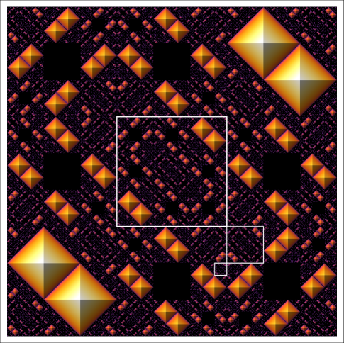
Figure 1: A syzygy gap fractal in characteristic 3

The white squares highlight three smaller copies of the plot contained within itself. The $\delta_{C}$ often bear this kind of self-similarity, and if $\Bbbk$ is finite they are $p$-fractals, in the sense of [8]. As such, they can be characterized by a finite set of values and a finite set of functional equations—the “magnification rules”—that prescribe how pieces patch together to form the function.

The “syzygy gap fractals” $\delta_{C}$ are closely related to functions $\varphi_{I}:\mathscr{I}^{n}\to\mathbb{Q}$ introduced (in a more general setting) by Monsky and the author in [8]. Restricting to the situation at hand we let $I={\langle{F,G}\rangle}:H$ and define, for ${\mathbf{{a}}}$ and $q$ as above,

$$\varphi_{I}\left(\frac{{\mathbf{{a}}}}{q}\right)=\frac{1}{q^{2}}\cdot\deg{\langle{I^{[q]},\ell_{1}^{a_{1}}\cdots\ell_{n}^{a_{n}}}\rangle},$$

where $I^{[q]}={\langle{u^{q}:u\in I}\rangle}$ and $\deg$ denotes the degree or colength of an ideal. Then $\delta_{C}^{2}$ and $4\varphi_{I}$ differ by a polynomial in the coordinate functions (see Eq. (4) in Section 3).

In [9] the $\varphi_{I}$ are used in the proof of rationality and computation of the Hilbert–Kunz series and multiplicities of power series of the form $f_{1}(x_{1},y_{1})+\cdots+f_{m}(x_{m},y_{m})$ with coefficients in a finite field. More specifically, the “$p$-fractalness” of the $\varphi_{I}$, established in [8], gives us the rationality result, while knowledge of the magnification rules for those functions (when available) allows us to explicitly compute related Hilbert–Kunz series and multiplicities. In the present paper we focus on the homogeneous case and find properties of the syzygy gap fractals $\delta_{C}$ that will help in those explicit calculations.

The main results of this paper concern the zeros and local maxima of the $\delta_{C}$. We prove that these functions (when nontrivial) are determined by their zeros:

Theorem I.

Let ${\mathcal{Z}}=\{{\mathbf{{z}}}\in\mathscr{I}^{n}\,|\,\delta_{C}({\mathbf{{z}}})=0\}$.

• If ${\mathcal{Z}}$ is empty, then $\delta_{C}$ is linear; it takes on a minimum value at a corner ${\mathbf{{u}}}$ of $\mathscr{I}^{n}$ and, at each ${\mathbf{{t}}}\in\mathscr{I}^{n}$,

  $$\delta_{C}({\mathbf{{t}}})=\delta_{C}({\mathbf{{u}}})+d({\mathbf{{t}}},{\mathbf{{u}}}),$$

  where $d({\mathbf{{t}}},{\mathbf{{u}}})$ is the taxi-cab distance between ${\mathbf{{t}}}$ and ${\mathbf{{u}}}$.

• If ${\mathcal{Z}}$ is nonempty then $\delta_{C}({\mathbf{{t}}})$ is the taxi-cab distance from ${\mathbf{{t}}}$ to the set ${\mathcal{Z}}$, for all ${\mathbf{{t}}}\in\mathscr{I}^{n}$.

This result has some interesting consequences that will be explored in a sequel to this paper: since the vanishing of the syzygy gap is tied to the vanishing of a certain determinant in the coefficients of the polynomials, we shall use those determinants in the investigation of the $\delta_{C}$. We shall prove that the $\delta_{C}$ are completely determined by finitely many such determinants, and this will give us a powerful tool for determining magnification rules, thus allowing the explicit (and even automatic) calculation of various Hilbert–Kunz series and multiplicities.

Related to Theorem I is our next result, which shows that each local maximum of $\delta_{C}$ determines the behavior of the function on a certain neighborhood:

Theorem II.

Let $q$ be a power of $p$, and let ${{\mathcal{X}}_{q}}$ be the set consisting of all points of $\mathscr{I}^{n}$ with denominator $q$. Suppose the restriction of $\delta_{C}$ to ${\mathcal{X}}_{q}$ attains a “local maximum” at ${\mathbf{{u}}}$, in the sense that the values of $\delta_{C}$ at all points of ${\mathcal{X}}_{q}$ adjacent to ${\mathbf{{u}}}$ are smaller than $\delta_{C}({\mathbf{{u}}})$. Then

$$\delta_{C}({\mathbf{{t}}})=\delta_{C}({\mathbf{{u}}})-d({\mathbf{{t}}},{\mathbf{{u}}}),$$

for all ${\mathbf{{t}}}\in\mathscr{I}^{n}$ with $d({\mathbf{{t}}},{\mathbf{{u}}})\leq\delta_{C}({\mathbf{{u}}})$. In particular, $\delta_{C}$ is piecewise linear on that region, and has a local maximum at ${\mathbf{{u}}}$ in the usual sense.

Theorem II plays a major role in understanding the structure of the $\delta_{C}$, and is fundamental in the proof of the last of our results, which shows the existence of a certain upper bound for the $\delta_{C}$ at their local maxima:

Theorem III.

Suppose $\delta_{C}$ has a local maximum at ${\mathbf{{a}}}/q$, where $q>1$ and some $a_{i}$ is not divisible by $p$. Then

$$\delta_{C}\left(\frac{{\mathbf{{a}}}}{q}\right)\leq\frac{n-2}{q}.$$

This bound has long been conjectured by Monsky; in [7] he proved it holds when $C=(x,y,1)$. The approach used here follows closely an alternate, unpublished proof by Monsky of his result from [7], where he gets information on the local maxima of $\delta_{C}$ by combining a theorem of Trivedi [11, Theorem 5.3] on the Hilbert–Kunz multiplicity of a certain projective plane curve and a formula expressing that same multiplicity in terms of a continuous extension of $\delta_{C}$. Here we combine results of Brenner [1, Corollary 4.4] and Trivedi [11, Lemma 5.2] and follow essentially the same track to get to the stronger result, modulo some technical obstacles.

This paper is structured as follows. In Section 2 we prove some properties of syzygy gaps independent of the characteristic. Starting in Section 3 we restrict our attention to positive characteristic; we introduce the functions $\delta_{C}$ and look at various examples, and in Section 4 we prove Theorems I and II. In Section 5 we introduce operators on the “cells” $C=(F,G,H)$ that are mirrored by “magnifications” and “reflections” on the corresponding functions. While the “$p$-fractalness” of the $\delta_{C}$ when $\Bbbk$ is finite is not directly relevant to this paper, it follows without much effort from the machinery introduced in Section 5, so we present a proof in that section. Finally, in Section 6 we prove Theorem III.

Throughout this paper $p$ denotes a prime number and (lower-case) $q$ is used exclusively for powers of $p$; $\Bbbk$ is a field, assumed everywhere but in Section 2 to be of characteristic $p$; $\mathscr{I}$ is the set of rational numbers in $[0,1]$ whose denominators are powers of $p$.

2 Syzygy gaps

Throughout this section $\Bbbk$ is a field of arbitrary characteristic, and $F$, $G$, and $H$ are nonzero homogeneous elements of $A=\Bbbk[x,y]$. By the Hilbert Syzygy Theorem, the module of syzygies of $(F,G,H)$, denoted by $\operatorname{Syz}(F,G,H)$, is free on two homogeneous generators.

Definition 2.1.

The syzygy gap of $F$, $G$, and $H$ is the nonnegative integer $\delta=n-m$, where $m\leq n$ are the degrees of the generators of $\operatorname{Syz}(F,G,H)$.

In this section we prove some general properties of syzygy gaps that are characteristic independent. Some of these appeared in [7], but are included here, with proofs, for completeness. Our first result relates the syzygy gap to the degree of the ideal ${\langle{F,G,H}\rangle}$ when this degree is finite.

Proposition 2.2.

Let $F$, $G$, and $H\in\Bbbk[x,y]$ be nonzero homogeneous polynomials with no common factor, of degrees $d_{1}$, $d_{2}$, and $d_{3}$, and let $\delta$ be their syzygy gap. Then

$$4\deg{\langle{F,G,H}\rangle}=Q(d_{1},d_{2},d_{3})+\delta^{2},$$

where

$$Q(d_{1},d_{2},d_{3})=2(d_{1}d_{2}+d_{1}d_{3}+d_{2}d_{3})-{d_{1}}^{2}-{d_{2}}^{2}-{d_{3}}^{2}.$$

Proof 1.

Let $m$ and $n$ be as in Definition 2.1. $A/{\langle{F,G,H}\rangle}$ has a graded free resolution

$$0\rightarrow A(-m)\oplus A(-n)\rightarrow\bigoplus_{i=1}^{3}A(-d_{i})\rightarrow A\rightarrow A/{\langle{F,G,H}\rangle}\rightarrow 0,$$

so the Hilbert series of $A/{\langle{F,G,H}\rangle}$ is

$$h(t)=\frac{1-t^{d_{1}}-t^{d_{2}}-t^{d_{3}}+t^{m}+t^{n}}{(1-t)^{2}}.$$

Since $F$, $G$, and $H$ have no common factor, $h(1)=\deg{\langle{F,G,H}\rangle}$ is finite. Differentiating $(1-t)^{2}h(t)$ and setting $t=1$ we find

$$m+n=d_{1}+d_{2}+d_{3}.$$ (1)

Differentiating $(1-t)^{2}h(t)$ twice and setting $t=1$ we get

$$2h(1)=-d_{1}(d_{1}-1)-d_{2}(d_{2}-1)-d_{3}(d_{3}-1)+m(m-1)+n(n-1),$$

and the result follows easily. ∎

Eq. (1) shows that $\delta=d_{1}+d_{2}+d_{3}-2m$; this suggests the following definition:

Definition 2.3.

$\delta(F,G,H)=\deg F+\deg G+\deg H-2m(F,G,H),$ where $m(F,G,H)$ is the least degree of a nontrivial syzygy of $(F,G,H)$.

Remark 2.4.

If $F$, $G$, and $H$ have no common factor, $\delta(F,G,H)$ is just the syzygy gap of $F$, $G$, and $H$. In this case, Proposition 2.2 shows that $\delta(F,G,H)$ remains unchanged under any modification in the polynomials $F$, $G$, and $H$ that fixes their degrees and the ideal ${\langle{F,G,H}\rangle}$ or, more generally, that fixes $Q(\deg F,\deg G,\deg H)$ and $\deg{\langle{F,G,H}\rangle}$.

Remark 2.5.

If $d_{3}\geq d_{1}+d_{2}$ and $F$ and $G$ have no common factor, then $(G,-F,0)$ is a syzygy of minimal degree, and $\delta(F,G,H)=d_{3}-d_{1}-d_{2}.$

Proposition 2.6.

Let $P\in\Bbbk[x,y]$ be a nonzero homogeneous polynomial. Then

1. $\delta(PF,PG,PG)=\delta(F,G,H)+\deg P$;

2. $\delta(PF,PG,H)=\delta(F,G,H)$, whenever $P$ is prime to $H$.

Proof 2.

Let $d=\deg P$; then $\operatorname{Syz}(F,G,H)$ and $\operatorname{Syz}(PF,PG,PH)(d)$ coincide, and that gives the first identity. For the second identity, note that there is an injective map $\operatorname{Syz}(F,G,H)\to\operatorname{Syz}(PF,PG,H)(d)$ that sends $(\alpha,\beta,\gamma)$ to $(\alpha,\beta,P\gamma)$. If $P$ is prime to $H$ then this map is surjective as well; so $m(PF,PG,H)=m(F,G,H)+d$, and the identity follows easily. ∎

Proposition 2.7.

If $P\in\Bbbk[x,y]$ is a nonzero homogeneous polynomial, then

$$|\delta(F,G,PH)-\delta(F,G,H)|\leq\deg P.$$

Proof 3.

Let $d=\deg P$. There is a map $\operatorname{Syz}(F,G,H)\to\operatorname{Syz}(F,G,PH)(d)$, $(\alpha,\beta,\gamma)\mapsto(\alpha P,\beta P,\gamma)$; so $m(F,G,PH)\leq m(F,G,H)+d$. There is also a degree-preserving map $\operatorname{Syz}(F,G,PH)\to\operatorname{Syz}(F,G,H)$, $(\alpha,\beta,\gamma)\mapsto(\alpha,\beta,\gamma P)$; so $m(F,G,H)\leq m(F,G,PH)$. The desired inequality follows at once. ∎

If $\ell\in\Bbbk[x,y]$ is a linear form, $\delta(F,G,H)$ and $\delta(F,G,H\ell)$ cannot be equal, since they have different parities. So, by the previous proposition,

$$\delta(F,G,\ell H)=\delta(F,G,H)\pm 1.$$

We can make this more precise:

Proposition 2.8.

Suppose $F$, $G$, and $H$ have no common factor, and let $\ell\in\Bbbk[x,y]$ be a linear form. If $\delta(F,G,H)>0$ and $(\alpha,\beta,\gamma)$ is a syzygy of $(F,G,H)$ of minimal degree, then $\delta(F,G,\ell H)=\delta(F,G,H)+1$ if $\ell$ divides $\gamma$, and $\delta(F,G,\ell H)=\delta(F,G,H)-1$ otherwise.

Proof 4.

If $\ell$ divides $\gamma$, then $(\alpha,\beta,\gamma/\ell)$ is an element of $\operatorname{Syz}(F,G,\ell H)$ of minimal degree; so $m(F,G,\ell H)=m(F,G,H)$, giving $\delta(F,G,\ell H)=\delta(F,G,H)+1$. If $\ell$ does not divide $\gamma$, then we claim that $(\alpha\ell,\beta\ell,\gamma)$ is an element of $\operatorname{Syz}(F,G,\ell H)$ of minimal degree. In fact, suppose there exists $(\alpha^{\prime},\beta^{\prime},\gamma^{\prime})\in\operatorname{Syz}(F,G,\ell H)$ of degree $m=m(F,G,H)$. Then $(\alpha^{\prime},\beta^{\prime},\gamma^{\prime}\ell)\in\operatorname{Syz}(F,G,H)$ has degree $m$, and since the syzygy gap of $F$, $G$, and $H$ is nonzero, $(\alpha^{\prime},\beta^{\prime},\gamma^{\prime}\ell)$ must be a constant multiple of $(\alpha,\beta,\gamma)$, contradicting the assumption that $\ell$ does not divide $\gamma$. So $m(F,G,\ell H)=m(F,G,H)+1$, and $\delta(F,G,\ell H)=\delta(F,G,H)-1$. ∎

Proposition 2.9.

Let $\ell\in\Bbbk[x,y]$ be a linear form, and suppose $F$, $G$, and $\ell H$ have no common factor. If $\delta(F,G,H)$ and $\delta(F,G,\ell^{2}H)$ are both greater than $\delta(F,G,\ell H)$, then $\delta(F,G,\ell H)=0$.

Proof 5.

Multiplication by $\ell$ gives us a surjective map

$${\langle{F,G,H}\rangle}/{\langle{F,G,\ell H}\rangle}\ \stackrel{{\scriptstyle\ell}}{{\longrightarrow}}\ {\langle{F,G,\ell H}\rangle}/{\langle{F,G,\ell^{2}H}\rangle},$$

so $\deg{\langle{F,G,\ell H}\rangle}-\deg{\langle{F,G,H}\rangle}\geq\deg{\langle{F,G,\ell^{2}H}\rangle}-\deg{\langle{F,G,\ell H}\rangle}$. Using Proposition 2.2 we obtain

$$\delta(F,G,H)^{2}+\delta(F,G,\ell^{2}H)^{2}\leq 2\cdot\delta(F,G,\ell H)^{2}+2.$$

But $\delta(F,G,H)=\delta(F,G,\ell^{2}H)=\delta(F,G,\ell H)+1$, so the inequality above implies that $\delta(F,G,\ell H)=0$. ∎

Proposition 2.10.

Let $\ell_{1}$ and $\ell_{2}$ be relatively prime linear forms, such that $F$, $G$ and $H\ell_{1}\ell_{2}$ have no common factor. Suppose that $\delta(F,G,H)=\delta(F,G,H\ell_{1}\ell_{2})$ and $\delta(F,G,H\ell_{1})=\delta(F,G,H\ell_{2})$. Then either $\delta(F,G,H)=0$ or $\delta(F,G,H\ell_{1})=0$.

Proof 6.

Suppose $\delta:=\delta(F,G,H)>0$, and let $(\alpha,\beta,\gamma)$ be a syzygy of $(F,G,H)$ of minimal degree $m$. We use Proposition 2.8 repeatedly. Since $\delta(F,G,H\ell_{1})=\delta(F,G,H\ell_{2})$, either both $\ell_{1}$ and $\ell_{2}$ divide $\gamma$, or neither one does. If both linear forms divided $\gamma$, then $(\alpha,\beta,\gamma/(\ell_{1}\ell_{2}))$ would be a syzygy of $(F,G,H\ell_{1}\ell_{2})$ of degree $m$ and we would have $\delta(F,G,H\ell_{1}\ell_{2})>\delta$, contradicting our hypothesis. So neither $\ell_{1}$ nor $\ell_{2}$ divides $\gamma$, and $\delta(F,G,H\ell_{1})=\delta(F,G,H\ell_{2})=\delta-1.$

Now $(\ell_{1}\alpha,\ell_{1}\beta,\gamma)$ is a syzygy of $(F,G,H\ell_{1})$ of minimal degree, and since $\ell_{2}$ does not divide $\gamma$ it must be the case that $\delta(F,G,H\ell_{1})=0$, since otherwise $\delta(F,G,H\ell_{1}\ell_{2})=\delta-2$, contradicting the hypothesis. ∎

3 Syzygy gap fractals

The properties of syzygy gaps so far discussed hold over arbitrary fields. In this section, and in the remainder of the paper, we assume that $\operatorname{char}\Bbbk=p>0$ and introduce a family of functions defined in terms of syzygy gaps. Once again $F$, $G$, and $H$ are nonzero homogeneous polynomials in $A=\Bbbk[x,y]$. If $(\alpha,\beta,\gamma)$ is a syzygy of $(F,G,H)$ of minimal degree, then $(\alpha^{p},\beta^{p},\gamma^{p})$ is a syzygy of $(F^{p},G^{p},H^{p})$ of minimal degree. It follows that

$$\delta(F^{p},G^{p},H^{p})=p\cdot\delta(F,G,H).$$ (2)

In what follows, we fix a positive integer $n$ and pairwise prime linear forms $\ell_{1},\ldots,\ell_{n}\in\Bbbk[x,y]$. For ease of notation we introduce the following shorthands, which will be used throughout the paper: $\ell=\prod_{i=1}^{n}\ell_{i}$, and for any nonnegative integer vector ${\mathbf{{a}}}=(a_{1},\ldots,a_{n})$, $\ell^{\mathbf{{a}}}=\prod_{i=1}^{n}\ell_{i}^{a_{i}}$.

Definition 3.11.

A cell (with respect to the linear forms $\ell_{1},\ldots,\ell_{n}$) is a triple ${\left({F,G,H}\right)}$ of nonzero homogeneous polynomials in $\Bbbk[x,y]$ such that $F$, $G$, and $H\ell$ have no common factor.

Let $C={\left({F,G,H}\right)}$ be a cell, $[q]=\{0,1,\ldots,q\}$, and ${\mathbf{{a}}}\in[q]^{n}$; we wish to understand how $\delta(F^{q},G^{q},H^{q}\ell^{\mathbf{{a}}})$ depends on $q$ and ${\mathbf{{a}}}$. Eq. (2) allows us to conveniently encode these syzygy gaps in a single function $\mathscr{I}^{n}\to\mathbb{Q}$, where $\mathscr{I}=[0,1]\cap\mathbb{Z}[1/p]$:

Definition 3.12.

To each cell $C={\left({F,G,H}\right)}$ we attach a function $\delta_{C}:\mathscr{I}^{n}\to\mathbb{Q}$ where

$$\delta_{C}\left(\frac{{\mathbf{{a}}}}{q}\right)=\frac{1}{q}\cdot\delta\left(F^{q},G^{q},H^{q}\ell^{\mathbf{{a}}}\right)$$

for any $q$ and any ${\mathbf{{a}}}\in[q]^{n}$. (Eq. (2) ensures that $\delta_{C}$ is well-defined.) We shall nickname these functions syzygy gap fractals, for reasons that will soon become apparent.

Remark 3.13.

In [8] Monsky and the author studied a closely related family of functions $\varphi_{I}$ associated to zero-dimensional ideals $I$ of $\Bbbk\llbracket x,y\rrbracket$. In what follows we shall explore this relation.

Let $C={\left({F,G,H}\right)}$ be a cell and $I={\langle{F,G}\rangle}:H$. Since ${\langle{F,G,\ell}\rangle}\subseteq{\langle{I,\ell}\rangle}$ and $F$, $G$, and $\ell$ have no common factor, $\deg{\langle{I,\ell}\rangle}<\infty$ and we can define the following function, as in [8]:

$$\varphi_{I}:\mathscr{I}^{n} \longrightarrow\mathbb{Q}$$

$$\frac{{\mathbf{{a}}}}{q} \longmapsto\frac{1}{q^{2}}\cdot\deg{\langle{I^{[q]},\ell^{\mathbf{{a}}}}\rangle}$$

Here $I^{[q]}$ denotes the $q$th Frobenius power of $I$, i.e., the ideal generated by the $q$th powers of the elements of $I$. To relate $\delta_{C}$ and $\varphi_{I}$ we define a similar function

$$\varphi_{C}:\mathscr{I}^{n} \longrightarrow\mathbb{Q}$$

$$\frac{{\mathbf{{a}}}}{q} \longmapsto\frac{1}{q^{2}}\cdot\deg{\langle{F^{q},G^{q},H^{q}\ell^{\mathbf{{a}}}}\rangle}$$

and start by relating $\varphi_{C}$ and $\delta_{C}$. Setting $d=\deg{\langle{F,G,H}\rangle}$ and $\delta=\delta(F,G,H)$, Proposition 2.2 gives

$$4\varphi_{C}({\mathbf{{t}}})=\delta_{C}^{2}({\mathbf{{t}}})+4d-\delta^{2}+2(\deg F+\deg G-\deg H)\sum_{i=1}^{n}{t_{i}}-\left(\sum_{i=1}^{n}t_{i}\right)^{2}.$$ (3)

To relate $\varphi_{I}$ and $\varphi_{C}$, note that for any ideal $J$ of $A$ and $f\in A$ we have $\deg J=\deg(J:f)+\deg{\langle{J,f}\rangle}$, and replacing $J$ with ${\langle{J,fg}\rangle}$, that becomes $\deg{\langle{J,fg}\rangle}=\deg{\langle{(J:f),g}\rangle}+\deg{\langle{J,f}\rangle}.$ Setting $J={\langle{F^{q},G^{q}}\rangle}$, $f=H^{q}$, $g=\ell^{\mathbf{{a}}}$, and dividing by $q^{2}$ we find that $\varphi_{C}=\varphi_{I}+\deg{\langle{F,G,H}\rangle}$. Together with Eq. (3), this gives

$$4\varphi_{I}({\mathbf{{t}}})=\delta_{C}^{2}({\mathbf{{t}}})-\delta^{2}+2(\deg F+\deg G-\deg H)\sum_{i=1}^{n}{t_{i}}-\left(\sum_{i=1}^{n}t_{i}\right)^{2}.$$ (4)

This, in turn, gives us the following result:

Proposition 3.14.

Let $C={\left({F,G,H}\right)}$ be a cell. Then the ideal ${\langle{F,G}\rangle}:H$ is generated by two homogeneous polynomials $U$ and $V$ such that $\delta_{C}=\delta_{\left({U,V,1}\right)}$.

Proof 7.

$\operatorname{Syz}(F,G,H)$ has two homogeneous generators, and their third components $U$ and $V$ generate ${\langle{F,G}\rangle}:H$. Since ${\langle{F,G}\rangle}\subseteq{\langle{U,V}\rangle}$, the polynomials $U$, $V$, and $\ell$ have no common factor, so ${\left({U,V,1}\right)}$ is a cell. The generators of $\operatorname{Syz}(F,G,H)$ have degrees $\deg U+\deg H$ and $\deg V+\deg H$, so Eq. (1) shows that $\deg U+\deg V=\deg F+\deg G-\deg H$. Noting that $\delta(U,V,1)=|\deg U-\deg V|=\delta(F,G,H)$, the result is obtained by replacing $C={\left({F,G,H}\right)}$ with ${\left({U,V,1}\right)}$ in Eq. (4) and comparing with the same equation in its original form. ∎

Remark 3.15.

If the image of the colon ideal $I={\langle{F,G}\rangle}:H$ in $\bar{A}=A/{\langle{\ell}\rangle}$ is not principal, then $\delta_{C}=\delta_{\left({U,V,1}\right)}$ for any pair of generators $U$ and $V$ of $I$. This is not the case otherwise. In fact, if the image of ${\langle{U,V}\rangle}$ is principal in $\bar{A}$, suppose the image of $U$ is the generator. We can modify $V$ by a multiple of $U$, without affecting $\delta_{\left({U,V,1}\right)}$, to assume that $V=W\ell$ for some $W$. Then Proposition 2.6 shows that $\delta_{\left({U,V,1}\right)}({\mathbf{{a}}}/q)=q^{-1}\cdot\delta(U^{q},W^{q}\ell^{q},\ell^{\mathbf{{a}}})=q^{-1}\cdot\delta(U^{q},W^{q}\ell^{q}/\ell^{\mathbf{{a}}},1)=|\deg V-\deg U-\sum_{i=1}^{n}a_{i}/q|$, which depends on the degree of $V$.

Remark 3.16.

In view of Proposition 3.14, as far as the study of the functions $\delta_{C}$ is concerned we can always assume that the cells have the form ${\left({F,G,1}\right)}$, which we shall often abbreviate by ${\left({F,G}\right)}$.

Example 3.17.

We use the above remark to explicitly describe the $\delta_{C}$ when $n=2$. Suppose $C={\left({F,G}\right)}$ is a cell, where $\deg F\leq\deg G$. A change of variables allows us to assume that $\ell_{1}=x$ and $\ell_{2}=y$. Several cases must be considered, depending on whether or not each of $x$ and $y$ divides each of $F$ and $G$. Suppose for instance that $x$ divides $F$, but $y$ does not. Modifying $G$ by a multiple of $F$, if necessary, we can assume that $y$ divides $G$, and for any $a,b\leq q$ we have

$$\delta(F^{q},G^{q},x^{a}y^{b})=\delta(F^{q}/x^{a},G^{q}/y^{b},1)=|q\deg G-q\deg F+a-b|,$$

by Proposition 2.6. Dividing by $q$ and noting that $\deg G-\deg F=\delta_{C}({\mathbf{{0}}})$ we find

$$\delta_{C}(t_{1},t_{2})=|\delta_{C}({\mathbf{{0}}})+t_{1}-t_{2}|.$$

In all other cases similar calculations show that $\delta_{C}$ is a piecewise linear function of the form

$$\delta_{C}(t_{1},t_{2})=|\delta_{C}({\mathbf{{0}}})\pm t_{1}\pm t_{2}|.$$

The case $n=1$ is, of course, just as simple—setting $t_{2}=0$ in the above formula we see that $\delta_{C}$ is of the form

$$\delta_{C}(t)=|\delta_{C}(0)\pm t|.$$

Example 3.18.

In contrast, the case $n=3$ already shows some surprises. Consider for example the function $\delta_{\left({x,y}\right)}$. A linear change of variables allows us to assume that $\ell_{1}=x$, $\ell_{2}=y$, and $\ell_{3}=x+y$, while fixing the ideal ${\langle{x,y}\rangle}$. Because of Proposition 2.6, $\delta(x^{q},y^{q},x^{a_{1}}y^{a_{2}}(x+y)^{a_{3}})=\delta(x^{q-a_{1}},y^{q-a_{2}},(x+y)^{a_{3}})$, so we might as well study the function

$$\frac{{\mathbf{{a}}}}{q}\longmapsto\frac{1}{q}\cdot\delta(x^{a_{1}},y^{a_{2}},(x+y)^{a_{3}}),$$

a “reflection” of $\delta_{\left({x,y}\right)}$. This function was studied and completely described by Han in her thesis [3]. It is a Lipschitz function—a consequence of Proposition 2.7—and therefore can be extended (uniquely) to a continuous function $\delta^{*}:[0,1]^{3}\to\mathbb{R}$. If $t_{i}>t_{j}+t_{k}$, where $\{i,j,k\}=\{1,2,3\}$, Remark 2.5 shows that $\delta^{*}({\mathbf{{t}}})=t_{i}-t_{j}-t_{k}$. If, on the other hand, the coordinates of ${\mathbf{{t}}}$ satisfy the triangle inequalities $t_{i}\leq t_{j}+t_{k}$, the description of $\delta^{*}({\mathbf{{t}}})$ is more subtle. Let $L_{\text{odd}}$ denote the elements of $\mathbb{Z}^{3}$ whose coordinate sum is odd, and let $d:\mathbb{R}^{3}\times\mathbb{R}^{3}\to\mathbb{R}$ be the “taxi-cab” metric, $d({\mathbf{{u}}},{\mathbf{{v}}})=\sum_{i=1}^{3}|u_{i}-v_{i}|$. Then $\delta^{*}$ can be described as follows:

Theorem 3.19 (Han [3]).

Suppose the coordinates of ${\mathbf{{t}}}\in[0,1]^{3}$ satisfy the triangle inequalities. If there is a pair $(s,{\mathbf{{u}}})\in\mathbb{Z}\times L_{\text{odd}}$ such that $d(p^{s}{\mathbf{{t}}},{\mathbf{{u}}})<1$, then there is a unique such pair with $s$ minimal. For this pair we have

$$\delta^{*}({\mathbf{{t}}})=p^{-s}(1-d(p^{s}{\mathbf{{t}}},{\mathbf{{u}}})).$$

If no pair $(s,{\mathbf{{u}}})$ exists, then $\delta^{*}({\mathbf{{t}}})=0$.

A proof of the above result can also be found in [7, Corollary 23]. Figure 2 shows the two-dimensional “slice” $(t_{1},t_{2})\mapsto\delta^{*}(t_{1},t_{2},t_{2})$, where $\operatorname{char}\Bbbk=3$, in the form of a relief plot, where the color encodes the value of the function at each point—the higher the value, the lighter the color.

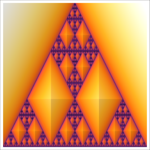
Figure 2: A two-dimensional “slice” of Han’s fractal $\delta^{*}$ in characteristic 3

We turn now to a couple of (related) examples with $n=4$.

Example 3.20.

Let $\Bbbk={\mathbb{F}}_{9}$, and $\epsilon\in\Bbbk$ with $\epsilon^{2}+2\epsilon+2=0$; let $\ell_{1},\ldots,\ell_{4}$ be $x$, $y$, $x+y$, and $x+\epsilon y$, and $C={\left({x,y}\right)}$. We examine the restriction of $\delta_{C}$ to the diagonal, namely the map ${\Delta_{1}}:\mathscr{I}\to\mathbb{Q}$, ${\Delta_{1}}(t)=\delta_{C}(t,t,t,t)$. The graph of ${\Delta_{1}}$ is shown in Figure 3.

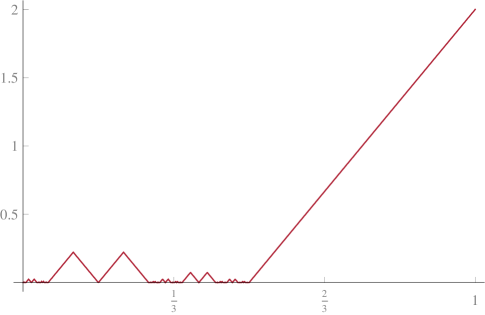
Figure 3: ${\Delta_{1}}(t)$ $(0\leq t\leq 1)$

The linear behavior on $[1/2,1]$ is expected from Remark 2.5: if $a/q\geq 1/2$ then $\deg(x^{a}y^{a}(x+y)^{a}(x+\epsilon y)^{a})\geq 2q$, so

$${\Delta_{1}}\left(\frac{a}{q}\right)=\frac{1}{q}\cdot\delta(x^{q},y^{q},x^{a}y^{a}(x+y)^{a}(x+\epsilon y)^{a})=\frac{1}{q}(4a-2q)=4\cdot\frac{a}{q}-2.$$

Note how the portion of the graph on the interval $[1/3,2/3]$ seems to be a miniature of the entire graph. A closer look at the portion over $[0,1/3]$ (Figure 4)

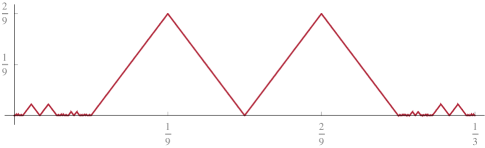
Figure 4: ${\Delta_{1}}(t)$ $(0\leq t\leq 1/3)$

shows small copies of the graph of ${\Delta_{1}}$ and its reflection about a vertical axis. These self-similarity properties will be investigated closely in a sequel to this paper.

The following property can also be inferred from the graphs: at any $t$, ${\Delta_{1}}(t)$ seems to be simply 4 times the distance from $t$ to the nearest zero of ${\Delta_{1}}$—so apparently ${\Delta_{1}}$ can be completely reconstructed from its zeros. This is in fact the case; see Section 4.

Example 3.21.

With $\Bbbk$, $\ell_{1},\ldots,\ell_{4}$, and $C$ as in the previous example, we now examine a two-dimensional “slice” of $\delta_{C}$, namely the map ${\Delta_{2}}:\mathscr{I}^{2}\to\mathbb{Q}$, ${\Delta_{2}}(t_{1},t_{2})=\delta_{C}(t_{1},t_{1},t_{2},t_{2})$. A relief plot of ${\Delta_{2}}$ is shown in Figure 5.

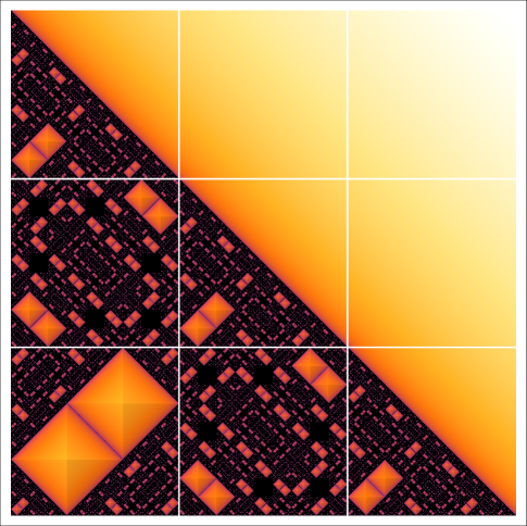
Figure 5: A two-dimensional “slice” of a 4-variable syzygy gap fractal

We immediately observe a simple behavior on a large portion of the domain: ${\Delta_{2}}$ is linear for $t_{1}+t_{2}\geq 1$, as expected from Remark 2.5. The grid dividing the plot into nine squares of equal size makes some self-similarity properties of ${\Delta_{2}}$ quite evident. (Figure 1 shows a magnification of one of those pieces—a two-dimensional “slice” of $\delta_{\left({x^{3},y^{3},xy}\right)}$, as will become clear after Section 5.3.) While in Section 5.3 we discuss a couple of these self-similarity properties, their thorough study will be left for a sequel to this paper, where we shall develop the tools to verify them rigorously.

Figure 6 shows some numerical values of the function

$$(i,j)\mapsto\frac{1}{2}\cdot\delta(x^{81},y^{81},x^{i}y^{i}(x+y)^{j}(x+\epsilon y)^{j})=\frac{81}{2}\cdot{\Delta_{2}}\left(\frac{i}{81},\frac{j}{81}\right),$$

where zeros are replaced by dots and the linear portion of the function is omitted.

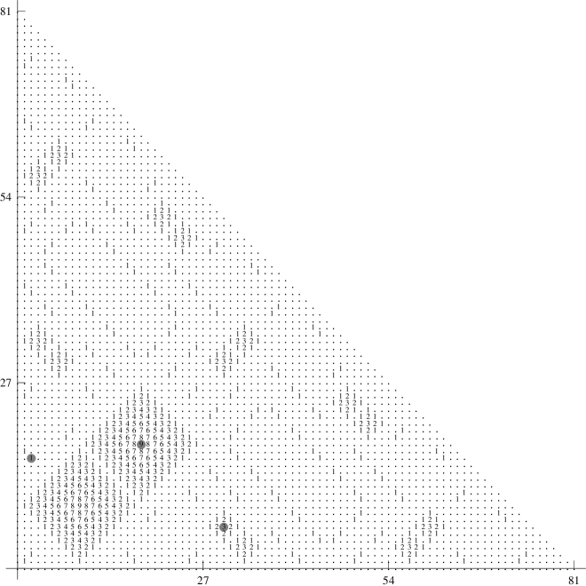
Figure 6: The function $(i,j)\mapsto\frac{1}{2}\cdot\delta(x^{81},y^{81},x^{i}y^{i}(x+y)^{j}(x+\epsilon y)^{j})$

From these numerical values we infer a property similar to that noticed in Example 3.20: at any point ${\mathbf{{t}}}$, ${\Delta_{2}}({\mathbf{{t}}})$ is simply twice the taxi-cab distance from ${\mathbf{{t}}}$ to the nearest zero of ${\Delta_{2}}$.

4 Syzygy gap fractals are determined by their zeros

Throughout this section we fix a cell $C$ with respect to pairwise prime linear forms $\ell_{1},\ldots,\ell_{n}$; we use results from Section 2 to prove that $\delta_{C}$, if nonlinear, is completely determined by its zeros, as suggested by the examples in the previous section. An important role is played by the Lipschitz property for $\delta_{C}$, which follows directly from Proposition 2.7:

Proposition 4.22.

For each ${\mathbf{{t}}}$ and ${\mathbf{{u}}}$ in $\mathscr{I}^{n}$ we have

$$|\delta_{C}({\mathbf{{t}}})-\delta_{C}({\mathbf{{u}}})|\leq d({\mathbf{{t}}},{\mathbf{{u}}}),$$

where $d({\mathbf{{t}}},{\mathbf{{u}}})$ is the taxi cab distance between ${\mathbf{{t}}}$ and ${\mathbf{{u}}}$, $d({\mathbf{{t}}},{\mathbf{{u}}})=\sum_{i=1}^{n}|t_{i}-u_{i}|.$

Remark 4.23.

A consequence of this is that we can extend (uniquely) $\delta_{C}$ to a continuous function $\delta^{*}_{C}:[0,1]^{n}\to\mathbb{R}$. The results of this section apply to $\delta^{*}_{C}$ as well, by continuity. This extension will be necessary in Section 6.

In what follows, ${\mathcal{X}}_{q}$ is the subset of $\mathscr{I}^{n}$ consisting of points that can be written as $(a_{1}/q,\ldots,a_{n}/q)$, with $a_{i}\in\mathbb{Z}$. In particular, ${\mathcal{X}}_{1}$ is simply $\{0,1\}^{n}$, the set of corners of $\mathscr{I}^{n}$.

Lemma 4.24.

Suppose $\delta_{C}|_{{\mathcal{X}}_{1}}$ attains a “local minimum” at a corner ${\mathbf{{u}}}$, in the sense that the values of $\delta_{C}$ at all corners adjacent to ${\mathbf{{u}}}$ are greater than $\delta_{C}({\mathbf{{u}}})$. Moreover, suppose $\delta_{C}({\mathbf{{u}}})>0$. Then

$$\delta_{C}({\mathbf{{t}}})=\delta_{C}({\mathbf{{u}}})+d({\mathbf{{t}}},{\mathbf{{u}}}),$$ (5)

for all ${\mathbf{{t}}}\in\mathscr{I}^{n}$. In particular $\delta_{C}$ is linear, everywhere positive, and has a minimum at ${\mathbf{{u}}}$ in the usual sense.

Proof 8.

In view of our local minimum assumption, Proposition 2.8 shows that $\delta_{C}({\mathbf{{v}}})=\delta_{C}({\mathbf{{u}}})+1$ for any corner ${\mathbf{{v}}}$ adjacent to ${\mathbf{{u}}}$. It follows from Proposition 4.22 that (5) holds for all points ${\mathbf{{t}}}$ along the edges containing ${\mathbf{{u}}}$.

Aiming at a contradiction, suppose that (5) fails for one or more points of ${\mathcal{X}}_{q}$. Among all such points, choose ${\mathbf{{t}}}$ whose distance to ${\mathbf{{u}}}$ is minimal. We know that ${\mathbf{{t}}}$ does not lie in any of the edges connecting to ${\mathbf{{u}}}$, so at least two coordinates of ${\mathbf{{t}}}$ and ${\mathbf{{u}}}$ must be different; say $u_{i}\neq t_{i}$ and $u_{j}\neq t_{j}$. Altering the $i$th or $j$th coordinates of ${\mathbf{{t}}}$ by $1/q$ we obtain points ${\mathbf{{v}}}$, ${\mathbf{{w}}}$, and ${\mathbf{{z}}}$ that are closer to ${\mathbf{{u}}}$, as illustrated in Figure 7.

Figure 7:

Let $s=\delta_{C}({\mathbf{{v}}})$; because of our choice of ${\mathbf{{t}}}$, we can use (5) to conclude that $\delta_{C}({\mathbf{{w}}})=s$ and $\delta_{C}({\mathbf{{z}}})=s-\frac{1}{q}$. But, since $\delta_{C}({\mathbf{{z}}})\geq\delta_{C}({\mathbf{{u}}})>0$, Proposition 2.10 then says that $\delta_{C}({\mathbf{{t}}})$ must equal $s+\frac{1}{q}$, and (5) holds for ${\mathbf{{t}}}$, contradicting our assumption. ∎

Theorem I.

Let ${\mathcal{Z}}=\{{\mathbf{{z}}}\in\mathscr{I}^{n}\,|\,\delta_{C}({\mathbf{{z}}})=0\}$.

• If ${\mathcal{Z}}$ is empty, then we are in the situation of Lemma 4.24, and $\delta_{C}$ is linear; it takes on a minimum value at a corner ${\mathbf{{u}}}$ of $\mathscr{I}^{n}$ and, at each ${\mathbf{{t}}}\in\mathscr{I}^{n}$,

  $$\delta_{C}({\mathbf{{t}}})=\delta_{C}({\mathbf{{u}}})+d({\mathbf{{t}}},{\mathbf{{u}}}).$$

• If ${\mathcal{Z}}$ is nonempty then $\delta_{C}({\mathbf{{t}}})$ is the taxi-cab distance from ${\mathbf{{t}}}$ to the set ${\mathcal{Z}}$, for all ${\mathbf{{t}}}\in\mathscr{I}^{n}$.

Proof 9.

If ${\mathcal{Z}}$ is empty, then there must be a corner ${\mathbf{{u}}}$ satisfying the hypothesis of the previous lemma. Suppose ${\mathcal{Z}}$ is nonempty. We shall show the result for ${\mathbf{{t}}}\in{\mathcal{X}}_{q}$, by induction on $\psi({\mathbf{{t}}})=q\cdot\delta_{C}({\mathbf{{t}}})$. If $\psi({\mathbf{{t}}})=0$, then ${\mathbf{{t}}}\in{\mathcal{Z}}$ and there is nothing to show, so suppose $\psi({\mathbf{{t}}})>0$. We claim that there is a ${\mathbf{{u}}}\in{\mathcal{X}}_{q}$ adjacent to ${\mathbf{{t}}}$ with $\psi({\mathbf{{u}}})<\psi({\mathbf{{t}}})$, so induction gives us the desired result.

To prove this claim, aiming at a contradiction suppose that $\delta_{C}({\mathbf{{u}}})>\delta_{C}({\mathbf{{t}}})>0$, for all ${\mathbf{{u}}}$ adjacent to ${\mathbf{{t}}}$ in ${\mathcal{X}}_{q}$. Then Proposition 2.9 shows that ${\mathbf{{t}}}$ must be a corner. If there were some adjacent corner ${\mathbf{{v}}}$ with $\delta_{C}({\mathbf{{v}}})<\delta_{C}({\mathbf{{t}}})$, then $\delta_{C}({\mathbf{{t}}})-\delta_{C}({\mathbf{{v}}})=1=d({\mathbf{{t}}},{\mathbf{{v}}})$, and Proposition 4.22 would show that $\delta_{C}$ is linear on the edge linking ${\mathbf{{t}}}$ and ${\mathbf{{v}}}$ (hence decreasing as one goes from ${\mathbf{{t}}}$ to ${\mathbf{{v}}}$); but that is not possible, as we are assuming that ${\mathbf{{t}}}$ is a local minimum in ${\mathcal{X}}_{q}$. This shows that ${\mathbf{{t}}}$ satisfies the hypothesis of Lemma 4.24. So $\delta_{C}$ is everywhere positive—but this contradicts our assumption that ${\mathcal{Z}}$ is nonempty. ∎

Theorem II.

Suppose $\delta_{C}|_{{\mathcal{X}}_{q}}$ attains a “local maximum” at ${\mathbf{{u}}}$, in the sense that the values of $\delta_{C}$ at all points of ${\mathcal{X}}_{q}$ adjacent to ${\mathbf{{u}}}$ are smaller than $\delta_{C}({\mathbf{{u}}})$. Then

$$\delta_{C}({\mathbf{{t}}})=\delta_{C}({\mathbf{{u}}})-d({\mathbf{{t}}},{\mathbf{{u}}}),$$ (6)

for all ${\mathbf{{t}}}\in\mathscr{I}^{n}$ with $d({\mathbf{{t}}},{\mathbf{{u}}})\leq\delta_{C}({\mathbf{{u}}})$. In particular, $\delta_{C}$ is piecewise linear on that region, and has a local maximum at ${\mathbf{{u}}}$ in the usual sense.

Proof 10.

We first prove the theorem for points of ${\mathcal{X}}_{q}$. If (6) is false for some ${\mathbf{{t}}}\in{\mathcal{X}}_{q}$ with $d({\mathbf{{t}}},{\mathbf{{u}}})\leq\delta_{C}({\mathbf{{u}}})$, choose one such ${\mathbf{{t}}}$ whose distance to ${\mathbf{{u}}}$ is minimal. If two or more coordinates of ${\mathbf{{t}}}$ and ${\mathbf{{u}}}$ are different, the argument used in Lemma 4.24 yields a contradiction; so suppose only the $i$th coordinates of ${\mathbf{{t}}}$ and ${\mathbf{{u}}}$ differ. Proposition 2.8 and the “local maximum” assumption show that ${\mathbf{{t}}}$ cannot be adjacent to ${\mathbf{{u}}}$ in ${\mathcal{X}}_{q}$. Modifying the $i$th coordinate of ${\mathbf{{t}}}$ by $1/q$ and $2/q$ we obtain points ${\mathbf{{v}}}$ and ${\mathbf{{w}}}$ closer to ${\mathbf{{u}}}$, as illustrated in Figure 8.

Figure 8:

Because of our choice of ${\mathbf{{t}}}$, Eq. (6) holds for these points, so $\delta_{C}({\mathbf{{w}}})>\delta_{C}({\mathbf{{v}}})>0$, and Proposition 2.9 shows that $\delta_{C}({\mathbf{{t}}})=\delta_{C}({\mathbf{{v}}})-1/q=\delta_{C}({\mathbf{{u}}})-d({\mathbf{{t}}},{\mathbf{{u}}})$, contradicting our assumption.

To complete the proof, note that since (6) holds for points adjacent to ${\mathbf{{u}}}$ in ${\mathcal{X}}_{q}$, it also holds on the edges connecting these adjacent points to ${\mathbf{{u}}}$, by Proposition 4.22. This shows that $\delta_{C}$ restricted to any ${\mathcal{X}}_{q^{\prime}}$ with $q^{\prime}\geq q$ also has a local maximum at ${\mathbf{{u}}}$; thus (6) holds for all ${\mathbf{{t}}}\in{\mathcal{X}}_{q^{\prime}}$ with $d({\mathbf{{t}}},{\mathbf{{u}}})\leq\delta_{C}({\mathbf{{u}}})$. ∎

5 Operators on cell classes

In this section we introduce a notion of equivalence of cells, and present a minimum on reflection and magnification operators on cell classes, to be used in Section 6. All cells here are with respect to an arbitrary fixed set of pairwise prime linear forms $\ell_{1},\ldots,\ell_{n}$, unless otherwise stated.

5.1 Cell classes

Definition 5.25.

Two cells $C_{1}$ and $C_{2}$ are $\delta$-equivalent if $\delta_{C_{1}}=\delta_{C_{2}}$. The equivalence class of a cell $C={\left({F,G,H}\right)}$ is denoted by $\mathscr{C}$ or ${\left[{F,G,H}\right]}$.

Remark 5.26.

Several properties follow immediately from the results from Sections 2 and 3:

1. Proposition 2.2: an equivalent cell results from any change in ${\left({F,G,H}\right)}$ that fixes the degrees of all the ideals ${\langle{F^{q},G^{q},H^{q}\ell^{\mathbf{{a}}}}\rangle}$ and the quantities $Q(\deg F^{q},\deg G^{q},\deg H^{q}\ell^{\mathbf{{a}}})$. In particular:

   • ${\left[{F,G,H}\right]}={\left[{G,F,H}\right]}$;

   • ${\left[{F,G,H}\right]}={\left[{aF,bG,cH}\right]}$, for nonzero $a,b,c\in\Bbbk$;

   • ${\left[{F,G,H}\right]}={\left[{F+UG+VH\ell,G,H}\right]}$ (and obvious variations), where $U$ and $V$ are homogeneous polynomials of appropriate degrees, provided $F+UG+VH\ell\neq 0$.

2. Proposition 3.14: ${\left[{F,G,H}\right]}={\left[{U,V}\right]}$, for some $U$ and $V$ such that ${\langle{U,V}\rangle}={\langle{F,G}\rangle}:H$.

3. Proposition 2.6: ${\left[{F,G,H}\right]}={\left[{PF,PG,H}\right]}$ (and obvious variations), for any nonzero homogeneous polynomial $P$ prime to $H\ell$.

Definition 5.27.

Let $\mathscr{C}$ be a cell class represented by a cell $C$. We define $\delta_{\mathscr{C}}=\delta_{C}$ and $\delta^{*}_{\mathscr{C}}=\delta^{*}_{C}$.

5.2 Reflections

Let $R_{1}:\mathscr{I}^{n}\to\mathscr{I}^{n}$ be the reflection in the first coordinate, i.e., the map that takes $(t_{1},t_{2},\ldots,t_{n})$ to $(1-t_{1},t_{2},\ldots,t_{n})$. Given a cell class $\mathscr{C}={\left[{F,G}\right]}$, we shall construct another cell class $R_{1}\mathscr{C}$ such that $\delta_{R_{1}\mathscr{C}}=\delta_{\mathscr{C}}\circ R_{1}$.

We may choose $F$ and $G$ of degree $\geq n$. Modifying one of these elements by a multiple of the other, we may assume that $F=\ell_{1}F^{*}$, for some $F^{*}$. Modifying $F$ by a multiple of $\ell$ we may assume that $\ell_{1}$ does not divide $F^{*}$. Since $\deg G\geq n$, $G$ is congruent to some $\ell_{1}G^{*}\pmod{\ell_{2}\cdots\ell_{n}}$, with $G^{*}\neq 0$. It is easy to see that $F^{*}$, $\ell_{1}G^{*}$, and $\ell$ have no common factor. Now let $R_{1}\mathscr{C}={\left[{F^{*},\ell_{1}G^{*}}\right]}.$

Proposition 5.28.

$\delta_{R_{1}\mathscr{C}}=\delta_{\mathscr{C}}\circ R_{1}$.

Proof 11.

By Proposition 2.6,

$$\delta_{\mathscr{C}}\left(\frac{{\mathbf{{a}}}}{q}\right)=\frac{1}{q}\cdot\delta\left(\ell_{1}^{q}{F^{*}}^{q},G^{q},\prod_{i=1}^{n}\ell_{i}^{a_{i}}\right)=\frac{1}{q}\cdot\delta\left(\ell_{1}^{q-a_{1}}{F^{*}}^{q},G^{q},\prod_{i=2}^{n}\ell_{i}^{a_{i}}\right).$$

Since $G^{q}-\ell_{1}^{q}{G^{*}}^{q}$ is a multiple of $\prod_{i=2}^{n}\ell_{i}^{a_{i}}$, by design, $G^{q}$ may be replaced with $\ell_{1}^{q}{G^{*}}^{q}$, and a couple more uses of Proposition 2.6 gives us

$$\delta_{\mathscr{C}}\left(\frac{{\mathbf{{a}}}}{q}\right) =\frac{1}{q}\cdot\delta\left(\ell_{1}^{q-a_{1}}{F^{*}}^{q},\ell_{1}^{q}{G^{*}}^{q},\prod_{i=2}^{n}\ell_{i}^{a_{i}}\right)$$

$$=\frac{1}{q}\cdot\delta\left({F^{*}}^{q},\ell_{1}^{a_{1}}{G^{*}}^{q},\prod_{i=2}^{n}\ell_{i}^{a_{i}}\right)$$

$$=\frac{1}{q}\cdot\delta\left({F^{*}}^{q},\ell_{1}^{q}{G^{*}}^{q},\ell_{1}^{q-a_{1}}\prod_{i=2}^{n}\ell_{i}^{a_{i}}\right)$$

$$=\delta_{R_{1}\mathscr{C}}\left(R_{1}\left(\frac{{\mathbf{{a}}}}{q}\right)\right).$$

∎

In particular, Proposition 5.28 shows that $\delta_{R_{1}\mathscr{C}}$ only depends on the cell class $\mathscr{C}$, and therefore the class $R_{1}\mathscr{C}$ is independent of the many choices made in its construction. So we have a well-defined operator $R_{1}$ on the set of cell classes. Furthermore, since $\delta_{R_{1}R_{1}\mathscr{C}}=\delta_{\mathscr{C}}\circ R_{1}\circ R_{1}=\delta_{\mathscr{C}}$, it follows that $R_{1}R_{1}\mathscr{C}=\mathscr{C}$, for any class $\mathscr{C}$, so $R_{1}$ is an involution on the set of cell classes. We may, of course, construct other reflection operators.

Definition 5.29.

Let $\mathscr{C}$ be a cell class and $1\leq i\leq n$. Choose a representative ${\left({\ell_{i}F^{*},G}\right)}$ for $\mathscr{C}$ where $\deg\ell_{i}F^{*},\deg G\geq n$ and $\ell_{i}$ does not divide $F^{*}$. Choose $G^{*}\neq 0$ such that $G\equiv\ell_{i}G^{*}\pmod{\ell/\ell_{i}}$. Then we define $R_{i}\mathscr{C}={\left[{F^{*},\ell_{i}G^{*}}\right]}.$ The $R_{i}$ are well-defined commuting involutions on the set of cell classes, and

$$\delta_{R_{i}\mathscr{C}}=\delta_{\mathscr{C}}\circ R_{i}.$$

We call the $R_{i}$ and their compositions reflection operators; if $R$ is a reflection operator we call $R\mathscr{C}$ a reflection of $\mathscr{C}$.

For later use, we prove that cell classes with a certain special property are unique up to reflection.

Definition 5.30.

Suppose $n\geq 3$. A cell class $\mathscr{C}$ is special if $\delta_{\mathscr{C}}=n-2$ at some corner ${\mathbf{{c}}}$ of $\mathscr{I}^{n}$, $\delta_{\mathscr{C}}=n-3$ at all corners adjacent to ${\mathbf{{c}}}$, and $\delta_{\mathscr{C}}=0$ at the corner opposite to ${\mathbf{{c}}}$.

The prototypical example of a special cell class is ${\left[{x,y}\right]}$. In fact, after a change of variables we may assume that $\ell_{1}=x$ and $\ell_{2}=y$, and it is then easy to see that $\delta_{\left[{x,y}\right]}({\mathbf{{1}}})=n-2$, where ${\mathbf{{1}}}=(1,\ldots,1)$, and $\delta_{\left[{x,y}\right]}=n-3$ at any corner adjacent to ${\mathbf{{1}}}$, while $\delta_{\left[{x,y}\right]}({\mathbf{{0}}})=\deg x-\deg y=0$.

Proposition 5.31.

Special cell classes are reflections of one another. In particular, each special cell class is a reflection of ${\left[{x,y}\right]}$.

Proof 12.

It suffices to show that there is only one special cell class $\mathscr{C}$ with $\delta_{\mathscr{C}}({\mathbf{{0}}})=n-2$; any other special cell class will necessarily be a reflection of $\mathscr{C}$. The cell class $\mathscr{C}$ may be represented by a cell ${\left({F,G}\right)}$ with $\deg F-\deg G=\delta_{\mathscr{C}}({\mathbf{{0}}})=n-2$. The assumption that $\delta_{\mathscr{C}}=n-3$ at all corners adjacent to ${\mathbf{{0}}}$ implies that $G$ is prime to each $\ell_{i}$, by Proposition 2.8. The assumption that $\delta_{\mathscr{C}}({\mathbf{{1}}})=0$ implies that $F\not\in{\langle{G,\ell}\rangle}$. (If $F=UG+V\ell$, with $U\neq 0$, then ${\left[{F,G}\right]}={\left[{UG,G}\right]}={\left[{U,1}\right]}$, and $\delta_{\mathscr{C}}({\mathbf{{1}}})=\delta(U,1,\ell)=2$; a similar contradiction is obtained if $U=0$.)

Since $F\not\in{\langle{G,\ell}\rangle}$, the polynomial $G$ is not constant, so $\deg F\geq n-1$. Thus the $\Bbbk$-vector space of elements of degree $\deg F$ in $\Bbbk[x,y]/{\langle{\ell}\rangle}$ is $n$-dimensional. A basis for that space consists of the elements represented by

$$F,\ x^{n-2}G,\ x^{n-3}yG,\ \ldots,\ y^{n-2}G,$$ (7)

which are linearly independent because $F\not\in{\langle{G,\ell}\rangle}$ and $G$ is prime to $\ell$.

Now suppose ${\left[{F_{1},G_{1}}\right]}$ is another cell class with the same properties. Remark 5.26(3) allows us to multiply ${\left({F,G}\right)}$ and ${\left({F_{1},G_{1}}\right)}$ by homogeneous polynomials prime to each $\ell_{i}$, so we may assume that $G_{1}=G$ and, a fortiori, $\deg F_{1}=\deg F$. So the image of $F_{1}$ in $\Bbbk[x,y]/{\langle{\ell}\rangle}$ can be written as a linear combination of the images of the elements in (7), and the third property in Remark 5.26(1) ensures that ${\left[{F_{1},G}\right]}={\left[{F,G}\right]}=\mathscr{C}$. ∎

Example 5.32.

For later use, let us find a representative for the special cell class $\mathscr{C}=R_{2}\cdots R_{n}{\left[{x,y}\right]}$. Changing variables, if necessary, we may assume that $\ell_{1}=x$ and $\ell_{2}=y$. Then

$$\delta_{\mathscr{C}}\left(\frac{{\mathbf{{a}}}}{q}\right) =\delta_{\left[{x,y}\right]}\left(R_{2}\cdots R_{n}\left(\frac{{\mathbf{{a}}}}{q}\right)\right)$$

$$=\frac{1}{q}\cdot\delta\left(x^{q},y^{q},x^{a_{1}}y^{q-a_{2}}\ell_{3}^{q-a_{3}}\cdots\ell_{n}^{q-a_{n}}\right).$$

Through repeated uses of Proposition 2.6 we find that

$$\delta\left(x^{q},y^{q},x^{a_{1}}y^{q-a_{2}}\ell_{3}^{q-a_{3}}\cdots\ell_{n}^{q-a_{n}}\right) =\delta\left(x^{q-a_{1}},y^{a_{2}},\ell_{3}^{q-a_{3}}\cdots\ell_{n}^{q-a_{n}}\right)$$

$$=\delta\left(x^{q},x^{a_{1}}y^{a_{2}}\ell_{3}^{a_{3}}\cdots\ell_{n}^{a_{n}},(\ell_{3}\cdots\ell_{n})^{q}\right),$$

so $\delta_{\mathscr{C}}({\mathbf{{a}}}/q)=\delta_{\left[{x,\ell_{3}\cdots\ell_{n}}\right]}({\mathbf{{a}}}/q)$, whence $\mathscr{C}={\left[{x,\ell_{3}\cdots\ell_{n}}\right]}$. But $\ell_{3}\cdots\ell_{n}\equiv cy^{n-2}\pmod{x}$, for some nonzero constant $c$, so we conclude that

$$R_{2}\cdots R_{n}{\left[{x,y}\right]}={\left[{x,y^{n-2}}\right]}.$$

Of course, in view of Proposition 5.31, the above identity could be just as easily verified by showing that ${\left[{x,y^{n-2}}\right]}$ is the special cell class with maximum at $(1,0,\ldots,0)$.

5.3 Magnification operators

Definition 5.33.

Let $q$ be a power of $p$ and ${\mathbf{{b}}}\in[q-1]^{n}$. Given $f:\mathscr{I}^{n}\to\mathbb{Q}$ we define $T_{q|{\mathbf{{b}}}}f:\mathscr{I}^{n}\to\mathbb{Q}$ as follows:

$$T_{q|{\mathbf{{b}}}}f({\mathbf{{t}}})=q\cdot f\left(\frac{{\mathbf{{t}}}+{\mathbf{{b}}}}{q}\right).$$

Remark 5.34.

This definition differs slightly from the one given in [8, 9].

We introduce operators on cell classes that are “compatible” with the action of the operators $T_{q|{\mathbf{{b}}}}$ on the functions $\delta_{\mathscr{C}}$.

Definition 5.35.

Let $\mathscr{C}={\left[{F,G,H}\right]}$. With notation as in Definition 5.33, we define $T_{q|{\mathbf{{b}}}}\mathscr{C}={\left[{F^{q},G^{q},H^{q}\ell^{{\mathbf{{b}}}}}\right]}.$ Then

$$\delta_{T_{q|{\mathbf{{b}}}}\mathscr{C}}=T_{q|{\mathbf{{b}}}}\delta_{\mathscr{C}},$$

so $T_{q|{\mathbf{{b}}}}\mathscr{C}$ does not depend on the choice of representative for $\mathscr{C}$. We call $T_{q|{\mathbf{{b}}}}$ a magnification operator and $T_{q|{\mathbf{{b}}}}\mathscr{C}$ a magnification of $\mathscr{C}$.

Example 5.36.

Suppose $\ell_{1}=x$ and $\ell_{2}=y$. Since ${\left[{x^{q},y^{q},x^{j}y^{k}}\right]}={\left[{x^{q-j},y^{q-k}}\right]}$, for $j,k\leq q$, we conclude that

$$T_{q|(j,k,0,\ldots,0)}{\left[{x,y}\right]}={\left[{x^{q-j},y^{q-k}}\right]}.$$ (8)

In particular, taking $q\geq n-2$ and setting $j=q-1$ and $k=q-n+2$ we find

$$T_{q|(q-1,q-n+2,0,\ldots,0)}{\left[{x,y}\right]}={\left[{x,y^{n-2}}\right]}=R_{2}\cdots R_{n}{\left[{x,y}\right]},$$

where the second equality comes from Example 5.32. This reveals an interesting self-similarity property of the syzygy gap fractal $\delta_{\left[{x,y}\right]}$:

$$T_{q|(q-1,q-n+2,0,\ldots,0)}\delta_{\left[{x,y}\right]}=\delta_{\left[{x,y}\right]}\circ R_{2}\cdots R_{n}.$$ (9)

Going back to (8) and setting $j=k=q-1$, we see that ${\left[{x,y}\right]}$ is fixed by the operator $T_{q|(q-1,q-1,0,\ldots,0)}$ and, consequently, so is $\delta_{\left[{x,y}\right]}$. The same holds, of course, for any $T_{q|{\mathbf{{b}}}}$ where ${\mathbf{{b}}}$ is a permutation of $(q-1,q-1,0,\ldots,0)$. This self-similarity property can be observed in Example 3.21—it explains why the NW and SE portions of the relief plot in Figure 5 are miniatures of the whole plot. The fact that the center portion is also a miniature of the whole plot is a consequence of the following result (of which the property discussed in this paragraph is a particular case, with $j=k=0$).

Proposition 5.37.

Suppose $n\geq 4$ and let ${\mathbf{{b}}}=(q-j-1,q-k-1,j,k,0,\ldots,0)$, for some $j,k<q$. Let $\lambda$ be the cross ratio of the roots in $\mathbb{P}^{1}(\Bbbk)$ of $\ell_{1}$, $\ell_{2}$, $\ell_{3}$, and $\ell_{4}$, and suppose $\alpha=\sum_{i=0}^{k}\binom{j}{k-i}\binom{k}{i}\lambda^{i}\neq 0$. Then ${\left[{x,y}\right]}$ is fixed by $T_{q|{\mathbf{{b}}}}$ (and consequently so is $\delta_{\left[{x,y}\right]}$). A similar result holds for any permutation of ${\mathbf{{b}}}$.

Proof 13.

A change of variables allows us to assume that $\ell_{1}=x$, $\ell_{2}=y$, $\ell_{3}=x+y$, and $\ell_{4}=x+\lambda y$. Then $\alpha$ is the coefficient of $x^{j}y^{k}$ in $(x+y)^{j}(x+\lambda y)^{k}$. By Proposition 2.6,

$$T_{q|{\mathbf{{b}}}}{\left[{x,y}\right]} ={\left[{x^{q},y^{q},x^{q-j-1}y^{q-k-1}(x+y)^{j}(x+\lambda y)^{k}}\right]}$$

$$={\left[{x^{j+1},y^{k+1},(x+y)^{j}(x+\lambda y)^{k}}\right]}.$$

All terms of $(x+y)^{j}(x+\lambda y)^{k}$ but $\alpha x^{j}y^{k}$ are multiples of $x^{j+1}$ or $y^{k+1}$, so $T_{q|{\mathbf{{b}}}}{\left[{x,y}\right]}={\left[{x^{j+1},y^{k+1},\alpha x^{j}y^{k}}\right]}={\left[{x,y,\alpha}\right]}={\left[{x,y}\right]}$. ∎

When $j=k=1$ the condition on $\alpha$ in the above proposition is simply that $\lambda\neq-1$. This is the case in Example 3.21, and explains why the center portion of the relief plot shown in Figure 5 is a miniature of whole plot.

We end this section with a proof that the $\delta_{\mathscr{C}}$ are $p$-fractals when the field $\Bbbk$ is finite. We recall the definition of $p$-fractal first:

Definition 5.38.

A function $f:\mathscr{I}^{n}\to\mathbb{Q}$ is a $p$-fractal if the $\mathbb{Q}$-vector space spanned by $f$ and all the magnifications $T_{q|{\mathbf{{b}}}}f$ is finite dimensional.

Theorem 5.39.

If the field $\Bbbk$ is finite, then there are only finitely many nonlinear $\delta_{\mathscr{C}}$. In particular, the $\delta_{\mathscr{C}}$ are $p$-fractals.

Proof 14.

We start by showing that every cell class has a representative ${\left({F,G}\right)}$ with $\deg F\leq n$. In fact, suppose $\mathscr{C}={\left[{F,G}\right]}$, with $\deg F$ and $\deg G$ greater than $n$. Take $U$ of degree $\leq 2$ and prime to $\ell$; it is easy to see that ${\langle{F,G}\rangle}\subseteq{\langle{x,y}\rangle}^{\deg U+n-1}\subseteq{\langle{U,\ell}\rangle}$, so by modifying $F$ and $G$ by multiples of $\ell$ we may assume that both are multiples of $U$. Since $U$ is prime to $\ell$ we can also divide $F$ and $G$ by $U$ without affecting $\mathscr{C}$, obtaining a new representative consisting of polynomials of smaller degrees.

Now note that if $\deg G-\deg F\geq n$, Proposition 2.6 and Remark 2.5 show that $\delta_{\mathscr{C}}$ is linear. Together with the result from the previous paragraph, this shows that any cell class $\mathscr{C}$ with nonlinear $\delta_{\mathscr{C}}$ can be represented by a cell ${\left({F,G}\right)}$ with $\deg F\leq n$ and $\deg G-\deg F<n$. If $\Bbbk$ is finite, there are only finitely many such cells.

The conclusion that the $\delta_{\mathscr{C}}$ are $p$-fractals follows at once, since the $\mathbb{Q}$-vector space spanned by the finitely many nonlinear $\delta_{\mathscr{C}}$, the constant function 1, and the coordinate functions is stable under the operators $T_{q|{\mathbf{{b}}}}$. ∎

6 An upper bound

Throughout this section we fix pairwise prime linear forms $\ell_{1},\ldots,\ell_{n}$ in $\Bbbk[x,y]$. Cells and cell classes are defined with respect to these linear forms, unless otherwise stated.

In [7, Theorem 8] Monsky found an upper bound for the local maxima of the $\delta_{\mathscr{C}}$: if $\delta_{\mathscr{C}}=\delta_{\left[{F,G,H}\right]}$ has a local maximum at ${\mathbf{{a}}}/q$, where $q>1$ and some $a_{i}$ is not divisible by $p$, then

$$\delta_{\mathscr{C}}\left(\frac{{\mathbf{{a}}}}{q}\right)\leq\frac{n_{0}-2}{q},$$

where $n_{0}$ is the number of zeros of $FGH\ell$ in $\mathbb{P}^{1}\left(\bar{\Bbbk}\right)$ (not counted with multiplicity).

Example 6.40.

In Examples 3.20 and 3.21 we looked at “slices” of a syzygy gap fractal $\delta_{\mathscr{C}}:\mathscr{I}^{4}\to\mathbb{Q}$; Figure 6 shows some related numerical values. From the three points highlighted in that picture we can gather (with the help of Theorem II) that $\delta_{\mathscr{C}}$ has local maxima at the points $(2,2,2,2)/9$, $(10,10,2,2)/27$, and $(2,2,16,16)/81$, where it takes on the values $2/9$, $2/27$, and $2/81$, respectively. Since here $n_{0}=4$, Monsky’s bound is attained in each case.

In this section we sharpen Monsky’s result, proving the following:

Theorem III.

Suppose $\delta_{\mathscr{C}}$ has a local maximum at ${\mathbf{{a}}}/q$, where $q>1$ and ${\mathbf{{a}}}/q$ is reduced, in the sense that some coordinate $a_{i}/q$ is reduced. Then

$$\delta_{\mathscr{C}}\left(\frac{{\mathbf{{a}}}}{q}\right)\leq\frac{n-2}{q}.$$

Remark 6.41.

If $\mathscr{C}$ is a special cell class (see Definition 5.30), this is nothing but Monsky’s bound, since in view of Proposition 5.31 we may assume that $\mathscr{C}={\left[{x,y}\right]}={\left[{\ell_{1},\ell_{2}}\right]}$, whence $n_{0}=n$.

The approach used in our proof was suggested by Monsky, and follows closely an alternate proof he provided of his result from [7] (private communication). Before we dive into the proof of the theorem, we look at a couple of consequences.

Corollary 6.42.

Let $q>1$, and fix $(a_{2},\ldots,a_{n})\in[q]^{n-1}$. Suppose the map

$$t\mapsto\delta_{\mathscr{C}}(t,a_{2}/q,\ldots,a_{n}/q)$$

has a local maximum at $a_{1}/q$, where $a_{1}$ is not divisible by $p$, and let ${\mathbf{{a}}}=(a_{1},a_{2},\ldots,a_{n})$. Then

$$\delta_{\mathscr{C}}\left(\frac{{\mathbf{{a}}}}{q}\right)\leq\frac{n-2}{q}.$$

Proof 15.

According to Theorem II, each local maximum ${\mathbf{{u}}}$ of $\delta_{\mathscr{C}}|_{{\mathcal{X}}_{q}}$ determines a region on which $\delta_{\mathscr{C}}$ is piecewise linear, given by $\delta_{\mathscr{C}}({\mathbf{{t}}})=\delta_{\mathscr{C}}({\mathbf{{u}}})-d({\mathbf{{t}}},{\mathbf{{u}}})$. The point ${\mathbf{{a}}}/q$ is in one such region, and because the map $t\mapsto\delta_{\mathscr{C}}(t,a_{2}/q,\ldots,a_{n}/q)$ has a local maximum at $a_{1}/q$, it must be the case that $u_{1}=a_{1}/q$. So ${\mathbf{{u}}}$ satisfies the assumptions of Theorem III, and $\delta_{\mathscr{C}}\left({\mathbf{{a}}}/q\right)\leq\delta_{\mathscr{C}}\left({\mathbf{{u}}}\right)\leq(n-2)/q.$ ∎

The next corollary provides an answer to a question raised in [8, Section 7(4)] in a special case.

Corollary 6.43.

Let $C={\left({F,G,H}\right)}$ be a cell, and ${\mathbf{{a}}}=(a_{1},\ldots,a_{n})\in[q]^{n}$ with $a_{1}$ not divisible by $p$. Then

$$2\deg{\langle{F^{q},G^{q},H^{q}\ell^{\mathbf{{a}}}}\rangle}-\deg{\langle{F^{q},G^{q},H^{q}\ell^{\mathbf{{a}}}\ell_{1}}\rangle}-\deg{\langle{F^{q},G^{q},H^{q}\ell^{\mathbf{{a}}}/\ell_{1}}\rangle}\leq n-2.$$ (10)

Proof 16.

Let $\delta$, $\delta_{+}$, and $\delta_{-}$ denote the syzygy gaps correspondent to the degrees on the left hand side of (10), namely $\delta(F^{q},G^{q},H^{q}\ell^{\mathbf{{a}}})$, $\delta(F^{q},G^{q},H^{q}\ell^{\mathbf{{a}}}\ell_{1})$, and $\delta(F^{q},G^{q},H^{q}\ell^{\mathbf{{a}}}/\ell_{1})$. Proposition 2.2 transforms (10) into

$$\frac{1}{4}(2+2\delta^{2}-\delta_{+}^{2}-\delta_{-}^{2})\leq n-2.$$

If $\delta_{-}=\delta-1$ and $\delta_{+}=\delta+1$ (or vice-versa), then $2+2\delta^{2}-\delta_{+}^{2}-\delta_{-}^{2}=0$. If $\delta_{\pm}=\delta+1$, then $\delta=0$, by Proposition 2.9, so again $2+2\delta^{2}-\delta_{+}^{2}-\delta_{-}^{2}=0$. Finally, if $\delta_{\pm}=\delta-1$, then $(2+2\delta^{2}-\delta_{+}^{2}-\delta_{-}^{2})/4=\delta$. But in this situation the map $t\mapsto\delta_{\mathscr{C}}(t,a_{2}/q,\ldots,a_{n}/q)$ has a local maximum at $a_{1}/q$, and Corollary 6.42 shows that $\delta\leq n-2$. ∎

In the remainder of this section we fix a cell class $\mathscr{C}={\left[{U,V}\right]}$. In view of Remark 5.26(3) we may assume that $U$ and $V$ have no common factor. Since the values of our functions remain unchanged if we extend $\Bbbk$, we may also assume without loss of generality that $\Bbbk$ is algebraically closed.

6.1 Some reductions, a special case, and a proof outline

• (We may assume $q=p$.) In the situation of the statement of Theorem III, write ${\mathbf{{a}}}=p\cdot{\mathbf{{b}}}+{\mathbf{{c}}}$, with $0\leq c_{i}<p$, and let $q^{\prime}=q/p$. Then

  $$\delta_{\mathscr{C}}\left(\frac{{\mathbf{{a}}}}{q}\right)=\delta_{\mathscr{C}}\left(\frac{{\mathbf{{c}}}/p+{\mathbf{{b}}}}{q^{\prime}}\right)=\frac{1}{q^{\prime}}\cdot(T_{q^{\prime}|{\mathbf{{b}}}}\delta_{\mathscr{C}})\left(\frac{{\mathbf{{c}}}}{p}\right)=\frac{1}{q^{\prime}}\cdot\delta_{T_{q^{\prime}|{\mathbf{{b}}}}\mathscr{C}}\left(\frac{{\mathbf{{c}}}}{p}\right),$$

  and $\delta_{T_{q^{\prime}|{\mathbf{{b}}}}\mathscr{C}}$ has a local maximum at ${\mathbf{{c}}}/p$. Moreover, since ${\mathbf{{a}}}/q$ is reduced, so is ${\mathbf{{c}}}/p$. The above equation also shows that $\delta_{\mathscr{C}}({\mathbf{{a}}}/q)\leq(n-2)/q$ whenever $\delta_{T_{q^{\prime}|{\mathbf{{b}}}}\mathscr{C}}({\mathbf{{c}}}/p)\leq(n-2)/p$. So it suffices to prove Theorem III for $q=p$.

• (The trivial cases $n=1,2$.) Theorem III is vacuously true when $n=1$ or 2, since in those cases the $\delta_{\mathscr{C}}$, completely described in Example 3.17, only have local maxima at the endpoints of $\mathscr{I}$ or corners of $\mathscr{I}^{2}$.

• (Focusing on interior points.) Note that each restriction of $\delta_{\mathscr{C}}$ to a face of $\mathscr{I}^{n}$ agrees with the values of a function $\delta_{\mathscr{C}^{\prime}}:\mathscr{I}^{n-1}\to\mathbb{Q}$. Indeed, for $\epsilon=0$ or 1, $\delta_{\mathscr{C}}(u_{1},\ldots,u_{n-1},\epsilon)=\delta_{\mathscr{C}^{\prime}}(u_{1},\ldots,u_{n-1})$, where $\mathscr{C^{\prime}}={\left[{U,V,\ell_{n}^{\epsilon}}\right]}$, a cell class defined with respect to the linear forms $\ell_{1},\ldots,\ell_{n-1}$. So induction on $n$ will allow us to restrict our attention to interior points of $\mathscr{I}^{n}$.

These simple remarks allow us to prove Theorem III for $p=2$.

Proof of Theorem III (for $p=2$) 1.

The theorem holds for $n=1$ and 2, so we let $n>2$ and argue by induction on $n$. As shown above, it suffices to consider the case $q=p=2$. Suppose $\delta_{\mathscr{C}}$ has a local maximum at ${\mathbf{{t}}}={\mathbf{{a}}}/2$, where ${\mathbf{{a}}}\in[2]^{n}$, with some $a_{i}=1$. If ${\mathbf{{t}}}$ lies in a face of $\mathscr{I}^{n}$, the observation made above and the induction hypothesis give us the desired bound. It remains to consider ${\mathbf{{a}}}=(1,\ldots,1)$. Aiming at a contradiction, we suppose $\delta_{\mathscr{C}}({\mathbf{{t}}})>(n-2)/2$. Theorem II shows that $(1/2,\ldots,1/2,0)$ is a local maximum of the restriction of $\delta_{\mathscr{C}}$ to that face of $\mathscr{I}^{n}$. The induction hypothesis then gives $\delta_{\mathscr{C}}(1/2,\ldots,1/2,0)\leq(n-3)/2$, and it follows that $\delta_{\mathscr{C}}({\mathbf{{t}}})\leq(n-2)/2$, a contradiction. ∎

In view of the above, from now on we assume that $p\neq 2$ and $n>2$. Our proof will consist of four steps.

Proof outline:

1. In Section 6.2 we relate $\delta^{*}_{\mathscr{C}}({\mathbf{{c}}}/m)$, where $m<\sum_{i=1}^{n}c_{i}$, to the Hilbert–Kunz multiplicity of a 3-variable homogeneous polynomial $F=\ell^{{\mathbf{{c}}}}-z^{m}H$ with respect to the ideal ${\langle{U,V,z}\rangle}$, under the assumption that $\deg U=\deg V$ (or, equivalently, $\delta_{\mathscr{C}}({\mathbf{{0}}})=0$).

2. In Section 6.3 we use results of Brenner and Trivedi to find another formula for that Hilbert–Kunz multiplicity, thereby obtaining some information on $\delta^{*}_{\mathscr{C}}({\mathbf{{c}}}/m)$.

3. In Section 6.4 we prove that if $\delta_{\mathscr{C}}$ has a local maximum at a point ${\mathbf{{a}}}/q$, where $\delta_{\mathscr{C}}({\mathbf{{0}}})=0$, $\delta_{\mathscr{C}}({\mathbf{{a}}}/q)\geq(n-1)/q$, and $d({\mathbf{{a}}}/q,{\mathbf{{0}}})>1$, then $\sum_{i=1}^{n}a_{i}\equiv 0\pmod{p}$. That is done by choosing a convenient point ${\mathbf{{c}}}/m$, close enough to ${\mathbf{{a}}}/q$ to be “under the effect” of that local maximum, and using the information on $\delta^{*}_{\mathscr{C}}({\mathbf{{c}}}/m)$ previously found. Reflections then show that each corner ${\mathbf{{b}}}$ with $\delta_{\mathscr{C}}({\mathbf{{b}}})=0$ and $d({\mathbf{{a}}}/q,{\mathbf{{b}}})>1$ yields a congruence of the form $\sum_{i=1}^{n}(\pm a_{i})\equiv 0\pmod{p}$.

4. We conclude the proof in Section 6.5: assuming that $\delta_{\mathscr{C}}$ has a local maximum at an interior point ${\mathbf{{a}}}/p$, where it takes on a value $\geq(n-1)/p$, we shall show that there are enough corners ${\mathbf{{b}}}$ as above, with $\delta_{\mathscr{C}}({\mathbf{{b}}})=0$ and $d({\mathbf{{a}}}/p,{\mathbf{{b}}})>1$, to guarantee that the corresponding congruences lead to a contradiction. Special cell classes are handled separately, through a simpler argument that takes advantage of their self-similarities.

6.2 Hilbert–Kunz multiplicities and syzygy gaps

Recall that $\mathscr{C}={\left[{U,V}\right]}$, where $U$ and $V$ have no common factor; in this subsection we add the extra assumption that $\deg U=\deg V=d$. We denote by $\delta^{*}_{\mathscr{C}}$ the continuous extension of $\delta_{\mathscr{C}}$ to $[0,1]^{n}$, as in Remark 4.23.

Let ${\mathbf{{c}}}$ be a nonnegative integer vector, $G=\ell^{\mathbf{{c}}}$, and $r=\deg G$. Fix $m$ with $0<m<r$ such that ${\mathbf{{c}}}/m\in[0,1]^{n}$. Let $H\in\Bbbk[x,y]$ be a homogeneous polynomial of degree $r-m$, prime to $G$, and set $F=G-z^{m}H\in\Bbbk[x,y,z]$.

Definition 6.44.

$\mu(F)$ is the Hilbert–Kunz multiplicity of $\Bbbk[x,y,z]/{\langle{F}\rangle}$ with respect to the ideal generated by the images of $U$, $V$, and $z$.

We shall relate $\mu(F)$ and $\delta^{*}_{\mathscr{C}}({\mathbf{{c}}}/m)$, proving:

Theorem 6.45.

$\displaystyle\mu(F)=dr-\frac{r}{4}+\frac{m^{2}}{4r}\cdot\delta_{\mathscr{C}}^{*}\left(\frac{{\mathbf{{c}}}}{m}\right)^{2}.$

Lemma 6.46.

Let $\lambda=\lambda(F)$ be the greatest divisor of $m$ for which $G/H$ is a $\lambda$th power in $\Bbbk(x,y)$. Then:

1. If $\lambda=1$, then $F$ is irreducible in $\Bbbk[x,y,z]$.

2. If Theorem 6.45 holds for $\lambda=1$, then it holds in general.

Proof 17.

Since $G$ and $H$ are relatively prime, any nontrivial factorization of $F=G-z^{m}H$ in $\Bbbk[x,y,z]$ would have factors of degree $<m$ in $z$, giving a nontrivial factorization of $z^{m}-G/H$ in $\Bbbk(x,y)[z]$. But $z^{m}-G/H$ is irreducible in $\Bbbk(x,y)[z]$ if $\lambda=1$ (see, e.g., [5, Chapter VI, Theorem 9.1]); this gives us 1.

Suppose now $\lambda>1$. Since $G$ and $H$ are relatively prime, both $G$ and $H$ are $\lambda$th powers, and we can write $z^{\lambda}-G/H=\prod_{i=1}^{\lambda}(z-\ell^{{\mathbf{{c}}}/\lambda}/H_{i})$, where the $H_{i}$ are $\lambda$th roots of $H$. Replacing $z$ with $z^{m/\lambda}$ and multiplying through by $H$ we see that $F=F_{1}\cdots F_{\lambda}$, where $F_{i}=\ell^{{\mathbf{{c}}}/\lambda}-z^{m/\lambda}H_{i}$. If Theorem 6.45 holds for $\lambda=1$, it gives formulas for the Hilbert–Kunz multiplicity $\mu(F_{i})$ of each $F_{i}$. But the additivity of the Hilbert–Kunz multiplicity shows that $\mu(F)=\sum_{i=1}^{\lambda}\mu(F_{i})$, and adding up those formulas gives Theorem 6.45 for $F$. ∎

In the remainder of this section we assume that $\lambda(F)=1$, so $F$ is irreducible in $\Bbbk[x,y,z]$. Let $\bar{z}$ and $w$ be elements in an extension of $\Bbbk(x,y)$ such that $\bar{z}^{m}=G$ and $w^{m}=H$. Set $\bar{x}=wx$ and $\bar{y}=wy$. Then

$$F(\bar{x},\bar{y},\bar{z}) =G(\bar{x},\bar{y})-\bar{z}^{m}H(\bar{x},\bar{y})$$

$$=w^{r}G(x,y)-G(x,y)\cdot w^{r-m}H(x,y)$$

$$=w^{r}G(x,y)-G(x,y)\cdot w^{r-m}\cdot w^{m}$$

$$=0,$$

so $\Bbbk[\bar{x},\bar{y},\bar{z}]$ is a homogeneous coordinate ring for $F$. We now consider the rings in the following diagram.

Here $\alpha$ and $\beta$ denote the ranks of $A$ and $B$ over $R$; these are finite, according to the next lemma.

Lemma 6.47.

$A$ and $B$ are finite over $R$.

Proof 18.

The ideal ${\langle{H^{d}U^{m},H^{d}V^{m},G}\rangle}$ of $A$ is ${\langle{x,y}\rangle}$-primary, as its generators have no common factor; so it contains $x^{s}$ and $y^{s}$ for some $s$. Let $M$ be the $R$-submodule of $A$ generated by $x^{i}y^{j}$, with $i+j\leq 2s-2$. Writing $x^{s}$ and $y^{s}$ as $A$-linear combinations of $H^{d}U^{m}$, $H^{d}V^{m}$, and $G$, we see that they can be expressed as $R$-linear combinations of monomials of degree $<s$. It follows easily that $xM\subseteq M$ and $yM\subseteq M$, so that any monomial in $x$ and $y$ is in $M$. Hence $A=M$, and $A$ is finite over $R$.

Arguing along the same lines, choosing $s$ such that $x^{s}$ and $y^{s}$ are in the ideal ${\langle{U^{m},V^{m}}\rangle}$ of $A$ we can show that $B$ is generated over $R$ by monomials $\bar{x}^{i}\bar{y}^{j}\bar{z}^{k}$, with $i+j\leq 2s-2$ and $k<m$. ∎

Definition 6.48.

For any nonnegative integer $k$, $\mu(k)$ is the Hilbert–Kunz multiplicity of $B$ with respect to the ideal $J(k)={\langle{U(\bar{x},\bar{y})^{k},V(\bar{x},\bar{y})^{k},\bar{z}^{k}}\rangle}$.

Lemma 6.49.

$\mu(km)=(\beta/\alpha)\cdot\deg J$, where $J$ is the ideal of $A$ generated by $H^{kd}U^{km}$, $H^{kd}V^{km}$, and $G^{k}$.

Proof 19.

The generators of $J$ are precisely the generators of $J(km)$, and are elements of $R$; let $I$ be the ideal they generate in $R$. Then $\mu(km)$ coincides with the Hilbert–Kunz multiplicity of $B$ (seen as an $R$-module) with respect to $I$. Using Theorem 1.8 of [6] we see that this Hilbert–Kunz multiplicity is just $\beta/\alpha$ times the Hilbert–Kunz multiplicity of $A$ with respect to $I$. But this is $(\beta/\alpha)\cdot\deg IA$, since $A=\Bbbk[x,y].$ ∎

Lemma 6.50.

$\beta/\alpha=m^{2}/r$.

Proof 20.

Let

$$K=\Bbbk\left(\frac{U(\bar{x},\bar{y})^{m}}{V(\bar{x},\bar{y})^{m}},\frac{V(\bar{x},\bar{y})^{m}}{\bar{z}^{dm}}\right)=\Bbbk\left(\frac{U^{m}}{V^{m}},\frac{H^{d}V^{m}}{G^{d}}\right)\subseteq\Bbbk\left(\frac{x}{y}\right)=\Bbbk\left(\frac{\bar{x}}{\bar{y}}\right).$$

The field of fractions of $R$ is $K(G)=K(\bar{z}^{m})$, and $\alpha$ and $\beta$ are the degrees of $\Bbbk(x,y)$ and $\Bbbk(\bar{x},\bar{y},\bar{z})$ over that field. Because $\bar{z}$ is a root of the degree $m$ irreducible polynomial $F(\bar{x},\bar{y},z)\in\Bbbk(\bar{x},\bar{y})[z]$ (see the proof of Lemma 6.46), we have

$$\beta =\left[\Bbbk\left(\bar{x},\bar{y},\bar{z}\right):\Bbbk\left(\bar{x},\bar{y}\right)\right]\cdot\left[\Bbbk\left(\bar{x},\bar{y}\right):\Bbbk\left(\bar{x}/\bar{y},\bar{y}^{m}\right)\right]\cdot\left[\Bbbk\left(\bar{x}/\bar{y},\bar{y}^{m}\right):K\left(G\right)\right]$$

$$=m^{2}\cdot\left[\Bbbk\left(\bar{x}/\bar{y},\bar{y}^{m}\right):K\left(G\right)\right].$$

But $\bar{y}^{m}/G=w^{m}y^{m}/G=Hy^{m}/G\in\Bbbk(x/y)=\Bbbk(\bar{x}/\bar{y})$, so $\Bbbk(\bar{x}/\bar{y},\bar{y}^{m})=\Bbbk(x/y,G)$, and

$$\beta=m^{2}\cdot\left[\Bbbk\left(x/y,G\right):K(G)\right].$$ (11)

A similar calculation gives

$$\alpha =\left[\Bbbk(x,y):\Bbbk\left(x/y,y^{r}\right)\right]\cdot\left[\Bbbk\left(x/y,y^{r}\right):K(G)\right]$$

$$=r\cdot\left[\Bbbk\left(x/y,G\right):K(G)\right],$$ (12)

and comparing (11) and (20) we get the desired result. ∎

Corollary 6.51.

$\displaystyle\mu(km)=k^{2}m^{2}dr-\frac{k^{2}m^{2}r}{4}+\frac{m^{2}}{4r}\cdot\delta(U^{km},V^{km},G^{k})^{2}.$

Proof 21.

Note that $Q(kdr,kdr,kr)=4dk^{2}r^{2}-k^{2}r^{2}$, where $Q$ is the quadratic form of Proposition 2.2. So Lemmas 6.49 and 6.50, together with Proposition 2.2, give us

$$\mu(km)=\frac{m^{2}}{4r}\left(4dk^{2}r^{2}-k^{2}r^{2}+\delta(H^{kd}U^{km},H^{kd}V^{km},G^{k})^{2}\right).$$

But $\delta(H^{kd}U^{km},H^{kd}V^{km},G^{k})=\delta(U^{km},V^{km},G^{k})$, by Proposition 2.6. ∎

We now need a “continuous version” of the above result; we shall arrive at the desired formula for $\mu(F)$ by replacing $k$ with $1/m$ in that continuous version.

Definition 6.52.

$\delta_{G}^{*}:[0,1]^{3}\to\mathbb{R}$ is the continuous function such that

$$\delta_{G}^{*}\left(\frac{{\mathbf{{a}}}}{q}\right)=\frac{1}{q}\cdot\delta(U^{a_{1}},V^{a_{2}},G^{a_{3}}),$$

for any $q$ and any ${\mathbf{{a}}}\in[q]^{3}$.

Directly from the definition of Hilbert–Kunz multiplicity it follows that $\mu(pk)=p^{2}\cdot\mu(k)$, so we may define a function $\mathscr{I}\to\mathbb{Q}$, $k/q\mapsto q^{-2}\cdot\mu(k)$. This function is uniformly continuous (see A for a proof in a more general setting), so we can extend it to a continuous function on $[0,1]$.

Definition 6.53.

$\mu^{*}:[0,1]\to\mathbb{R}$ is the continuous extension of the function $k/q\mapsto q^{-2}\cdot\mu(k)$.

Corollary 6.54.

$\displaystyle\mu^{*}(tm)=t^{2}m^{2}dr-\frac{t^{2}m^{2}r}{4}+\frac{m^{2}}{4r}\cdot\delta_{G}^{*}(tm,tm,t)^{2}$, for all $t\in[0,1/m].$

Proof 22.

Corollary 6.51 gives the formula for $t\in[0,1/m]\cap\mathbb{Z}[1/p]$, and the result follows by continuity. ∎

We can now complete the proof of Theorem 6.45.

Proof of Theorem 6.45 1.

Since, for any $q$ and $a\in[q]$,

$$\delta_{G}^{*}\left(1,1,\frac{a}{q}\right) =\frac{1}{q}\cdot\delta(U^{q},V^{q},G^{a})$$

$$=\frac{1}{q}\cdot\delta(U^{q},V^{q},\ell^{a{\mathbf{{c}}}})$$

$$=\delta_{\mathscr{C}}^{*}\left(\frac{a}{q}\cdot{\mathbf{{c}}}\right),$$

the continuity of $\delta_{G}^{*}$ and $\delta_{\mathscr{C}}^{*}$ implies that $\delta_{G}^{*}(1,1,t)=\delta_{\mathscr{C}}^{*}(t{\mathbf{{c}}})$, for any $t\in[0,1]$. Setting $t=1/m$ in the identity of Corollary 6.54 we get the desired result:

$$\mu(F)=\mu(1)=dr-\frac{r}{4}+\frac{m^{2}}{4r}\cdot\delta_{G}^{*}\left(1,1,\frac{1}{m}\right)^{2}=dr-\frac{r}{4}+\frac{m^{2}}{4r}\cdot\delta_{\mathscr{C}}^{*}\left(\frac{{\mathbf{{c}}}}{m}\right)^{2}.$$

∎

6.3 An application of sheaf theory

Definition 6.55.

Let $F\in\Bbbk[x,y,z]$ be an irreducible homogeneous polynomial, and ${Y}$ be a desingularization of the projective curve defined by $F$. Then $\gamma(F)=2\operatorname{genus}({Y})-2$.

The following result will be essential to our argument:

Theorem 6.56.

Let $q>1$ be a power of $p$. Let $F\in\Bbbk[x,y,z]$ be an irreducible degree $r$ homogeneous polynomial, and let $\mu(F)$ be the Hilbert–Kunz multiplicity of $\Bbbk[x,y,z]/{\langle{F}\rangle}$ with respect to a zero-dimensional ideal $I$ generated by three homogeneous elements of degrees $d_{1}$, $d_{2}$, and $d_{3}$. Then

$$\mu(F)=\frac{r}{4}\cdot Q(d_{1},d_{2},d_{3})+\frac{l^{2}}{4r},$$ (13)

where $l$ is a number in $\mathbb{Z}[1/p]$ such that $ql\in p\mathbb{Z}$ or $0<ql\leq\gamma(F)$, and $Q$ is the quadratic form of Proposition 2.2,

$$Q(d_{1},d_{2},d_{3})=2d_{1}d_{2}+2d_{1}d_{3}+2d_{2}d_{3}-{d_{1}}^{2}-{d_{2}}^{2}-{d_{3}}^{2}.$$

When $d_{1}=d_{2}=d_{3}=1$ this is Theorem 5.3 of Trivedi [11]. The general case is treated similarly, but now we need a result from Brenner [1] and a lemma of Trivedi. Before we give the proof, we recall some of the terminology used in those papers. For a rank $r$ vector bundle ${\mathcal{S}}$ on a smooth projective curve ${Y}$ over an algebraically closed field, $\deg({\mathcal{S}})$ is the degree of the line bundle $\bigwedge^{r}{\mathcal{S}}$; the degree is additive in the category of vector bundles on ${Y}$. The slope of ${\mathcal{S}}$ is defined as $\deg({\mathcal{S}})/r$. The vector bundle ${\mathcal{S}}$ is semistable if $\operatorname{slope}({\mathcal{T}})\leq\operatorname{slope}({\mathcal{S}})$, for every subbundle ${\mathcal{T}}$ of ${\mathcal{S}}$. ${\mathcal{S}}$ is strongly semistable if its pull-back by each $e$th iterate of the absolute Frobenius ${\mathcal{F}}:{Y}\to{Y}$ is semistable.

Proof 23.

Let $B=\Bbbk[x,y,z]/{\langle{F}\rangle}$, and let $R$ be the integral closure of $B$. The Hilbert–Kunz multiplicities of $B$ and $R$ with respect to $I$ are equal, and ${Y}=\operatorname{Proj}R$ is the desingularization of the projective curve defined by $F$.

In [1, Corollary 4.4] Brenner considers a rank 2 vector bundle ${\mathcal{S}}$ on ${Y}$—the pull-back to ${Y}$ of the bundle of syzygies between the three homogeneous generators of $I$. The degree of ${\mathcal{S}}$ is $-(d_{1}+d_{2}+d_{3})r$. He shows that if ${\mathcal{S}}$ is strongly semistable, then (13) holds with $l=0$. If, on the other hand, ${\mathcal{S}}$ is not strongly semistable, let $e$ be the least number for which ${\mathcal{F}}^{e*}({\mathcal{S}})$ is not semistable. Then ${\mathcal{F}}^{e*}({\mathcal{S}})$ has a subbundle ${\mathcal{L}}$ with $\operatorname{slope}({\mathcal{L}})>\operatorname{slope}({\mathcal{F}}^{e*}({\mathcal{S}}))$. Because ${\mathcal{S}}$ has rank 2, ${\mathcal{L}}$ and ${\mathcal{M}}={\mathcal{F}}^{e*}({\mathcal{S}})/{\mathcal{L}}$ are line bundles, and the condition on the slopes is equivalent to $\deg({\mathcal{L}})>(\deg({\mathcal{L}})+\deg({\mathcal{M}}))/2$, or $\deg({\mathcal{L}})>\deg({\mathcal{M}})$.

Brenner then sets

$$\nu_{1}=-\frac{\deg({\mathcal{L}})}{rq^{*}}\ \ \ \ \text{and}\ \ \ \ \nu_{2}=-\frac{\deg({\mathcal{M}})}{rq^{*}},$$

where $q^{*}=p^{e}$, and shows that

$$\mu(F)=r\left(\nu_{2}^{2}-\nu_{2}\sum_{i=1}^{3}d_{i}+\sum_{i<j}d_{i}d_{j}\right).$$ (14)

Note that $\deg({\mathcal{L}})+\deg({\mathcal{M}})=\deg({\mathcal{F}}^{e*}({\mathcal{S}}))=-(d_{1}+d_{2}+d_{3})rq^{*}$, so $\nu_{1}+\nu_{2}=d_{1}+d_{2}+d_{3}$. Using this, Eq. (14) gives us (13) with $l=r(\nu_{2}-\nu_{1})=(\deg({\mathcal{L}})-\deg({\mathcal{M}}))/q^{*}$.

If $q>q^{*}$, then $ql\in p\mathbb{Z}$, and we are done. If $q\leq q^{*}$, Lemma 5.2 of Trivedi [11] comes into play. Since $e$ was chosen to be the least number for which ${\mathcal{F}}^{e*}({\mathcal{S}})$ is not semistable, Trivedi’s result says that $\deg({\mathcal{L}})-\deg({\mathcal{M}})\leq\gamma(F)$. Since $q\leq q^{*}$, it follows that $ql=q(\deg({\mathcal{L}})-\deg({\mathcal{M}}))/q^{*}\leq\gamma(F)$. ∎

Now let $\mathscr{C}$, $U$, $V$, $d$, ${\mathbf{{c}}}$, $r$, and $m$ be as at the start of Section 6.2. Comparing the above theorem to Theorem 6.45 we shall obtain some information on $\delta_{\mathscr{C}}^{*}({\mathbf{{c}}}/m)$ which will play an important role in the next section.

For ease of notation, for any vector ${\mathbf{{a}}}=(a_{1},\ldots,a_{n})$ we write ${\|{\mathbf{{{a}}}}\|}=\sum_{i=1}^{n}|a_{i}|$; we shall refer to ${\|{\mathbf{{{a}}}}\|}$ as the norm of the vector ${\mathbf{{a}}}$.

Lemma 6.57.

Suppose that some $k>1$ divides each $c_{i}$; write ${\mathbf{{c}}}=k{\mathbf{{a}}}$. Suppose further that $m$ is prime to $p$ and to $k$, and divisible by ${\|{\mathbf{{{a}}}}\|}$. Let $q>1$ be a power of $p$. Then one of the following holds:

1. $\displaystyle{qm\cdot\delta_{\mathscr{C}}^{*}\left(\frac{{\mathbf{{c}}}}{m}\right)\in p\mathbb{Z}}$

2. $\displaystyle{\delta_{\mathscr{C}}^{*}\left(\frac{{\mathbf{{c}}}}{m}\right)<\frac{n-1}{q}-\frac{{\|{\mathbf{{{a}}}}\|}}{qm}}$

Proof 24.

Let $\lambda$ be the greatest common divisor of $m$ and the $c_{i}$. Since $m$ is prime to $k$, so is $\lambda$, and $\lambda$ divides each $a_{i}$. If we replace ${\mathbf{{c}}}$, $m$, and ${\mathbf{{a}}}$ by their quotients by $\lambda$, then ${\mathbf{{c}}}/m$ and ${\|{\mathbf{{{a}}}}\|}/m$ are unchanged. So it suffices to show that 1 or 2 holds after this replacement, and we may assume that $\lambda=1$. Now set $F=\ell^{\mathbf{{c}}}-z^{m}L^{r-m}$, where $L\in\Bbbk[x,y]$ is a linear form prime to each $\ell_{i}$. $F$ is an irreducible homogeneous polynomial of degree $r$ (irreducibility follows from Lemma 6.46, since $\lambda=1$).

We now apply Theorem 6.56 with $I={\langle{U,V,z}\rangle}$, to find that $\mu(F)=dr-r/4+l^{2}/(4r)$, where $ql\in p\mathbb{Z}$ or $0<ql\leq\gamma(F)$. Comparing with Theorem 6.45 we see that $l=m\cdot\delta_{\mathscr{C}}^{*}\left({\mathbf{{c}}}/m\right)$. So either $qm\cdot\delta_{\mathscr{C}}^{*}({\mathbf{{c}}}/m)\in p\mathbb{Z}$ or $\delta_{\mathscr{C}}^{*}({\mathbf{{c}}}/{m})\leq\gamma(F)/(qm)$. It only remains to show that $\gamma(F)<(n-1)m-{\|{\mathbf{{{a}}}}\|}$.

The desingularization ${Y}$ of the projective curve defined by $F$ is an $m$-sheeted branched covering of $\mathbb{P}^{1}$, tamely ramified, since $m$ is prime to $p$. According to the Hurwitz formula,

$$\gamma(F)=-2m+(\text{terms coming from ramification}).$$

Ramification can only occur at zeros of the $\ell_{i}$ and of $L$. Because of tameness, the contribution from the zero of each $\ell_{i}$ is at most $m-1$. Now note that the greatest common divisor of $m$ and $r-m$ is ${\|{\mathbf{{{a}}}}\|}$, since $r/{\|{\mathbf{{{a}}}}\|}=k$, while $m/{\|{\mathbf{{{a}}}}\|}$ is an integer prime to $k$. So over the zero of $L$ there are ${\|{\mathbf{{{a}}}}\|}$ points of ${Y}$, each of ramification degree $m/{\|{\mathbf{{{a}}}}\|}$, providing a contribution of $m-{\|{\mathbf{{{a}}}}\|}$ to $\gamma(F)$. So

$$\gamma(F)\leq-2m+n(m-1)+m-{\|{\mathbf{{{a}}}}\|}<(n-1)m-{\|{\mathbf{{{a}}}}\|}.$$

∎

6.4 A key lemma

The following lemma will play a crucial role in our proof of Theorem III.

Lemma 6.58.

Suppose $\delta_{\mathscr{C}}({\mathbf{{0}}})=0$ and $\delta_{\mathscr{C}}$ has a local maximum at ${\mathbf{{a}}}/q$, where $\delta_{\mathscr{C}}({\mathbf{{a}}}/q)\geq(n-1)/q$ and ${\|{\mathbf{{{a}}}}\|}>q>1$. Then $p$ divides ${\|{\mathbf{{{a}}}}\|}$.

Proof 25.

Suppose not. As discussed in Section 6.1, an inductive argument allows us to assume that ${\mathbf{{a}}}/q$ is an interior point of $\mathscr{I}^{n}$, i.e., $0<a_{i}<q$, for all $i$. Note that $\deg U=\deg V$, since $\delta_{\mathscr{C}}({\mathbf{{0}}})=0$, so we are in the situation of Section 6.2. By looking at values of $\delta^{*}_{\mathscr{C}}$ at conveniently chosen points ${\mathbf{{c}}}/m$ that are sufficiently close to ${\mathbf{{a}}}/q$ to be “under the influence” of that local maximum (see Theorem II) and using Lemma 6.57, we shall prove that $\Delta({\mathbf{{a}}}):=q\cdot\delta_{\mathscr{C}}({\mathbf{{a}}}/q)$ is congruent modulo ${p}$ to both ${\|{\mathbf{{{a}}}}\|}$ and $-{\|{\mathbf{{{a}}}}\|}$. This will give us a contradiction, since we are assuming that $p\neq 2$.

Since $p$ does not divide ${\|{\mathbf{{{a}}}}\|}$, we can find a multiple $m$ of ${\|{\mathbf{{{a}}}}\|}$ of the form $m=kq+1$, with $k>1$. Note that our assumptions on ${\mathbf{{a}}}$ imply that $ka_{i}<m<k{\|{\mathbf{{{a}}}}\|}$. Let ${\mathbf{{c}}}=k{\mathbf{{a}}}$; then

$$\frac{{\mathbf{{a}}}}{q}-\frac{{\mathbf{{c}}}}{m}=\frac{m{\mathbf{{a}}}-kq{\mathbf{{a}}}}{qm}=\frac{{\mathbf{{a}}}}{qm},$$

so

$$d\left(\frac{{\mathbf{{a}}}}{q},\frac{{\mathbf{{c}}}}{m}\right)=\frac{{\|{\mathbf{{{a}}}}\|}}{qm}.$$

But since $ka_{i}<m$, it follows that $k{\|{\mathbf{{{a}}}}\|}<nm$, so ${\|{\mathbf{{{a}}}}\|}/m<n/k\leq n/2\leq n-1$. Thus

$$d\left(\frac{{\mathbf{{a}}}}{q},\frac{{\mathbf{{c}}}}{m}\right)<\frac{n-1}{q}\leq\delta^{*}_{\mathscr{C}}\left(\frac{{\mathbf{{a}}}}{q}\right),$$

and Theorem II (and continuity) shows that

$$\delta^{*}_{\mathscr{C}}\left(\frac{{\mathbf{{c}}}}{m}\right)=\delta^{*}_{\mathscr{C}}\left(\frac{{\mathbf{{a}}}}{q}\right)-d\left(\frac{{\mathbf{{a}}}}{q},\frac{{\mathbf{{c}}}}{m}\right)=\delta^{*}_{\mathscr{C}}\left(\frac{{\mathbf{{a}}}}{q}\right)-\frac{{\|{\mathbf{{{a}}}}\|}}{qm}.$$ (15)

Since $\delta_{\mathscr{C}}^{*}({\mathbf{{a}}}/q)\geq(n-1)/q$, situation 2 of Lemma 6.57 cannot hold, and so $qm\cdot\delta_{\mathscr{C}}^{*}({\mathbf{{c}}}/m)\in p\mathbb{Z}$. Multiplying (15) through by $qm$ we find that $m\Delta({\mathbf{{a}}})-{\|{\mathbf{{{a}}}}\|}\in p\mathbb{Z}$. Since $m\equiv 1\pmod{p}$, $\Delta({\mathbf{{a}}})\equiv{\|{\mathbf{{{a}}}}\|}\pmod{p}$. By repeating the argument with an $m$ that is divisible by ${\|{\mathbf{{{a}}}}\|}$ and of the form $kq-1$ we find that $\Delta({\mathbf{{a}}})\equiv-{\|{\mathbf{{{a}}}}\|}\pmod{p}$. So $p$ divides ${\|{\mathbf{{{a}}}}\|}$, contradicting our assumption. ∎

Using reflections, the following corollary is immediate from Lemma 6.58.

Corollary 6.59.

Let ${\mathbf{{c}}}=(\epsilon_{1},\ldots,\epsilon_{n})$ be a corner of $\mathscr{I}^{n}$. Suppose $\delta_{\mathscr{C}}({\mathbf{{c}}})=0$ and $\delta_{\mathscr{C}}$ has a local maximum at ${\mathbf{{a}}}/q$, where $q>1$, $\delta_{\mathscr{C}}({\mathbf{{a}}}/q)\geq(n-1)/q$, and $d({\mathbf{{a}}}/q,{\mathbf{{c}}})>1$. Then $p$ divides $\sum_{i=1}^{n}(-1)^{\epsilon_{i}}a_{i}$.

Remark 6.60.

In the case of a special cell class $\mathscr{C}$, self-similarity properties allow us to drop the assumption that ${\|{\mathbf{{{{\mathbf{{a}}}}}}}\|}>q$ in Lemma 6.58. In fact, suppose $\delta_{\mathscr{C}}({\mathbf{{0}}})=0$ (so $\mathscr{C}={\left[{x,y}\right]}$, by Proposition 5.31) and $\delta_{\mathscr{C}}$ has a local maximum at ${\mathbf{{a}}}/q$, where where $q>1$ and $\delta_{\mathscr{C}}({\mathbf{{a}}}/q)\geq(n-1)/q$. Setting ${\mathbf{{b}}}=(p-1,p-1,0,\ldots,0)$, calculations made in Example 5.36 show that $\mathscr{C}=T_{p|{\mathbf{{b}}}}\mathscr{C}$. So

$$\delta_{\mathscr{C}}({\mathbf{{t}}})=(T_{p|{\mathbf{{b}}}}\delta_{\mathscr{C}})({\mathbf{{t}}})=p\cdot\delta_{\mathscr{C}}\left(\frac{{\mathbf{{t}}}+{\mathbf{{b}}}}{p}\right),$$

for all ${\mathbf{{t}}}\in\mathscr{I}^{n}$. So $\delta_{\mathscr{C}}$ also has a local maximum at $({\mathbf{{a}}}+q{\mathbf{{b}}})/(pq)$, where it takes on a value $\geq(n-1)/(pq)$. Setting ${\mathbf{{a^{*}}}}={\mathbf{{a}}}+q{\mathbf{{b}}}$, we see that ${\mathbf{{a^{*}}}}/(pq)$ satisfies the hypotheses of Lemma 6.58, so $p$ divides ${\|{\mathbf{{{{\mathbf{{a^{*}}}}}}}}\|}$; but ${\|{\mathbf{{{{\mathbf{{a}}}}}}}\|}\equiv{\|{\mathbf{{{{\mathbf{{a^{*}}}}}}}}\|}\pmod{p}$.

6.5 Concluding the proof of Theorem III

We have now the machinery necessary to prove Theorem III, which we restate below:

Theorem III.

Suppose $\delta_{\mathscr{C}}$ has a local maximum at ${\mathbf{{a}}}/q$, where $q>1$ and ${\mathbf{{a}}}/q$ is reduced, in the sense that some coordinate $a_{i}/q$ is reduced. Then

$$\delta_{\mathscr{C}}\left(\frac{{\mathbf{{a}}}}{q}\right)\leq\frac{n-2}{q}.$$

We start by considering the particular case of special cell classes. As observed in Remark 6.41, in this case Theorem III is equivalent to Monsky’s result from [7]. However, with the machinery already developed its proof is simple enough, so we include it here. (Remark 6.60 and further self-similarity properties make this special case a lot less convoluted than the general case.)

Proof of Theorem III (for special cell classes) 1.

In view of Proposition 5.31 we may assume $\mathscr{C}={\left[{x,y}\right]}$. Suppose $\delta_{\mathscr{C}}$ has a local maximum at ${\mathbf{{a}}}/q$, with $q>1$ and $\delta_{\mathscr{C}}({\mathbf{{a}}}/q)\geq(n-1)/q$. Remark 6.60 allows us to use Lemma 6.58 to conclude that

$$a_{1}+a_{2}+\cdots+a_{n}={\|{\mathbf{{{{\mathbf{{a}}}}}}}\|}\equiv 0\pmod{p}.$$ (16)

Now choose $q^{*}\geq n-2$ and set ${\mathbf{{b}}}=(q^{*}-1,q^{*}-n+2,0,\ldots,0)$; Eq. (9) of Example 5.36 shows that $\delta_{\mathscr{C}}=(T_{q^{*}|{\mathbf{{b}}}}\delta_{\mathscr{C}})\circ R_{2}\cdots R_{n},$ so

$$\delta_{\mathscr{C}}({\mathbf{{t}}})=q^{*}\cdot\delta_{\mathscr{C}}\left(\frac{R_{2}\cdots R_{n}({\mathbf{{t}}})+{\mathbf{{b}}}}{q^{*}}\right),$$

for all ${\mathbf{{t}}}\in\mathscr{I}^{n}$. In particular, $\delta_{\mathscr{C}}$ also has a local maximum at $(R_{2}\cdots R_{n}({\mathbf{{a}}}/q)+{\mathbf{{b}}})/q^{*}=(qR_{2}\cdots R_{n}({\mathbf{{a}}}/q)+q{\mathbf{{b}}})/(qq^{*})$, where it takes on a value $\geq(n-1)/(qq^{*})$. Lemma 6.58 then shows that

$$a_{1}-a_{2}-\cdots-a_{n}\equiv\|qR_{2}\cdots R_{n}({\mathbf{{a}}}/q)+q{\mathbf{{b}}}\|\equiv 0\pmod{p}.$$ (17)

Combining (16) and (17) we conclude that $2a_{1}\equiv 0\pmod{p}$, and since we are assuming that $p\neq 2$, $a_{1}\equiv 0\pmod{p}$. Similarly, we show that $p$ divides each of the other $a_{i}$, so ${\mathbf{{a}}}/q$ is not reduced. ∎

We now turn to the proof of Theorem III for arbitrary cell classes. The following simple lemmas will be helpful in our argument.

Lemma 6.61.

Suppose $\delta_{\mathscr{C}}$ vanishes at all corners of norm $k$, for some $k$. Then one of the following holds:

1. $\delta_{\mathscr{C}}$ also vanishes at some corner of norm $k+2$ or $k-2$.

2. $\delta_{\mathscr{C}}$ is piecewise linear, with local maxima only at the origin ${\mathbf{{0}}}$ and at its opposite corner, ${\mathbf{{1}}}$.

Proof 26.

Since $\delta_{\mathscr{C}}=0$ at all corners of norm $k$, $\delta_{\mathscr{C}}=1$ at all corners of norm $k\pm 1$. If we are not in situation 1, then $\delta_{\mathscr{C}}=2$ at all corners of norm $k\pm 2$. Then Proposition 2.10 forces $\delta_{\mathscr{C}}$ to be $3$ at all corners of norm $k\pm 3$, $4$ at all corners of norm $k\pm 4$, and so on. Thus $\delta_{\mathscr{C}}|_{{\mathcal{X}}_{1}}$ has local maxima at ${\mathbf{{0}}}$ and ${\mathbf{{1}}}$, where it takes on the values $k$ and $n-k$. By Theorem II, the same is true for $\delta_{\mathscr{C}}$, and $\delta_{\mathscr{C}}({\mathbf{{t}}})=\max\{k-d({\mathbf{{t}}},{\mathbf{{0}}}),n-k-d({\mathbf{{t}}},{\mathbf{{1}}})\}.$ ∎

Lemma 6.62.

Suppose $\delta_{\mathscr{C}}$ has a local maximum at an interior point ${\mathbf{{a}}}/p$ of ${\mathcal{X}}_{p}$, where $\delta_{\mathscr{C}}({\mathbf{{a}}}/p)\geq(n-1)/p$. Furthermore, suppose $\delta_{\mathscr{C}}$ vanishes at all corners of norm $k$, for some $k$ with $2\leq k\leq n-2$. Then all the $a_{i}$ are congruent modulo $p$, and

$$(n-2k)a_{i}\equiv 0\pmod{p}.$$

The same conclusion holds if $k=1$, provided the distance from each of the corners of norm $1$ to ${\mathbf{{a}}}/p$ is $>1$.

Proof 27.

The local maximum ${\mathbf{{a}}}/p$ can be within distance $1$ of at most one of the corners of norm $k$; Corollary 6.59 gives a linear congruence modulo $p$ for each of the $\binom{n}{k}$ or $\binom{n}{k}-1$ corners of norm $k$ that are “far” from ${\mathbf{{a}}}/p$. For each $i\neq j$ there are two congruences that differ only by the signs of $a_{i}$ and $a_{j}$ (more precisely, there are $\binom{n-2}{k-1}$ or $\binom{n-2}{k-1}-1$ such pairs). Subtracting one such congruence from the other we find that $2(a_{i}-a_{j})\equiv 0\pmod{p}$, and since $p\neq 2$, $a_{i}\equiv a_{j}\pmod{p}$. Substituting that into any of the congruences we find $k(-a_{i})+(n-k)a_{i}\equiv 0\pmod{p}$, giving the result. If $k=1$, the same argument applies, but we need congruences associated to all corners of norm 1, hence the need for the extra assumption. ∎

We can now conclude the proof of Theorem III.

Proof of Theorem III 1.

As pointed out in Section 6.1, we may assume $n\geq 3$ and $q=p$, and an inductive argument allows us to restrict our attention to interior points. Aiming at a contradiction, suppose $\delta_{\mathscr{C}}$ has a local maximum at an interior point ${\mathbf{{a}}}/p$, where it takes on a value $\geq(n-1)/p$.

We would like to arrange a situation where we can use Lemma 6.62. By using a reflection, which changes the $a_{i}$ (modulo $p$) only by a sign, we may assume that the restriction of $\delta_{\mathscr{C}}$ to the corners of $\mathscr{I}^{n}$ attains its maximum value at the origin; let $k=\delta_{\mathscr{C}}({\mathbf{{0}}})$. Note that if $k\geq n$, then $\delta_{\mathscr{C}}$ is linear and its only local maximum is at the origin, while if $k=n-1$ then $\delta_{\mathscr{C}}$ is piecewise linear with local maxima only at the origin and its opposite corner. In either case, the existence of the local maximum at ${\mathbf{{a}}}/p$ is contradicted; so henceforth we assume $k\leq n-2$. Theorem II then shows that $\delta_{\mathscr{C}}$ vanishes at all corners of norm $k$.

Difficulties may arise if $k=1$, as Lemma 6.62 would then require the distance between ${\mathbf{{a}}}/p$ and each corner of norm 1 to be $>1$. But these difficulties may be dealt with by using further reflections. Suppose, for instance, that $d({\mathbf{{a}}}/p,(1,0,\ldots,0))\leq 1$. Since the maximum value that $\delta_{\mathscr{C}}$ takes on at the corners is 1, $\delta_{\mathscr{C}}$ vanishes at all corners with an odd norm. The distance between ${\mathbf{{a}}}/p$ and each such corner other than $(1,0,\ldots,0)$ is $>1$. Replacing $\mathscr{C}$ with $R_{2}R_{3}\mathscr{C}$ we arrive at the desired situation: $\delta_{\mathscr{C}}$ now vanishes at all corners of norm 1, and the distance between ${\mathbf{{a}}}/p$ and each of these corners is $>1$. Lemma 6.62 can thus be used even if $k=1$. (Note that what made it possible for us to get around the difficulties was the existence of an extra “layer” of zeros of $\delta_{\mathscr{C}}$, namely the corners of norm 3.)

Applying Lemma 6.62 we obtain

$$(n-2k)a_{i}\equiv 0\pmod{p}.$$ (18)

Since situation 2 of Lemma 6.61 contradicts the existence of the local maximum at ${\mathbf{{a}}}/p$, we may assume that $\delta_{\mathscr{C}}$ also vanishes at a corner of norm $k+2$. If the distance from ${\mathbf{{a}}}/p$ to that corner is $>1$, Corollary 6.59 gives us another congruence $(n-2k-4)a_{i}\equiv 0\pmod{p}$; together with (18), this shows that $p$ divides $a_{i}$, a contradiction. If the distance between ${\mathbf{{a}}}/p$ and that corner is $\leq 1$, then $p\geq n-1$, since that distance is at least $\delta_{\mathscr{C}}({\mathbf{{a}}}/p)$, and $\delta_{\mathscr{C}}({\mathbf{{a}}}/p)\geq(n-1)/p$. So $p$ cannot divide $n-2k$, and (18) gives us a contradiction, unless $k=n/2$, in which case (18) is of no help.

It remains to deal with the case $k=n/2$. In this case, among all corners with norm $\geq n/2$ we choose a corner ${\mathbf{{c}}}$ where $\delta_{\mathscr{C}}$ is maximum; let $k^{\prime}=\delta_{\mathscr{C}}({\mathbf{{c}}})$. We may assume that $k^{\prime}<n/2$, as otherwise we would be in situation 2 of Lemma 6.61. If $k^{\prime}>1$, we use a reflection to bring ${\mathbf{{c}}}$ to the origin, and conclude the proof by arguing exactly as above. If $k^{\prime}=1$ we do the same, with some extra care—we need to choose ${\mathbf{{c}}}$ with ${\|{\mathbf{{{{\mathbf{{c}}}}}}}\|}\geq n/2+3$. This ensures that all corners at distance 1 or 3 from ${\mathbf{{c}}}$ have norm $\geq n/2$, so that $\delta_{\mathscr{C}}$ vanishes at all those corners, guaranteeing that extra “layer” of zeros needed for the workaround in the third paragraph of the proof. Finding a ${\mathbf{{c}}}$ satisfying this extra requirement is not a problem unless $n=4$, in which case we run into fatal difficulties. But if $n=4$, then in the situation considered here $\delta_{\mathscr{C}}$ has a maximum at the origin, where $\delta_{\mathscr{C}}({\mathbf{{0}}})=2=n-2$, and $\delta_{\mathscr{C}}({\mathbf{{1}}})=0$, so $\mathscr{C}$ is a special cell class, hence already handled in the beginning of this section. ∎

7 Acknowledgements

The author wishes to express his deepest gratitude to Paul Monsky, for his assistance in the preparation of this paper, for his valuable comments and support, and in particular for the suggestion of the approach used in Section 6.

Appendix A A continuity property of Hilbert–Kunz multiplicities

Let $(R,{\mathfrak{m}})$ be a Noetherian local domain of characteristic $p$ and dimension $a\geq 1$, and let $J={\langle{x_{1},\ldots,x_{s}}\rangle}$ be an ${\mathfrak{m}}$-primary ideal of $R$, where $x_{1}\cdots x_{s}\neq 0$.

Definition 1.

$J(k)$ is the ideal ${\langle{x_{1}^{k},\ldots,x_{s}^{k}}\rangle}$ of $R$, and $\mu(k)$ is the Hilbert–Kunz multiplicity of $R$ with respect to $J(k)$.

It follows immediately from the definition of the Hilbert–Kunz multiplicity that $\mu(pk)=p^{a}\cdot\mu(k)$, so we can extend $\mu$ to a function $\mu:\mathscr{I}\to\mathbb{R}$, defining

$$\mu\left(\frac{k}{q}\right)=\frac{\mu(k)}{q^{a}}.$$

We shall prove the following:

Theorem 2.

$\mu$ is a Lipschitz function. In particular, $\mu$ extends uniquely to a continuous function $\mu^{*}:[0,1]\to\mathbb{R}$.

We start with a couple of estimates.

Lemma 3.

$\operatorname{length}_{R}(J(k-1)/J(k))=O(k^{a-1})$.

Proof 28.

Since $J(k-1)/J(k)$ is annihilated by $x_{1}\cdots x_{s}$, it is a module over $S:=R/{\langle{x_{1}\cdots x_{s}}\rangle}$. Let $I$ and $I(k)$ be the extensions of $J$ and $J(k)$ in $S$. Then $\operatorname{length}_{R}(J(k-1)/J(k))=\operatorname{length}_{S}(J(k-1)/J(k))\leq\operatorname{length}_{S}(S/I(k))$, and it suffices to show that this last length is $O(k^{a-1})$. But $I^{sk}\subseteq I(k)$, so $\operatorname{length}_{S}(S/I(k))\leq\operatorname{length}_{S}(S/I^{sk})$, and the latter is a polynomial in $k$ of degree $a-1$ for $k\gg 0$, since $\dim S=a-1$. ∎

Lemma 4.

$\mu(k)-\mu(k-1)=O(k^{a-1})$.

Proof 29.

This follows from Lemma 3 and Lemma 4.2 of [12], which says that $\mu(k)-\mu(k-1)\leq(\text{constant})\cdot\operatorname{length}_{R}(J(k-1)/J(k))$, where the constant is the Hilbert–Kunz multiplicity of $R$ with respect to its maximal ideal ${\mathfrak{m}}$. ∎

The Lipschitz property for $\mu$ follows easily from Lemma 4.

Proof of Theorem 2 1.

By Lemma 4, there is a constant $M$ such that $\mu(k)-\mu(k-1)\leq Mk^{a-1}$, for all $k>0$. Let $j/q\leq k/q$ be two elements of $\mathscr{I}$. Then $0\leq\mu(k)-\mu(j)\leq Mk^{a-1}(k-j),$ and dividing by $q^{a}$ we find

$$0\leq\mu\left(\frac{k}{q}\right)-\mu\left(\frac{j}{q}\right)\leq M\cdot\left(\frac{k}{q}-\frac{j}{q}\right).$$

∎

Remark 5.

With minor modifications in this argument one could prove the following generalization. Let $J({\mathbf{{k}}})=J(k_{1},\ldots,k_{s})={\langle{x_{1}^{k_{1}},\ldots,x_{s}^{k_{s}}}\rangle}$ and let $\mu({\mathbf{{k}}})$ be the Hilbert–Kunz multiplicity of $R$ with respect to $J({\mathbf{{k}}})$. Then the function

$$\mu:\mathscr{I}^{s} \longrightarrow\mathbb{R}$$

$$\frac{{\mathbf{{k}}}}{q} \longmapsto\frac{\mu({\mathbf{{k}}})}{q^{a}}$$

is Lipschitz, and hence can be extended to a continuous function $\mu^{*}:[0,1]^{s}\to\mathbb{R}$.

References

- [1] H. Brenner, The rationality of the Hilbert–Kunz multiplicity in graded dimension two, Math. Ann. 334 (2006) 91–110.
- [2] H. Brenner, A. Kaid, A note on the weak Lefschetz property of monomial complete intersections in positive characteristic, preprint (2010), arXiv:1003.0824 [math.AC].
- [3] C. Han, The Hilbert–Kunz function of a diagonal hypersurface, PhD thesis, Brandeis University, 1991.
- [4] N. Hara, F-pure thresholds and F-jumping exponents in dimension two, Math. Res. Lett. 13 (2006) 747–760.
- [5] S. Lang, Algebra, third ed., Addison-Wesley, Reading, CA, 1994.
- [6] P. Monsky, The Hilbert–Kunz function, Math. Ann. 263 (1983) 43–49.
- [7] P. Monsky, Mason’s theorem and syzygy gaps, J. Algebra 303 (2006) 373–381.
- [8] P. Monsky, P. Teixeira, -Fractals and power series—I. Some 2 variable results, J. Algebra 280 (2004) 505–536.
- [9] P. Monsky, P. Teixeira, -Fractals and power series—II. Some applications to Hilbert–Kunz theory, J. Algebra 304 (2006) 237–255.
- [10] P. Teixeira, -Fractals and Hilbert–Kunz series, PhD thesis, Brandeis University, 2002.
- [11] V. Trivedi, Semistability and Hilbert–Kunz multiplicities for curves, J. Algebra 284 (2005) 627–644.
- [12] K. Watanabe and K. Yoshida, Hilbert–Kunz multiplicity and an inequality between multiplicity and colength, J. Algebra 230 (2000) 295–317.