Density of states in an optical speckle potential

Abstract

We study the single particle density of states of a one-dimensional speckle potential, which is correlated and non-Gaussian. We consider both the repulsive and the attractive cases. The system is controlled by a single dimensionless parameter determined by the mass of the particle, the correlation length and the average intensity of the field. Depending on the value of this parameter, the system exhibits different regimes, characterized by the localization properties of the eigenfunctions. We calculate the corresponding density of states using the statistical properties of the speckle potential. We find good agreement with the results of numerical simulations.

I Introduction

Speckles are high-contrast fine-scale granular patterns occurring whenever radiation is scattered from a surface characterized by some roughness on the scale of the radiation wavelength. Originally discovered for laser light in the early 1960s, the speckle phenomenon plays an important role not only in optics, but also in other fields, where it is used for several applications, including, for example, radar and ultrasound medical imagery goodman . In recent years, optical speckles have been employed in combination with cold atoms boiron and especially Bose-Einstein condensates (BECs) lye05 in order to investigate the behavior of matter waves in the presence of disordered potentials lye05 ; clement05 ; fort05 ; schulte05 . Many interesting features of BECs in one-dimensional (1D) speckle potentials have been addressed from both the experimental and the theoretical sides. These include classical localization and fragmentation effects, frequency shifts and damping of collective excitations, and inhibition of transport properties lye05 ; clement05 ; fort05 ; schulte05 ; modugno06 ; palencia06 ; clement06 ; Lugan07 ; sanchez07 ; chen08 ; billy08 ; roati08 ; sanchez08 ; dries10 , and have culminated with the observation of Anderson localization for a BEC sanchez07 ; billy08 ; roati08 . Also, the superfluid-insulator transition Fisher89 ; Zhou06 ; Glyde07 ; Falco09b ; Guraries09 ; Fontanesi10 ; Altman10 ; Deissler and the transport of coherent matter waves have been recently investigated from the theoretical point of view for speckles in higher dimensions kuhn05 ; kuhn07 ; henseler08 ; pilati .

Despite this intense research activity, the properties of the single particle spectrum of the speckle potential have been addressed only partially, even in the 1D case. In Lugan07 it has been argued that for low energies the density of states (DOS) of blue-detuned repulsive speckles is characterized by a Lifshitz tail Pastur88 , whereas the presence – for higher energies – of an effective mobility edge, has been discussed in sanchez07 . In addition, though there is a vast literature about random 1D systems Pastur88 ; Kramer93 , most of the general theorems apply strictly to the case of uncorrelated disorder, whereas the speckles, being a correlated disordered potential, deserve an explicit treatment.

In this article we discuss the properties of DOS for a 1D speckle potential, by comparing analytical predictions, based on the statistical properties of the speckles, with explicit calculations for the spectrum of numerically generated speckle patterns. We consider both blue-detuned (repulsive) and red-detuned (attractive) cases. The speckles are characterized by their intensity $I_{0}$ and a correlation length $\xi$, which represents the length scale over which the modification of the potential occurs. Therefore, for dimensional reasons, the single-particle properties are determined by a single dimensionless parameter $s=\pm{2m\xi^{2}I_{0}}/{\hbar^{2}}$, with $m$ being the mass of the particle. In our conventions, the plus and the minus signs refer to the blue-detuned and red-detuned speckle, respectively.

In the presence of disorder, the asymptotic behavior of the DOS near the edges of the spectrum is dominated by rare large fluctuations of the potential. For the red-detuned potential, the low-energy tail of the DOS originates from the deep wells at negative energies. The latter is closely related to the distribution of intensity maxima in the speckle patterns. In the case of a blue-detuned speckle the spectrum is bounded from below. The DOS near the edge results from the large regions with very small intensity. For both cases we analyze the behavior of the DOS throughout the $s$ range, from the semiclassical limit $|s|\to\infty$, down to the quantum regime $|s|<1$, where smoothing effects become important.

The article is organized as follows. In Secs. II and III we introduce the speckle potential and its statistical properties. Then in Sec. IV we discuss the DOS for the attractive red-detuned speckles, for different regimes of $s$. The case of the blue-detuned repulsive speckles is considered in Sec. V. Our results are summarized in Sec. VI.

II The speckle potential

The electric field ${\cal E}(x)$ created by a laser speckle on a 1D Euclidean line at the image plane is, to a very good approximation, a realization of a complex Gaussian variable. In general, ${\cal E}(x)$ can be taken as statistically isotropic in the complex ${\cal E}$ plane and statistically homogeneous and isotropic on the $x$ line. Thus, $\langle{\cal E}(x)\rangle$ and $\langle{\cal E}(x){\cal E}(y)\rangle$ vanish while the autocorrelation function is given by goodman ; huntley

$$\langle{\cal E}^{\ast}(x){\cal E}(y)\rangle\equiv G(x-y)=I_{0}\leavevmode\nobreak\ {\rm sinc}\left[D(x-y)\right],$$ (1)

where ${\rm sinc}(t)\equiv\sin{\pi t}/(\pi t)$ and $D$ is the aperture width. The probability distribution of intensity $I(x)\equiv|{\cal E}(x)|^{2}$ across a speckle pattern follows a negative-exponential (or Rayleigh) distribution huntley ; modugno06 ,

$$P[I]=\exp{[-I/I_{0}]}/I_{0}$$ (2)

where $I_{0}=\langle I\rangle$ is the mean intensity while the most probable intensity is zero. The intensity autocorrelation function is given by $\langle I(x)I(0)\rangle=I_{0}^{2}\left[1+{\rm sinc}^{2}(Dx)\right]$. The (auto) correlation length $\xi$ of the speckle potential is defined through the equation ${\rm sinc}^{2}(D{\xi}/{2})=1/2$, which gives the width at the half maximum of the autocorrelation function. It is related to the aperture width by $\xi=0.88/D$.

When the speckle electric field is shined on a sample of atoms, this results in a disordered potential felt by the atoms, that is proportional to the local intensity of the speckles, $V(x)=\alpha I(x)$ with $I(x)\equiv|{\cal E}(x)|^{2}$. In general, if the wavelength of the light is far detuned from the atomic resonance, the constant $\alpha$ is proportional to the inverse of the detuning $\Delta$, and can be either positive or negative fallani08 . This corresponds to a disordered potential bounded from below and composed by a series of barriers ($\Delta>0$, blue detuning) or bounded from above and made of potential wells ($\Delta<0$, red detuning) . In what follows, we include $|\alpha|$ in redefinition of $I_{0}$, which is positive as well as $I(x)$. Then we use $\alpha=+1$ and $\alpha=-1$ for the blue-detuned and red-detuned speckles, respectively.

The quantum properties of a particle of mass $m$ in the speckle potential are determined by the solutions of the Schrödinger equation,

$$\left[-\frac{\hbar^{2}}{2m}\nabla^{2}_{x}+\alpha I(x)\right]\psi(x)=E{\psi(x)},$$ (3)

with $\psi(x)$ being the particle wave function. Note that there are two relevant length scales in the problem Falco08 . The first one is the correlation length $\xi$ of the disorder which introduces the corresponding energy scale,

$$E_{\xi}=\hbar^{2}/2m\xi^{2}.$$ (4)

Additionally to this length scale, the particle of mass $m$ moving in the random potential with typical strength $I_{0}$ introduces a new length scale $B$ defined by

$$I_{0}={\hbar^{2}}/{2mB^{2}}.$$

By comparing $I_{0}$ with $E_{\xi}$ the dimensionless parameter $s$ can be written as

$$s=\alpha\left({\xi}/{B}\right)^{2}.$$ (5)

For large values of $|s|$ the disorder is strongly correlated while for $|s|\rightarrow 0$ the limit of uncorrelated disorder is approached. Expressing the intensity of the speckle potential in units of $I_{0}$ so that $\langle\tilde{I}\rangle=1$ and the length in units of $\xi$, we can rewrite the Hamiltonian in a dimensionless form as $\tilde{H}=-\nabla^{2}_{\tilde{x}}+s\tilde{I}(\tilde{x})$ with a single parameter $s$.

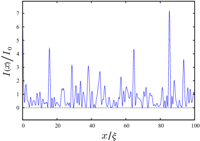
Figure 1: (Color online) The typical 1D (repulsive) blue-detuned speckle profile. The intensity is given in units of $I_{0}$ and the coordinate in units of $\xi$.

Once the electric field correlation function (1) is known, the statistical properties of the intensity are completely determined. This is discussed in the next section, where we consider the statistics of extrema of this correlated and non-Gaussian potential, relevant for the motion of a particle in a random landscape ledoussal03 . By using this description, we derive the DOS and compare the analytical predictions with the spectrum computed numerically for a randomly generated speckle pattern.

To generate the speckle potential profile we use the mathematical counterpart of the mechanism that gives rise to optical speckles. The constructive or destructive interference of randomly phased elementary components of the radiation field caused by the roughness of the scattering surface occurs also in the discrete Fourier transform of a sample function of a random process goodman . This effect can be exploited to generate numerically a speckle pattern with the statistical properties discussed earlier huntley ; modugno06 . Then, the spectrum of the system can be computed numerically by mapping the stationary Schrödinger equation $H\psi=E\psi$ on a discretized grid numerical . All the results presented in this article have been obtained for a system of length $L=600\xi$ and are averaged over a number of realizations ranging from $10^{2}$ to $10^{3}$.

III Statistical analysis of the speckle potential

The typical shape of the potential profile created by a blue-detuned speckle pattern is shown in Fig. 1. The potential profile can be seen as series of peaks (maxima) statistically distributed around the typical value of the order of $I_{0}$. The peaks are separated by valleys of typical width $\xi$ with minima situated most probably near the lower-boundary of the potential. For the red-detuned case the picture is analogous, with the roles of maxima and minima exchanged. In other words, the statistics of the potential minima for the red-detuned case is that of the maxima of the blue-detuned one.

We are interested in the density of minima $n_{\rm min}\left(I^{\prime}\right)$ and the density of maxima $n_{\rm max}\left(I^{\prime}\right)$, at specified intensity $I^{\prime}$, in the spatial distribution $I(x)$ of intensities along the image line. Using the method of Weinrib and Halperin Weinrib82 , the number of minima or maxima can be calculated from the integrated joint probability,

$$N_{\rm min,max}={\int}dx\leavevmode\nobreak\ \delta\left({I_{x}}\right){\Big{|}}{I_{xx}}{\Big{|}}\Theta\left({\pm I_{xx}}\right),$$

where the plus (minus) sign refers to minima (maxima) and we have used the conventions ${\partial I}/{\partial x}\equiv I_{x}$ and ${\partial^{2}I}/{\partial x^{2}}\equiv I_{xx}$. It follows that the density of minima (maxima) per unit length and intensity can be written as

$$n_{\rm min,max}\left(I^{\prime}\right)=\langle\delta\left({I_{x}}\right)\delta\left(I^{\prime}-I\right){|}{I_{xx}}{|}\Theta\left({\pm I_{xx}}\right)\rangle.$$ (6)

In order to evaluate the statistical average of Eq. (6), we need to calculate the joint probability of $I$, $I_{x}$ and $I_{xx}$ (all at the same point) starting from the joint probability of the Gaussian random variables ${\cal E}$, ${\cal E}_{x}$, and ${\cal E}_{xx}$. Because ${\cal E}(x)$ is statistically homogeneous along the $x$ coordinate, the density in Eq. (6) will be independent of position.

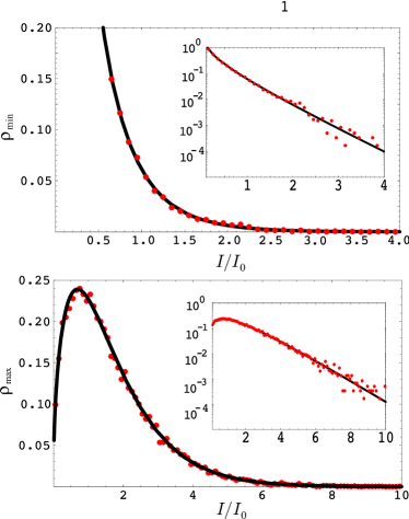
Figure 2: (Color online) Density $\rho(I/I_{0})$ of minima (top) and maxima (bottom) for a blue-detuned speckle (in log scale in the insets). The solid lines represent the analytical prediction of Eq. (III), while the dots have been obtained by averaging over $100$ numerical speckle realizations.

The statistics of a set of Gaussian variables is completely determined by the two-point correlations $G(x-y)$ between them. The nonzero correlators evaluated at the same point are calculated by considering the derivatives of $G(x-y)$. One finds $\langle|{\cal E}|^{2}\rangle=G(0),\langle{\cal E}_{xx}{\cal E}^{\ast}\rangle=-\langle|{\cal E}_{x}|^{2}\rangle=G_{xx}(0),\langle|{\cal E}_{xx}|^{2}\rangle=G_{xxxx}(0)$ with

$$G(0) =I_{0},$$ (7)

$$G_{xx}(0) =-{I_{0}}/{\tilde{\xi}^{2}},$$ (8)

$$G_{xxxx}(0) ={I_{0}}/(\kappa\leavevmode\nobreak\ \tilde{\xi}^{4}),$$ (9)

where we have introduced the length $\tilde{\xi}\equiv\sqrt{3}/(\pi D)$ for convenience. The dimensionless parameter

$$\kappa=\frac{G_{xx}^{2}(0)}{G(0)G_{xxxx}(0)}$$ (10)

is restricted in one dimension to the range $0\leq\kappa\leq 1$. It depends only on the the shape of the correlation function of the electric field but not on the length scale $\xi$. For the correlator of the laser speckle given by Eq. (1), we have $\kappa=5/9$.

On dimensional grounds, it is clear that the density of minima (maxima) of Eq. (6) scales as

$$n_{\rm min,max}(I,\tilde{\xi},\kappa)=\left({1}/{(I_{0}\tilde{\xi}})\right)\rho_{\rm min,max}\left({I}/{I_{0}},\kappa\right).$$ (11)

Evaluating the statistical average in Eq. (6) and rewriting in terms of dimensionless intensity measured in units of $I_{0}$, we obtain

$$\rho_{\rm min,max} \left({\tilde{I}},\kappa\right)=\frac{e^{-\frac{\tilde{I}}{1-\kappa}}}{4\pi^{3/2}}\frac{1}{\tilde{I}^{1/2}\sqrt{\kappa^{-1}-1}}$$

$$\times \int_{-\infty}^{\infty}d\theta_{x}\leavevmode\nobreak\ f(\tilde{I},\theta_{x})\int_{0}^{\infty}d\tilde{I}_{xx}\leavevmode\nobreak\ g(\tilde{I},\theta_{x},\tilde{I}_{xx}),$$ (12)

where $f=\exp\left[-\tilde{I}\theta_{x}^{2}\left(\theta_{x}^{2}-3+\kappa^{-1}\right)/\left(\kappa^{-1}-1\right)\right]$,
$g=\tilde{I}_{xx}\leavevmode\nobreak\ \exp{\left\{-\tilde{I}_{xx}\left[\left({\tilde{I}_{xx}}/{4\leavevmode\nobreak\ \tilde{I}}\right)\mp{\left(\theta_{x}^{2}-1\right)}\right]/\left(\kappa^{-1}-1\right)\right\}}$, and the plus (minus) sign refers to the minima (maxima). The details of the derivation are given in the Appendix. The densities (III) are plotted in Fig. 2. The agreement with the numerical simulation is excellent.

The asymptotic behavior of the integrals in Eq. (III) can be also evaluated analytically. This is useful because the distribution of the deep negative-energy wells of the red-detuned speckle potential is related to the large $I$ asymptotic tail of the maxima distribution of the blue-detuned speckle. This latter behaves for $\kappa=5/9$ as

$${\rho_{\rm max}}(\tilde{I}) \approx \frac{e^{-2\tilde{I}}}{2\pi}\left(2+\frac{e^{\tilde{I}}\left(-1+2\tilde{I}\right)\sqrt{\pi}\leavevmode\nobreak\ {\rm erf}[\tilde{I}]}{\sqrt{\tilde{I}}}\right)$$ (13)

$$\approx {\sqrt{\frac{\tilde{I}}{\pi}}}e^{-\tilde{I}}.$$

Near the boundary of the blue-detuned speckle potential the density of minima diverges as

$${\rho_{\rm min}}(\tilde{I})\approx{1}/{2\sqrt{\pi\tilde{I}}}.$$ (14)

However, in the thermodynamic limit, the DOS of a particle in disordered potential bounded from below is expected to vanish at the boundary. Hence, the correlation between the DOS and the number of minima has to be rather weak.

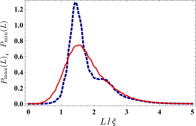
Figure 3: (Color online) The normalized distributions of distance measured in units of the autocorrelation length $\xi$ between neighboring maxima (dotted line) and between neighboring minima (solid line).

More likely, the DOS near the boundary of the spectrum is associated with the distribution of distance between neighboring minima $P_{\mathrm{min}}(L)$ and neighboring maxima $P_{\mathrm{max}}(L)$. It is known that the presence of Lifshitz tails in the DOS for a bounded-from-below potential is related to the existence of large regions free of disorder for the binary distribution or large regions with negligible potential for continuous distributions. In the case of blue-detunded speckle potential, the zero intensity is the most probable so that one would expect that such regions are not so rare. Some idea about their statistical properties can be gained through the distributions of distances between minima and maxima, which can be computed numerically. The normalized distributions of the distance between maxima and between minima are shown in Fig. 3. The average distance for the both distribution is $\langle L\rangle=1.78\leavevmode\nobreak\ \xi$. This value can be easily obtained by integrating the density in Eq. (III) over all the intensities and by assuming that the points of minima (or maxima) are homogeneously distributed. The right tails of both distributions can be well fitted in the window $L/\xi\in[3,5.5]$ by simple exponentials:

$$P_{max}(L) \approx 2.081e^{-1.933(L/\xi)},$$ (15)

$$P_{min}(L) \approx 3.385e^{-2.036(L/\xi)}.$$ (16)

The exponentially small probability of existence of a region of size $L$ with relatively small intensity accounts for the Lifshitz tail in the DOS of the blue detuned speckle potential.

IV DOS: red-detuned speckle

We consider first the DOS for a particle in the red-detuned speckle potential, which corresponds to $s<0$. We discuss separately three different regimes, ranging from the semiclassical limit, for $s\rightarrow-\infty$, down to the quantum regime, when $|s|\leq 1$.

By varying the parameter $s$ the characteristic extension of the localized states differs considerably. In Fig. 4 we present the lowest-lying eigenstates for three different intensities of the same speckle profile, corresponding to $s=-0.1,\ -1,\ -100$. This picture shows that for shallow potentials (the quantum regime) the eigenstates extend over several potential wells. The lowest-lying eigenstates localize inside deep wells. However, the ground state is not necessarily localized in the deepest well since the width of the well plays also a crucial role. As the speckle intensity is increased, the eigenstate width shrinks and their positions may change. Eventually, for large enough $|s|$, the eigenstates tend to stack up as bound states inside isolated wells, with the ground state being the lowest eigenstate of the deepest well (semiclassical regime).

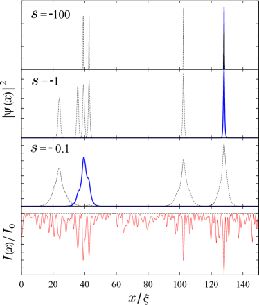
Figure 4: (Color online) Probability density distribution of the lowest lying eigenstates of a red-detuned speckle pattern (bottom panel) for three different intensities corresponding to $s=-0.1,\ -1,\ -100$. Only a window of length $150\xi$ of the whole system is shown. The figure shows the ground state (blue solid line) and several first excited states (black dashed line). Note that, as the speckle intensity changes, the position of the eigenstates may change and some may move in or out from the selected window.

IV.1 Semiclassical regime

In the limit $s\rightarrow-\infty$ the low-energy tail of the DOS is determined by deep isolated states occupying single wells of typical size $\xi$. Therefore, for $E<0$, the DOS can be calculated in the semiclassical approximation Kane63

$$\nu_{|s|\rightarrow\infty}(E)=\frac{1}{I_{0}}\int_{-\infty}^{{E}}\nu_{0}(E-I)\leavevmode\nobreak\ e^{-{{|I|}}/I_{0}}\leavevmode\nobreak\ dI,$$ (17)

where $\nu_{0}(z)={\sqrt{m}}/{\sqrt{2}\pi\hbar\sqrt{z}}$ is the density of state of the continuum in one dimension. Integrating over the intensity in Eq. (17) we find

$$\nu_{|s|\rightarrow\infty}(E)=\sqrt{\frac{m}{2\pi\hbar^{2}I_{0}}}e^{-|E|/I_{0}}.$$ (18)

The DOS in the negative-energy tail predicted by Eq. (18) is in excellent agreement with the curve obtained in the numerical simulation as shown in Fig. 5. Note that this result differs from the DOS of a long-range correlated Gaussian potential that, sufficiently deep in the tail, has the form $\nu(E)\sim\exp(-\mathrm{const}|E|^{2})$ Pastur88 .

The semiclassical result of Eq. (18) can be also understood in terms of the density of minima of the red-detuned speckle potential. Since the latter is the blue-detuned speckle potential taken with negative sign, the distribution of minima is nothing but $n_{\rm max}$, namely, the distribution of maxima of Eq. (6) studied in Sec. III. We assume that each deep state occupies an isolated single well associated with the corresponding minimum of the potential. This approximation is not true in general but is valid for deep enough states. The potential inside of the well can be completely described by derivatives taken at the bottom of the well, denoted by $\{I\}:=\{I,I_{x}=0,I_{xx},I_{xxx},...\}$. Each well is characterized by $M\left[\{I\}\right]$ bound states with energies $E_{n}$, $n=1,\dots,M$, which can be found from the solution of the Schrödinger equation for the particle in the potential $I(x)=-(I+\frac{1}{2}I_{xx}x^{2}+\frac{1}{6}I_{xxx}x^{3}+...)$.

The DOS can be then calculated by summing over all levels in each well and over all wells as follows

$$\nu(E)=\int d\{I\}\!\!\sum_{n=0}^{M\left[\{I\}\right]}n_{\rm min}^{\rm red}\left(\{I\}\right)\delta\left(E-E_{n}\left[\{I\}\right]\right).$$ (19)

For large $\xi$ the typical wells which dominate the DOS at large negative energies can be considered within a harmonic approximation by setting $I(x)\simeq-I-\frac{1}{2}I_{xx}\leavevmode\nobreak\ x^{2}$, with $I_{xx}<0$ so that the resulting spectrum corresponds to a quantum oscillator with the frequency $\omega=\sqrt{-{I_{xx}}/{m}}$. The summation over $n$ can be taken to infinity because in the limit $|s|\rightarrow\infty$ the levels of the harmonic oscillator approach a continuum. Therefore, for $E<0$ we can approximate (19) as

$${\nu_{\rm HO}}\left(E\right)\simeq$$

$$\sum_{n=0}^{\infty}\langle\delta\left({I_{x}}\right)\delta\left(-I+\hbar\omega(n+\frac{1}{2})-E\right){\Big{|}}{I_{xx}}{\Big{|}}\Theta\left(-{I_{xx}}\right)\rangle.\ \ \ \$$ (20)

We have computed the statistical average and carried out the summation over $n$ in Eq. (IV.1) by summing over large numbers of states. The obtained curve is found to be exactly on the top of the semiclassical curve of Eq. (18) shown in Fig. 5. Corrections beyond the harmonic approximation and/or correlations between different points could be taken into account, including higher-order derivatives of $I(x)$ at the bottoms of wells.

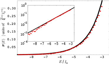
Figure 5: (Color online) Large negative-energy DOS expressed in units of $(\tilde{\xi}I_{0})^{-1}$ in the presence of a red-detuned speckle potential with $s=-2000$ as a function of the rescaled energy $E/I_{0}$ in linear scale and in logarithmic scale (inset). The dots represent the numerical data (averaged over $100$ realizations), while the solid line indicates the analytical semiclassical curve (18).

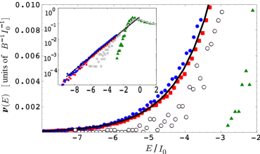
Figure 6: (Color online) The dots represent the numerical data in linear scale and in logarithmic scale (inset) for the low-energy DOS tails in units of $(BI_{0})^{-1}$ in a red-detuned speckle potential as a function of $E/I_{0}$ for different values $s<0$: $s=-2000$ (red squares), $s=-1000$ (blue circles), $s=-1$ (open circles) and $s=-0.1$ (green triangles). The black solid line refers to the analytical semiclassical result (18) valid at large $|s|$.

IV.2 Intermediate regime

Upon decreasing $|s|$ the quasiclassical approximation becomes inadequate, as shown in Fig. 6. In general, at sufficiently large negative energies $E\ll E_{\xi}$, the DOS is determined by the deep wells of size $\lambda\leq\xi$ no matter how short the correlation length $\xi$ is john84 . At higher energies $E\geq E_{\xi}$, the wave function of the localized state is spread over more than one typical fluctuation of the disorder potential, that is, $\lambda\geq\xi$. This picture is supported by the numerical analysis of the spatial extension of the localized states in the low-energy tail. As one can see from Fig. 4 the wave functions for $s=-0.1$ corresponding to the energy range shown in Fig. 6 spread over a region $\lambda\gg\xi$. The same analysis for $s=-1$ reveals that the typical extension of the wave function for the low-energy states is of the same order as $\xi$. Note that, since the condition $E\ll E_{\xi}$ corresponds to $E/I_{0}\ll-1/|s|$, it is not possible to see the transition to the deep localized levels at $E\ll E_{\xi}$ from the data of Fig. 6 for $|s|<1$.

Here we study the low-energy tail of the DOS for moderate values of $|s|\sim 1$. This value occurs typically in the experiments with cold atoms in optical speckles fallani08 . In this regime the semiclassical approximation breaks down due to quantum-mechanical effects despite that the interaction between different wells remains negligible. The decrease of $|s|$ results in a depletion of the DOS seen in Fig. 6. This effect can simply be explained by the reduction of the number of levels in each potential well. In the harmonic approximation (19), one does indeed find that decreasing $\xi$ at fixed $B$ leads to an increase of the distance between levels. Alternatively, reducing $I_{0}$ at fixed $\xi$ causes a shrinking of the interlevel distance which is counterbalanced by a larger decreasing of the wells depth. Thus, the decrease of $s$ always corresponds to a reduction of the number of bound states in each well.

In this case we cannot rely on the infinite-sum approximation. Taking into account only a ground state in each well severely underestimates the DOS. Keeping any constant finite upper limit $M[\{I\}]$ in the sum over levels remains inadequate due to a quite broad distribution of the number of bound states in different wells. A different approach has to be considered. One method is to extend the semiclassical approximation given by Eq. (17) in order to include quantum effects. To this end it is useful to introduce the 1D cumulated DOS Lloyd75 ${\cal D}(E,V)=\left({\sqrt{2m}}/{\pi\hbar}\right)\sqrt{E-V}$ which is related to the total number of states in a well of size $\lambda$ created at the minimum $V_{\rm min}=-I_{\rm max}$ of the potential $V(x)=-I(x)$,

$$N(E,V_{\rm min})=\left({\sqrt{2m}}/{\pi\hbar}\right)\sqrt{E-V_{\rm min}}\leavevmode\nobreak\ \lambda.$$

The condition to have at least one state requires that this number is larger than 1, that is, $0>E\geq V_{\rm min}+\hbar^{2}/2m\lambda^{2}$. This can be incorporated in the cumulative DOS by shifting the energy zero Lloyd75 :

$${\cal D}(E,V_{\rm min})=\frac{\sqrt{2m}}{\pi\hbar}\sqrt{E-V_{\rm min}-\frac{\hbar^{2}}{2m\lambda^{2}}}.$$ (21)

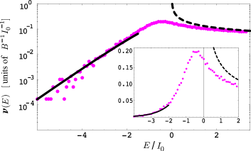
Figure 7: (Color online) The dots represent the DOS for a red-detuned speckle potential with $s=-1$ in logarithmic scale and in linear scale (inset). The solid line describes the modified semiclassical approximation of Eqs. (22)-(24) with $\beta=0.5$ valid in the low-energy tail. At positive energies, the DOS approaches asymptotically the 1D continuum $\nu_{0}(E)=\sqrt{m}/\pi\hbar\sqrt{2\leavevmode\nobreak\ E}$, indicated by the dashed line.

Changing from the cumulated DOS to the DOS we arrive at

$$\nu_{|s|\sim 1}(E,\lambda)=\frac{\sqrt{m}}{\sqrt{2}\pi\hbar}\int_{-\infty}^{E-\frac{\hbar^{2}}{2m\lambda^{2}}}\frac{{\tilde{P}}[-V]}{\sqrt{E-V-\frac{\hbar^{2}}{2m\lambda^{2}}}}\leavevmode\nobreak\ dV,$$ (22)

where ${\tilde{P}}[-I]$ is the normalized probability distribution function of minima of the red-detuned speckle potential, so that ${\tilde{P}}[I]$ is the similar distribution of maxima of the blue-detuned speckle:

$${\tilde{P}}[I]=\frac{n_{\rm max}(I,\xi,\kappa)}{\int_{0}^{\infty}n_{\rm max}(I^{\prime},\xi,\kappa)\leavevmode\nobreak\ d{I^{{}^{\prime}}}}.$$ (23)

Moreover, because we know that the extension of the wave function of these states does not exceed the typical size of the potential wells, we can take the energy of the localized state proportional to the zero-point energy inside the well, that is,

$${\hbar^{2}}/{2m\lambda^{2}}\sim\beta\leavevmode\nobreak\ |E|,$$ (24)

where the parameter $\beta$ cannot be determined exactly within this method. However the result is not extremely sensitive to the choice of $\beta$ in the limits $0<\beta<1$. Choosing the value $\beta\sim 0.5$ the modified semiclassical method based on Eqs. (22) and (23) reproduces very well the data for $s=-1$, as shown in Fig. 7. We also tried to fit the computed DOS by a stretched exponential. We found that it cannot be done well in the whole window of numerical data. However, in smaller windows it can be fitted by a stretch exponential with the exponent varying between 1 and 1.5 and weakly depending on $\beta$.

IV.3 Quantum limit

When the correlation length of the disorder $\xi$ is reduced to $|s|\leq 1$, the wave function of the localized states in the low-energy tail $-1/|s|<E/I_{0}<0$ is spread over a distance $\lambda$ larger than the typical distance between two minima (see Fig. 4). Therefore, the probability of constructing a local wave function is not directly related to the probability distribution of the bare potential $P[I]$ or that of its extrema $\tilde{P}[I]$. The interplay between different wells has to be taken into account as well. This can be done by considering the probability $P_{\lambda}[I]$ of the potential integrated over the characteristic extension $\lambda(E)$ of the state of energy $E$ Lifshitz68 .

For finite $\lambda(E)>\xi$ we can divide the region occupied by the wave function into $n=\lambda(E)/\xi$ parts, which are approximately uncorrelated. Assuming that the correlation inside each part is strong enough we can approximately replace the distribution of potential integrated over the correlation length $P_{\xi}[I]$ by the bare distribution (2). Then the distribution integrated over the width of wave function $P_{\lambda}[I]$ can be computed using the characteristic function method. The characteristic function is defined as $f(t)=\langle e^{itI}\rangle$ so that $f_{\lambda}(t)=[f_{\xi}(t/n)]^{n}$. This gives

$$P_{\lambda}[I]=\frac{1}{I_{0}}\frac{n^{n}}{\Gamma(n)}\left(\frac{I}{I_{0}}\right)^{n-1}e^{-nI/I_{0}},$$ (25)

with $n=\lambda(E)/\xi$. It can be shown that for very large $\lambda$ the integrated exponential distribution (25) approaches asymptotically a Gaussian law:

$$P_{\lambda}[I]\stackrel{{\scriptstyle\lambda\gg 1}}{{\sim}}\frac{\sqrt{\lambda}}{\sqrt{2\pi}I_{0}\sqrt{\xi}}\exp{\left(-\frac{\lambda(I-I_{0})^{2}}{2I_{0}^{2}\xi}\right)}.$$ (26)

By reversing the argument, we can say that for a given energy there is an optimal well of size $\lambda$ created by the average potential $V$, which may bind a state whose zero-point energy should not be larger than $\hbar/2m\lambda^{2}$. Therefore, the negative low-energy tail of the DOS can be calculated with a variational principle from Lloyd75

$$\nu_{|s|\ll 1}(E,\lambda)\sim\frac{\sqrt{m}}{\sqrt{2}\pi\hbar}\int_{-\infty}^{E-\frac{\hbar^{2}}{2m\lambda^{2}}}\frac{{P}_{\lambda}[-V]}{\sqrt{E-V-\frac{\hbar^{2}}{2m\lambda^{2}}}}\leavevmode\nobreak\ dV.$$ (27)

By making the variation with respect to $\lambda$, for large negative energies $|E|\gg I_{0}$, we find that the DOS of Eq. (27) goes asymptotically as

$$\nu_{|s|\ll 1}(E)\sim\exp{\left(-\frac{8\sqrt{3}}{9\sqrt{2}}\frac{\hbar|E|^{3/2}}{\sqrt{m}\xi I_{0}^{2}}\right)}.$$ (28)

The limit $s\rightarrow 0^{-}$ of very short disorder correlation length corresponds thus to the white-noise potential

$$\langle V(x)V(x^{\prime})\rangle_{P_{\lambda}}=\kappa_{0}^{2}\delta(x-x^{\prime}),$$

where $\kappa_{0}^{2}\equiv I_{0}^{2}\xi$ has to remain finite as $\xi\rightarrow 0$. Therefore, we see that the asymptotic DOS (28) reproduces the typical Lifshitz tail law for unbounded delta-correlated potential

$$\nu_{|s|\ll 1}(E)\sim\exp{\left(-\frac{2\sqrt{3}}{9}\left(\frac{|E|}{{E}_{\rm L}}\right)^{3/2}\right)},$$ (29)

where ${E}_{\rm L}=\left(m\kappa_{0}^{4}/\hbar^{2}\right)^{1/3}/2$ is nothing but the 1D Larkin energy Falco08 ; Falco09 .

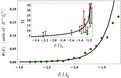
Figure 8: (Color online) The dots show the low-energy DOS tail computed numerically for a particle in red-detuned speckle potential with $s=-0.1$. The black solid line corresponds to the variational result of Eq. (27) with $P_{\lambda}[I]$ given by Eq. (25). The inset shows the number of wells occupied by the states as a function of energy. The green squares and red circles are computed for the first few states in a particular speckle sample using the attenuation factor of 10 and 100, respectively. The solid line is the prediction of the variational calculations.

In Fig. 6 we show some numerical results for the systems with values of $s$ down to $s=-0.1$. For such a small value of $|s|$, the typical wave-functions of the states in the low-energy tail are spread over a distance a few times larger than the typical distance between neighboring wells. These states are not yet sufficiently extended in order to reach for the distribution of $P_{\lambda}[I]$ the asymptotic Gaussian probability shape of Eq. (26). The probability distribution $P_{\lambda}[I]$ given by Eq. (25) lies somewhere between the exponential law (2) and the Gaussian curve of Eq. (26). To compute the DOS for moderately small $s$, we substitute Eq. (25) into Eq. (27) and minimize it with respect to the number of occupied wells $n=\lambda/\xi$. This gives the result which interpolates between the semiclassical result of Eq. (22) and the Lifshitz tail (29). The corresponding DOS computed for $s=-0.1$ is shown in Fig. 8 together with numerical data. The variational prediction for the number of occupied states is shown in the inset. The dots in the inset depict the number of occupied wells for the first few states in a particular speckle sample. To estimate this number from the numerical data we calculate the width of each wave function using the criterion of the amplitude attenuation by factors of 10 and 100. We find a good agreement with the results of the variational calculation.

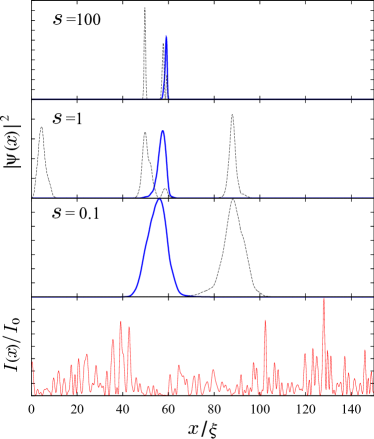
Figure 9: (Color online) Probability density distribution of the lowest lying eigenstates of a blue-detuned speckle pattern (in the bottom panel), for three different intensities with $s=0.1,\ 1,\ 100$. Only a window of length $150\xi$ of the whole system is shown. The figure shows the ground state (blue solid line) and several first excited states (black dashed line).

V DOS: blue-detuned speckle

The random potential created by a blue-detuned laser speckle is bounded from below so that the DOS vanishes at energies lower than the natural boundary $E_{0}=0$. Analogously to the red-detuned problem, the localized region of the spectrum is controlled by the parameter $s$. The lowest-lying eigenstates for three different intensities of the same speckle profile, corresponding to $s=0.1,1$, and $100$ are depicted in Fig. 9. This picture shows that with decreasing $s$ the wave functions extend over larger numbers of potential wells.

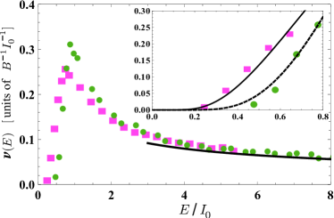
Figure 10: (Color online) The one particle DOS for a blue-detuned speckle potential computed numerically for $s=0.1$ (greed circles) and $s=1$ (magenta squares). The black solid line is the DOS of free particle. Inset. The best simultaneous fit of the Lifshitz tail of both DOS by Eq. (36) with the same $c_{0}=0.8141$ and $A=0.4098$.

V.1 Small $s$ limit

The DOS computed numerically for $s=0.1$ and $s=1$ are shown in Fig. 10. At large energies the DOS approaches the limit of free particle while at small energies it exhibits the Lifshitz’s tail behavior. It is well known that the DOS near the bottom of a bounded-from-below disorder potential is controlled by the existence of very large regions “free” of disorder potential. The probability of their appearance in the speckle pattern can be estimated as follows.

We assume the existence of a bound state with energy $E$ localized inside this region. In general, this region has the average intensity that is not exactly zero but well below the energy level $E$. Since we are interested in the asymptotic low energy behavior, we can fix the largest intensity to $E\ll I_{0}$. However, very small intensity corresponds also to a vanishing electric field. The probability to have a region of size $L$ with the electric field in the interval between ${\cal E}(x)$ and ${\cal E}(x)+d{\cal E}(x)$ is given by

$$\!\!\!\!\!\!\!\!\!dW[{\cal E}(x),d{\cal E}(x)]$$

$$=\exp\left[-\int\limits_{0}^{L}{\cal E}^{*}(x)G^{-1}(x-x^{\prime}){\cal E}(x^{\prime})dxdx^{\prime}\right]$$

$$\times(\det G)^{-1}\prod\limits_{x\in[0,L]}\frac{d{\cal E}(x)d{\cal E}^{*}(x)}{\pi a_{0}},$$ (30)

where $a_{0}$ is the UV cutoff and the inverse correlator is defined by

$$\int dx^{\prime\prime}G(x-x^{\prime\prime})G^{-1}(x^{\prime\prime}-x^{\prime})=\delta(x-x^{\prime}).$$ (31)

The Fourier transform of the electric field correlator (1) reads

$$\tilde{G}(k)=I_{0}/D\,\Theta({\pi}\,D-|k|),$$ (32)

where $\Theta(x)$ is the Heaviside step function. In what follows, we use $D\sim 1/\xi$ absorbing the numerical factor of $0.88$ into the overall coefficient. For small $s$ the eigenstates spread over distance $L$ much larger than the typical well width $\xi$. In this regime $\det G$ can be estimated using Eq. (32) as follows:

$$\det G=\prod\limits_{k=-\pi/\xi}^{-\pi/L}I_{0}\xi\prod\limits_{k=\pi/L}^{\pi/\xi}I_{0}\xi=(I_{0}\xi)^{2L/\xi}.$$ (33)

Substituting this into Eq. (V.1) and putting ${\cal E}(x)=0$ in the exponential gives the probability for the region of size $L$ to have the electric field in the interval between $0$ and $d{\cal E}(x)=E^{1/2}e^{i\theta}$, where $\theta$ is arbitrary. Integrating out $\theta$ and summing over $x$ we obtain

$$W[0,E^{1/2}]\sim(I_{0}\xi)^{-2L/\xi}(2E/a_{0})^{2L/a_{0}}.$$ (34)

Since we are interested in the leading exponential behavior, we can replace in Eq. (34) $a_{0}$ by $\xi$ and arrive at

$$W[0,E^{1/2}]\sim\exp\left[-\frac{2L}{\xi}\ln\left(\frac{I_{0}}{E}\right)\right].$$ (35)

The region being almost free of disorder has a bound state with energy $E=c_{0}^{2}\hbar^{2}/(2mL^{2})$, where $c_{0}$ is a constant of order $1$. Using the latter in Eq. (35) to express $L$ in terms of $E$, we obtain the Lifshitz’s tail for the energy distribution as

$$\nu(E)\approx A\exp\left[-c_{0}s^{-1/2}\sqrt{\frac{I_{0}}{E}}\ln\left(\frac{I_{0}}{E}\right)\right].$$ (36)

The logarithmic corrections to the Lifshitz tail of the same form as in Eq. (36) was found for the uncorrelated disorder by mapping the problem to the random walk of a classical particle in a medium with traps politi88 and using a variational approach luck89 . We fit using Eq. (36) the lower energy tail of the DOS computed numerically for $s=0.1$ and $s=1$. The corresponding curves are shown in the inset of Fig. 10. We find that taking into account the logarithmic corrections is necessary in order to fit the data in the energy interval that is accessible numerically.

V.2 Large $s$ limit

The DOS computed numerically for $s=100,1000$, and $2000$ are shown in Fig. 11. The DOS exhibits a quite flat crossover region between the narrow Lifshitz’s tail and the large energy asymptotic behavior corresponding to the free particle. For general $s$ the Lifshitz tail of the DOS is expected to have the form

$$\nu(E)\sim\exp\left[-c_{0}\sqrt{{I_{0}}/{E}}\,{\cal F}\left(s,\ln\left({I_{0}}/{E}\right)\right)\right],$$

where ${\cal F}(s,t)$ is a universal function depending only on the form of $G(x)$. Fitting the DOS computed numerically (see inset of Fig. 11) we find that for $s\in[100,2000]$ this function can be approximated by ${\cal F}(s,t)\approx s^{-1/4}\,t$. Thus, the correlations in the speckle potentials growing with $s$ renormalize the effective exponent of $s$ in the exponential of the Lifshitz tail.

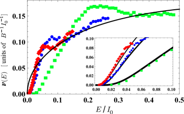
Figure 11: (Color online) The DOS of a particle in a blue-detuned speckle potential are computed numerically for $s=2000$ (red diamond), $s=1000$ (blue circles) and $s=100$ (green squares). The black solid line refers to the analytical semiclassical result (V.2) valid at large $s$ and $E/{I_{0}}\gtrsim 1/\sqrt{s}$. Inset. The best simultaneous fit of the Lifshitz tail of three DOS by $\nu(E)\approx A\exp\left[-c_{0}s^{-1/4}\sqrt{I_{0}/E}\ln(I_{0}/E)\right]$ with the same $c_{0}=0.6375$ and $A=0.3425$.

To compute the DOS in the crossover regime, we use the semiclassical approximation and obtain

$$\nu_{s\rightarrow\infty}(E)= \frac{1}{I_{0}}\int_{0}^{E}\nu_{0}(E-I)\leavevmode\nobreak\ e^{-I/I_{0}}\leavevmode\nobreak\ dI$$

$$= \sqrt{\frac{m}{2\pi\hbar^{2}I_{0}}}e^{-E/I_{0}}{\rm erfi}\left[\sqrt{\frac{E}{I_{0}}}\right],$$ (37)

where ${\rm erfi}(x)$ is the imaginary error function. The DOS (V.2) goes asymptotic as $\sim\nu_{0}(E)$ for large positive energies. Near the boundary of the spectrum $E\rightarrow 0$ it behaves as

$$\nu_{s\rightarrow\infty}(E)=\frac{1}{\pi}\sqrt{\frac{2m}{\hbar^{2}I_{0}}}\sqrt{\frac{E}{I_{0}}}.$$

The comparison between Eq. (V.2) and the numerical data data in Fig. 11 shows that there is a range of energies where the two results agree quite well.

V.3 Effective mobility edge

The possible existence of the effective mobility edge in 1D systems with certain correlated disorder has been considered in several works izrailev99 ; lugan09 . It is expected, for example, for the potentials with correlations having a finite support in Fourier space. In particular as follows from Eq. (32) the speckle potential has no Fourier components with $|k|>\pi/D$. As a result, in the Born approximation there is no backscattering for particles with momentum larger than $\hbar k>\hbar\pi/D$ that defines the effective mobility edge. The localization length above this edge is determined by corrections to the Born approximations and larger by one order of magnitude. In our unities the effective mobility edge is expected at

$$E_{\rm M}=I_{0}[1+(0.88\pi)^{2}/s],$$ (38)

which gives $E_{\rm M}/I_{0}\approx 8.64$ for $s=1$ and $E_{\rm M}/I_{0}\approx 1.008$ for $s=1000$. At these energies the DOS is already very close to the DOS of a free particle. One cannot see any signature of the effective mobility edge like it happens with the DOS and the real mobility edge in higher dimensions. To probe the effective mobility edge, one has to study the asymptotic behavior of the wave functions at this energy sanchez07 which is beyond of the scope of this article.

VI Summary

In this work we have studied the DOS of a quantum particle in a laser-speckle potential using the statistics of the speckle potential profile and numerical simulations. The DOS in the speckle potential can be characterized by a single parameter $s$, which depends on the correlation length of the disorder, the average value of the laser intensity and the mass of the particles. We have considered both cases of red-detuned and blue-detuned potentials for which the random potential is bounded from above and from below, respectively.

For the negative-energy region of DOS in the red-detuned speckle there are three different regimes: semiclassical ($|s|\gg 1$), intermediate ($|s|\sim 1$), and quantum ($|s|<1$). For strongly correlated disorder, $|s|\gg 1$, the tail of the DOS is related to the statistical distribution of the deep minima of the disorder potential. In the quantum limit with $|s|<1$, the DOS is controlled by smoothing effects leading to the Lifshitz tail of uncorrelated Gaussian potential. In the crossover regime, $|s|\sim 1$, the DOS can be described within the semiclassical approach by including quantum corrections.

In the case of a blue-detuned speckle potential, the DOS near the bottom of the spectrum is given by the Lifshitz tail related to the existence of large regions with negligible intensity. We have found logarithmic corrections to the celebrated Lifshitz result due to the continuous nature of the distribution of the potential. The relevance of these corrections for typical setup parameters in current experiments is supported by our numerical results.

Appendix A

Because $E_{x}$ has nonzero correlations only with itself, the total joint probability in Eq. (6) can be written as

$$p(E,E_{x},E_{xx})=p(E_{x})p(E,E_{xx}).$$ (39)

In rescaled unities of $I_{0}$ and $\tilde{\xi}$ we can immediately write

$$p(E_{x})\equiv{(\pi^{2}\langle E_{x}^{\ast}E_{x}\rangle)^{-1/2}}e^{-\frac{|E_{x}|^{2}}{\langle E_{x}^{\ast}E_{x}\rangle^{2}}}={\pi^{-1}}e^{-{|E_{x}|^{2}}}.$$ (40)

The joint probability for the two correlated variables $E$ and $E_{xx}$ can be written using matrix representation as

$$p(E,E_{xx})=\left(\pi^{2}{\rm det}\leavevmode\nobreak\ {{\bf M}}\right)^{-1}e^{-{{\bf A}}^{\dagger}{\bf M}^{-1}{\bf A}},$$ (41)

with ${\bf A}^{\dagger}=(E^{*},E^{*}_{xx})$ and

$${\bf M}\equiv\left(\begin{array}[]{cc}\langle EE^{\ast}\rangle&\langle EE_{xx}^{\ast}\rangle\\ \langle E_{xx}E^{\ast}\rangle&\langle E_{xx}E_{xx}^{\ast}\rangle\end{array}\right)=\left(\begin{array}[]{cc}1&-1\\ -1&\kappa^{-1}\end{array}\right),$$ (46)

which has an inverse matrix that reads

$${\bf M}^{-1}=\frac{1}{\kappa^{-1}-1}\left(\begin{array}[]{cc}\kappa^{-1}&1\\ 1&1\end{array}\right).$$ (49)

Equation (41) can be rewritten as

$$p(E,E_{xx})=\frac{\pi^{-2}}{\kappa^{-1}-1}e^{-\frac{1}{\kappa^{-1}-1}\left(|E|^{2}\kappa^{-1}+|E_{xx}|^{2}+2{{\cal R}e\left[E^{\ast}E_{xx}\right]}\right)}.$$

Using the following variable transformation $E(x)\equiv\sqrt{I(x)}\leavevmode\nobreak\ e^{i\theta(x)}$ and setting $I_{x}=0$, we obtain

$$E_{x}= i\theta_{x}I^{1/2}e^{i\theta(x)}$$ (50)

$$E_{xx}= \left(\frac{I_{xx}}{2I^{1/2}}-I^{1/2}\theta_{x}^{2}\right)e^{i\theta}+i\theta_{xx}I^{1/2}e^{i\theta}.$$ (51)

Therefore, the joint probability (39) can be written as

$$p(E,E_{x},E_{xx})=J_{0}\leavevmode\nobreak\ p(\theta,\theta_{x},\theta_{xx},I,I_{x}=0,I_{xx}),$$ (52)

where

$$p (\theta,\theta_{x},\theta_{xx},I,I_{x}=0,I_{xx})=\frac{\pi^{-3}}{\kappa^{-1}-1}$$ (53)

$$e^{-I\theta_{x}^{2}-\frac{1}{\kappa^{-1}-1}\left[\kappa^{-1}I+\left(\frac{I_{xx}}{2I^{1/2}}-I^{1/2}\theta_{x}^{2}\right)^{2}+I\theta_{xx}^{2}+I_{xx}-2I\theta_{x}^{2}\right]},$$

and the Jacobian is $J_{0}=2^{-3}$. Integration over $\theta$ yields a factor $2\pi$. We can also analytically integrate out $I$ and $\theta_{xx}$, which is a Gaussian integral. As a result, we arrive at Eq. (III).

References

- (1) J. W. Goodman, Speckle Phenomena: Theory and Applications, Roberts and Company Publishers (2007).
- (2) D. Boiron, C. Mennerat-Robilliard, J.-M. Fournier, L. Guidoni, C. Salomon, and G. Grynberg, Eur. Phys. J. D 7, 373 (1999).
- (3) J. E. Lye, L. Fallani, M. Modugno, D. S. Wiersma, C. Fort, and M. Inguscio, Phys. Rev. Lett. 95, 070401 (2005).
- (4) D. Clément, A.F. Varon, M. Hugbart, J.A. Retter, P. Bouyer, L. Sanchez-Palencia, D.M. Gangardt, G.V. Shlyapnikov and A. Aspect, Phys. Rev. Lett. 95, 170409 (2005).
- (5) C. Fort, L.Fallani, V. Guarrera, J. E. Lye, M. Modugno, D. S. Wiersma, and M. Inguscio, Phys. Rev. Lett. 95, 170410 (2005).
- (6) T. Schulte et al., Phys. Rev. Lett. 95, 170411 (2005).
- (7) M. Modugno, Phys. Rev. A 73, 013606 (2006).
- (8) L. Sanchez-Palencia, Phys. Rev. A 74, 053625 (2006).
- (9) D. Clément, A.F. Varon, J.A. Retter, L. Sanchez-Palencia, A. Aspect and P. Bouyer, New J. of Physics 8, 165 (2006).
- (10) P. Lugan, D. Clement, P. Bouyer, A. Aspect, and L. Sanchez-Palencia, Phys. Rev. Lett. 99, 180402 (2007).
- (11) Yong P. Chen, J. Hitchcock, D. Dries, M. Junker, C. Welford, and R. G. Hulet, Phys. Rev. A 77, 033632 (2008).
- (12) L. Sanchez-Palencia, D. Clément, P. Lugan, P. Bouyer, G.V. Shlyapnikov and A. Aspect, Phys. Rev. Lett. 98, 210401 (2007).
- (13) J. Billy, V. Josse, Z. Zuo, A. Bernard, B. Hambrecht, P. Lugan, D. Clément, L. Sanchez-Palencia, P. Bouyer and A. Aspect, Nature (London) 453, 891 (2008).
- (14) A related experiment with quasiperiodic disorder has been reported in: G. Roati et al., Nature (London) 453, 895 (2008).
- (15) L. Sanchez-Palencia, D. Clément, P. Lugan, P. Bouyer, and A. Aspect, New J. Phys. 10, 045019 (2008).
- (16) D. Dries, S. E. Pollack, J. M. Hitchcock, and R. G. Hulet, Phys. Rev. A 82, 033603 (2010).
- (17) M. P. A. Fisher, P. B. Weichman, G. Grinstein, and D. S. Fisher, Phys. Rev. B 40, 546 (1989).
- (18) F. Zhou, Phys. Rev. B 73, 035102 (2006).
- (19) S. O. Diallo, J. V. Pearce, R. T. Azuah, O. Kirichek, J. W. Taylor, and H. R. Glyde, Phys. Rev. Lett. 98, 205301 (2007).
- (20) G. M. Falco, T. Nattermann, and V. L. Pokrovsky, Europhys. Lett. 85, 30002 (2009).
- (21) V. Gurarie, L. Pollet, N. V. Prokof’ev, B. V. Svistunov, and M. Troyer, Phys. Rev. B 80, 214519 (2009).
- (22) L. Fontanesi, M. Wouters, and V. Savona, Phys. Rev. A 81, 053603 (2010).
- (23) E. Altman, Y. Kafri, A. Polkovnikov, and G. Refael, Phys. Rev. B 81, 174528 (2010).
- (24) B. Deissler, M. Zaccanti, G. Roati, C. D’Errico, M. Fattori, M. Modugno, G. Modugno, and M. Inguscio, Nature Physics 6, 354 (2010).
- (25) R. C. Kuhn, C. Miniatura, D. Delande, O. Sigwarth, and C. A. Müller, Phys. Rev. Lett. 95, 250403 (2005).
- (26) R. C. Kuhn, O. Sigwarth, C. Miniatura, D. Delande and C. A. Müller, New J. Phys. 9, 161 (2007).
- (27) P. Henseler and B. Shapiro, Phys. Rev. A 77, 033624 (2008).
- (28) S. Pilati, S. Giorgini, and N. Prokof’ev, Phys. Rev. Lett. 102, 150402 (2009); S. Pilati, S. Giorgini, M. Modugno, and N. Prokof’ev, New J. Phys. 12, 073003 (2010).
- (29) I. M. Lifshits, S. A. Gradeskul, and L. A. Pastur, Introduction to the Theory of Disordered Systems (Wiley, New York, 1988).
- (30) B. Kramer and A. MacKinnon, Rep. Prog. Phys. 56, 1469 (1993).
- (31) J. M. Huntley, Appl. Opt. 28, 4316 (1989). P. Horak, J.-Y. Courtois, and G. Grynberg, Phys. Rev. A 58, 3953 (1998).
- (32) L. Fallani, C. Fort, and M. Inguscio, Adv. At. Mol. Opt. Phys. 56, 119 (2008).
- (33) G. M. Falco, T. Nattermann, and V. L. Pokrovsky, Phys. Rev. B 80, 104515 (2009); There, for the correlation length of the disorder, the symbol is used instead of .
- (34) P. Le Doussal and C. Monthus, Physica A 317, 140 (2003).
- (35) We use the following prescription: , with vanishing boundary conditions, . The number of grid points is 8192.
- (36) A. Weinrib and B. I. Halperin, Phys. Rev. B 26, 1362 (1982).
- (37) E. O. Kane, Phys. Rev. 131, 79 (1963).
- (38) S. John and M. J. Stephen, J. Phys. C 17, L559 (1984).
- (39) P. Lloyd and P. R. Best, J. Phys. C 8, 3752 (1975).
- (40) I. M. Lifshitz, Zh. Eksp. Teor. Fiz. 53, 743 (1967) [Sov. Phys. JETP 26, 462 (1968)].
- (41) G. M. Falco, J. Phys. B: At. Mol. Opt. Phys. 42, 215303 (2009).
- (42) A. Politi and T. Schneider, Europhys. Lett. 5, 715 (1988).
- (43) T.M. Nieuwenhuizen and J.M. Luck, Europhys. Lett. 9, 407 (1989).
- (44) F. M. Izrailev and A. A. Krokhin, Phys. Rev. Lett. 82, 4062 (1999).
- (45) P. Lugan, A. Aspect, L. Sanchez-Palencia, D. Delande, B. Grémaud, C. A. Müller, and C. Miniatura, Phys. Rev. A80, 023605 (2009).