Effects of Electromagnetic Field on the Dynamics of Bianchi type $VI_{0}$ Universe with Anisotropic Dark Energy

Abstract

Spatially homogeneous and anisotropic Bianchi type $VI_{0}$ cosmological models with cosmological constant are investigated in the presence of anisotropic dark energy. We examine the effects of electromagnetic field on the dynamics of the universe and anisotropic behavior of dark energy. The law of variation of the mean Hubble parameter is used to find exact solutions of the Einstein field equations. We find that electromagnetic field promotes anisotropic behavior of dark energy which becomes isotropic for future evolution. It is concluded that the isotropic behavior of the universe model is seen even in the presence of electromagnetic field and anisotropic fluid.

Keywords: Electromagnetic Field; Dark Energy; Anisotropy.
PACS: 04.20.Jb; 04.20.Dw; 04.40.Nr; 98.80.Jk

1 Introduction

The most remarkable advancement in cosmology is its observational evidence which says that our universe is in an accelerating expansion phase. Supernova $I_{a}$ data [1, 2] gave the first indication of the accelerated expansion of the universe. This was confirmed by the observations of anisotropies in the cosmic microwave background (CMB) radiation as seen in the data from satellite such as WMAP [3] and large scale structure [4]. Today’s one of the major concerns of cosmology is the dark energy. Recent cosmological observations [1, 2, 3, 4] suggest that our universe is (approximately) spatially flat and its cosmic inflation is due to the matter field (dark energy) having negative pressure (violating energy conditions). The composition of universe density is the following: 74% dark energy (DE), 22% dark matter and 4% ordinary matter [5]. Though there is a compelling evidence that expansion of the universe is accelerating, yet the nature of dark energy has been under consideration since the last decade [6]-[10]. Several models have been proposed for this purpose, e.g., Chaplygin gas, phantoms, quintessence, cosmological constant and dark energy in brane worlds. However, none of these models can be regarded as being entirely convincing so far.

The cosmological constant, $\Lambda$ is the most obvious theoretical candidate of DE which has the equation of state (EoS) $\omega=-1$. Astronomical observations indicate that the cosmological constant is many orders of magnitude smaller than estimated in modern theories of elementary particles [11]. Stabell and Refsdal [12] discussed the evolution of Friedmann-Lema$\hat{i}$tre Robertson and Walker (FLRW) dust models in the presence of positive cosmological constant. These results are given in a more generalized form [13, 14] using the general EoS. Wald [15] examined the late time behavior of expanding homogeneous cosmological models satisfying the Einstein field equations (EFEs) with a positive cosmological constant. He found that all the Bianchi type models except $IX$ showed isotropic behavior. These models exponentially evolve towards the de Sitter universe with a scale factor $(3/{\Lambda})^{1/2}$. Goliath and Ellis [16] used the dynamical system methods to observe the spatially homogeneous cosmological models with a cosmological constant. The inclusion of cosmological constant provides an effective mean of isotropizing homogeneous universes [15, 16].

The presence of magnetic fields in galatic and intergalatic spaces is evident from recent observations [17]. The large scale magnetic fields can be detected by observing their effects on the CMB radiation. These fields would enhance anisotropies in the CMB, since the expansion rate will be different depending on the directions of the field lines [18, 19]. Matravers and Tsagas [20] found that interaction of the cosmological magnetic field with the spacetime geometry could affect the expansion of the universe. If the curvature is strong, then even the weak magnetic field will effect the evolution of the universe. The magneto-curvature coupling tends to accelerate the positively curved regions while it decelerates the negatively curved regions [20, 21].

Jacobs [22] studied the spatially homogeneous and anisotropic Bianchi type $I$ cosmological model with expansion and shear but without rotation. He discussed anisotropy in the temperature of CMB and expansion both with and without magnetic field. It was concluded that the primordial magnetic field produced large expansion anisotropies during the radiation-dominated phase but it had negligible effect during the dust-dominated phase. Dunn and Tupper [23] discussed properties of Bianchi type $VI_{0}$ models with perfect fluid and magnetic field. Roy et al. [24] explored the effects of cosmological constant in Bianchi type $I$ and $VI_{0}$ models with perfect fluid and homogeneous magnetic field in the axial direction. They found that model expanded for negative values of the cosmological constant while it contracted for positive $\Lambda$. In a recent paper [25], Sharif and Shamir explored the vacuum solution of Bianchi $I$ and $V$ models in $f(R)$ gravity.

Rodrigues [26] proposed Bianchi $I$ with a non-dynamical DE component which yields anisotropic vacuum pressure in two ways: (i) by considering the anisotropic vacuum consistent with energy-momentum conservation; (ii) by implementing a Poisson structure deformations between canonical momenta such that re-scaling of scale factors is not violated. Koivisto and Mota [27] have investigated a cosmological model containing the DE fluid with non-dynamical anisotropic EoS and interacts with perfect fluid. They suggested that if the DE EoS is anisotropic, the expansion rate of the universe becomes direction dependent at late times and cosmological models with anisotropic EoS can explain some of the observed anomalies in CMB.

Recently, Akarsu and Kilinc [28] investigated anisotropic Bianchi type $I$ models in the presence of perfect fluid and minimally interacting DE with anisotropic EoS parameter. They found that anisotropy of the DE did not always promote anisotropy of the expansion. The anisotropic fluid may support isotropization of the expansion for relatively earlier times in the universe. The same authors [29] have worked on the Bianchi type $III$ model in the presence of single imperfect fluid with dynamical anisotropic EoS parameter and dynamical energy density. They observed that anisotropy of the expansion vanished and hence the universe approached isotropy for late times of the universe in accelerating models.

It would be worthwhile to see what happens if we consider the electromagnetic field with anisotropic DE. The main purpose of this work is to look at the effects of electromagnetic field on the dynamics of the universe in the presence of anisotropic DE for Bianchi type $VI_{0}$. The layout of the paper is as follows. In section 2 we describe spatially homogeneous and anisotropic Bianchi type $VI_{0}$ spacetime and formulate the EFEs in the presence of anisotropic fluid and magnetic field. Section 3 presents a special law of variation for the mean Hubble parameter which yields constant deceleration parameter. This law generates two types of solutions: power law and exponential expansion. In section 4, a hypothetical form of fluid is obtained by making an assumption on anisotropy of the fluid. We obtain exact solutions of the EFEs and discuss physical behavior of anisotropic DE and universe model. Finally, section 5 concludes the results.

2 Model and the Field Equations

The spatially homogeneous and anisotropic Bianchi type $VI_{0}$ model is described by the line element

$$ds^{2}=dt^{2}-A^{2}(t)dx^{2}-e^{2mx}B^{2}(t)dy^{2}-e^{-2mx}C^{2}(t)dz^{2},$$ (1)

where scale factors $A,~{}B$ and $C$ are functions of cosmic time $t$ only, $m\neq 0$ is a constant. The energy-momentum tensor for the electromagnetic field is given as [30]

$$T_{\mu}^{\nu(em)}=\bar{\mu}[|h|^{2}(u_{\mu}u^{\nu}-1/2\delta_{\mu}^{\nu})-h_{\mu}h^{\nu}],$$ (2)

where $u^{\nu}$ is the four-velocity vector satisfying

$$g_{\mu\nu}u^{\mu}u^{\nu}=1.$$ (3)

$\overline{\mu}$ is the magnetic permeability and $h_{\mu}$ is the four-magnetic flux given by

$$h_{\mu}=\frac{\sqrt{-g}}{2\overline{\mu}}\varepsilon_{{\mu}{\nu}{\alpha}{\beta}}F^{{\alpha}{\beta}}u^{\nu},\quad(\mu,\nu,\alpha,\beta=0,1,2,3)$$ (4)

where $\varepsilon_{{\mu}{\nu}{\alpha}{\beta}}$ is the Levi-Civita tensor, $F^{{\alpha}{\beta}}$ is the electromagnetic field tensor and $|h|^{2}=h_{\nu}h^{\nu}$. We assume that magnetic field is due to an electric current produced along $x$-axis and thus it is in $yz$-plane. In co-moving coordinates $u^{\nu}=(1,0,0,0)$ and hence Eq.(4) gives $h_{1}\neq 0,~{}h_{0}=h_{2}=h_{3}=0$. Using these values in Eq.(4), it follows that $F_{12}=F_{13}=0,~{}F_{23}\neq 0.$

The electric and magnetic field in terms of field tensor are defined as [31]

$$E_{\mu}=F_{{\mu}{\nu}}u^{\nu},\quad B_{\mu}=\frac{1}{2}\varepsilon_{{\mu}{\nu}{\alpha}}F^{{\nu}{\alpha}}.$$ (5)

According to Ohm’s law, we have

$$h_{{\mu}{\nu}}J^{\nu}={\sigma}F_{{\mu}{\nu}}u^{\nu},$$ (6)

where $h_{{\mu}{\nu}}=g_{{\mu}{\nu}}+u_{\mu}u_{\nu}$ is the projection tensor orthogonal to $u^{\mu}$, ${\sigma}$ is the conductivity and $J^{\mu}$ is the four current density. In the magnetohydrodynamic limit, conductivity takes infinitely large value while current remains finite so that $E_{\mu}\rightarrow 0$ [31]. Consequently, Eq.(5) leads to $F_{01}=F_{02}=F_{03}=0.$ Thus the only non-vanishing component of electromagnetic field tensor $F_{{\mu}{\nu}}$ is $F_{23}$. The Maxwell’s equations

$$F_{{\mu}{\nu};{\alpha}}+F_{{\nu}{\alpha};{\mu}}+F_{{\alpha}{\mu};{\nu}}=0,\quad F^{{\mu}{\nu}}_{{;}{\alpha}}=0$$ (7)

are satisfied by

$$F_{23}=K=constant.$$ (8)

It follows from Eq.(4) that

$$h_{1}=\frac{AK}{\overline{\mu}BC},\quad|h|^{2}=\frac{K^{2}}{{\overline{\mu}}^{2}B^{2}C^{2}}.$$ (9)

Using this equation in Eq.(2), we obtain

$$T_{0}^{{0}{(em)}}=\frac{K^{2}}{2\overline{\mu}B^{2}C^{2}}=T_{1}^{{1}{(em)}}=-T_{2}^{{2}{(em)}}=-T_{3}^{{3}{(em)}}.$$

Thus we have

$$T_{\mu}^{{\nu}{(em)}}=diag[\frac{K^{2}}{2\overline{\mu}B^{2}C^{2}},\frac{K^{2}}{2\overline{\mu}B^{2}C^{2}},-\frac{K^{2}}{2\overline{\mu}B^{2}C^{2}},-\frac{K^{2}}{2\overline{\mu}B^{2}C^{2}}].$$ (10)

The energy-momentum tensor for anisotropic DE fluid is taken in the following form [28, 29]

$$T_{\mu}^{\nu}=diag[\rho,-p_{x},-p_{y},-p_{z}]$$ (11)

This model of the DE is characterized by the EoS, $p=\omega{\rho}$, where $\omega$ is not necessarily constant [33]. From Eq.(11), we have

$$T_{\mu}^{\nu}=diag[1,-({\omega}+{\delta}),-{\omega},-({\omega}+{\gamma})]\rho,$$ (12)

where $\rho$ is the energy density of the fluid; $p_{x}$, $p_{y}$ and $p_{z}$ are pressures and $\omega_{x},~{}\omega_{y},~{}\omega_{z}$ are directional EoS parameters on $x,~{}y$ and $z$ axes respectively. The deviation from isotropy is obtained by setting

$${\omega}_{x}={\omega}+{\delta},\quad{\omega}_{y}={\omega},\quad{\omega}_{z}={\omega}+{\gamma},$$

where $\omega$ is the deviation free EoS parameter and $\delta$ and $\gamma$ are the deviations from $\omega$ on $x$ and $z$ axes respectively. The EFEs with cosmological constant are given by

$$G_{{\mu}{\nu}}=R_{{\mu}{\nu}}-\frac{1}{2}Rg_{{\mu}{\nu}}-{\Lambda}g_{{\mu}{\nu}}=8\pi(T_{{\mu}{\nu}}+T_{{\mu}{\nu}}^{(em)}),$$ (13)

where $R_{{\mu}{\nu}}$ is the Ricci tensor, R is the Ricci scalar, $T_{{\mu}{\nu}}$ is the energy-momentum tensor for anisotropic fluid and $T_{{\mu}{\nu}}^{(em)}$ is the energy-momentum tensor for the electromagnetic field.

For Bianchi type $VI_{0}$ spacetime, the EFEs become

$$\frac{\dot{A}\dot{B}}{AB}+\frac{\dot{A}\dot{C}}{AC}+\frac{\dot{B}\dot{C}}{BC}-\frac{m^{2}}{A^{2}}=8{\pi}{\rho}+\frac{4{\pi}K^{2}}{\overline{\mu}B^{2}C^{2}}+{\Lambda},$$ (14)

$$\frac{\ddot{B}}{B}+\frac{\ddot{C}}{C}+\frac{\dot{B}\dot{C}}{BC}+\frac{m^{2}}{A^{2}}=-8{\pi}({\omega}+{\delta}){\rho}+\frac{4{\pi}K^{2}}{\overline{\mu}B^{2}C^{2}}+{\Lambda},$$ (15)

$$\frac{\ddot{A}}{A}+\frac{\ddot{C}}{C}+\frac{\dot{A}\dot{C}}{AC}-\frac{m^{2}}{A^{2}}=-8{\pi}{\omega}{\rho}-\frac{4{\pi}K^{2}}{\overline{\mu}B^{2}C^{2}}+{\Lambda},$$ (16)

$$\frac{\ddot{A}}{A}+\frac{\ddot{B}}{B}+\frac{\dot{A}\dot{B}}{AB}-\frac{m^{2}}{A^{2}}=-8{\pi}({\omega}+{\gamma}){\rho}-\frac{4{\pi}K^{2}}{\overline{\mu}B^{2}C^{2}}+{\Lambda},$$ (17)

$$m(\frac{\dot{B}}{B}-\frac{\dot{C}}{C})=0,$$ (18)

where dot denotes derivative with respect to time $t$. Equation (18) yields

$$B=c_{1}C,$$ (19)

where $c_{1}$ is a constant of integration. Subtracting Eq.(17) from (16) and using (19), we obtain ${\gamma}=0$ which shows that directional EoS parameters $\omega_{y},~{}\omega_{z}$ and the pressures $p_{y},~{}p_{z}$ become equal. Using Eq.(19) and ${\gamma}=0$, the EFEs (14)-(17) reduce to the following set of equations

$$2\frac{\dot{A}\dot{B}}{AB}+\frac{\dot{B}^{2}}{B^{2}}-\frac{m^{2}}{A^{2}} = 8{\pi}{\rho}+\frac{4{\pi}K^{2}}{\overline{\mu}k_{1}^{2}B^{4}}+{\Lambda},$$ (20)

$$2\frac{\ddot{B}}{B}+\frac{\dot{B}^{2}}{B^{2}}+\frac{m^{2}}{A^{2}} = -8{\pi}({\omega}+{\delta}){\rho}+\frac{4{\pi}K^{2}}{\overline{\mu}k_{1}^{2}B^{4}}+{\Lambda},$$ (21)

$$\frac{\ddot{A}}{A}+\frac{\ddot{B}}{B}+\frac{\dot{A}\dot{B}}{AB}-\frac{m^{2}}{A^{2}} = -8{\pi}{\omega}{\rho}-\frac{4{\pi}K^{2}}{\overline{\mu}k_{1}^{2}B^{4}}+{\Lambda}.$$ (22)

3 Some Physical and Geometrical Parameters

Here we discuss some physical and geometrical quantities for the Bianchi type $VI_{0}$ model which are important in cosmological observations. The average scale factor is given by

$$a=(k_{1}AB^{2})^{\frac{1}{3}}$$ (23)

while the volume is defined as

$$V=a^{3}=k_{1}AB^{2}.$$ (24)

The mean Hubble parameter $H$ and the directional Hubble parameters $H_{i}(i=1,2,3)$ in $x,~{}y$ and $z$ directions are

$$H=\frac{1}{3}({\ln}V\dot{)}={\ln}\dot{a}=\frac{1}{3}(\frac{\dot{A}}{A}+2\frac{\dot{B}}{B}),\quad H_{x}=\frac{\dot{A}}{A},\quad H_{y}=H_{z}=\frac{\dot{B}}{B}.$$ (25)

The physical parameters such as scalar expansion $\Theta$, shear scalar $\sigma^{2}$ and anisotropy of the expansion $\Delta$ are given as follows

$$\Theta = u_{;a}^{a},$$ (26)

$$\sigma^{2} = \frac{1}{2}\sigma_{ab}\sigma^{ab},$$ (27)

$$\Delta = \frac{1}{3}\sum_{i=1}^{3}(\frac{H_{i}-H}{H})^{2}.$$ (28)

The anisotropy of expansion shows isotropic behavior for $\Delta=0$.

It is mentioned here that any universe model becomes isotropic for the diagonal energy-momentum tensor when $t\rightarrow{+\infty},~{}\Delta\rightarrow 0,~{}V\rightarrow{+\infty}$ and $T^{00}>0~{}(\rho>0)$ [29, 32]. The law of variation of mean Hubble parameter is given as

$$H=la^{-n}=l(k_{1}AB^{2})^{-n/3},$$ (29)

where $l>0$ and $n\geqslant 0$. This law was initially proposed by Berman [34] for spatially homogeneous and isotropic RW spacetime which yields constant value of the deceleration parameter. In recent papers [28, 35], a similar law is proposed for the homogeneous and anisotropic Bianchi models to generate exact solutions.

The volumetric deceleration parameter $q$ is the measure of rate at which expansion of the universe slows down due to self-gravitation. It is defined as

$$q=-\frac{a\ddot{a}}{\dot{a}^{2}}.$$ (30)

Using Eqs.(25) and (29), we get

$$\dot{a}=la^{-n+1},\quad\ddot{a}=-l^{2}(n-1)a^{-2n+1}$$ (31)

which gives constant values of the deceleration parameter as follows

$$q = n-1\quad for\quad n\neq 0,$$

$$q = -1\quad for\quad n=0.$$

Recent observations show that expansion rate of the universe is accelerating which may be due to the presence of DE and $q<0$. Thus the sign of $q$ indicates whether the cosmological model inflates or not. For $q>0$ (i.e. $n>1$), the model represents decelerating universe where as the negative sign ${-1}{\leqslant}q{<}0$ for $0{\leqslant}n{<}1$ indicates inflation and $q=0$ for $n=1$ corresponds to expansion with constant velocity. Equations (25) and (29) yield two different volumetric expansion laws

$$V = k_{2}e^{3lt},\quad n=0,$$ (32)

$$V = (nlt+c)^{3/n},\quad n\neq 0$$ (33)

which are used to find exact solutions of the EFEs. In fact these represent two different models of the universe.

4 Solution of the Field Equations

We can find the most general form of anisotropy parameter for the expansion of Bianchi type $VI_{0}$ in the presence of anisotropic fluid and electromagnetic field using Eq.(25). The anisotropy parameter of expansion can be written as

$$\Delta=\frac{2}{9H^{2}}(H_{x}-H_{y})^{2},$$ (34)

where $H_{x}-H_{y}$ is the difference between the expansion rates on $x$ and $y$ axes which can be found using the field equations.

Subtracting Eq.(22) from (21) and after some manipulation, it follows that

$$\frac{\dot{A}}{A}-\frac{\dot{B}}{B}=\frac{d}{V}+\frac{1}{V}\int{(8\pi{\delta}{\rho}+\frac{2m^{2}}{A^{2}}-\frac{8{\pi}K^{2}}{k_{1}^{2}\overline{\mu}B^{4}})Vdt},$$ (35)

where $d$ is another constant of integration. Now using this equation in Eq.(34), the anisotropy parameter takes the form

$$\Delta=\frac{2}{9H^{2}}[d+\int{(8\pi{\delta}{\rho}+\frac{2m^{2}}{A^{2}}-\frac{8{\pi}K^{2}}{k_{1}^{2}\overline{\mu}B^{4}})Vdt}]^{2}V^{-2}.$$ (36)

The anisotropy parameter in the presence of isotropic fluid can be obtained by choosing $\delta=0$ which yields

$$\Delta=\frac{2}{9H^{2}}[d+\int{(\frac{2m^{2}}{A^{2}}-\frac{8{\pi}K^{2}}{k_{1}^{2}\overline{\mu}B^{4}})Vdt}]^{2}V^{-2}.$$ (37)

We take the value of $\delta$ so that the integrand in the above equation vanishes

$$\delta=-\frac{m^{2}}{4{\pi}{\rho}A^{2}}+\frac{K^{2}}{k_{1}^{2}\overline{\mu}{\rho}{B^{4}}}.$$ (38)

The corresponding energy-momentum tensor for anisotropic DE fluid turns out to be

$$T_{\mu}^{\nu}=diag[1,-({\omega}-\frac{m^{2}}{4{\pi}{\rho}A^{2}}+\frac{K^{2}}{k_{1}^{2}\overline{\mu}{\rho}{B^{4}}}),-{\omega},-{\omega}]\rho.$$ (39)

The anisotropy parameter of the expansion reduces to

$$\Delta=\frac{2}{9}\frac{d^{2}}{H^{2}}V^{-2}.$$ (40)

We see that $\Delta$ obtained for the Bianchi type $VI_{0}$ in the presence of anisotropic fluid with electromagnetic field is equivalent to that found for the Bianchi type $III$ in the presence of anisotropic fluid [29].

The difference between the directional Hubble parameters becomes

$$H_{x}-H_{y}=\frac{d}{V}.$$ (41)

The most general form of the energy density is found by using Eqs.(20) and (28) as

$$\rho=\frac{1}{8{\pi}}[3H^{2}(1-\frac{\Delta}{2})-\frac{m^{2}}{A^{2}}-{\Lambda}-\frac{4{\pi}K^{2}}{\overline{\mu}k_{1}^{2}B^{4}}].$$ (42)

This shows that anisotropy of expansion, cosmological constant and electromagnetic field reduce the energy density $\rho$ of anisotropic DE.

4.1 Model for $n=0~{}(q=-1$)

The spatial volume of the universe for this model is given by

$$V=k_{2}e^{3lt}.$$ (43)

Using this value of $V$ in Eq.(41) and then solving the EFEs (20)-(22), the scale factors become

$$A = k_{3}e^{lt-\frac{2}{9}\frac{d}{lk_{2}}e^{-3lt}},$$ (44)

$$B = (\frac{k_{2}}{k_{1}k_{3}})^{\frac{1}{2}}e^{lt+\frac{1}{9}\frac{d}{lk_{2}}e^{-3lt}},$$ (45)

$$C = (\frac{k_{1}k_{2}}{k_{3}})^{\frac{1}{2}}e^{lt+\frac{1}{9}\frac{d}{lk_{2}}e^{-3lt}},$$ (46)

where $k_{1},~{}k_{2}$ and $k_{3}$ are constants of integration.

The directional and the mean Hubble parameters will become

$$H_{x}=l+\frac{2}{3}\frac{d}{k_{2}}e^{-3lt},\quad H_{y}=H_{z}=l-\frac{1}{3}\frac{d}{k_{2}}e^{-3lt},\quad H=l$$ (47)

while the anisotropy parameter of the expansion takes the form

$$\Delta=\frac{2}{9}\frac{d^{2}}{l^{2}k_{2}^{2}}e^{-6lt}.$$ (48)

The expansion and shear scalar are found as

$$\Theta = u_{;a}^{a}=\frac{\dot{A}}{A}+2\frac{\dot{B}}{B}=3l=3H,$$ (49)

$$\sigma^{2} = \frac{1}{2}[(\frac{\dot{A}}{A})^{2}+2(\frac{\dot{B}}{B})^{2}]-\frac{1}{6}{\Theta}^{2}=\frac{1}{3}\frac{d^{2}}{k_{2}^{2}}e^{-6lt}.$$ (50)

The energy density of the DE is evaluated by using Eq.(20) with the scale factors as

$$\rho = \frac{1}{8\pi}[3l^{2}-\Lambda-\frac{1}{3}\frac{d^{2}}{k_{2}^{2}}e^{-6lt}-\frac{m^{2}}{k_{3}^{2}}e^{-2lt+\frac{4}{9}\frac{d}{lk_{2}}e^{-3lt}}-\frac{4{\pi}K^{2}}{\overline{\mu}}(\frac{k_{3}^{2}}{k_{2}^{2}})$$ (51)

$$\times e^{-4lt-\frac{4}{9}\frac{d}{lk_{2}}e^{-3lt}}].$$

The deviation free part of anisotropic EoS parameter $\omega$ can be obtained by using Eqs.(44)-(46) and (51) in Eq.(21)

$$\omega = \{9k_{2}^{2}k_{3}^{2}l^{2}+d^{2}k_{3}^{2}e^{-6lt}-3{\Lambda}k_{2}^{2}k_{3}^{2}-3m^{2}k_{2}^{2}e^{-2lt+\frac{4}{9}\frac{d}{lk_{2}}e^{-3lt}}+\frac{12{\pi}k_{3}^{4}K^{2}}{\overline{\mu}}$$ (52)

$$\times e^{-4lt-\frac{4}{9}\frac{d}{lk_{2}}e^{-3lt}}\}/\{d^{2}k_{3}^{2}e^{-6lt}+3{\Lambda}k_{2}^{2}k_{3}^{2}-9k_{2}^{2}k_{3}^{2}l^{2}+3m^{2}k_{2}^{2}$$

$$\times e^{-2lt+\frac{4}{9}\frac{d}{lk_{2}}e^{-3lt}}+\frac{12{\pi}k_{3}^{4}K^{2}}{\overline{\mu}}e^{-4lt-\frac{4}{9}\frac{d}{lk_{2}}e^{-3lt}}\}.$$

Using the scale factors and the energy density in Eq.(38), the deviation in EoS parameter along $x$-axis $\delta$ is given as

$$\delta = \{6m^{2}k_{2}^{2}e^{-2lt+\frac{4}{9}\frac{d}{lk_{2}}e^{-3lt}}+\frac{24{\pi}K^{2}k_{3}^{4}}{\overline{\mu}}e^{-4lt-\frac{4}{9}\frac{d}{lk_{2}}e^{-3lt}}\}/\{d^{2}k_{3}^{2}e^{-6lt}+3{\Lambda}k_{2}^{2}$$ (53)

$$\times k_{3}^{2}-9k_{2}^{2}k_{3}^{2}l^{2}+3m^{2}k_{2}^{2}e^{-2lt+\frac{4}{9}\frac{d}{lk_{2}}e^{-3lt}}+\frac{12{\pi}k_{3}^{4}K^{2}}{\overline{\mu}}e^{-4lt-\frac{4}{9}\frac{d}{lk_{2}}e^{-3lt}}\}.$$

4.2 Some Physical Aspects of the Model

We find that the directional Hubble parameters are dynamical where as the mean Hubble parameter is constant. Also, the directional Hubble parameters become constant at $t=0$ and when $t\rightarrow{\infty}$. These deviate from the mean Hubble parameter by some constant factor at $t=0$ but coincide when $t\rightarrow{\infty}$. Since the constant is positive (negative), it increases (decreases) expansion on the $x$-axis and it decreases (increases) expansion on $y$ and $z$ axes. The volume $V$ of the universe is finite at $t=0$, expands exponentially with the increase in time $t$ and takes infinitely large value as $t\rightarrow\infty$. Thus the universe evolves with constant volume and expands exponentially. The expansion scalar is constant for $0{\leq}t{\leq}{\infty}$ and hence the model represents uniform expansion.

It is mentioned here that the scale factors $A(t),~{}B(t)$ and $C(t)$ are finite at $t=0$ which implies that the model has no initial singularity whereas these diverge for later times of the universe. The anisotropy parameter of the expansion and shear scalar are found to be finite for earlier times of the universe where as these decrease with time and become zero as $t\rightarrow\infty$. This shows that anisotropy of the expansion is not supported by the anisotropic DE and electromagnetic field. The quantities $\rho,~{}\omega$ and $\delta$ are dynamical and are finite at $t=0$. The deviation free EoS parameter of the DE may begin in the phantom $(\omega<-1)$ or quintessence region $(\omega>-1)$ but $\omega{\rightarrow}-1$ for later times of the universe. One can observe that $\rho$ increases when $\omega$ is in phantom region and attains a constant value as $\omega{\rightarrow}-1$. This is shown in Figure 1.

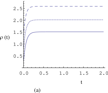
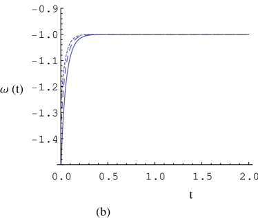
Figure 1: Plot of (a) $\rho(t)$ and (b) $\omega(t)$ verses cosmic time $t$ for $m=1$ and varying values of $l$ as follows: solid, $l=4$; dotted, $l=4.5$; dashed, $l=5$.

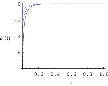
Figure 2: Plot of $\delta$ verses cosmic time $t$ for $m=1$ and varying values of $l$ as follows: solid, $l=4$; dotted, $l=4.5$; dashed, $l=5$.

We see from Eq.(53) that electromagnetic field favors the deviation from $\omega$ on $x$-axis, i.e., it contributes to anisotropic behavior of the fluid. The deviation parameter increases from negative values towards zero with the increase in time and tends to zero as $t\rightarrow{\infty}$ shown in Figure 2. Thus the anisotropic fluid becomes isotropic for the later times of the universe in the case of exponential volumetric expansion. It follows from Eq.(51) that when $t\rightarrow{\infty},~{}{\rho}\rightarrow{3l^{2}-\Lambda}=3H^{2}-\Lambda$ which implies that for $t\rightarrow{\infty},~{}\rho>0$ only if $H>\sqrt{{\Lambda}/3}$ and hence $\Delta{\rightarrow}0$ and $V\rightarrow{\infty}$. Thus the model approaches to isotropy for its future evolution. Here $q=-1,~{}dH/dt=0$ which gives the largest value of the Hubble parameter and accelerating rate of expansion.

4.3 Model for $n\neq 0~{}(q=n-1$)

The initial time of the universe is found by using Eq.(33)

$$t_{*}=-c/nl\quad for\quad n\neq 0.$$ (54)

We re-define the cosmic time as

$$t^{\prime}=nlt+c$$ (55)

such that the initial time turns out to be zero, i.e., $t^{\prime}=0$. For this value of cosmic time, we can re-define the Bianchi model in the form

$$ds^{2}=(nl)^{-2}dt^{\prime 2}-A^{2}(t^{\prime})dx^{2}-e^{2mx}B^{2}(t^{\prime})dy^{2}-e^{-2mx}C^{2}(t^{\prime})dz^{2}.$$ (56)

The corresponding volume will become

$$V=t^{\prime\frac{3}{n}}.$$ (57)

Using this value of $V$ in Eq.(41) and then solving the EFEs (20)-(22), the scale factors turn out to be

$$A(t^{\prime}) = k_{3}t^{\prime\frac{1}{n}}e^{\frac{2}{3}\frac{nd}{n-3}t^{\prime 1-\frac{3}{n}}},$$ (58)

$$B(t^{\prime}) = (\frac{k_{2}}{k_{1}k_{3}})^{\frac{1}{2}}t^{\prime\frac{1}{n}}e^{-{\frac{1}{3}\frac{nd}{n-3}t^{\prime 1-\frac{3}{n}}}},$$ (59)

$$C(t^{\prime}) = (\frac{k_{1}k_{2}}{k_{3}})^{\frac{1}{2}}t^{\prime\frac{1}{n}}e^{-{\frac{1}{3}\frac{nd}{n-3}t^{\prime 1-\frac{3}{n}}}}.$$ (60)

The directional and mean Hubble parameters take the form

$$H=(nt^{\prime})^{-1},\quad H_{x}=\frac{1}{nt^{\prime}}+\frac{2d}{3}t^{\prime-{\frac{3}{n}}},\quad H_{y}=H_{z}=\frac{1}{nt^{\prime}}-\frac{d}{3}t^{\prime-{\frac{3}{n}}}.$$ (61)

The corresponding anisotropy parameter of the expansion turns out to be

$$\Delta=\frac{2}{9}n^{2}d^{2}t^{\prime~{}{2-\frac{6}{n}}}$$ (62)

while the expansion and shear scalar are

$$\Theta=\frac{3}{nt^{\prime}}=3H,\quad\sigma^{2}=\frac{1}{3}d^{2}t^{\prime-\frac{6}{n}}.$$ (63)

The energy density can be found from Eq.(20) by using the scale factors Eq.(58)-(60) as

$${\rho}(t^{\prime}) = \frac{1}{8\pi}[3(nt^{\prime})^{-2}-\Lambda-\frac{1}{3}d^{2}t^{\prime-\frac{6}{n}}-\frac{m^{2}}{k_{3}^{2}}t^{\prime-\frac{2}{n}}e^{-\frac{4}{3}\frac{nd}{n-3}t^{\prime 1-\frac{3}{n}}}-\frac{4{\pi}K^{2}}{\overline{\mu}}$$ (64)

$$\times (\frac{k_{3}^{2}}{k_{2}^{2}})t^{\prime-\frac{4}{n}}e^{\frac{4}{3}\frac{nd}{n-3}t^{\prime 1-\frac{3}{n}}}].$$

Using this equation and the scale factors in Eq.(21), we obtain the deviation free EoS parameter $\omega$

$${\omega(t^{\prime})} = \{(9(nt^{\prime})^{-2}+d^{2}t^{\prime-\frac{6}{n}}-6(nt^{2})^{-1}-3{\Lambda})k_{2}^{2}k_{3}^{2}+3t^{\prime-\frac{4}{n}}e^{\frac{4}{3}\frac{nd}{n-3}t^{\prime 1-\frac{3}{n}}}$$ (65)

$$\times (\frac{4{\pi}k_{3}^{4}K^{2}}{\overline{\mu}}-m^{2}k_{2}^{2}t^{\prime\frac{2}{n}}e^{-\frac{8}{3}\frac{nd}{n-3}t^{\prime 1-\frac{3}{n}}})\}/\{(d^{2}t^{\prime-\frac{6}{n}}+3\Lambda-9(nt^{\prime})^{-2})$$

$$\times k_{2}^{2}k_{3}^{2}+3t^{\prime-\frac{4}{n}}e^{\frac{4}{3}\frac{nd}{n-3}t^{\prime 1-\frac{3}{n}}}(\frac{4{\pi}k_{3}^{4}K^{2}}{\overline{\mu}}+m^{2}k_{2}^{2}t^{\prime\frac{2}{n}}e^{-\frac{8}{3}\frac{nd}{n-3}t^{\prime 1-\frac{3}{n}}})\}.$$

Finally, the deviation parameter $\delta$ can be obtained using the value of ${\rho(t^{\prime})}$ along with Eqs.(58)-(60) in (38)

$${\delta(t^{\prime})} = \{6t^{\prime-\frac{4}{n}}e^{\frac{4}{3}\frac{nd}{n-3}t^{\prime 1-\frac{3}{n}}}(\frac{4{\pi}k_{3}^{4}K^{2}}{\overline{\mu}}+m^{2}k_{2}^{2}t^{\prime\frac{2}{n}}e^{-\frac{8}{3}\frac{nd}{n-3}t^{\prime 1-\frac{3}{n}}})\}/\{(d^{2}t^{\prime-\frac{6}{n}}$$ (66)

$$+ 3\Lambda-9(nt^{\prime})^{-2})k_{2}^{2}k_{3}^{2}+3t^{\prime-\frac{4}{n}}e^{\frac{4}{3}\frac{nd}{n-3}t^{\prime 1-\frac{3}{n}}}(\frac{4{\pi}k_{3}^{4}K^{2}}{\overline{\mu}}+m^{2}k_{2}^{2}t^{\prime\frac{2}{n}}$$

$$\times e^{-\frac{8}{3}\frac{nd}{n-3}t^{\prime 1-\frac{3}{n}}})\}.$$

4.4 Some Physical Aspects of the Model

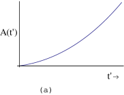
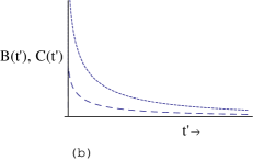
Figure 3: Evolution of (a) $A(t^{\prime})$ and (b) $B(t^{\prime})$ (dashed line), $C(t^{\prime})$ (dotted line) for $n>3,~{}d>0$ as $t^{\prime}\rightarrow{\infty}$.

The universe model accelerates for $0<n<1$, decelerates for $n>1$ and expands with constant velocity for $n=1$. The mean Hubble parameter, shear scalar and directional Hubble parameters are infinite at the initial epoch and tend to zero for later times of the universe. If $n>3,~{}d>0$ then $A(t^{\prime})$ takes infinitely large value while both $B(t^{\prime})$ and $C(t^{\prime})$ vanish as $t^{\prime}\rightarrow{\infty}$. This indicates that spacetime exhibits ”pancake” type singularity which is shown in Figure 3. If $n>3,~{}d<0$, then $A(t^{\prime})$ decreases to zero where as both $B(t^{\prime})$ and $C(t^{\prime})$ continue to increase as $t^{\prime}\rightarrow{\infty}$, leading to a ”cigar” singularity shown in Figure 4. For $n<3$, the scale factors $A(t^{\prime}),~{}B(t^{\prime})$ and $C(t^{\prime})$ become infinite as $t^{\prime}\rightarrow{\infty}$ given in Figure 5.

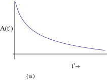
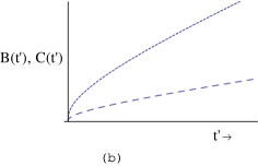
Figure 4: Evolution of (a) $A(t^{\prime})$ and (b) $B(t^{\prime})$ (dashed line), $C(t^{\prime})$ (dotted line) for $n>3$, $d<0$ as $t^{\prime}\rightarrow{\infty}$.

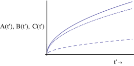
Figure 5: Evolution of $A(t^{\prime})$, solid line; $B(t^{\prime})$ dashed; $C(t^{\prime})$ dotted for $n<3$ as $t^{\prime}\rightarrow{\infty}$.

We note that spatial volume $V$ is zero at $t^{\prime}=0$ and it takes infinitely large value as $t^{\prime}\rightarrow{\infty}$. The expansion scalar is infinite at $t^{\prime}=0$ and decreases with the increase in cosmic time. Thus the universe starts evolving with zero volume at the initial epoch with an infinite rate of expansion and expansion rate slows down for the later times of the universe. The dynamics of anisotropy parameter of the expansion $\Delta$ depends on the value of $n$. $\Delta$ tends to zero as $t^{\prime}\rightarrow{\infty}$ and diverges as $t^{\prime}\rightarrow 0$ for $n<3$ and vice versa for $n>3$ while it remains constant for $n=3$ shown in Figure 6.

Now we determine such values of $n$ which satisfy $\rho>0$ and are suitable for the evolution of the universe. We consider magnetic field, anisotropy of expansion and cosmological constant for the behavior of energy density of the DE. For this purpose, we discuss the following two cases, i.e., $n<3$ and $n>3$. When $n<3$, we have $\rho<0$ as $t^{\prime}\rightarrow 0$ and hence this model is not suitable for representing the relatively earlier times of the universe. When $t^{\prime}\rightarrow{\infty}$, it follows that ${\rho}\geqslant 0$ with ${\Lambda}\leqslant 0$ which is an appropriate model for representing the later times of the universe. For $n>3$, we obtain $\rho<0$ as $t^{\prime}\rightarrow{\infty}$ and it becomes positive as $t^{\prime}\rightarrow 0$. Thus this model can represent the universe only for the earlier times of the universe by assigning suitable values to the constants.

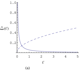
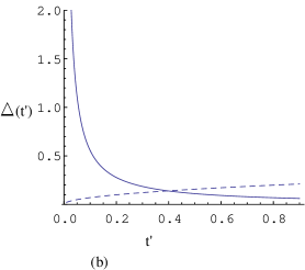
Figure 6: Plot of $\Delta$ verses cosmic time $t^{\prime}$; solid line for $n<3$ and dotted for $n>3$ as (a) $t^{\prime}\rightarrow{\infty}$ (b) $t^{\prime}\rightarrow 0$

If $n<3$ and $\Lambda{\leqslant 0},~{}\rho{\geqslant}0$ (for later times of the universe), $\omega$ begins in quintessence region and then passes into the phantom region. It remains in the phantom region with the increase in time and becomes $-1$ as $t^{\prime}\rightarrow{\infty}$. If $n>3$ with $\rho{\geqslant}0$ (for earlier times of the universe), $\omega$ begins in quintessence region, passes into the phantom region for small interval of time then it passes back into the quintessence region and becomes $-1$ as $t^{\prime}\rightarrow{\infty}$.

Thus we may examine the behavior of anisotropy of the fluid and universe model for $n<3$ with $\Lambda{\leqslant 0}$ and $\rho{\geqslant}0$ as $t^{\prime}\rightarrow{\infty}$. One can observe that magnetic field may increase anisotropic behavior of the DE since it contributes to $\delta$ which decreases with the increase in time and it tends to zero as $t^{\prime}\rightarrow{\infty}$. Thus the anisotropy of the DE vanishes in the presence of magnetic field for later times of the universe with negative cosmological constant. We note that anisotropy parameter of the expansion is not supported by anisotropy of the DE and magnetic field for later times of the universe since for $n<3,~{}\Delta{\rightarrow}0$ as $t^{\prime}\rightarrow{\infty}$. It is observed that $V{\rightarrow}\infty$ and $\rho{\geqslant}0$ as $t^{\prime}\rightarrow{\infty}$ for $n<3$ and hence the model represents isotropic universe for future evolution.

5 Summary and Conclusion

We have obtained two exact solutions of the dynamical equations for the spatially homogeneous and anisotropic Bianchi type $VI_{0}$ model with magnetic field, anisotropic DE and cosmological constant. The dark energy component is dynamical which yield anisotropic pressure. Assuming the law of variation of the mean Hubble parameter, the cosmological models are given for $n=0$ and $n\neq 0$. The physical and geometrical properties of the models are discussed. We have found the explicit form of scale factors and have explained the nature of singularities.

The model represents uniform expansion for the exponential expansion while in the case of power law expansion, universe expands with an infinite rate of expansion which slows down for the later times of the universe. It is found that electromagnetic field affects anisotropies in the CMB, in particular, it increases anisotropic behavior. Our results show that even the fluid is anisotropic which yields anisotropic EoS parameter with the electromagnetic field, its anisotropy vanishes for future evolution of the universe in both cases. The expansion of the universe becomes isotropic due to the isotropic behavior of the fluid when $t^{\prime}\rightarrow{\infty}$.

The model with zero deceleration parameter can approach to isotropy as $t^{\prime}\rightarrow{\infty}$ with the condition that $H>\sqrt{\Lambda/3}$, $\Lambda{\geqslant}0$. It is shown that $\omega$ is in the phantom region which tends to constant value $-1$ for later times of the universe. Thus the expanding model is accelerating. Bianchi models usually isotropize for the positive cosmological constant but we have shown that model for the power law expansion isotropizes for $n<3,~{}\Lambda{\leqslant}0$ for later times of the universe. The above analysis shows that inclusion of the cosmological constant in homogeneous cosmological model greatly affects the late time behavior as pointed out by Ellis [16]. It is interesting to mention here that though $\omega$ begins in quintessence region then passes into the phantom region, but it remains in the phantom region and tends to $-1$ as $t^{\prime}\rightarrow{\infty}$ which can result in accelerating the expansion. However, due to the presence of negative cosmological constant, it starts contracting. One can observe that this behavior may re-collapse the universe and hence the model represents decelerating expansion of the universe.

Finally, we would like to mention here that the model (the exponential expansion law) represents expanding universe for both present and future evolution which fits with the current observations and hence the standard $\Lambda$CDM model. Also, the observational data favors the power law $\Lambda$CDM model [1]. We have found that the model represents an accelerating universe for the power law expansion. Both the expansion models approach to the EoS of cosmological constant for future evolution. The anisotropy of the universe and DE vanish for the period of the accelerated expansion. Thus the isotropy is observed for the future evolution of the universe. However, there is still a possibility of DE component with anisotropic EoS in present epoch of the universe.

References

- [1] Perlmutter, S. et al.: Astrophys. J. 483(1997)565; Perlmutter, S. et al.: Nature 391(1998)51; Perlmutter, S. et al.: Astrophys. J. 517(1999)565.
- [2] Riess, A.G. et al.: Astron. J. 116(1998)1009.
- [3] Bennett, C.L. et al.: Astrophys. J. Suppl. 148(2003)1; Spergel, D.N. et al.: Astrophys. J. Suppl. 148(2003)175.
- [4] Verde, L. et al.: Mon. Not. R. Astron. Soc. 335(2002)432; Hawkins, E. et al.: Mon. Not. Roy. Astr. Soc. 346(2003)78; Abazajian, et al.: Phys. Rev. D69(2004)103501.
- [5] Hinshaw, G. et al.: Astrophys. J. Suppl. 180(2009)225.
- [6] Sahni, V. and Starobinsky, A.A.: Int. J. Mod. Phys. D9(2000)373.
- [7] Carroll, S.M.: Living Rev. Rel. 4(2001)1.
- [8] Peebles, P.J.E. and Ratra, B.: Rev. Mod. Phys. 75(2002)559.
- [9] Padmanabhan, T.: Phys. Rep. 380(2003)235.
- [10] Sahni, V.: Lecture Notes Physics 653(2004)141.
- [11] Weinberg, S.: Rev. Mod. Phys. 61(1989)1.
- [12] Stabell, R. and Refsdal, S.: Mon. Not. R. Astron. Soc. 132(1966)279.
- [13] Madsen, M.S. and Ellis, G.F.R.: Mon. Not. R. Astron. Soc. 234(1988)67.
- [14] Madsen, M.S. et al.: Phys. Rev. D46(1992)1399.
- [15] Wald, R.M.: Phys. Rev. D28(1983)2118.
- [16] Goliath, M. and Ellis, G.F.R.: Phys. Rev. D60(1999)023502.
- [17] Grasso, D. and Rubinstein, H.R.: Phys. Rep. 348(2001)163; Maartens, R.: Pramana 55(2000)575.
- [18] Madsen, M.S.: Mon. Not. R. Astron. Soc. 237(1989)109.
- [19] King, E.J. and Coles, P.: Class. Quantum Grav. 24(2007)2061.
- [20] Matravers, D.R. and Tsagas, C.G.: Phys. Rev. D62(2000)103519.
- [21] Tsagas, C.G. and Barrow, J.D.: Class. Quantum Grav. 14(1997)2539; 15(1998)3523; Matravers, D.R. and Tsagas, C.G.: Phys. Rev. D61(2000)083519.
- [22] Jacobs, K.C.: Astrophys. J. 153(1968)661; Jacobs, K.C.: Astrophys. J. 155(1969)379.
- [23] Dunn, K.A. and Tupper, B.O.J.: Astrophys. J. 204(1976)322.
- [24] Roy, S.R., Singh, J.P. and Narin, S.: Astrophys. Space Sci. 111(1985)389; ibid. Aust. J. Phys. 38(1985)239.
- [25] Sharif, M. and Shamir, M.F.: Class. Quantum Grav. 26(2009)235020.
- [26] Rodriguse, D.C.: Phys. Rev. D77(2008)023534-7.
- [27] Koivisto, T. and Mota, D.F.: Astrophysical J. 679(2008)1.
- [28] Akarsu, O. and Kilinc, C.B.: Gen. Relativ. Gravit. 42(2010)1.
- [29] Akarsu, O. and Kilinc, C.B.: Gen. Relativ. Gravit. 42(2010)763.
- [30] Lichnerowicz, A.: Relativistic Hydrodynamics and Magnetohydrodynamics (Benjamin, New York, 1967)p.13
- [31] Maartens, R.: Pramana. J. Phys. 55(2000)576.
- [32] Collins, C.B. and Hawking, S.W.: Astrophys. J. 180(1973)317.
- [33] Carroll, S.M. Hoffman, M. and Trodden, M.: Phys. Rev. D68(1992)023509.
- [34] Berman, M.S.: Nuovo Cimento B 74(1983)182; Berman, M.S. and Gomide, F.M.: Gen. Relativ. Gravit. 20(1988)191.
- [35] Singh, C.P. and Kumar, S.: Int. J. Mod. Phys. D15(2006)419; Singh, C.P., Zeyauddin, M. and Ram, S.: Int. J. Theor. Phys. 47(2008)3162; ibid. Astrophys. Space Sci. 315(2008)181.
- [36] Spergel, D.N. et al.: Astrophys. J. Suppl. 170(2007)377.