A Decidable Dichotomy Theorem on Directed
Graph Homomorphisms with Non-negative Weights

Abstract

The complexity of graph homomorphism problems has been the subject of intense study. It is a long standing open problem to give a (decidable) complexity dichotomy theorem for the partition function of directed graph homomorphisms. In this paper, we prove a decidable complexity dichotomy theorem for this problem and our theorem applies to all non-negative weighted form of the problem: given any fixed matrix $\mathbf{A}$ with non-negative algebraic entries, the partition function $Z_{\mathbf{A}}(G)$ of directed graph homomorphisms from any directed graph $G$ is either tractable in polynomial time or #P-hard, depending on the matrix $\mathbf{A}$. The proof of the dichotomy theorem is combinatorial, but involves the definition of an infinite family of graph homomorphism problems. The proof of its decidability is algebraic using properties of polynomials.

1 Introduction

The complexity of counting graph homomorphisms has received much attention recently [8, 5, 3, 1, 7, 12, 6]. The problem can be defined for both directed and undirected graphs. Most results have been obtained for undirected graphs, while the study of complexity of the problem is significantly more challenging for directed graphs. In particular, Feder and Vardi showed that the decision problems defined by directed graph homomorphisms are as general as the Constraint Satisfaction Problems (CSPs), and a complexity dichotomy for the former would resolve their long standing dichotomy conjecture for all CSPs [10].

Let $G$ and $H$ be two graphs. We follow the standard definition of graph homomorphisms, where $G$ is allowed to have multiple edges but no self loops; and $H$ can have both multiple edges and self loops.  We say $\xi:V(G)\rightarrow V(H)$ is a graph homomorphism from $G$ to $H$ if $\xi(u)\xi(v)$ is an edge in $E(H)$ for all $uv\in E(G)$. Here if $H$ is an undirected graph, then $G$ is also an undirected graph; if $H$ is directed, then $G$ is also directed. The undirected problem is a special case of the directed one.

For a fixed $H$, we are interested in the complexity of the following integer function $Z_{H}(G)$: The input is a graph $G$, and the output is the number of graph homomorphisms from $G$ to $H$. More generally, we can define $Z_{\mathbf{A}}(\cdot)$ for any fixed $m\times m$ matrix $\mathbf{A}=(A_{i,j})$:

$$Z_{\mathbf{A}}(G)=\sum_{\xi:V\rightarrow[m]}\hskip 1.9919pt\prod_{uv\in E}A_{\xi(u),\xi(v)},\ \ \ \ \text{for any directed graph $G=(V,E)$.}\vspace{-0.03cm}$$

Note that the input $G$ is a directed graph in general. However, if $\mathbf{A}$ is a symmetric matrix, then one can always view $G$ as an undirected graph. Moreover, if $\mathbf{A}$ is a $\{0,1\}$-matrix, then $Z_{\mathbf{A}}(\cdot)$ is exactly $Z_{H}(\cdot)$, where $H$ is the graph whose adjacency matrix is $\mathbf{A}$.

Graph homomorphisms can express many interesting counting problems over graphs. For example, if we take $H$ to be an undirected graph over two vertices $\{0,1\}$ with an edge $(0,1)$ and a loop $(1,1)$ at $1$, then a graph homomorphism from $G$ to $H$ corresponds to a Vertex Cover of $G$, and $Z_{H}(G)$ is simply the number of vertex covers of $G$. As another example, if $H$ is the complete graph on $k$ vertices without self loops, then $Z_{H}(G)$ is the number of $k$-Colorings of $G$. In [11], Freedman, Lovász, and Schrijver characterized what graph functions can be expressed as $Z_{\mathbf{A}}(\cdot)$.

For increasingly more general families $\mathcal{C}$ of matrices $\mathbf{A}$, the complexity of $Z_{\mathbf{A}}(\cdot)$ has been studied and dichotomy theorems have been proved. A dichotomy theorem for a given family $\mathcal{C}$ of matrices $\mathbf{A}$ states that for any $\mathbf{A}\in\mathcal{C}$, the problem of computing $Z_{\mathbf{A}}(\cdot)$ is either in polynomial time or $\#P$-hard. A decidable dichotomy theorem requires that the dichotomy criterion is computably decidable: There is a finite-time classification algorithm that, given any $\mathbf{A}\in\mathcal{C}$, decides whether $Z_{\mathbf{A}}(\cdot)$ is in polynomial time or #P-hard. Most results have been obtained for undirected graphs.

Symmetric matrices $\mathbf{A}$, and $Z_{\mathbf{A}}(G)$ over undirected graphs $G$:
In [13, 14], Hell and Nešetřil showed that given any symmetric $\{0,1\}$ matrix $\mathbf{A}$, deciding whether $Z_{\mathbf{A}}(G)$ $>0$ is either in P or NP-complete. Then Dyer and Greenhill [8] showed that given any symmetric $\{0,1\}$ matrix $\mathbf{A}$, the problem of computing $Z_{\mathbf{A}}(\cdot)$ is either in P or #P-complete. Bulatov and Grohe generalized their result to all non-negative symmetric matrices $\mathbf{A}$ [5]. They obtained an elegant dichotomy theorem which basically says that $Z_{\mathbf{A}}(\cdot)$ is in P if every block of $\mathbf{A}$ has rank at most one, and is #P-hard otherwise. In [12] Goldberg, Grohe, Jerrum and Thurley proved a beautiful dichotomy for all symmetric real matrices. Finally, a dichotomy theorem for all symmetric complex matrices was recently proved by Cai, Chen and

Lu [6]. We remark that all these dichotomy theorems for symmetric matrices above are polynomial-time decidable, meaning that given any matrix $\mathbf{A}$, one can decide in polynomial time (in the input size of $\mathbf{A}$) whether $Z_{\mathbf{A}}(\cdot)$ is in P or #P-hard.

General matrices $\mathbf{A}$, and $Z_{\mathbf{A}}(G)$ over directed graphs $G$:
In a paper that won the best paper award at ICALP in 2006, Dyer, Goldberg and Paterson [7] proved a dichotomy theorem for directed graph homomorphism problems $Z_{H}(\cdot)$, but restricted to directed acyclic graphs $H$. They introduced the concept of Lovász-goodness and proved that $Z_{H}(\cdot)$ is in P if the graph $H$ is layered  and Lovász-good, and is #P-hard otherwise. The property of Lovász-goodness turns out to be polynomial-time decidable.

In [1], Bulatov presented a sweeping dichotomy theorem for all counting Constraint Satisfaction Problems. Recently Dyer and Richerby [9] obtained an alternative proof. The dichotomy theorem of Bulatov then implies a dichotomy for $Z_{H}(\cdot)$ over all directed graphs $H$. However, it is rather unclear whether this dichotomy theorem is decidable or not. The criterion  requires one to check a condition on an infinitary object (see Appendix H for details). This situation remains the same for the Dyer-Richerby proof in [9]. The decidability of the dichotomy was then left as an open problem in [2].

In this paper, we prove a dichotomy theorem for the family of all non-negative real matrices $\mathbf{A}$. We show that for every fixed $m\times m$ non-negative matrix $\mathbf{A}$, the problem of computing $Z_{\mathbf{A}}(\cdot)$ is either in P or #P-hard. Moreover, our dichotomy criterion is decidable: we give a finite-time algorithm which, given any non-negative matrix $\mathbf{A}$, decides whether $Z_{\mathbf{A}}(\cdot)$ is in P or #P-hard. In particular, for the family of $\{0,1\}$ matrices our result gives an alternative dichotomy criterion  to that of Bulatov [2] and Dyer-Richerby [9], which is decidable.

The main difficulty we encountered in obtaining the dichotomy theorem is due to the abundance of new intricate but tractable cases, when moving from acyclic graphs to general directed graphs. For example, $H$ does not have to be layered for the problem $Z_{H}(\cdot)$ to be tractable (see Figure 1 in Appendix A for an example). Because of the generality of directed graphs, it seems impossible to have a simply stated criterion (e.g., Lovasz-goodness, as was used in the acyclic case [7]) which is both powerful enough to completely characterize all the tractable cases and also easy to check. However, we manage to find a dichotomy criterion as well as a finite-time algorithm to decide whether $\mathbf{A}$ satisfies it or not.

In particular, the dichotomy theorem of Dyer, Goldberg and Paterson [7] for the acyclic case fits into our framework as follows. In our dichotomy we start from $\mathbf{A}$ and then define, in each round, a (possibly infinite) set of new matrices. The size of the matrices defined in round $i+1$ is strictly smaller than that of round $i$ (so there could be at most $m$ rounds). The dichotomy then is that $Z_{\mathbf{A}}(\cdot)$ is in P if and only if every block of any matrix defined in the process above is of rank $1$ (see Section 1.1 and 1.2 for details). For the special acyclic case treated by Dyer, Goldberg and Paterson [7], let $\mathbf{A}$ be the adjacency matrix of $H$ which is acyclic and has $k$ layers, then at most $k$ rounds are necessary to reach a conclusion about whether $Z_{\mathbf{A}}(\cdot)=Z_{H}(\cdot)$ is in P or #P-hard. However, when $H$ has $k$ layers but is not acyclic (i.e., there are edges from layer $k$ to layer $1$), deciding whether $Z_{\mathbf{A}}(\cdot)$ is in P or #P-hard becomes much harder in the sense that we might need $\gg k$ rounds to reach a conclusion.

After we circulated a draft of this paper, Goldberg informed us that she and coauthors [4] found a reduction from weighted counting CSP with non-negative rational weights to the 0-1 dichotomy theorem of Bulatov [2]. However, the combined result still only works for non-negative rational weights and more importantly, the dichotomy is not known to be decidable.

1.1 Intuition of the Dichotomy: Domain Reduction

Let $\mathbf{A}$ be the $m\times m$ non-negative matrix being considered, and $G=(V,E)$ be the input directed graph. Before giving a more formal sketch of the proofs, we use a simple example to illustrate one of the most important ideas of this work: domain reduction.

For this purpose we also need to introduce the concept of labeled directed graphs. A labeled directed graph $\mathcal{G}$ over domain $[m]=\{1,2,\ldots,m\}$ is a directed graph, in which every directed edge $e$ is labeled with an $m\times m$ matrix $\mathbf{A}^{[e]}$; and every vertex $v$ is labeled with an $m$-dimensional vector $\mathbf{w}^{[v]}$. Then the partition function of $\mathcal{G}$ is defined as

$$Z(\mathcal{G})=\sum_{\xi:V\rightarrow[m]}\hskip 2.84544pt\prod_{v\in V}\mathbf{w}^{[v]}_{\xi(v)}\prod_{uv\in E}\mathbf{A}^{[uv]}_{\xi(u),\xi(v)}.$$

In particular, we have $Z_{\mathbf{A}}(G)=Z(\mathcal{G}_{0})$ where $\mathcal{G}_{0}$ has the same graph structure as $G$; every edge of $\mathcal{G}_{0}$ is labeled with the same $\mathbf{A}$; and every vertex of $\mathcal{G}_{0}$ is labeled with $\mathbf{1}$, the $m$-dimensional all-$1$ vector.

Roughly speaking, starting from the input $G$, we build (in polynomial time) a finite sequence of new labeled directed graphs $\mathcal{G}_{0},\hskip 0.85355pt\mathcal{G}_{1},\hskip 0.85355pt\mathcal{G}_{2},\ldots,\mathcal{G}_{h}$ one by one. $\mathcal{G}_{k+1}$ is constructed from $\mathcal{G}_{k}$ by using the domain reduction method which we are going to describe next. On the one hand, the domains of these labeled graphs shrink along with $k$. This means, the size of the edge weight matrices associated with the edges of $\mathcal{G}_{k}$ (or equivalently, the dimension of the vectors associated with the vertices of $\mathcal{G}_{k}$) strictly decreases along with $k$. On the other hand, we have $Z(\mathcal{G}_{k+1})=Z(\mathcal{G}_{k})$ for all $k\geq 0$ and thus,

$$Z_{\mathbf{A}}(G)=Z(\mathcal{G}_{0})=\ldots=Z(\mathcal{G}_{h}).$$

Since the domain size decreases monotonically, the number of graphs $\mathcal{G}_{k}$ in this sequence is at most $m$. To prove our dichotomy theorem, we show that, either something bad happens which forces us to stop the domain reduction process, in which case we show that $Z_{\mathbf{A}}(\cdot)$ is #P-hard; or we can keep reducing the domain size until the computation becomes trivial, in which case we show that $Z_{\mathbf{A}}(\cdot)$ is in P.

We say a matrix $\mathbf{A}$ is block-rank-$1$ if one can (separately) permute the rows and columns of $\mathbf{A}$ to get a block diagonal matrix in which every block is of rank at most $1$. If $\mathbf{A}$ is not block-rank-$1$ we can easily show that $Z_{\mathbf{A}}(\cdot)$ is #P-hard, using the dichotomy of Bulatov and Grohe [5] for symmetric non-negative matrices (see Lemma 1). So without loss of generality, we assume $\mathbf{A}$ is block-rank-1. For example, let $\mathbf{A}$ be the $8\times 8$ block rank-$1$ non-negative matrix in Figure 2 in Appendix A with $16$ positive entries. Then we use $\mathcal{T}=\{(A_{1},B_{1}),(A_{2},B_{2}),(A_{3},B_{3}),(A_{4},B_{4})\}$ to denote the block structure of $\mathbf{A}$, where

$$\forall\hskip 1.13791pts\in[4],\ A_{s}=\{2s-1,2s\},\ B_{1}=\{1,3\},\ B_{2}=\{5,7\},\ B_{3}=\{2,4\}\ \ \text{and}\ \ B_{4}=\{6,8\},$$

so that $A_{i,j}>0$ if and only if $i\in A_{s}$ and $j\in B_{s}$, for some $s\in[4]$. Because $\mathbf{A}$ is block-rank-$1$, there also exist two $8$-dimensional positive vectors $\boldsymbol{\alpha}$ and $\boldsymbol{\beta}$ such that

$$A_{i,j}=\alpha_{i}\cdot\beta_{j},\ \ \ \ \text{for all $(i,j)$ such that $i\in A_{s}$ and $j\in B_{s}$ for some $s\in[4]$.}$$

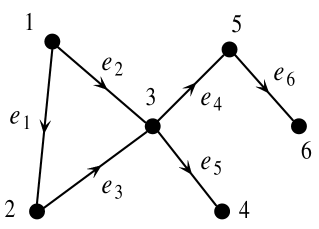
Figure 3: The input directed graph $G$

Now let $G=(V,E)$ be the directed graph in Figure 3, where $|V|=6$ and $|E\hskip 0.85355pt|=6$. We illustrate the domain reduction process by constructing the first labeled directed graph $\mathcal{G}_{1}$ in the sequence as follows. To simplify the presentation, we let $\mathbf{y}\in[8]^{6}$ (instead of $\xi:V\rightarrow[8]$) denote an assignment, where $y_{i}\in[8]$ denotes the value of vertex $i$ in Figure 3 for every $i\in[6]$.

First, let $\mathbf{y}\in[8]^{6}$ be any assignment with a nonzero weight: $A_{y_{i},y_{j}}>0$ for every edge $ij\in E$. Since $\mathbf{A}$ has the block structure $\mathcal{T}$, for every $ij\in E$, there exists a unique index $s\in[4]$ such that $y_{i}\in A_{s}$ and $y_{j}\in B_{s}$. This inspires us to introduce a new variable $x_{\ell}\in[4]$ for each edge $e_{\ell}\in E$, $\ell\in[6]$ (as shown in Figure 3). For every possible assignment of $\mathbf{x}=(x_{1},x_{2},\ldots,x_{6})\in[4]^{6}$, we use $Y[\mathbf{x}]$ to denote the set of all possible assignments $\mathbf{y}\in[8]^{6}$ such that for every $e_{\ell}=ij$, $y_{i}\in A_{x_{\ell}}$ and $y_{j}\in B_{x_{\ell}}$. Now we have

$$Z_{\mathbf{A}}(G)=\sum_{\mathbf{x}\in[4]^{6}}\hskip 2.27626pt\sum_{\mathbf{y}\in Y[\mathbf{x}]}\text{wt}(\mathbf{y}),\ \ \ \ \text{where $\text{wt}(\mathbf{y})=\prod_{ij\in E}A_{y_{i},y_{j}}$.}$$

Second, we further simplify the sum above by noticing that if $x_{2}\neq x_{3}$ in $\mathbf{x}$, then $Y[\mathbf{x}]$ must be empty because the two edges $e_{2}$ and $e_{3}$ share the same tail in $G$. In general, we only need to sum over the case when $x_{1}=x_{2}=x_{3}$ and $x_{4}=x_{5}$, since otherwise the set $Y[\mathbf{x}]$ is empty. As a result,

$$Z_{\mathbf{A}}(G)=\sum_{\begin{subarray}{c}x_{1}=x_{2}=x_{3}\\ x_{4}=x_{5}\\ x_{6}\end{subarray}}\hskip 2.27626pt\sum_{\mathbf{y}\in Y[\mathbf{x}]}\text{wt}(\mathbf{y}).$$

The advantage of introducing $x_{\ell}$, $\ell\in[6]$, is that, once $\mathbf{x}$ is fixed, one can always decompose $A_{y_{i},y_{j}}$ as a product $\alpha_{y_{i}}\cdot\beta_{y_{j}}$, for all $\mathbf{y}\in Y[\mathbf{x}]$ and all $ij\in E$, since $\mathbf{y}$ belonging to $Y[\mathbf{x}]$ guarantees that $(y_{i},y_{j})$ falls inside one of the four blocks of $\mathbf{A}$. This allows us to greatly simplify $\text{wt}(\mathbf{y})$: If $\mathbf{y}\in Y[\mathbf{x}]$, then

$$\text{wt}(\mathbf{y})=A_{y_{1},y_{3}}\cdot A_{y_{1},y_{2}}\cdot A_{y_{2},y_{3}}\cdot A_{y_{3},y_{4}}\cdot A_{y_{3},y_{5}}\cdot A_{y_{5},y_{6}}=\alpha_{y_{1}}\beta_{y_{3}}\alpha_{y_{1}}\beta_{y_{2}}\alpha_{y_{2}}\beta_{y_{3}}\alpha_{y_{3}}\beta_{y_{4}}\alpha_{y_{3}}\beta_{y_{5}}\alpha_{y_{5}}\beta_{y_{6}}.\vspace{0.07cm}$$

Also notice that $Y[\mathbf{x}]$, for any $\mathbf{x}$, is a direct product of subsets of $[8]$: $\mathbf{y}\in Y[\mathbf{x}]$ if and only if

$$y_{1}\in L_{1}=A_{x_{1}},\ y_{2}\in L_{2}=A_{x_{3}}\cap B_{x_{1}}=A_{x_{1}}\cap B_{x_{1}},\ y_{3}\in L_{3}=A_{x_{4}}\cap A_{x_{5}}\cap B_{x_{2}}\cap B_{x_{3}}=A_{x_{4}}\cap B_{x_{1}}$$

$$y_{4}\in L_{4}=B_{x_{4}},y_{5}\in L_{5}=A_{x_{6}}\cap B_{x_{4}},y_{6}\in L_{6}=B_{x_{6}}.\vspace{0.3cm}$$

As a result, $Z_{\mathbf{A}}(G)$ becomes

$$Z_{\mathbf{A}}(G)=\sum_{x_{1},x_{4},x_{6}}\hskip 2.84544pt\sum_{y_{i}\in L_{i},\hskip 1.42271pti\in[6]}\left((\alpha_{y_{1}})^{2}\alpha_{y_{2}}\beta_{y_{2}}\right)\cdot\left((\alpha_{y_{3}})^{2}(\beta_{y_{3}})^{2}\right)\cdot\beta_{y_{4}}\cdot(\alpha_{y_{5}}\beta_{y_{5}})\cdot\beta_{y_{6}}.$$ (1)

Finally we construct the following labeled directed graph $\mathcal{G}_{1}$ over domain $[4]$. There are three vertices $a,b$ and $c$, which correspond to $x_{1},x_{4}$ and $x_{6}$, respectively; and there are two directed edges $ab$ and $bc$. We construct the weights as follows. The vertex weight vector of $a$ is

$$w^{[a]}_{\ell}=\sum_{y_{1}\in A_{\ell},\hskip 2.27626pty_{2}\in A_{\ell}\cap B_{\ell}}(\alpha_{y_{1}})^{2}\cdot(\alpha_{y_{2}}\beta_{y_{2}}),\ \ \ \ \text{for every $\ell\in[4]$};$$

the vertex weights of $b$ and $c$ are the same:

$$w^{[b]}_{\ell}=w^{[c]}_{\ell}=\sum_{y\in B_{\ell}}\beta_{y},\ \ \ \ \text{for every $\ell\in[4]$.}$$

The edge weight matrix $\mathbf{C}^{[ab]}$ of $ab$ is

$$C^{[ab]}_{k,\ell}=\sum_{y_{3}\in B_{k}\cap A_{\ell}}(\alpha_{y_{3}})^{2}(\beta_{y_{3}})^{2},\ \ \ \ \text{for all $k,\ell\in[4]$;}$$

and the edge weight matrix $\mathbf{C}^{[bc]}$ of $bc$ is

$$C^{[bc]}_{k,\ell}=\sum_{y_{5}\in B_{k}\cap A_{\ell}}\alpha_{y_{5}}\beta_{y_{5}},\ \ \ \ \text{for all $k,\ell\in[4]$.}$$

Using (1) and the definition of $Z(\mathcal{G}_{1})$, it is easy to verify that $Z_{\mathbf{A}}(G)=Z(\mathcal{G}_{1})$ and thus, we reduced the domain size of the problem from $8$ (which is the number of rows and columns in $\mathbf{A}$), to $4$ (which is the number of blocks in $\mathbf{A}$). However, we also paid a high price. Two issues are worth pointing out here:

1. Unlike in $Z_{\mathbf{A}}(G)$, different edges in $\mathcal{G}_{1}$ have different edge weight matrices in general. For example, the matrices associated with $ab$ and $bc$ are clearly different, for general $\boldsymbol{\alpha}$ and $\boldsymbol{\beta}$. Actually, the set of matrices that may appear as an edge weight of $\mathcal{G}_{1}$, constructed from all possible directed graphs $G$ after one round of domain reduction, is infinite in general.

2. Unlike in $Z_{\mathbf{A}}(G)$, we have to introduce vertex weights in $\mathcal{G}_{1}$. Similarly, vertices may have different vertex weight vectors, and the set of vectors that may appear as a vertex weight of $\mathcal{G}_{1}$, constructed from all possible $G$ after one round of domain reduction, is infinite in general.

It is also worth noticing that even if the matrix $\mathbf{A}$ we start with is $\{0,1\}$, the edge and vertex weights of $\mathcal{G}_{1}$ immediately become rational right after the first round of domain reduction and we have to deal with rational weights afterwards. So $\{0,1\}$-matrices are not that special under this framework.

These two issues cause us a lot of trouble because we need to carry out the domain reduction process for several times, until the computation becomes trivial. However, the reduction process above crucially used the assumption that $\mathbf{A}$ is block-rank-$1$ (otherwise one cannot replace $A_{i,j}$ with $\alpha_{i}\cdot\beta_{j}$). Therefore, there is no way to continue this process if some edge weight matrix in $\mathcal{G}_{1}$ is not block-rank-1. To deal with this case, we show that if this happens for some $G$, then $Z_{\mathbf{A}}(\cdot)$ is #P-hard. Informally, we have

Theorem 1 (Informal).

For any $G$, if one of the edge matrices in $\mathcal{G}_{k}$ (constructed from $G$ after $k$ rounds of domain reductions), for some $k\geq 1$, is not block-rank-$1$, then $Z_{\mathbf{A}}(\cdot)$ is #P-hard.

The proof of Theorem 1 for $k=1$ is relatively straight forward, because every edge weight matrix in $G$ is $\mathbf{A}$. However, due of the two issues mentioned earlier, the edge weights and vertex weights of $\mathcal{G}_{1}$ are drawn from infinite sets in general, and even proving it for $k=2$ is highly non-trivial.

Even with Theorem 1 which essentially gives us a dichotomy theorem for all non-negative matrices, it is still unclear whether the dichotomy is decidable or not. The difficulty is that, to decide whether $Z_{\mathbf{A}}(\cdot)$ is in P or #P-hard, we need to check infinitely many matrices (all the edge weight matrices that appear in the domain reduction process, from all possible directed graphs $G$) and to see whether all of them are block-rank-$1$. To overcome this, we give an algebraic proof using properties of polynomials. We manage to show that it is not necessary to check these matrices one by one, but only need to check whether or not the entries of $\mathbf{A}$ satisfy finitely many polynomial constraints.

1.2 Proof Sketch

Without loss of generality, we assume that $\mathbf{A}$ is a nonnegative block-rank-$1$ matrix. To show that $Z_{\mathbf{A}}(\cdot)$ is either in P or #P-hard, we use the following two steps.

In the first step, we define from $\mathbf{A}$ a finite sequence of pairs:

$$({\mathfrak{X}}_{0},{\mathfrak{Y}}_{0}),({\mathfrak{X}}_{1},{\mathfrak{Y}}_{1}),\ldots,({\mathfrak{X}}_{h},{\mathfrak{Y}}_{h}),\ \ \ \ \text{for some $h:0\leq h<m$,}$$

where ${\mathfrak{X}}_{0}=\{\mathbf{1}\}$, ${\mathfrak{Y}}_{0}=\{\mathbf{A}\}$ and $\mathbf{1}$ denotes the $m$-dimensional all-$1$ vector. Each pair $({\mathfrak{X}}_{k},{\mathfrak{Y}}_{k})$, $k\in[h]$, is defined from $({\mathfrak{X}}_{k-1},{\mathfrak{Y}}_{k-1})$. Roughly speaking, ${\mathfrak{Y}}_{k}$ (resp. ${\mathfrak{X}}_{k}$) is the set of all edge matrices (resp. vertex vectors) that may appear in $\mathcal{G}_{k}$, after $k$ rounds of domain reductions. There also exist positive integers

$$m=m_{0}>m_{1}>\ldots>m_{h}\geq 1\vspace{-0.04cm}$$

such that every ${\mathfrak{Y}}_{k}$, $k\in[h]$, is a set of $m_{k}\times m_{k}$ non-negative matrices; and every ${\mathfrak{X}}_{k}$, $k\in[h]$, is a set of $m_{k}$-dimensional non-negative vectors. Although the sets ${\mathfrak{X}}_{k}$ and ${\mathfrak{Y}}_{k}$ are infinite in general (which is the reason why we used the word “define” instead of “construct”), the definition of $({\mathfrak{X}}_{k},{\mathfrak{Y}}_{k})$ guarantees the following two properties:

1. For each $k\in[h]$, all matrices in ${\mathfrak{Y}}_{k}$ share the same structure: $\forall\hskip 1.70709pt\mathbf{B},\mathbf{B}^{\prime}\in{\mathfrak{Y}}_{k}$, $B_{i,j}>0\hskip 1.42271pt\Leftrightarrow\hskip 1.42271ptB_{i,j}^{\prime}>0$;

2. Every matrix $\mathbf{B}$ in ${\mathfrak{Y}}_{h}$ is a permutation matrix.

The definition of $({\mathfrak{X}}_{k},{\mathfrak{Y}}_{k})$ from $({\mathfrak{X}}_{k-1},{\mathfrak{Y}}_{k-1})$ can be found in Appendix C. In Appendix F we prove that for every $k\in[h]$, if $\mathbf{B}\in{\mathfrak{Y}}_{k}$, then the problem of computing $Z_{\mathbf{B}}(\cdot)$ is polynomial-time reducible to the computation of $Z_{\mathbf{A}}(\cdot)$. From this, we can obtain the hardness part of our dichotomy theorem: If for some $k\in[h]$, there exists a matrix $\mathbf{B}\in{\mathfrak{Y}}_{k}$ such that $\mathbf{B}$ is not block-rank-1, then $Z_{\mathbf{A}}(\cdot)$ is #P-hard.

Now we assume that all matrices in ${\mathfrak{Y}}_{k}$, $k\in[h]$, are block-rank-1. To finish the proof we only need to show that if this is true, then $Z_{\mathbf{A}}(\cdot)$ is indeed in P. To this end, we use the domain reduction process to construct a sequence of labeled directed graphs $\mathcal{G}_{1},\ldots,\mathcal{G}_{h}$ such that

1. $Z(\mathcal{G}_{1})=Z_{\mathbf{A}}(G)$ and $Z(\mathcal{G}_{k+1})=Z(\mathcal{G}_{k})$ for all $k:1\leq k<h$; and

2. For every $k\in[h]$, we have $\mathbf{A}^{[e]}\in{\mathfrak{Y}}_{k}$ for all edges $e$ in $\mathcal{G}_{k}$ and $\mathbf{w}^{[v]}\in{\mathfrak{X}}_{k}$ for all vertices $v$ in $\mathcal{G}_{k}$.

This sequence can be constructed in polynomial time, because the construction of ${\cal G}_{k+1}$ from ${\cal G}_{k}$ can be done very efficiently as described in Section 1.1, and also because the number of graphs in the sequence is at most $m$. By the two properties above, we have $Z_{\mathbf{A}}(G)=Z(\mathcal{G}_{h})$; and every edge weight matrix $\mathbf{A}^{[e]}$ in $\mathcal{G}_{h}$ is a permutation matrix. As a result, we can compute $Z_{\mathbf{A}}(G)$ in polynomial time since $Z(\mathcal{G}_{h})$ can be computed efficiently.

This finishes the proof of our dichotomy theorem: given any non-negative matrix $\mathbf{A}$, the problem of computing $Z_{\mathbf{A}}(\cdot)$ is either in polynomial time or #P-hard. Moreover, to decide which case it is, we only need to check whether the matrices in ${\mathfrak{Y}}_{k}$, $k\in[h]$, satisfy the following condition:

The Block-Rank-1 Condition: Every matrix $\mathbf{B}\in{\mathfrak{Y}}_{k}$, $k\in[h]$, is block-rank-$1$.

However, as mentioned earlier, all the sets ${\mathfrak{Y}}_{k}$, $k\in[h]$, are infinite in general, so one cannot check the matrices one by one. Instead, we express the block-rank-$1$ condition as a finite collection of polynomial constraints over ${\mathfrak{Y}}_{k}$. The way $({\mathfrak{X}}_{k},{\mathfrak{Y}}_{k})$ is defined from $({\mathfrak{X}}_{k-1},{\mathfrak{Y}}_{k-1})$ allows us to prove that, to check whether every matrix in ${\mathfrak{Y}}_{k}$ (or every vector in ${\mathfrak{X}}_{k}$) satisfies a certain polynomial constraint, one only needs to check a finitely many polynomial constraints for $({\mathfrak{X}}_{k-1},{\mathfrak{Y}}_{k-1})$. Therefore, to check whether ${\mathfrak{Y}}_{k}$, $k\in[h]$, satisfies the block-rank-$1$ condition we only need to check a finitely many polynomial constraints for $({\mathfrak{X}}_{0},{\mathfrak{Y}}_{0})$. Since ${\mathfrak{X}}_{0}=\{\mathbf{1}\}$ and ${\mathfrak{Y}}_{0}=\{\mathbf{A}\}$ are both finite, this can be done in a finite number of steps.

2 Preliminaries

We say $\mathcal{G}=(G,\mathcal{V},\mathcal{E})$ is a labeled directed graph over $[m]=\{1,\ldots,m\}$ for some positive integer $m$, if

1. $G=(V,E)$ is a directed graph (which may have parallel edges but no self-loops);

2. Every vertex $v\in V$ is labeled with an $m$-dimensional non-negative vector $\mathcal{V}(v)\in\mathbb{R}_{+}^{m}$ as its
   vertex weight; and

3. Every edge $uv\in E$ is labeled with an $m\times m$ (not necessarily symmetric) non-negative matrix
   $\mathcal{E}(uv)\in\mathbb{R}_{+}^{m\times m}$ as its edge weight.

Let $\mathcal{G}=(G,\mathcal{V},\mathcal{E})$ be a labeled directed graph, where $G=(V,E)$. For each $v\in V$, we use $\mathbf{w}^{[v]}=\mathcal{V}(v)$ to denote its vertex weight vector; and for each $uv\in E$, we use $\mathbf{C}^{[uv]}=\mathcal{E}(uv)$ to denote its edge weight matrix. Then we define $Z(\mathcal{G})$ as follows:

$$Z(\mathcal{G})=\sum_{\xi:V\rightarrow[m]}\text{wt}(\mathcal{G},\xi),\ \ \ \ \text{where \hskip 2.27626pt$\text{wt}(\mathcal{G},\xi)=\prod_{v\in V}\hskip 1.42271ptw^{[v]}_{\xi(v)}\hskip 1.42271pt\prod_{uv\in E}C^{[uv]}_{\xi(u),\hskip 1.42271pt\xi(v)}$}$$

denotes the weight of the assignment $\xi$.

Let $\mathbf{C}$ be an $m\times m$ non-negative matrix. We are interested in the complexity of $Z_{\mathbf{C}}(\cdot)$:

$$Z_{\mathbf{C}}(G)=Z(\mathcal{G}),\ \ \ \ \ \text{for any directed graph $G=(V,E)$,}$$

where $\mathcal{G}=(G,\mathcal{V},\mathcal{E})$ is the labeled directed graph with $\mathcal{V}(v)=\mathbf{1}\in\mathbb{R}_{+}^{m}$ for all $v\in V$ and $\mathcal{E}(uv)=\mathbf{C}$ for all edges $uv\in E$.

Definition 1 (Pattern and block pattern).

We say $\mathcal{P}$ is an $m\times m$ pattern if $\mathcal{P}\subseteq[m]\times[m]$. $\mathcal{P}$ is said to be trivial if $\mathcal{P}=\emptyset$. A non-negative $m\times m$ matrix $\mathbf{C}$ is of pattern $\mathcal{P}$, if for all $i,j\in[m]$, we have $C_{i,j}$ $>0$ if and only if $(i,j)\in\mathcal{P}$. $\mathbf{C}$ is also called a $\mathcal{P}$-matrix. We say $\mathcal{T}$ is an $m\times m$ block pattern if

1. $\mathcal{T}=\big{\{}(A_{1},B_{1}),\ldots,(A_{r},B_{r})\big{\}}$ for some $r\geq 0$;

2. $A_{i}\subseteq[m]$, $A_{i}\neq\emptyset$, $B_{i}\subseteq[m]$ and $B_{i}\neq\emptyset$ for all $i\in[r]$; and

3. $A_{i}\cap A_{j}=B_{i}\cap B_{j}=\emptyset$, for all $i\neq j\in[r]$.

$\mathcal{T}$ is said to be trivial if $\mathcal{T}=\emptyset$. A block pattern $\mathcal{T}$ naturally defines a pattern $\mathcal{P}$, where

$$\mathcal{P}=\big{\{}\hskip 0.85355pt(i,j)\hskip 2.27626pt\big{|}\hskip 1.9919pt\exists\hskip 1.70709ptk\in[r]\ \text{such that \hskip 1.13791pt$i\in A_{k}$ and $j\in B_{k}$}\big{\}}.$$

We also say $\mathcal{P}$ is consistent with $\mathcal{T}$. Finally, we say a non-negative $m\times m$ matrix $\mathbf{C}$ is of block pattern $\mathcal{T}$, if $\mathbf{C}$ is of pattern $\mathcal{P}$ defined by $\mathcal{T}$. $\mathbf{C}$ is also called a $\mathcal{T}$-matrix.

Definition 2.

We say an $m\times m$ non-negative matrix $\mathbf{C}$ is block-rank-$1$ if

1. Either $\mathbf{C}=\mathbf{0}$ is the zero matrix (and is of block pattern $\mathcal{T}=\emptyset$); or

2. $\mathbf{C}$ is of block pattern $\mathcal{T}$, for some $m\times m$ block pattern $\mathcal{T}=\{(A_{1},B_{1}),\ldots,(A_{r},B_{r})\}$ with $r\geq 1$;
   and for every $k\in[r]$, the sub-matrix of $\mathbf{C}$ induced by $A_{k}$ and $B_{k}$ is (exactly) rank $1$.

Let $\mathbf{C}$ be a non-negative block-rank-$1$ matrix of block pattern $\mathcal{T}$. Then there exists a unique pair $(\boldsymbol{\alpha},\boldsymbol{\beta})$ of non-negative $m$-dimensional vectors such that

1. For every $i\in[m]$, $\alpha_{i}>0\hskip 1.13791pt\Longleftrightarrow\hskip 1.13791pti\in\bigcup_{k\in[r]}A_{k}$; and $\beta_{i}>0\hskip 1.13791pt\Longleftrightarrow\hskip 1.13791pti\in\bigcup_{k\in[r]}B_{k}$;

2. $C_{i,j}=\alpha_{i}\cdot\beta_{j}$ for all $i,j\in[m]$ such that $C_{i,j}>0$; and

3. $\sum_{j\in A_{i}}\alpha_{j}=1$, for all $i\in[r]$.

The pair $(\boldsymbol{\alpha},\boldsymbol{\beta})$ is called the (vector) representation of $\mathbf{C}$. Note that we have $\boldsymbol{\alpha}=\boldsymbol{\beta}=\mathbf{0}$ when $\mathbf{C}=\mathbf{0}$.

It is clear that $\mathcal{T}$ and $(\boldsymbol{\alpha},\boldsymbol{\beta})$ together uniquely determine a non-negative block-rank-$1$ matrix.

The following lemma concerns the complexity of $Z_{\mathbf{C}}(\cdot)$. The proof can be found in Appendix B.

Lemma 1.

If $\mathbf{C}$ is not block-rank-$1$, then $Z_{\mathbf{C}}(\cdot)$ is #P-hard.

Let $\mathcal{T}$ be an $m\times m$ non-trivial block pattern where $\mathcal{T}=\{(A_{1},B_{1}),\ldots,(A_{r},B_{r})\}$ for some $r\geq 1$. It defines the following $r\times r$ pattern $\mathcal{P}=\text{{gen}}(\mathcal{T})$: For all $i,j\in[r]$, $(i,j)\in\mathcal{P}$ if and only if $B_{i}\cap A_{j}\neq\emptyset.$

We also define $\text{{gen-block}}(\mathcal{T})$ as follows:

1. If $\mathcal{P}=\text{{gen}}(\mathcal{T})$ is consistent with a block pattern, denoted by $\mathcal{T}^{\prime}$, then $\text{{gen-block}}(\mathcal{T})=\mathcal{T}^{\prime}$;

2. Otherwise, we set $\text{{gen-block}}(\mathcal{T})=\text{\rm{\emph{false}}}$.

We note that $\mathcal{P}=\text{{gen}}(\mathcal{T})$ could be trivial even if $\mathcal{T}$ is non-trivial.

Next, we introduce a generalized version of $Z_{\mathbf{C}}(\cdot)$. Let $m\geq 1$ and $(\mathfrak{P},\mathfrak{Q})$ be a pair in which

1. $\mathfrak{P}$ is a finite and nonempty set of non-negative $m$-dimensional vectors with $\mathbf{1}\in\mathfrak{P}$; and

2. $\mathfrak{Q}$ is a finite and nonempty set of $m\times m$ non-negative matrices.

We then use $Z(\cdot)$ to define the function $Z_{\mathfrak{P},\mathfrak{Q}}(\cdot)$ as follows:

$$Z_{\mathfrak{P},\mathfrak{Q}}(\mathcal{G})=Z(\mathcal{G}),$$

where $\mathcal{G}=(G,\mathcal{V},\mathcal{E})$ is a labeled directed graph with $\mathcal{V}(v)\in\mathfrak{P}$ for any vertex $v\in V(G)$; and $\mathcal{E}(uv)\in\mathfrak{Q}$ for any edge $uv\in E(G)$. As an example, $Z_{\mathbf{C}}(\cdot)$ is exactly $Z_{\mathfrak{P},\mathfrak{Q}}(\cdot)$ with $\mathfrak{P}=\{\mathbf{1}\}$ and $\mathfrak{Q}=\{\mathbf{C}\}$.

Finally, let $m\geq 1$ and $({\mathfrak{X}},{\mathfrak{Y}})$ and $({\mathfrak{X}}^{\prime},{\mathfrak{Y}}^{\prime})$ be two pairs such that:

1. ${\mathfrak{X}}$ and ${\mathfrak{X}}^{\prime}$ are two nonempty (and possibly infinite) sets of non-negative $m$-dimensional
   vectors with $\mathbf{1}\in{\mathfrak{X}}$ and $\mathbf{1}\in{\mathfrak{X}}^{\prime}$; and

2. ${\mathfrak{Y}}$ and ${\mathfrak{Y}}^{\prime}$ are two nonempty (and possibly infinite) sets of non-negative $m\times m$ matrices.

Definition 3 (Reduction).

We say $({\mathfrak{X}}^{\prime},{\mathfrak{Y}}^{\prime})$ is polynomial-time reducible to $({\mathfrak{X}},{\mathfrak{Y}})$ if for every finite and nonempty subset $\mathfrak{P}^{\prime}\subseteq{\mathfrak{X}}^{\prime}$ with $\mathbf{1}\in\mathfrak{P}^{\prime}$ and every finite and nonempty subset $\mathfrak{Q}^{\prime}\subseteq{\mathfrak{Y}}^{\prime}$, there exist a finite and nonempty subset $\mathfrak{P}\subseteq{\mathfrak{X}}$ with $\mathbf{1}\in\mathfrak{P}$ and a finite and nonempty subset $\mathfrak{Q}\subseteq{\mathfrak{Y}}$, such that $Z_{\mathfrak{P}^{\prime},\mathfrak{Q}^{\prime}}(\cdot)$ is polynomial-time reducible to $Z_{\mathfrak{P},\mathfrak{Q}}(\cdot)$.

3 Main Theorems

We prove a complexity dichotomy theorem for all counting problems $Z_{\mathbf{C}}(\cdot)$ where $\mathbf{C}$ is any non-negative matrix. Actually, our main theorem is more general.

Definition 4.

Let $\mathcal{P}$ be an $m\times m$ pattern. An $m$-dimensional non-negative vector $\mathbf{w}$ is said to be

• positive: $w_{i}>0$ for all $i\in[m]$; and

• $\mathcal{P}$-weakly positive: for all $i\in[m]$, $w_{i}>0$ if and only if $(i,i)\in\mathcal{P}$.

We call $({\mathfrak{X}},{\mathfrak{Y}})$ a $\mathcal{P}$-pair if

1. ${\mathfrak{X}}$ is a nonempty (and possibly infinite) set of positive and $\mathcal{P}$-weakly positive vectors with $\mathbf{1}\in{\mathfrak{X}}$;

2. ${\mathfrak{Y}}$ is a nonempty (and possibly infinite) set of $m\times m$ (non-negative) $\mathcal{P}$-matrices.

We say it is a finite $\mathcal{P}$-pair if both sets are finite. We normally use $(\mathfrak{P},\mathfrak{Q})$ to denote a finite $\mathcal{P}$-pair.

Similarly, for any $m\times m$ block pattern $\mathcal{T}$, we can define $\mathcal{T}$-weakly positive vectors as well as $\mathcal{T}$-pairs by replacing the $\mathcal{P}$ above with the pattern defined by $\mathcal{T}$.

We prove the following complexity dichotomy theorem:

Theorem 2 (Complexity Dichotomy).

Let $\mathcal{P}$ be an $m\times m$ pattern for some $m\geq 1$, then for any finite $\mathcal{P}$-pair $(\mathfrak{P},\mathfrak{Q})$, the problem of computing $Z_{\mathfrak{P},\mathfrak{Q}}(\cdot)$ is either in polynomial time or #P-hard.

Clearly, it gives us a dichotomy for the special case of $Z_{\mathbf{C}}(\cdot)$ when $\mathfrak{P}=\{\mathbf{1}\}$ and $\mathfrak{Q}=\{\mathbf{C}\}$. Moreover, we show that for the special case when $\mathfrak{P}=\{\mathbf{1}\}$, we can decide in a finite number of steps whether $Z_{\mathfrak{P},\mathfrak{Q}}$ is in polynomial time or #P-hard. In particular, it implies that the dichotomy for $Z_{\mathbf{C}}(\cdot)$ is decidable.

Theorem 3 (Decidability).

Given any positive integer $m\geq 1$, an $m\times m$ pattern $\mathcal{P}$, and a finite $\mathcal{P}$-pair $(\mathfrak{P},\mathfrak{Q})$ with $\mathfrak{P}=\{\mathbf{1}\}$, the problem of whether $Z_{\mathfrak{P},\mathfrak{Q}}(\cdot)$ is in polynomial time or #P-hard is decidable.

We prove Theorem 2 and 3 in the rest of the section. The lemmas (Lemma 2, 3, and 4) used in the proof will be proved in the appendix.

3.1 Defining New Pairs: gen-pair $({\mathfrak{X}},{\mathfrak{Y}})$

Before proving Theorem 2, we state a key lemma which will be proved in Appendix C and Appendix F.

Let $({\mathfrak{X}},{\mathfrak{Y}})$ be a (possibly infinite) $\mathcal{T}$-pair, for some non-trivial $m\times m$ block pattern $\mathcal{T}$. Also assume that every matrix in ${\mathfrak{Y}}$ is block-rank-$1$. Then in Appendix C, we introduce an operation gen-pair over $({\mathfrak{X}},{\mathfrak{Y}})$, which defines a new (and possibly infinite) pair $({\mathfrak{X}}^{\prime},{\mathfrak{Y}}^{\prime})=\text{{gen-pair}}({\mathfrak{X}},{\mathfrak{Y}}).$

Definition 5.

A set $S$ of non-negative $m$-dimensional vectors, for some $m\geq 1$, is closed if $\mathbf{w}_{1}\circ\mathbf{w}_{2}\in S$ for all vectors $\mathbf{w}_{1},\mathbf{w}_{2}\in S$, where we let $\circ$ denote the Hadamard product of two vectors: $\mathbf{w}_{1}\circ\mathbf{w}_{2}$ is the $m$-dimensional vector whose $i$th entry is $w_{1,i}\cdot w_{2,i}$ for all $i\in[m]$.

In Appendix F, we prove the following lemma.

Lemma 2.

Let $({\mathfrak{X}},{\mathfrak{Y}})$ be a $\mathcal{T}$-pair, for some non-trivial block pattern $\mathcal{T}$. Suppose every matrix in ${\mathfrak{Y}}$ is block-rank-$1$, then $({\mathfrak{X}}^{\prime},{\mathfrak{Y}}^{\prime})=\text{\emph{{gen-pair}}}({\mathfrak{X}},{\mathfrak{Y}})$ is a $\mathcal{P}^{\prime}$-pair, where $\mathcal{P}^{\prime}=\text{\emph{{gen}}}(\mathcal{T})$. The new vector set ${\mathfrak{X}}^{\prime}$ is closed and $({\mathfrak{X}}^{\prime},{\mathfrak{Y}}^{\prime})$ is polynomial-time reducible to $({\mathfrak{X}},{\mathfrak{Y}})$.

3.2 Proof of Theorem 2

Let $(\mathfrak{P},\mathfrak{Q})$ be a finite $\mathcal{P}$-pair, where $\mathcal{P}$ is an $m\times m$ pattern.

We assume $Z_{\mathfrak{P},\mathfrak{Q}}(\cdot)$ is not #P-hard, and we only need to show that $Z_{\mathfrak{P},\mathfrak{Q}}(\cdot)$ is in polynomial time.

By Lemma 1, there must be a block pattern $\mathcal{T}$ consistent with $\mathcal{P}$ and all the matrices in $\mathfrak{Q}$ are block- rank-$1$ since otherwise $Z_{\mathfrak{P},\mathfrak{Q}}(\cdot)$ is #P-hard, which contradicts the assumption. Therefore, we have

• $(\mathfrak{P},\mathfrak{Q})$ is a finite $\mathcal{T}$-pair for some $m\times m$ block pattern $\mathcal{T}$; and
  Every matrix in $\mathfrak{Q}$ is block-rank-$1$.

For convenience, we rename $(\mathfrak{P},\mathfrak{Q})$ to be $({\mathfrak{X}}_{0},{\mathfrak{Y}}_{0})$ and rename $m$ and $\mathcal{T}$ to be $m_{0}$ and $\mathcal{T}_{0}$, respectively.

Now we define a finite sequence of pairs using the gen-pair operation, starting with $({\mathfrak{X}}_{0},{\mathfrak{Y}}_{0})$.

First, if $|A_{i}|=|B_{i}|=1$ for all $i$, i.e., every set $A_{i}$ and $B_{i}$ in $\mathcal{T}_{0}$ is a singleton, then the sequence has only one pair $({\mathfrak{X}}_{0},{\mathfrak{Y}}_{0})$, and the definition of this sequence is complete. Note that this also includes the special case when $\mathcal{T}_{0}=\emptyset$ and ${\mathfrak{Y}}_{0}=\{\mathbf{0}\}$.

Otherwise, in Step $1$, we define a new $\mathcal{P}_{1}$-pair $({\mathfrak{X}}_{1},{\mathfrak{Y}}_{1})$ using gen-pair:

$$({\mathfrak{X}}_{1},{\mathfrak{Y}}_{1})=\text{{gen-pair}}({\mathfrak{X}}_{0},{\mathfrak{Y}}_{0}),\ \ \ \ \ \text{where $\mathcal{P}_{1}=\text{{gen}}(\mathcal{T}_{0})$.}\vspace{-0.03cm}$$

By Lemma 2 $({\mathfrak{X}}_{1},{\mathfrak{Y}}_{1})$ is polynomial-time reducible to $({\mathfrak{X}}_{0},{\mathfrak{Y}}_{0})$. This implies that $\mathcal{P}_{1}$ must be consistent with a block pattern, denoted by $\mathcal{T}_{1}$, and every matrix in ${\mathfrak{Y}}_{1}$ is block-rank-$1$. (Otherwise, assume $\mathbf{D}\in{\mathfrak{Y}}_{1}$ is not block-rank-1, then by Lemma 1, $Z_{\mathfrak{P}_{1},\mathfrak{Q}_{1}}(\cdot)$ is #P-hard, where $\mathfrak{P}_{1}=\{\mathbf{1}\}$ and $\mathfrak{Q}_{1}=\{\mathbf{D}\}$. It follows from Lemma 2 that there exists a finite pair $(\mathfrak{P}_{0},\mathfrak{Q}_{0})$ where $\mathfrak{P}_{0}\subseteq{\mathfrak{X}}_{0}$ and $\mathfrak{Q}_{0}\subseteq{\mathfrak{Y}}_{0}$, such that $Z_{\mathfrak{P}_{1},\mathfrak{Q}_{1}}(\cdot)$ is polynomial-time reducible to $Z_{\mathfrak{P}_{0},\mathfrak{Q}_{0}}(\cdot)$. On the other hand, it is clear that $Z_{\mathfrak{P}_{0},\mathfrak{Q}_{0}}(\cdot)$ is reducible to $Z_{{\mathfrak{X}}_{0},{\mathfrak{Y}}_{0}}(\cdot)$ and thus, the latter is also #P-hard, which contradicts our assumption.) As a result, we have

• $\mathcal{T}_{1}=\text{{gen-block}}(\mathcal{T}_{0})$ is an $m_{1}\times m_{1}$ block pattern, where $m_{1}$ is the number of pairs in $\mathcal{T}_{0}$;
  $({\mathfrak{X}}_{1},{\mathfrak{Y}}_{1})=\text{{gen-pair}}({\mathfrak{X}}_{0},{\mathfrak{Y}}_{0})$ is a $\mathcal{T}_{1}$-pair, and every matrix in ${\mathfrak{Y}}_{1}$ is block-rank-$1$.

We also have $m_{0}>m_{1}$ since at least one of the sets in $\mathcal{T}_{0}$ is not a singleton.

We remark that both sets ${\mathfrak{X}}_{1}$ and ${\mathfrak{Y}}_{1}$ are generally infinite, so one can not check the matrices in ${\mathfrak{Y}}_{1}$ for the block-rank-$1$ property one by one. It does not matter right now because we are only proving the dichotomy theorem. However, it will become a serious problem later when we show that the dichotomy is decidable. We have to show that the block-rank-$1$ property can be verified in a finite number of steps.

We then repeat the process above. After $\ell\geq 1$ steps, we get a sequence of $\ell+1$ pairs:

$$({\mathfrak{X}}_{0},{\mathfrak{Y}}_{0}),({\mathfrak{X}}_{1},{\mathfrak{Y}}_{1}),\ldots,({\mathfrak{X}}_{\ell},{\mathfrak{Y}}_{\ell}),\vspace{-0.01cm}$$

and $\ell+1$ block patterns $\mathcal{T}_{0},\mathcal{T}_{1},\ldots,\mathcal{T}_{\ell}$ such that

• For every $i\in[\ell]$, $\mathcal{T}_{i}=\text{{gen-block}}(\mathcal{T}_{i-1})$;
  For every $i\in[\ell]$, $({\mathfrak{X}}_{i},{\mathfrak{Y}}_{i})=\text{{gen-pair}}({\mathfrak{X}}_{i-1},{\mathfrak{Y}}_{i-1})$ is a $\mathcal{T}_{i}$-pair; and
  For every $i\in[0:\ell]$, all the matrices in ${\mathfrak{Y}}_{i}$ are block-rank-$1$.

We have two cases. If every set in $\mathcal{T}_{\ell}$ is a singleton (including the case when $\mathcal{T}_{\ell}=\emptyset$ and ${\mathfrak{Y}}_{\ell}=\{\mathbf{0}\}$), then the sequence has only $\ell+1$ pairs and the definition of the sequence is complete. Otherwise in Step $\ell+1$ we apply the gen-pair operation again to define a new pair $({\mathfrak{X}}_{\ell+1},{\mathfrak{Y}}_{\ell+1})$ from $({\mathfrak{X}}_{\ell},{\mathfrak{Y}}_{\ell})$.

Finally, assuming $Z_{\mathfrak{P},\mathfrak{Q}}(\cdot)$ is not #P-hard, we get a sequence of $h+1$ pairs

$$({\mathfrak{X}}_{0},{\mathfrak{Y}}_{0}),({\mathfrak{X}}_{1},{\mathfrak{Y}}_{1}),\ldots,({\mathfrak{X}}_{h},{\mathfrak{Y}}_{h}),\ \ \ \ \ \text{for some $h\geq 0$,}\vspace{-0.01cm}$$

together with $h+1$ positive integers $m_{0}>\ldots>m_{h}\geq 1$ and $h+1$ block patterns $\mathcal{T}_{0},\ldots,\mathcal{T}_{h}$ such that

• For every $i\in[0:h]$, $\mathcal{T}_{i}$ is an $m_{i}\times m_{i}$ block pattern;
  For every $i\in[h]$, $\mathcal{T}_{i}=\text{{gen-block}}(\mathcal{T}_{i-1})$;
  Either $\mathcal{T}_{h}=\emptyset$ is trivial or every set in $\mathcal{T}_{h}$ is a singleton;
  For every $i\in[h]$, $({\mathfrak{X}}_{i},{\mathfrak{Y}}_{i})=\text{{gen-pair}}({\mathfrak{X}}_{i-1},{\mathfrak{Y}}_{i-1})$ is a $\mathcal{T}_{i}$-pair; and
  For every $i\in[0:h]$, all the matrices in ${\mathfrak{Y}}_{i}$ are block-rank-$1$.

Because $m_{0}>\ldots>m_{h}\geq 1$, we also have $h<m_{0}=m$.

3.2.1 Dichotomy

Now we know that if $Z_{\mathfrak{P},\mathfrak{Q}}(\cdot)$ is not #P-hard, then there is a sequence of $h+1$ pairs for some $h:0\leq h$ $<m$, which satisfies condition (R). To complete the dichotomy theorem, we show in Appendix D that

Lemma 3 (Tractability).

Given any block pattern $\mathcal{T}$ and a finite $\mathcal{T}$-pair $(\mathfrak{P},\mathfrak{Q})$, let $({\mathfrak{X}}_{0},{\mathfrak{Y}}_{0}),\ldots,({\mathfrak{X}}_{h},{\mathfrak{Y}}_{h})$ be a sequence of pairs defined as above, with $({\mathfrak{X}}_{0},{\mathfrak{Y}}_{0})=(\mathfrak{P},\mathfrak{Q})$. Suppose it satisfies condition (R), then $Z_{\mathfrak{P},\mathfrak{Q}}(\cdot)$ is computable in polynomial time.

This finishes the proof of Theorem 2.

3.3 Proof of Theorem 3

Next, we show that for the special case when ${\mathfrak{X}}_{0}=\mathfrak{P}=\{\mathbf{1}\}$, the dichotomy theorem is decidable.

First, the condition (R₀) can be checked easily since there are only finitely many matrices in ${\mathfrak{Y}}_{0}$.

Assume after $\ell:0\leq\ell<m$ steps, we get a sequence of $\ell+1$ pairs: $({\mathfrak{X}}_{0},{\mathfrak{Y}}_{0}),({\mathfrak{X}}_{1},{\mathfrak{Y}}_{1}),\ldots,({\mathfrak{X}}_{\ell},{\mathfrak{Y}}_{\ell}),$ together with $\ell+1$ block patterns $\mathcal{T}_{0},\ldots,\mathcal{T}_{\ell}$. Moreover, we know that they satisfy (R_ℓ). If every set in $\mathcal{T}_{\ell}$ is a singleton (including the case when $\mathcal{T}_{\ell}=\emptyset$), then we are done because by Lemma 3, the problem is in polynomial time. Otherwise, to prove Theorem 3, we need a finite-time algorithm to check whether every matrix in the new $\mathcal{P}$-pair $({\mathfrak{X}}_{\ell+1},{\mathfrak{Y}}_{\ell+1})=\text{{gen-pair}}({\mathfrak{X}}_{\ell},{\mathfrak{Y}}_{\ell})$, where $\mathcal{P}=\texttt{gen}(\mathcal{T}_{\ell})$, is block-rank-$1$ or not. We refer to this property as the rank property for ${\mathfrak{Y}}_{\ell+1}$.

We prove the following lemma in Appendix G. Theorem 3 then follows.

Lemma 4.

Given any block pattern $\mathcal{T}$ and a finite $\mathcal{T}$-pair $({\mathfrak{X}}_{0},{\mathfrak{Y}}_{0})$ with ${\mathfrak{X}}_{0}=\{\mathbf{1}\}$, let $({\mathfrak{X}}_{0},{\mathfrak{Y}}_{0}),\ldots,({\mathfrak{X}}_{\ell},{\mathfrak{Y}}_{\ell})$ be a sequence of pairs defined as above. Suppose it satisfies condition (R_ℓ). Then the rank property for ${\mathfrak{Y}}_{\ell+1}$ can be checked in a finite number of steps.

Appendix A Figures

Figure 1: A directed graph $H$ such that $Z_{H}(\cdot)$ is tractable

$$\mathbf{A}=\begin{pmatrix}\hskip 2.27626ptA_{1,1}&&A_{1,3}\\ \hskip 2.27626ptA_{2,1}&&A_{2,3}\\ &&&&A_{3,5}&&A_{3,7}\\ &&&&A_{4,5}&&A_{4,7}\\ &A_{5,2}&&A_{5,4}\\ &A_{6,2}&&A_{6,4}\\ &&&&&A_{7,6}&&A_{7,8}\hskip 3.41418pt\\ &&&&&A_{8,6}&&A_{8,8}\hskip 3.41418pt\end{pmatrix}$$

Figure 2: The $8\times 8$ block-rank-$1$ matrix $\mathbf{A}$

Appendix B Proof of Lemma 1

Bulatov and Grohe showed that for any $m\times m$ non-negative symmetric matrix $\mathbf{D}$, $Z_{\mathbf{D}}(\cdot)$ is #P-hard if $\mathbf{D}$ is not block-rank-$1$. Note that when $\mathbf{D}$ is symmetric, the directions of the edges in $G$ do not affect the value of $Z_{\mathbf{D}}(G)$, so we can always assume that $G$ is an undirected graph.

We prove Lemma 1 by giving a reduction from the symmetric case.

Let $\mathbf{C}$ be an $m\times m$ non-negative matrix, which is not block-rank-$1$. Without loss of generality, we may assume that $\mathbf{C}_{1},\mathbf{C}_{2}$, the first and the second row vectors of $\mathbf{C}$, satisfy $\mathbf{C}_{1}\cdot\mathbf{C}_{2}>0$; but $\mathbf{C}_{1}$ and $\mathbf{C}_{2}$ are not linearly dependent. Let $\mathbf{D}$ denote the following symmetric matrix:

$$D_{i,j}=\mathbf{C}_{i}\cdot\mathbf{C}_{j},\ \ \ \ \ \text{for all $i,j\in[m]$}.$$

By the assumption, we have $D_{1,1},D_{1,2},D_{2,1},D_{2,2}>0$ but $D_{1,1}D_{2,2}>D_{1,2}D_{2,1}$. It then follows from the result of Bulatov and Grohe that $Z_{\mathbf{D}}(\cdot)$ is #P-hard to compute.

Now we prove the #P-hardness of $Z_{\mathbf{C}}(\cdot)$ by showing a reduction from $Z_{\mathbf{D}}(\cdot)$. Let $G=(V,E)$ be an input undirected graph of $Z_{\mathbf{D}}(\cdot)$. We construct a directed graph $G^{\prime}=(V^{\prime},E^{\prime})$ in which

$$V^{\prime}=V\cup\big{\{}\hskip 1.13791ptw_{e}:e\in E\hskip 1.13791pt\big{\}}\ \ \ \ \text{and}\ \ \ \ E^{\prime}=\big{\{}\hskip 1.13791ptuw_{e},vw_{e}:e=uv\in E\hskip 1.13791pt\big{\}}.$$

By the definition of $Z_{\mathbf{C}}(\cdot)$ and $Z_{\mathbf{D}}(\cdot)$, it is easy to verify that

$$Z_{\mathbf{C}}(G^{\prime})=Z_{\mathbf{D}}(G),\ \ \ \ \ \text{for any undirected graph $G$.}\vspace{-0.05cm}$$

As a result, $Z_{\mathbf{D}}(\cdot)$ is polynomial-time reducible to $Z_{\mathbf{C}}(\cdot)$, and the latter is also #P-hard.

Appendix C Definition of the gen-pair Operation

In this section, we define the operation gen-pair.

Let $\mathcal{T}=\{\hskip 0.28436pt(A_{1},B_{1}),\ldots,(A_{r},B_{r})\hskip 0.28436pt\}$ be a non-trivial $m\times m$ block pattern with $r\geq 1$. We use $\text{diag}(\mathcal{T})$ to denote the set of all $i\in[m]$ such that $i\in A_{k}$ and $i\in B_{k}$ for some $k\in[r]$. In this section, we always assume that $({\mathfrak{X}},{\mathfrak{Y}})$ is a $\mathcal{T}$-pair such that every matrix in ${\mathfrak{Y}}$ is block-rank-$1$. This means that

1. All matrices in ${\mathfrak{Y}}$ are block-rank-$1$ and are of the same block pattern $\mathcal{T}$;

2. $\mathbf{1}\in{\mathfrak{X}}$ and every vector $\mathbf{w}\in{\mathfrak{X}}$ is either

   1. positive: $w_{i}>0$ for all $i\in[m]$; or

   2. $\mathcal{T}$-weakly positive: $w_{i}>0$ if and only if $i\in\text{diag}(\mathcal{T})$.

Given such a pair $({\mathfrak{X}},{\mathfrak{Y}})$, gen-pair defines a new $\mathcal{P}$-pair

$$({\mathfrak{X}}^{\prime},{\mathfrak{Y}}^{\prime})=\texttt{gen-pair}({\mathfrak{X}},{\mathfrak{Y}}),\ \ \ \ \ \text{where $\mathcal{P}=\texttt{gen}(\mathcal{T})$.}$$

To this end we first define a pair $({\mathfrak{X}}^{*},{\mathfrak{Y}}^{*})$ from $({\mathfrak{X}},{\mathfrak{Y}})$, which is a generalized $\mathcal{P}$-pair defined as follows.

Definition 6.

Let $\mathcal{P}$ be an $r\times r$ pattern with $r\geq 1$. An $r\times r$ nonnegative matrix is called a $\mathcal{P}$-diagonal matrix if it is a diagonal matrix and for all $i\in[r]$, its $(i,i)$th entry is positive if and only if $(i,i)\in\mathcal{P}$.

We call $({\mathfrak{X}}^{*},{\mathfrak{Y}}^{*})$ a generalized $\mathcal{P}$-pair if

1. ${\mathfrak{X}}^{*}$ is a nonempty (and possibly infinite) set of positive and $\mathcal{P}$-weakly positive vectors with $\mathbf{1}\in{\mathfrak{X}}^{*}$;

2. ${\mathfrak{Y}}^{*}$ is a nonempty (and possibly infinite) set of $\mathcal{P}$-matrices and $\mathcal{P}$-diagonal matrices.

For any block pattern $\mathcal{T}$, one can define $\mathcal{T}$-diagonal matrices and generalized $\mathcal{T}$-pairs similarly, by replacing the pattern $\mathcal{P}$ above with the one defined by $\mathcal{T}$.

We then use $({\mathfrak{X}}^{*},{\mathfrak{Y}}^{*})$ to define $({\mathfrak{X}}^{\prime},{\mathfrak{Y}}^{\prime})$. In this section we only show that $({\mathfrak{X}}^{\prime},{\mathfrak{Y}}^{\prime})$ is a $\mathcal{P}$-pair and ${\mathfrak{X}}^{\prime}$ is closed. We will give the polynomial-time reduction from $({\mathfrak{X}}^{\prime},{\mathfrak{Y}}^{\prime})$ to $({\mathfrak{X}},{\mathfrak{Y}})$ in Appendix F.

C.1 Definition of ${\mathfrak{Y}}^{*}$

We define ${\mathfrak{Y}}^{*}$ which contains both $\mathcal{P}$-matrices and $\mathcal{P}$-diagonal matrices, where $\mathcal{P}=\texttt{gen}(\mathcal{T})$.

There are two types of matrices in ${\mathfrak{Y}}^{*}$. First, $\mathbf{D}$ is an $r\times r$ $\mathcal{P}$-matrix in ${\mathfrak{Y}}^{*}$ if there exist

1. a finite subset of matrices $\{\mathbf{C}^{[1]},\ldots,\mathbf{C}^{[g]}\}\subseteq{\mathfrak{Y}}$ with $g\geq 1$, and positive integers $s_{1},\ldots,s_{g}$;

2. a finite subset of matrices $\{\mathbf{D}^{[1]},\ldots,\mathbf{D}^{[h]}\}\subseteq{\mathfrak{Y}}$ with $h\geq 1$, and positive integers $t_{1},\ldots,t_{h}$;

3. a positive vector $\mathbf{w}\in{\mathfrak{X}}$,

such that: Let $(\boldsymbol{\alpha}^{[i]},\boldsymbol{\beta}^{[i]})$ and $(\boldsymbol{\gamma}^{[i]},\boldsymbol{\delta}^{[i]})$ be the representations of $\mathbf{C}^{[i]}$ and $\mathbf{D}^{[i]}$, respectively, then

$$D_{i,j}=\sum_{x\in B_{i}\cap A_{j}}\Big{(}\beta^{[1]}_{x}\Big{)}^{s_{1}}\cdots\Big{(}\beta^{[g]}_{x}\Big{)}^{s_{g}}\cdot\Big{(}\gamma^{[1]}_{x}\Big{)}^{t_{1}}\cdots\Big{(}\gamma^{[h]}_{x}\Big{)}^{t_{h}}\cdot w_{x},\ \ \ \ \ \text{for all $i,j\in[r]$.}\vspace{0.05cm}$$

The following lemma is easy to prove.

Lemma 5.

If $\mathbf{w}\in{\mathfrak{X}}$ is positive, then the matrix $\mathbf{D}$ defined above is a $\mathcal{P}$-matrix, where $\mathcal{P}=\text{\emph{{gen}}}(\mathcal{T})$.

Proof.

Because $({\mathfrak{X}},{\mathfrak{Y}})$ is a $\mathcal{T}$-pair, all the matrices $\mathbf{C}^{[i]}$ and $\mathbf{D}^{[j]}$, $i\in[g]$ and $j\in[h]$, are $\mathcal{T}$-matrices and thus, $\boldsymbol{\beta}^{[i]}$ is positive over $B_{1}\cup\cdots\cup B_{r}$ and $\boldsymbol{\gamma}^{[j]}$ is positive over $A_{1}\cup\cdots\cup A_{r}$. Since $\mathbf{w}$ is positive, it is easy to check that $D_{i,j}>0$ if and only if $B_{i}\cap A_{j}\neq\emptyset$. ∎

Second, $\mathbf{D}$ is an $r\times r$ $\mathcal{P}$-diagonal matrix in ${\mathfrak{Y}}^{*}$ if there exist

1. a finite subset of matrices $\{\mathbf{C}^{[1]},\ldots,\mathbf{C}^{[g]}\}\subseteq{\mathfrak{Y}}$ with $g\geq 1$, and positive integers $s_{1},\ldots,s_{g}$;

2. a finite subset of matrices $\{\mathbf{D}^{[1]},\ldots,\mathbf{D}^{[h]}\}\subseteq{\mathfrak{Y}}$ with $h\geq 1$, and positive integers $t_{1},\ldots,t_{h}$;

3. a $\mathcal{T}$-weakly positive vector $\mathbf{w}\in{\mathfrak{X}}$,

such that: Let $(\boldsymbol{\alpha}^{[i]},\boldsymbol{\beta}^{[i]})$ and $(\boldsymbol{\gamma}^{[i]},\boldsymbol{\delta}^{[i]})$ be the representation of $\mathbf{C}^{[i]}$ and $\mathbf{D}^{[i]}$, respectively, then

$$D_{i,j}=\sum_{x\in B_{i}\cap A_{j}}\Big{(}\beta^{[1]}_{x}\Big{)}^{s_{1}}\cdots\Big{(}\beta^{[g]}_{x}\Big{)}^{s_{g}}\cdot\Big{(}\gamma^{[1]}_{x}\Big{)}^{t_{1}}\cdots\Big{(}\gamma^{[h]}_{x}\Big{)}^{t_{h}}\cdot w_{x},\ \ \ \ \ \text{for all $i,j\in[r]$.}\vspace{0.05cm}$$

Similarly one can show that

Lemma 6.

If $\mathbf{w}$ is $\mathcal{T}$-weakly positive, then the matrix $\mathbf{D}$ defined above is $\mathcal{P}$-diagonal where $\mathcal{P}=\text{\emph{{gen}}}(\mathcal{T})$.

Proof.

First, we show that $\mathbf{D}$ is diagonal. Let $i\neq j$ be two distinct indices in $[r]$. If $B_{i}\cap A_{j}=\emptyset$, then $D_{i,j}$ is trivially $0$. Otherwise, for every $k\in B_{i}\cap A_{j}$, we know that $(k,k)$ is not in the pattern defined by $\mathcal{T}$ because $k\in B_{i}$, $k\in A_{j}$ but $i\neq j$. As a result, we have $w_{k}=0$ which implies $D_{i,j}=0$ for all $i\neq j\in[r]$.

Second, if $A_{i}\cap B_{i}\neq\emptyset$ then $(k,k)$ is in the pattern defined by $\mathcal{T}$ for every $k\in A_{i}\cap B_{i}$. This implies that $w_{k}>0$. As a result, we have $D_{i,i}>0$ if and only if $A_{i}\cap B_{i}\neq\emptyset$. ∎

C.2 Definition of ${\mathfrak{X}}^{*}$

Now we define ${\mathfrak{X}}^{*}$. To this end, we first define ${\mathfrak{X}}^{\#}$ which is a set of $r$-dimensional positive and $\mathcal{P}$-weakly positive vectors. We have $\mathbf{w}^{\#}\in{\mathfrak{X}}^{\#}$ if and only if one of the following four cases is true:

1. $\mathbf{w}^{\#}=\mathbf{1}$;

2. There exist a finite subset $\{\mathbf{C}^{[1]},\ldots,\mathbf{C}^{[g]}\}\subseteq{\mathfrak{Y}}$ with $g\geq 1$, positive integers $s_{1},\ldots,s_{g}$ and a vector $\mathbf{w}\in{\mathfrak{X}}$ (positive or $\mathcal{T}$-weakly positive) such that: Let $(\boldsymbol{\alpha}^{[i]},\boldsymbol{\beta}^{[i]})$ be the representation of $\mathbf{C}^{[i]}$, then

   $$w^{\#}_{i}=\sum_{x\in A_{i}}\Big{(}\alpha^{[1]}_{x}\Big{)}^{s_{1}}\cdots\Big{(}\alpha^{[g]}_{x}\Big{)}^{s_{g}}\cdot w_{x},\ \ \ \ \ \text{for all $i\in[r]$}.$$

   It can be checked that $\mathbf{w}^{\#}$ is positive if $\mathbf{w}$ is positive and $\mathbf{w}^{\#}$ is $\mathcal{P}$-weakly positive if $\mathbf{w}$ is $\mathcal{T}$-weakly positive.

3. There exist a finite subset $\{\mathbf{D}^{[1]},\ldots,\mathbf{D}^{[h]}\}\subseteq{\mathfrak{Y}}$ with $h\geq 1$, positive integers $t_{1},\ldots,t_{g}$ and a vector $\mathbf{w}\in{\mathfrak{X}}$ (positive or $\mathcal{T}$-weakly positive) such that: Let $(\boldsymbol{\gamma}^{[i]},\boldsymbol{\delta}^{[i]})$ be the representation of $\mathbf{D}^{[i]}$, then

   $$w^{\#}_{i}=\sum_{x\in B_{i}}\Big{(}\delta^{[1]}_{x}\Big{)}^{t_{1}}\cdots\Big{(}\delta^{[h]}_{x}\Big{)}^{t_{h}}\cdot w_{x},\ \ \ \ \ \text{for all $i\in[r]$}.$$

   Similarly, it can be checked that $\mathbf{w}^{\#}$ is positive if $\mathbf{w}$ is positive and $\mathbf{w}^{\#}$ is $\mathcal{P}$-weakly positive if $\mathbf{w}$ is $\mathcal{T}$-weakly positive.

4. There exist two finite subsets $\{\mathbf{C}^{[1]},\ldots,\mathbf{C}^{[g]}\}\subseteq{\mathfrak{Y}}$ and $\{\mathbf{D}^{[1]},\ldots,\mathbf{D}^{[h]}\}\subseteq{\mathfrak{Y}}$ with $g\geq 1$ and $h\geq$ $1$, positive integers $s_{1},\ldots,s_{g},t_{1},\ldots,t_{h}$ and a vector $\mathbf{w}\in{\mathfrak{X}}$ (positive or $\mathcal{T}$-weakly positive) such that: Let $(\boldsymbol{\alpha}^{[i]},\boldsymbol{\beta}^{[i]})$ and $(\boldsymbol{\gamma}^{[i]},\boldsymbol{\delta}^{[i]})$ be the representations of $\mathbf{C}^{[i]}$ and $\mathbf{D}^{[i]}$, respectively, then

   $$w^{\#}_{i}=\sum_{x\in B_{i}\cap A_{i}}\Big{(}\beta^{[1]}_{x}\Big{)}^{s_{1}}\cdots\Big{(}\beta^{[g]}_{x}\Big{)}^{s_{g}}\cdot\Big{(}\gamma^{[1]}_{x}\Big{)}^{t_{1}}\cdots\Big{(}\gamma^{[h]}_{x}\Big{)}^{t_{h}}\cdot w_{x},\ \ \ \ \ \text{for all $i\in[r]$}.$$

   It can be checked that $\mathbf{w}^{\#}$ is always a $\mathcal{P}$-weakly positive vector.

This finishes the definition of ${\mathfrak{X}}^{\#}$.

Set ${\mathfrak{X}}^{*}$ is the closure of ${\mathfrak{X}}^{\#}$: $\mathbf{w}\in{\mathfrak{X}}^{*}$ if and only if there exist a finite subset $\{\mathbf{w}_{1},\ldots,\mathbf{w}_{g}\}\subseteq{\mathfrak{X}}^{\#}$ and positive integers $s_{1},\ldots,s_{g}$ such that

$$\mathbf{w}=\big{(}\mathbf{w}_{1}\big{)}^{s_{1}}\circ\cdots\circ\big{(}\mathbf{w}_{g}\big{)}^{s_{g}},$$

where $\circ$ denotes the Hadamard product. It immediately implies that ${\mathfrak{X}}^{*}$ is closed, and any vector in it is either positive or $\mathcal{P}$-weakly positive. It is also easy to check that $({\mathfrak{X}}^{*},{\mathfrak{Y}}^{*})$ is a generalized $\mathcal{P}$-pair.

C.3 Definition of $({\mathfrak{X}}^{\prime},{\mathfrak{Y}}^{\prime})$

We use $({\mathfrak{X}}^{*},{\mathfrak{Y}}^{*})$ to define $({\mathfrak{X}}^{\prime},{\mathfrak{Y}}^{\prime})$ as follows.

First, ${\mathfrak{Y}}^{\prime}$ contains exactly all the $\mathcal{P}$-matrices in ${\mathfrak{Y}}^{*}$.

The definition of ${\mathfrak{X}}^{\prime}$ is more complicated. We have $\mathbf{w}^{\prime}\in{\mathfrak{X}}^{\prime}$ if and only if

1. $\mathbf{w}^{\prime}\in{\mathfrak{X}}^{*}$; or

2. There exist

   1. a finite subset of $\mathcal{P}$-matrices $\{\mathbf{C}^{[1]},\ldots,\mathbf{C}^{[g]}\}\subseteq{\mathfrak{Y}}^{*}$ with $g\geq 0$ (so this set could
      be empty) and $g$ positive integers $s_{1},\ldots,s_{g}$;

   2. a finite subset of $\mathcal{P}$-diagonal matrices $\{\mathbf{D}^{[1]},\ldots,\mathbf{D}^{[h]}\}\subseteq{\mathfrak{Y}}^{*}$ with $h\geq 1$, and $h$
      positive integers $t_{1},\ldots,t_{h}$;

   3. and a vector $\mathbf{w}\in{\mathfrak{X}}^{*}$ (which is either positive or $\mathcal{P}$-weakly positive),

   such that $\mathbf{w}^{\prime}$ satisfies

   $$w^{\prime}_{i}=w_{i}\cdot\Big{(}C^{[1]}_{i,i}\Big{)}^{s_{1}}\cdots\Big{(}C^{[g]}_{i,i}\Big{)}^{s_{g}}\cdot\Big{(}D^{[1]}_{i,i}\Big{)}^{t_{1}}\cdots\Big{(}D^{[h]}_{i,i}\Big{)}^{t_{h}},\ \ \ \ \ \text{for any $i\in[r]$.}\vspace{0.02cm}$$

It can be checked that every $\mathbf{w}^{\prime}\in{\mathfrak{X}}^{\prime}$ is either positive or $\mathcal{P}$-weakly positive.

This finishes the definition of $({\mathfrak{X}}^{\prime},{\mathfrak{Y}}^{\prime})$ and the gen-pair operation. It is easy to verify that the new pair $({\mathfrak{X}}^{\prime},{\mathfrak{Y}}^{\prime})$ is a $\mathcal{P}$-pair. Moreover, since ${\mathfrak{X}}^{*}$ is closed, one can show that ${\mathfrak{X}}^{\prime}$ is also closed. This proved the first part of Lemma 2:

Lemma 7.

Let $({\mathfrak{X}},{\mathfrak{Y}})$ be a $\mathcal{T}$-pair for some non-trivial block pattern $\mathcal{T}$. Suppose every matrix in ${\mathfrak{Y}}$ is block-rank-$1$, then $({\mathfrak{X}}^{\prime},{\mathfrak{Y}}^{\prime})=\text{\emph{{gen-pair}}}({\mathfrak{X}},{\mathfrak{Y}})$ is a $\mathcal{P}$-pair, where $\mathcal{P}=\text{\emph{{gen}}}(\mathcal{T})$, and ${\mathfrak{X}}^{\prime}$ is closed. Moreover, the pair $({\mathfrak{X}}^{*},{\mathfrak{Y}}^{*})$ defined from $({\mathfrak{X}},{\mathfrak{Y}})$ is a generalized $\mathcal{P}$-pair and ${\mathfrak{X}}^{*}$ is also closed.

Appendix D Dichotomy: Tractability

In this section, we prove Lemma 3, the tractability part of the dichotomy theorem.

Let $({\mathfrak{X}}_{0},{\mathfrak{Y}}_{0})=(\mathfrak{P},\mathfrak{Q})$ be a finite $\mathcal{T}_{0}$-pair, for some block pattern $\mathcal{T}_{0}$. Let $({\mathfrak{X}}_{0},{\mathfrak{Y}}_{0}),\ldots,({\mathfrak{X}}_{h},{\mathfrak{Y}}_{h})$ be a sequence of $h+1$ pairs for some $h\geq 0$, $m_{0}>m_{1}>\ldots>m_{h}\geq 1$ be $h+1$ positive integers, and $\mathcal{T}_{0}$, $\mathcal{T}_{1},\ldots,\mathcal{T}_{h}$ be $h+1$ block patterns such that

• For every $i\in[0:h]$, $\mathcal{T}_{i}$ is an $m_{i}\times m_{i}$ block pattern;
  For every $i\in[h]$, $\mathcal{T}_{i}=\text{{gen-block}}(\mathcal{T}_{i-1})$;
  Either $\mathcal{T}_{h}=\emptyset$ is trivial or every set in $\mathcal{T}_{h}$ is a singleton;
  For every $i\in[h]$, $({\mathfrak{X}}_{i},{\mathfrak{Y}}_{i})=\text{{gen-pair}}({\mathfrak{X}}_{i-1},{\mathfrak{Y}}_{i-1})$ is a $\mathcal{T}_{i}$-pair; and
  For every $i\in[0:h]$, all the matrices in ${\mathfrak{Y}}_{i}$ are block-rank-$1$.

We need to show that $Z_{\mathfrak{P},\mathfrak{Q}}(\cdot)=Z_{{\mathfrak{X}}_{0},{\mathfrak{Y}}_{0}}(\cdot)$ can be computed in polynomial time.

Let $\mathcal{G}_{0}=(G_{0},\mathcal{V}_{0},\mathcal{E}_{0})$ be an input labeled directed graph of $Z_{{\mathfrak{X}}_{0},{\mathfrak{Y}}_{0}}(\cdot)$. By definition we have $\mathcal{V}_{0}(v)\in$ ${\mathfrak{X}}_{0}$ for all vertices $v\in V(G_{0})$, and $\mathcal{E}_{0}(uv)\in{\mathfrak{Y}}_{0}$ for all edges $uv\in E(G_{0})$. We further assume that the underlying undirected graph of $G_{0}$ is connected. (If $G_{0}$ is not connected, then we only need to compute $Z_{{\mathfrak{X}}_{0},{\mathfrak{Y}}_{0}}(\cdot)$ for each undirected connected component of $G_{0}$ and multiply them to obtain $Z_{{\mathfrak{X}}_{0},{\mathfrak{Y}}_{0}}(\mathcal{G}_{0})$.)

To compute $Z_{{\mathfrak{X}}_{0},{\mathfrak{Y}}_{0}}(\mathcal{G}_{0})$, we will construct in polynomial-time a sequence of $h+1$ labeled directed graphs $\mathcal{G}_{0},\ldots,\mathcal{G}_{h}$. We will show that these graphs have the following two properties:

1. For every $\ell\in[0:h]$, $\mathcal{G}_{\ell}=(G_{\ell},\mathcal{V}_{\ell},\mathcal{E}_{\ell})$ is a labeled directed graph such that $\mathcal{V}_{\ell}(v)\in{\mathfrak{X}}_{\ell}$ for all $v\in$
   $V(G_{\ell})$; $\mathcal{E}_{\ell}(uv)\in{\mathfrak{Y}}_{\ell}$ for all $uv\in E(G_{\ell})$; and the underlying undirected graph of $G_{\ell}$ is connected.

2. $Z(\mathcal{G}_{0})=Z(\mathcal{G}_{1})=\cdots=Z(\mathcal{G}_{h}).$

As a result, to compute $Z(\mathcal{G}_{0})$, one only needs to compute $Z(\mathcal{G}_{h})$. On the other hand, we do know how to compute $Z(\mathcal{G}_{h})$ in polynomial time. If $\mathcal{T}_{h}$ is trivial, then computing $Z(\mathcal{G}_{h})$ is also trivial. Otherwise, if every set in $\mathcal{T}_{h}$ is a singleton, then one can efficiently enumerate all possible assignments of $\mathcal{G}_{h}$ with non-zero weight (since the underlying undirected graph of $G_{h}$ is connected). This allows us to compute $Z(\mathcal{G}_{0})=Z(\mathcal{G}_{h})$ in polynomial time.

D.1 Construction of $\mathcal{G}^{\prime}$ from $\mathcal{G}$

Let $({\mathfrak{X}},{\mathfrak{Y}})$ be a $\mathcal{T}$-pair for some $m\times m$ non-trivial block pattern $\mathcal{T}$ such that all the matrices in ${\mathfrak{Y}}$ are block-rank-$1$. Then by Lemma 7, $({\mathfrak{X}}^{\prime},{\mathfrak{Y}}^{\prime})=\texttt{gen-pair}({\mathfrak{X}},{\mathfrak{Y}})$ is a $\mathcal{P}$-pair where $\mathcal{P}=\texttt{gen}(\mathcal{T})$.

Let $\mathcal{G}=(G,\mathcal{V},\mathcal{E})$ be a labeled directed graph such that $\mathcal{V}(v)\in{\mathfrak{X}}$ for all $v\in V(G)$; $\mathcal{E}(uv)\in{\mathfrak{Y}}$ for all $uv\in E(G)$; and the underlying undirected graph of $G$ is connected. We further assume that $G$ is not trivial: $V$ is not a singleton (since for this special case, $Z(\mathcal{G})$ can be computed trivially). In this section, we show how to construct a new graph $\mathcal{G}^{\prime}=(G^{\prime},\mathcal{V}^{\prime},\mathcal{E}^{\prime})$ in polynomial time such that $\mathcal{V}^{\prime}(v)\in{\mathfrak{X}}^{\prime}$ for all $v\in V(G^{\prime})$; $\mathcal{E}^{\prime}(uv)\in{\mathfrak{Y}}^{\prime}$ for all $uv\in E(G^{\prime})$; the underlying undirected graph of $G^{\prime}$ is connected; and

$$Z(\mathcal{G})=Z(\mathcal{G}^{\prime}).$$ (2)

Then we can repeatedly apply this construction, starting from $\mathcal{G}_{0}$, to obtain a sequence of $h+1$ labeled directed graphs $\mathcal{G}_{0},\ldots,\mathcal{G}_{h}$ that satisfy both P₁ and P₂. Lemma 3 then follows.

Now we describe the construction of $\mathcal{G}^{\prime}$. Let $G=(V,E)$ and $\mathcal{T}=\{(A_{1},B_{1}),\ldots,(A_{n},B_{n})\}$ for some $n\geq 1$, then $\mathcal{P}=\texttt{gen}(\mathcal{T})$ is an $n\times n$ pattern. The construction of $\mathcal{G}^{\prime}$ is divided into two steps, just like the definition of $({\mathfrak{X}}^{\prime},{\mathfrak{Y}}^{\prime})=\texttt{gen-pair}({\mathfrak{X}},{\mathfrak{Y}})$ in Appendix C. In the first step, we construct a labeled graph $\mathcal{G}^{*}=(G^{*},\mathcal{V}^{*},\mathcal{E}^{*})$ from $\mathcal{G}$ such that

1. $\mathcal{V}^{*}(v)\in{\mathfrak{X}}^{*}$ for all $v\in V(G^{*})$; $\mathcal{E}^{*}(uv)\in{\mathfrak{Y}}^{*}$ for all $uv\in E(G^{*})$; and the underlying undirected
   graph of $G^{*}$ is connected, where $({\mathfrak{X}}^{*},{\mathfrak{Y}}^{*})$ denotes the generalized $\mathcal{P}$-pair defined in Appendix C.

2. $Z(\mathcal{G}^{*})=Z(\mathcal{G})$.

In the second step, we construct $\mathcal{G}^{\prime}$ from $\mathcal{G}^{*}$ and show that $Z(\mathcal{G}^{\prime})=Z(\mathcal{G}^{*})$.

D.1.1 Construction of $\mathcal{G}^{*}$ from $\mathcal{G}$

Let $\mathcal{G}=(G,\mathcal{V},\mathcal{E})$ and $G=(V,E)$. We decompose the edge set using the following equivalence relation:

Definition 7.

Let $e,e^{\prime}$ be two directed edges in $E$. We say $e\sim e^{\prime}$ if there exist a sequence of edges

$$e=e_{0},e_{1},\ldots,e_{k}=e^{\prime}$$

in $E$ such that for all $i\in[0:k-1]$, $e_{i}$ and $e_{i+1}$ share either the same head or the same tail.

We divide $E$ into equivalence classes $R_{1},\ldots,R_{f}$ using $\sim$:

$$E=R_{1}\cup\ldots\cup R_{f},\ \ \ \ \text{for some $f\geq 1$.}$$

Because the underlying undirected graph of $G$ is connected, there is no isolated vertex $v$ in $G$ and thus every vertex $v\in V$ appears as an incident vertex of some edge in at least one of the equivalence classes. This equivalence relation is useful because of the following observation.

Observation 1.

For any $i\in[f]$, the subgraph spanned by $R_{i}$ is connected if we view it as an undirected graph. There are three types of vertices in it:

1. Type-L: vertices which only have outgoing edges in $R_{i}$;

2. Type-R: vertices which only have incoming edges in $R_{i}$; and

3. Type-M: vertices which have both incoming and outgoing edges in $R_{i}$.

Let $\xi:V\rightarrow[m]$ be any assignment with $\text{wt}(\mathcal{G},\xi)\neq 0$, then for any $i\in[f]$ there exists a unique $k_{i}\in[n]$ such that the value of every edge $uv\in R_{i}$ is derived from the $k_{i}$-th block of $\mathcal{T}$:

$$\xi(u)\in A_{k_{i}}\ \ \ \ \text{and}\ \ \ \ \xi(v)\in B_{k_{i}}.$$

Therefore, for every $i\in[f]$, there exists a unique $k_{i}\in[n]$ such that

1. For every Type-L vertex $v$ in the graph spanned by $R_{i}$, $\xi(v)\in A_{k_{i}}$;

2. For every Type-R vertex $v$ in the graph spanned by $R_{i}$, $\xi(v)\in B_{k_{i}}$; and

3. For every Type-M vertex $v$ in the graph spanned by $R_{i}$, $\xi(v)\in A_{k_{i}}\cap B_{k_{i}}$.

Now we build $\mathcal{G}^{*}=(G^{*},\mathcal{V}^{*},\mathcal{E}^{*})$, where $G^{*}=(V^{*},E^{*})$. We start with the construction of $G^{*}$. $V^{*}$ is exactly $[f]$ in which the vertex $i\in[f]$ corresponds to $R_{i}$ of $G$. For every vertex $v\in V$, if it appears in both the subgraph spanned by $R_{i}$ and the one spanned by $R_{j}$ for some $i\neq j\in[f]$ (note that it cannot appear in more than two such subgraphs) and if the incoming edges of $v$ are from $R_{i}$ and the outgoing edges of $v$ are from $R_{j}$, then we add a directed edge $ij$ in $E^{*}$. Note that $E^{*}$ may have parallel edges. This finishes the construction of $G^{*}$. It is easy to verify that the underlying undirected graph of $G^{*}$ is also connected.

The only thing left is to label the graph $G^{*}$ with vertex and edge weights. For every edge in $E^{*}$ we assign it the following $n\times n$ matrix $\mathbf{D}$. Assume the edge $ij$ is created because of $v\in V$, which appears in both $R_{i}$ and $R_{j}$. Let the incoming edges of $v$ be $u_{1}v,\ldots,u_{s}v$ in $R_{i}$ and the outgoing edges of $v$ be $vw_{1},\ldots,vw_{t}$ in $R_{j}$, where $s,t\geq 1$. We use $\mathbf{C}^{[i]}\in{\mathfrak{Y}}$ to denote the edge weight of $u_{i}v$, $\mathbf{D}^{[i]}\in{\mathfrak{Y}}$ to denote the edge weight of $vw_{i}$, and $\mathbf{w}\in{\mathfrak{X}}$ to denote the vertex weight of $v$ in $\mathcal{G}$. We also use $(\boldsymbol{\alpha}^{[i]},\boldsymbol{\beta}^{[i]})$ and $(\boldsymbol{\gamma}^{[i]},\boldsymbol{\delta}^{[i]})$ to denote the representations of $\mathbf{C}^{[i]}$ and $\mathbf{D}^{[i]}$, respectively. Then the $(i,j)$th entry of $\mathbf{D}$ is

$$D_{i,j}=\sum_{x\in B_{i}\cap A_{j}}\beta^{[1]}_{x}\cdots\beta^{[s]}_{x}\cdot\gamma^{[1]}_{x}\cdots\gamma^{[t]}_{x}\cdot w_{x},\ \ \ \ \ \text{for all $i,j\in[n]$.}$$

By the definition of gen-pair, it is easy to check that $\mathbf{D}\in{\mathfrak{Y}}^{*}$.

Finally, we define the vertex weight of $i\in[f]$. To this end, we first define an $n$-dimensional vector $\mathbf{w}^{[v]}$ for each vertex $v\in V$ that only appears in $R_{i}$. We then multiply (using Hadamard product) all such vectors to get the vertex weight vector of $i\in[f]$.

Let $v\in V$ be a vertex which only appears in $R_{i}$, then we have the following three cases:

1. If $v$ is Type-L, then we use $vw_{1},\ldots,vw_{s}$ to denote its outgoing edges. We let $\mathbf{w}$ denote the vertex
   weight of $v$ in $\mathcal{G}$ and $\mathbf{C}^{[j]}$ denote the edge weight of $vw_{j}$ with representation $(\boldsymbol{\alpha}^{[j]},\boldsymbol{\beta}^{[j]})$. Then

   $$w^{[v]}_{k}=\sum_{x\in A_{k}}\hskip 1.13791pt\alpha^{[1]}_{x}\cdots\alpha^{[s]}_{x}\cdot w_{x},\ \ \ \ \ \text{for all $k\in[n]$.}$$

2. If $v$ is Type-R, then we use $u_{1}v,\ldots,u_{s}v$ to denote its incoming edges. We let $\mathbf{w}$ denote the vertex
   weight of $v$ in $\mathcal{G}$ and $\mathbf{C}^{[j]}$ denote the edge weight of $u_{j}v$ with representation $(\boldsymbol{\alpha}^{[j]},\boldsymbol{\beta}^{[j]})$. Then

   $$w^{[v]}_{k}=\sum_{x\in B_{k}}\hskip 1.13791pt\beta^{[1]}_{x}\cdots\beta^{[s]}_{x}\cdot w_{x},\ \ \ \ \ \text{for all $k\in[n]$.}$$

3. If $v$ is Type-M, then we use $u_{1}v,\ldots,u_{s}v,vw_{1},\ldots,vw_{t}$ to denote its edges where $s,t\geq 1$. We let $\mathbf{w}$ be the vertex weight of $v$ in $\mathcal{G}$, $\mathbf{C}^{[j]}$ be the edge weight of $u_{j}v$ with representation $(\boldsymbol{\alpha}^{[j]},\boldsymbol{\beta}^{[j]})$, and $\mathbf{D}^{[j]}$ be the edge weight of $vw_{j}$ with representation $(\boldsymbol{\gamma}^{[j]},\boldsymbol{\delta}^{[j]})$. Then

   $$w^{[v]}_{k}=\sum_{x\in B_{k}\cap A_{k}}\beta^{[1]}_{x}\cdots\beta^{[s]}_{x}\cdot\gamma^{[1]}_{x}\cdots\gamma^{[t]}_{x}\cdot w_{x},\ \ \ \ \ \text{for all $k\in[n]$.}$$

We then multiply (using Hadamard product) all the vectors $\mathbf{w}^{[v]}$ over all vertices $v$ that only appear in $R_{i}$ to get the vertex weight vector $\mathbf{w}$ of $i\in[f]$ in $\mathcal{G}^{*}$. By definition, it can be checked that $\mathbf{w}\in{\mathfrak{X}}^{*}$. This finishes the construction of $\mathcal{G}^{*}$. Next, we show that $Z(\mathcal{G}^{*})=Z(\mathcal{G})$.

Let $\phi:V^{*}=[f]\rightarrow[n]$ be any assignment. We use $\Xi_{\phi}$ to denote

$$\Big{\{}\hskip 1.42271pt\xi:V\rightarrow[m]\hskip 3.41418pt\Big{|}\hskip 3.41418pt\forall\hskip 1.13791pti\in[f],\ \forall\hskip 1.70709ptuv\in R_{i},\ \xi(u)\in A_{\phi(i)}\ \hskip 1.70709pt\text{and}\ \hskip 1.70709pt\xi(v)\in B_{\phi(i)}\hskip 0.56917pt\Big{\}}.\vspace{0.06cm}$$

Equivalently, $\phi$ defines for each vertex $v\in V$ a set $U_{v}\subseteq[m]$, where

1. If $v$ appears in both the subgraph spanned by $R_{i}$ and the subgraph spanned by $R_{j}$, for some
   $i\neq j\in[f]$; and $v$ is Type-R in $R_{i}$ and Type-L in $R_{j}$, then $U_{v}=B_{\phi(i)}\cap A_{\phi(j)}$;

2. Otherwise, assume $v$ only appears in the subgraph spanned by $R_{i}$. Then

   1. If $v$ is Type-L, then $U_{v}=A_{\phi(i)}$;

   2. If $v$ is Type-R, then $U_{v}=B_{\phi(i)}$; and

   3. If $v$ is Type-M, then $U_{v}=B_{\phi(i)}\cap A_{\phi(i)}$,

such that $\xi\in\Xi_{\phi}\hskip 1.42271pt\Longleftrightarrow\hskip 1.42271pt\xi(v)\in U_{v}\ \text{for all $v\in V$.}$ In particular, $\Xi_{\phi}=\emptyset$ if $U_{v}=\emptyset$ for some $v\in V$.

By Observation 1, if $\text{wt}(\mathcal{G},\xi)\neq 0$ then $\xi\in\Xi_{\phi}$ for some unique $\phi$. For any $v\in V$, we let $\mathbf{w}^{[v]}$ denote its vertex weight in $\mathcal{G}$; and for any $uv\in E$, we let $\mathbf{D}^{[uv]}$ denote its edge weight in $\mathcal{G}$, with representation $(\boldsymbol{\alpha}^{[uv]},\boldsymbol{\beta}^{[uv]})$. Then by the definition of $\Xi_{\phi}$, we have for all $\xi\in\Xi_{\phi}$,

$$D^{[uv]}_{\xi(u),\xi(v)}=\alpha^{[uv]}_{\xi(u)}\cdot\beta^{[uv]}_{\xi(v)},\ \ \ \ \ \text{for all $uv\in E$.}$$

Therefore, we have the following equation:

$$\sum_{\xi\in\Xi_{\phi}}\hskip 1.13791pt\text{wt}(\mathcal{G},\xi)=\sum_{\xi\in\Xi_{\phi}}\hskip 0.56917pt\left(\prod_{v\in V}w^{[v]}_{\xi(v)}\hskip 1.13791pt\prod_{uv\in E}\alpha^{[uv]}_{\xi(u)}\cdot\beta^{[uv]}_{\xi(v)}\right).$$

This sum can be written as a product:

$$\sum_{\xi\in\Xi_{\phi}}\hskip 1.13791pt\text{wt}(\mathcal{G},\xi)=\prod_{v\in V}H_{v},$$

in which for every $v\in V$, the factor $H_{v}$ is a sum over $\xi(v)\in U_{v}$.

By the construction of $\mathcal{G}^{*}$, we can show that

$$\text{wt}(\mathcal{G}^{*},\phi)=\sum_{\xi\in\Xi_{\phi}}\hskip 1.13791pt\text{wt}(\mathcal{G},\xi)=\prod_{v\in V}H_{v}.$$ (3)

This follows from the following observations:

1. If $v$ appears in both the subgraph spanned by $R_{i}$ and the subgraph spanned by $R_{j}$, for some
   $i\neq j\in[n]$, and this $v$ defines an edge $ij\in E^{*}$, then the edge weight of this edge $ij$ in $\mathcal{G}^{*}$ with
   respect to $\phi$ is exactly $H_{v}$;

2. For every $i\in[n]$, we let $V_{i}\subseteq V$ denote the set of vertices that only appear in the subgraph
   spanned by $R_{i}$. We also let $\mathbf{w}$ denote the vertex weight of $i\in[n]$ in $\mathcal{G}^{*}$. Then we have

   $$w_{\xi(i)}=\prod_{v\in V_{i}}H_{v}.$$

As a result, it follows from (3) that

$$Z(\mathcal{G}^{*})=\sum_{\phi}\hskip 1.13791pt\text{wt}(\mathcal{G}^{*},\phi)=\sum_{\phi}\hskip 1.13791pt\sum_{\xi\in\Xi_{\phi}}\hskip 1.13791pt\text{wt}(\mathcal{G},\xi)=Z(\mathcal{G}).\vspace{0.06cm}$$

D.1.2 Construction of $\mathcal{G}^{\prime}$ from $\mathcal{G}^{*}$

Let $\mathcal{G}^{*}=(G^{*},\mathcal{V}^{*},\mathcal{E}^{*})$ be the labeled directed graph constructed above, where $G^{*}=(V^{*},E^{*})$. We know that $\mathcal{V}^{*}(v)\in{\mathfrak{X}}^{*}$ for all $v\in V^{*}$; $\mathcal{E}^{*}(uv)\in{\mathfrak{Y}}^{*}$ for all $uv\in E^{*}$; and the underlying undirected graph of $G^{*}$ is connected. Since $({\mathfrak{X}}^{*},{\mathfrak{Y}}^{*})$ is a generalized $\mathcal{P}$-pair, every $\mathbf{D}\in{\mathfrak{Y}}^{*}$ is either a $\mathcal{P}$-matrix or a $\mathcal{P}$-diagonal matrix.

We will build a new labeled directed graph $\mathcal{G}^{\prime}=(G^{\prime},\mathcal{V}^{\prime},\mathcal{E}^{\prime})$ with $G^{\prime}=(V^{\prime},E^{\prime})$ such that $\mathcal{V}^{\prime}(v)\in{\mathfrak{X}}^{\prime}$ for all $v\in V^{\prime}$; $\mathcal{E}^{\prime}(uv)\in{\mathfrak{Y}}^{\prime}$ for all $uv\in E^{\prime}$; the underlying undirected graph of $G^{\prime}$ is connected; and

$$Z(\mathcal{G}^{\prime})=Z(\mathcal{G}^{*}).$$

Let $E^{*}=E_{0}\cup E_{1}$, where $E_{0}$ consists of the edges in $E^{*}$ whose weight is a $\mathcal{P}$-matrix and $E_{1}$ consists of the edges in $E^{*}$ whose weight is a $\mathcal{P}$-diagonal matrix. We decompose the vertex set $V^{*}$ of $G^{*}$ using the following equivalence relation $\sim$.

Definition 8.

Let $v,v^{\prime}$ be two distinct vertices in $V^{*}$. $v\sim v^{\prime}$ if $v$ and $v^{\prime}$ are connected by $E_{1}$ (which is viewed as a set of undirected edges here).

By using $\sim$, we divide $V^{*}$ into equivalence classes $V_{1},\ldots,V_{g}$ for some $g\geq 1$. This relation is useful because of the following observation:

Observation 2.

Let $\phi:V^{*}\rightarrow[n]$ be an assignment with non-zero weight: $\text{{wt}}(\mathcal{G}^{*},\phi)\neq 0$. Then for any $i\in[g]$, there exists a unique $k_{i}\in[n]$ such that $\phi(v)=k_{i}$ for all $v\in V_{i}$.

Now we construct $\mathcal{G}^{\prime}=(G^{\prime},\mathcal{V}^{\prime},\mathcal{E}^{\prime})$. First we construct $G^{\prime}=(V^{\prime},E^{\prime})$. $V^{\prime}$ is exactly $[g]$ in which vertex $i\in[g]$ corresponds to $V_{i}$. For every edge $uv\in E_{0}$ such that $u\in V_{i}$, $v\in V_{j}$, and $i\neq j\in[g]$, we add an edge from $i$ to $j$ in $G^{\prime}$. This finishes the construction of $G^{\prime}$. It is easy to verify that the underlying undirected graph of $G^{\prime}$ is also connected.

Finally, we assign vertex and edge weights. For each edge $ij$ in $G^{\prime}$, suppose it is created because of $uv\in E_{0}$. Then the edge weight of $ij$ is the same as that of $uv$. As a result, all the edge weight matrices of $\mathcal{G}^{\prime}$ come from ${\mathfrak{Y}}^{\prime}$ (since by definition of gen-pair, ${\mathfrak{Y}}^{\prime}$ contains all the $\mathcal{P}$-matrices in ${\mathfrak{Y}}^{*}$).

We define the vertex weights of $\mathcal{G}^{\prime}$ as follows. If $V_{i}=\{v\}$ is a singleton, then the vertex weight of $i$ in $\mathcal{G}^{\prime}$ is the same as the weight of $v$ in $\mathcal{G}^{*}$. Otherwise, we let $v_{1},\ldots,v_{r}$ be the vertices in $V_{i}$ with $r>1$, let $e_{1},\ldots,e_{s}$ be the edges in $E_{1}$ with both vertices in $V_{i}$ for some $s\geq 1$, and let $e_{1}^{\prime},\ldots,e_{t}^{\prime}$ be the edges in $E_{0}$ with both vertices in $V_{i}$ for some $t\geq 0$. We use $\mathbf{w}^{[j]}\in{\mathfrak{X}}^{*}$ to denote the vertex weight of $v_{j}$ in $\mathcal{G}^{\prime}$ $\mathbf{C}^{[j]}\in{\mathfrak{Y}}^{*}$ to denote the $\mathcal{P}$-diagonal matrix of $e_{j}$ and $\mathbf{D}^{[j]}\in{\mathfrak{Y}}^{*}$ to denote the $\mathcal{P}$-matrix of $e_{j}^{\prime}$. Then we assign the following vertex weight vector $\mathbf{w}$ to $i\in V^{\prime}$:

$$w_{k}=w^{[1]}_{k}\cdots w^{[r]}_{k}\cdot C^{[1]}_{k,k}\cdots C^{[s]}_{k,k}\cdot D^{[1]}_{k,k}\cdots D^{[t]}_{k,k},\ \ \ \ \ \text{for every $k\in[n]$.}\vspace{0.06cm}$$

By definition, we have $\mathbf{w}\in{\mathfrak{Y}}^{\prime}$. Using Observation 2, it is also easy to verify that $Z(\mathcal{G}^{\prime})=Z(\mathcal{G}^{*})$.

This completes the proof of Lemma 3.

Appendix E Reduction: Normalized Matrices are Free to Use

To give a polynomial-time reduction from $({\mathfrak{X}}^{\prime},{\mathfrak{Y}}^{\prime})=\texttt{gen-pair}({\mathfrak{X}},{\mathfrak{Y}})$ to $({\mathfrak{X}},{\mathfrak{Y}})$, we need to first prove a technical lemma on normalized block-rank-$1$ matrices.

Let $\mathbf{C}$ be an $m\times m$ block-rank-$1$ matrix of block pattern $\mathcal{T}$ and representation $(\boldsymbol{\alpha},\boldsymbol{\beta})$, where $\mathcal{T}=\{(A_{1},B_{1}),\ldots,(A_{r},B_{r})\}$ for some $r\geq 1$. By definition, $\boldsymbol{\alpha}$ satisfies

$$\sum_{j\in A_{i}}\alpha_{j}=1,\ \ \ \ \ \text{for all $i\in[r]$.}$$

We say $\mathbf{C}^{\prime}$ is the normalized version of $\mathbf{C}$ if it is an $m\times m$ block-rank-$1$ matrix of block pattern $\mathcal{T}$ and representation $(\boldsymbol{\alpha},\boldsymbol{\delta})$, where

$$\delta_{j}=\frac{\beta_{j}}{\sum_{k\in B_{i}}\beta_{k}},\ \ \ \ \ \text{for all $j\in B_{i}$ and $i\in[r]$,}$$

so that $\boldsymbol{\delta}$ also satisfies

$$\sum_{j\in B_{i}}\delta_{j}=1,\ \ \ \ \ \text{for all $i\in[r]$.}\vspace{0.04cm}$$

Let $(\mathfrak{P},\mathfrak{Q})$ be a finite $\mathcal{T}$-pair for some non-trivial $m\times m$ block pattern $\mathcal{T}$, and

$$\mathfrak{Q}=\big{\{}\mathbf{C}^{[1]},\ldots,\mathbf{C}^{[s]}\big{\}},$$

in which every $\mathbf{C}^{[i]}$ is block-rank-$1$ and has representation $(\boldsymbol{\alpha}^{[i]},\boldsymbol{\beta}^{[i]})$. For each $i\in[s]$, we let $\mathbf{D}^{[i]}$ denote the normalized version of $\mathbf{C}^{[i]}$ with representation $(\boldsymbol{\alpha}^{[i]},\boldsymbol{\delta}^{[i]})$, and

$$\mathfrak{Q}^{\prime}=\big{\{}\mathbf{C}^{[1]},\ldots,\mathbf{C}^{[s]},\mathbf{D}^{[1]},\ldots,\mathbf{D}^{[s]}\big{\}}.$$

In this section, we prove the following technical lemma:

Lemma 8.

$Z_{\mathfrak{P},\mathfrak{Q}}(\cdot)$ and $Z_{\mathfrak{P},\mathfrak{Q}^{\prime}}(\cdot)$ are computationally equivalent.

Proof.

In the proof, we use two levels of interpolations and Vandermonde systems.

We start with some notation. Let $\mathcal{G}=(G,\mathcal{V},\mathcal{E})$ be the input labeled directed graph of $Z_{\mathfrak{P},\mathfrak{Q}^{\prime}}(\cdot)$ with $G=(V,E)$. For $v\in V$, we use $\mathbf{w}^{[v]}\in\mathfrak{P}$ to denote its vertex weight. We use $E_{i}\subseteq E$, $i\in[s]$, to denote the set of edges labeled with $\mathbf{C}^{[i]}$, and $F_{i}\subseteq E$, $i\in[s]$, to denote the set of edges labeled with $\mathbf{D}^{[i]}$. For every assignment $\xi:V\rightarrow[m]$, we define

$$\text{vw}(\xi)=\prod_{v\in V}\hskip 1.42271ptw^{[v]}_{\xi(v)},\ \ \ \ \ \text{cw}(\xi)=\prod_{i\in[s]}\hskip 2.27626pt\prod_{uv\in E_{i}}C^{[i]}_{\xi(u),\xi(v)},\ \ \ \ \ \text{dw}(\xi)=\prod_{i\in[s]}\hskip 2.27626pt\prod_{uv\in F_{i}}D^{[i]}_{\xi(u),\xi(v)}.\vspace{0.04cm}$$

Note that a product over an empty set is equal to $1$.

Then we need to compute the following sum

$$Z_{\mathfrak{P},\mathfrak{Q}^{\prime}}(\mathcal{G})=\sum_{\xi}\hskip 1.70709pt\text{vw}(\xi)\cdot\text{cw}(\xi)\cdot\text{dw}(\xi).$$

For all $a\in[s]$ and $b\in[r]$, we use $K^{[a]}_{b}>0$ to denote the number such that

$$C^{[a]}_{i,j}=K^{[a]}_{b}\cdot D^{[a]}_{i,j},\ \ \ \ \ \text{for all $i\in A_{b}$ and $j\in B_{b}$.}$$

Actually, this gives us the following equation

$$C^{[a]}_{i,j}=K^{[a]}_{b}\cdot D^{[a]}_{i,j},\ \ \ \ \ \text{for all $i\in A_{b}$ and $j\in[m]$,}\vspace{0.05cm}$$

since $\mathbf{C}^{[a]}$ and $\mathbf{D}^{[a]}$ have the same block pattern $\mathcal{T}$. Then we use $\text{kw}(\xi)$, where $\xi:V\rightarrow[m]$, to denote

$$\text{kw}(\xi)=\prod_{a\in[s]}\hskip 2.84544pt\left(\prod_{uv\in F_{a}\hskip 1.70709pt\text{with}\hskip 2.56064pt\xi(u)\in A_{b}}K^{[a]}_{b}\right).\vspace{0.05cm}$$

We use $X$ to denote the set of all possible values of $\text{kw}(\xi)$:

$$X=\big{\{}\hskip 1.42271pt\text{kw}(\xi)\hskip 2.84544pt\big{|}\hskip 2.84544pt\xi:V\rightarrow[m]\hskip 0.56917pt\big{\}}.$$

It can be checked that $|X|$ is polynomial in $|E|$ since both $s$ and $r$ are considered as constants here. We use $L$ to denote $|X|$.

For all $k\in[0:L-1]$, we build a new graph $\mathcal{G}^{[k]}=(G^{[k]},\mathcal{V}^{[k]},\mathcal{E}^{[k]})$, where $G^{[k]}=(V^{[k]},E^{[k]})$:

1. $V\subseteq V^{[k]}$ and every $v\in V$ is labeled with the same vertex weight as in $\mathcal{G}$;

2. For all $i\in[s]$ and $uv\in E_{i}$, we add one edge $uv\in E^{[k]}$ and label it with the same matrix $\mathbf{C}^{[i]}$;

3. For all $i\in[s]$ and all $e=uv\in F_{i}$, we add $L-k$ parallel edges from $u$ to $v$ with $\mathbf{C}^{[i]}$ as their edge weights; we also add $2k$ new vertices $u_{e,j}$ and $v_{e,j}$, $j\in[k]$, to $V^{[k]}$; we add one edge from $u$ to $u_{e,j}$ and one edge from $v_{e,j}$ to $v$ for all $j\in[k]$, all of which are labeled with $\mathbf{C}^{[i]}$. For each new vertex, we assign $\mathbf{1}$ as its vertex weight.

It is clear that $\mathcal{G}^{[k]}$ can be constructed in polynomial time and is a valid input of $Z_{\mathfrak{P},\mathfrak{Q}}(\cdot)$.

Fix $k\in[0:L-1]$. For every assignment $\phi:V\rightarrow[m]$, we let $\Xi_{\phi}$ denote the set of all $\xi:V^{[k]}\rightarrow[m]$ such that $\xi(v)=\phi(v)$ for all $v\in V$. We also define

$$\text{wt}^{[k]}(\phi)=\sum_{\xi\in\Xi_{\phi}}\hskip 1.42271pt\text{wt}(\mathcal{G}^{[k]},\xi).$$

Then we have the following equation

$$Z_{\mathfrak{P},\mathfrak{Q}}(\mathcal{G}^{[k]})=\sum_{\xi:V^{[k]}\rightarrow[m]}\text{wt}(\mathcal{G}^{[k]},\xi)=\sum_{\phi:V\rightarrow[m]}\text{wt}^{[k]}(\phi).\vspace{0.1cm}$$

By the construction, we show that

$$\text{wt}^{[k]}(\phi)=\text{vw}(\phi)\cdot\text{cw}(\phi)\cdot\Big{(}\text{dw}(\phi)\Big{)}^{L}\cdot\Big{(}\text{kw}(\phi)\Big{)}^{L+k},\ \ \ \ \ \text{for all $k\in[0:L-1]$}.$$ (4)

First, we have

$$\text{wt}^{[k]}(\phi)=\text{vw}(\phi)\cdot\text{cw}(\phi)\cdot\sum_{\xi\in\Xi_{\phi}}\left(\prod_{i\in[s]}\left(\prod_{e=uv\in F_{i}}\left(C^{[i]}_{\xi(u),\xi(v)}\right)^{L-k}\left(\prod_{j\in[k]}C^{[i]}_{\xi(u),\xi(u_{e,j})}C^{[i]}_{\xi(v_{e,j}),\xi(v)}\right)\right)\right).\vspace{0.12cm}$$ (5)

For each edge $e=uv\in F_{i}$ for some $i\in[s]$, there must exist an index $b_{e}\in[r]$ such that $\phi(u)\in A_{b_{e}}$ and $\phi(v)\in B_{b_{e}}$; otherwise both sides of (4) are $0$ and we are done. In this case, the sum in (5) becomes

$$\prod_{i\in[s]}\left(\prod_{e=uv\in F_{i}}\left(K^{[i]}_{b_{e}}\cdot D^{[i]}_{\xi(u),\xi(v)}\right)^{L-k}\left(\sum_{x\in B_{b_{e}}}C^{[i]}_{\xi(u),x}\right)^{k}\left(\sum_{x\in A_{b_{e}}}C^{[i]}_{x,\xi(v)}\right)^{k}\right).\vspace{0.06cm}$$ (6)

By the definition of $(\boldsymbol{\alpha}^{[i]},\boldsymbol{\beta}^{[i]})$ and $(\boldsymbol{\alpha}^{[i]},\boldsymbol{\delta}^{[i]})$, we have

$$\sum_{x\in B_{b_{e}}}C^{[i]}_{\xi(u),x}=\alpha^{[i]}_{\xi(u)}\sum_{x\in B_{b_{e}}}\beta^{[i]}_{x}=\alpha^{[i]}_{\xi(u)}\cdot K^{[i]}_{b_{e}}\ \ \ \ \ \text{and}\ \ \ \ \ \sum_{x\in A_{b_{e}}}C^{[i]}_{x,\xi(v)}=\beta^{[i]}_{\xi(v)}.\vspace{0.02cm}$$

As a result, (6) becomes

$$\prod_{i\in[s]}\left(\prod_{e=uv\in F_{i}}\left(K^{[i]}_{b_{e}}\cdot D^{[i]}_{\xi(u),\xi(v)}\right)^{L-k}\left(\alpha^{[i]}_{\xi(u)}\cdot K^{[i]}_{b_{e}}\right)^{k}\left(\beta^{[i]}_{\xi(v)}\right)^{k}\right)=\prod_{i\in[s]}\left(\prod_{e=uv\in F_{i}}\left(K^{[i]}_{b_{e}}\right)^{L+k}\left(D^{[i]}_{\xi(u),\xi(v)}\right)^{L}\right).\vspace{0.06cm}$$

This finishes the proof of equation (4).

Since $L$ is polynomial in the input size, we can use $Z_{\mathfrak{P},\mathfrak{Q}}(\cdot)$ as an oracle to compute

$$\sum_{\phi:V\rightarrow[m]}\text{vw}(\phi)\cdot\text{cw}(\phi)\cdot\Big{(}\text{dw}(\phi)\Big{)}^{L}\cdot\Big{(}\text{kw}(\phi)\Big{)}^{L+k},\ \ \ \ \ \text{for all $k\in[0:L-1]$}.$$

in a polynomial number of steps.

For every $x\in X$, we use $\Phi_{x}$ to denote the set of $\phi:V\rightarrow[m]$ with $\text{kw}(\phi)=x$, then we computed

$$\sum_{x\in X}\left(\sum_{\phi\in\Phi_{x}}\text{vw}(\phi)\cdot\text{cw}(\phi)\cdot\Big{(}\text{dw}(\phi)\Big{)}^{L}\right)\cdot x^{L+k},\ \ \ \ \ \text{for all $k\in[0:L-1]$.}\vspace{0.04cm}$$

Because $x>0$ for all $x\in X$, we can solve this Vandermonde system and obtain

$$\sum_{\phi\in\Phi_{x}}\text{vw}(\phi)\cdot\text{cw}(\phi)\cdot\Big{(}\text{dw}(\phi)\Big{)}^{L},\ \ \ \ \ \text{for each $x\in X$,}$$

in a polynomial number of steps.

It is also clear that the whole process can be repeated for any $L^{\prime}\geq L$ with

$$L^{\prime}\leq L+\text{poly}(\text{input size}),$$

and we can use $Z_{\mathfrak{P},\mathfrak{Q}}(\cdot)$ as an oracle to compute

$$\sum_{\phi\in\Phi_{x}}\text{vw}(\phi)\cdot\text{cw}(\phi)\cdot\Big{(}\text{dw}(\phi)\Big{)}^{L^{\prime}},\ \ \ \ \text{for all $x\in X$ and $L\leq L^{\prime}\leq L+\text{poly}(\text{input size})$,}$$

in a polynomial number of steps.

Next we use $Y$ to denote the set of all possible values of $\text{dw}(\phi)$, $\phi:V\rightarrow[m]$ (note it is possible that $0\in Y$). Again, $|Y|$ is polynomial and we use $M$ to denote $|Y|$. For every $x\in X$, we can compute

$$\sum_{\phi\in\Phi_{x}}\text{vw}(\phi)\cdot\text{cw}(\phi)\cdot\Big{(}\text{dw}(\phi)\Big{)}^{L+k},\ \ \ \ \text{for all $k\in[0:M-1]$.}$$

Let $\Phi_{x,y}$ denote the set of $\phi$ with $\text{kw}(\phi)=x$ and $\text{dw}(\phi)=y$. Solving this Vandermonde system, we get

$$\sum_{\phi\in\Phi_{x,y}}\text{vw}(\phi)\cdot\text{cw}(\phi),\ \ \ \ \ \text{for all $x\in X$ and $0<y\in Y$.}$$

Finally, using all these items, we can compute $Z_{\mathfrak{P},\mathfrak{Q}^{\prime}}(\mathcal{G})$ in a polynomial number of steps:

$$Z_{\mathfrak{P},\mathfrak{Q}^{\prime}}(\mathcal{G})=\sum_{x\in X,\hskip 1.70709pt0<y\in Y}\left(\sum_{\phi\in\Phi_{x,y}}\text{vw}(\phi)\cdot\text{cw}(\phi)\right)\cdot y.\vspace{0.1cm}$$

This proves the lemma since the other direction from $Z_{\mathfrak{P},\mathfrak{Q}}(\cdot)$ to $Z_{\mathfrak{P},\mathfrak{Q}^{\prime}}(\cdot)$ is trivial. ∎

Appendix F Polynomial-Time Reduction from $({\mathfrak{X}}^{\prime},{\mathfrak{Y}}^{\prime})$ to $({\mathfrak{X}},{\mathfrak{Y}})$

Let $({\mathfrak{X}},{\mathfrak{Y}})$ be a $\mathcal{T}$-pair, where $\mathcal{T}$ is a non-trivial $m\times m$ block pattern $\mathcal{T}=\{(A_{1},B_{1}),\ldots,(A_{r},B_{r})\}$ with $r\geq 1$ and every matrix in ${\mathfrak{Y}}$ is block-rank-$1$. Let $\mathcal{P}$ be the $r\times r$ pattern where $\mathcal{P}=\texttt{gen}(\mathcal{T})$ and $({\mathfrak{X}}^{\prime},{\mathfrak{Y}}^{\prime})$ be the $\mathcal{P}$-pair generated from $({\mathfrak{X}},{\mathfrak{Y}})$ using the gen-pair operation: $({\mathfrak{X}}^{\prime},{\mathfrak{Y}}^{\prime})=\texttt{gen-pair}({\mathfrak{X}},{\mathfrak{Y}}).$ We also use $({\mathfrak{X}}^{*},{\mathfrak{Y}}^{*})$ to denote the generalized $\mathcal{P}$-pair defined in Appendix C.

In this section, we prove that $({\mathfrak{X}}^{\prime},{\mathfrak{Y}}^{\prime})$ is polynomial-time reducible to $({\mathfrak{X}},{\mathfrak{Y}})$. To this end, we first reduce $({\mathfrak{X}}^{\prime},{\mathfrak{Y}}^{\prime})$ to $({\mathfrak{X}}^{*},{\mathfrak{Y}}^{*})$, and then reduce $({\mathfrak{X}}^{*},{\mathfrak{Y}}^{*})$ to $({\mathfrak{X}},{\mathfrak{Y}})$. The first step is trivial, so we will only give a polynomial-time reduction from $({\mathfrak{X}}^{*},{\mathfrak{Y}}^{*})$ to $({\mathfrak{X}},{\mathfrak{Y}})$ below.

Let $\mathfrak{P}^{*}=\{\mathbf{p}^{[i]}:i\in[s]\}$ be a finite subset of vectors in ${\mathfrak{X}}^{*}$ with $\mathbf{1}\in\mathfrak{P}^{*}$ and $\mathfrak{Q}^{*}=\{\mathbf{F}^{[i]}:i\in[t]\}$ be a finite subset of matrices in ${\mathfrak{Y}}^{*}$. By the definition of gen-pair, they can be generated by a finite subset $\mathfrak{P}=\{\mathbf{w}^{[i]}:i\in[h]\}\subseteq{\mathfrak{X}}$ with $\mathbf{1}\in\mathfrak{P}$ and a finite subset $\mathfrak{Q}=\{\mathbf{C}^{[i]}:i\in[g]\}\subseteq{\mathfrak{Y}}$ in the following sense. (We let $(\boldsymbol{\alpha}^{[i]},\boldsymbol{\beta}^{[i]})$ denote the representation of $\mathbf{C}^{[i]}$ for every $i\in[g]$.)

For every matrix $\mathbf{F}\in\mathfrak{Q}^{*}$, there exists a $(2g+1)$-tuple

$$\Big{(}k\in[h];\mathbf{k}=(k_{1},\ldots,k_{g});\boldsymbol{\ell}=(\ell_{1},\ldots,\ell_{g})\Big{)},$$

where $k_{i},\ell_{i}\geq 0$, $\mathbf{k}\neq\mathbf{0}$ and $\boldsymbol{\ell}\neq\mathbf{0}$, such that

$$F_{i,j}=\sum_{x\in B_{i}\cap A_{j}}\Big{(}\beta_{x}^{[1]}\Big{)}^{k_{1}}\cdots\Big{(}\beta_{x}^{[g]}\Big{)}^{k_{g}}\cdot\Big{(}\alpha_{x}^{[1]}\Big{)}^{\ell_{1}}\cdots\Big{(}\alpha_{x}^{[g]}\Big{)}^{\ell_{g}}\cdot w^{[k]}_{x}.$$ (7)

This $(2g+1)$-tuple is also call the (not necessarily unique) representation of $\mathbf{F}$ with respect to $(\mathfrak{P},\mathfrak{Q})$.

For every $\mathbf{p}\in\mathfrak{P}^{*}$, there exist three finite (and possibly empty) sets $\mathcal{S}_{1}$, $\mathcal{S}_{2}$ and $\mathcal{S}_{3}$ of tuples, where every tuple in $\mathcal{S}_{1}$ and $\mathcal{S}_{2}$ is of the form

$$\Big{(}k\in[h];\mathbf{k}=(k_{1},\ldots,k_{g})\Big{)}$$

with $k_{i}\geq 0$ and $\mathbf{k}\neq\mathbf{0}$, and every tuple in $\mathcal{S}_{3}$ is of the form

$$\Big{(}k\in[h];\mathbf{k}=(k_{1},\ldots,k_{g});\boldsymbol{\ell}=(\ell_{1},\ldots,\ell_{g})\Big{)}$$

with $k_{i},\ell_{i}\geq 0$, $\mathbf{k}\neq\mathbf{0}$ and $\boldsymbol{\ell}\neq\mathbf{0}$. Every tuple in $\mathcal{S}_{1}$ gives us a vector whose $i$th entry, $i\in[r]$, is equal to

$$\sum_{x\in A_{i}}\Big{(}\alpha_{x}^{[1]}\Big{)}^{k_{1}}\cdots\Big{(}\alpha_{x}^{[g]}\Big{)}^{k_{g}}\cdot w^{[k]}_{x}\hskip 1.13791pt;$$

every tuple in $\mathcal{S}_{2}$ gives us a vector whose $i$th entry, $i\in[r]$, is equal to

$$\sum_{x\in B_{i}}\Big{(}\beta_{x}^{[1]}\Big{)}^{k_{1}}\cdots\Big{(}\beta_{x}^{[g]}\Big{)}^{k_{g}}\cdot w^{[k]}_{x};$$

and every $(2g+1)$-tuple in $\mathcal{S}_{3}$ gives us a vector whose $i$th entry, $i\in[r]$, is equal to

$$\sum_{x\in B_{i}\cap A_{i}}\Big{(}\beta_{x}^{[1]}\Big{)}^{k_{1}}\cdots\Big{(}\beta_{x}^{[g]}\Big{)}^{k_{g}}\cdot\Big{(}\alpha_{x}^{[1]}\Big{)}^{\ell_{1}}\cdots\Big{(}\alpha_{x}^{[g]}\Big{)}^{\ell_{g}}\cdot w^{[k]}_{x}.$$

Vector $\mathbf{p}$ is then the Hadamard product of all these vectors.

We remark that all the exponents $k_{i},\ell_{i}$ in the equations above are considered as constants, because both $(\mathfrak{P},\mathfrak{Q})$ and $(\mathfrak{P}^{*},\mathfrak{Q}^{*})$ are fixed. We now prove the following lemma.

Lemma 9.

$Z_{\mathfrak{P}^{*},\mathfrak{Q}^{*}}(\cdot)$ is polynomial-time reducible to $Z_{\mathfrak{P},\mathfrak{Q}}(\cdot)$.

F.1 Proof Sketch

We first give a proof sketch. Again, we will use interpolations and Vandermonde systems.

First, by Lemma 8, we only need to give a reduction from $Z_{\mathfrak{P}^{*},\mathfrak{Q}^{*}}(\cdot)$ to $Z_{\mathfrak{P},{\mathfrak{R}}}(\cdot)$, where

$$\mathfrak{R}=\Big{\{}\mathbf{C}^{[i]},\mathbf{D}^{[i]}:i\in[g]\hskip 0.28436pt\Big{\}}$$

contains both $\mathbf{C}^{[i]}$ and its normalized version $\mathbf{D}^{[i]}$, $i\in[g]$.

Let $\mathcal{G}=(G,\mathcal{V},\mathcal{E})$ be an input labeled graph of $Z_{\mathfrak{P}^{*},\mathfrak{Q}^{*}}(\cdot)$, where $G=(V,E)$. For every assignment $\xi:V\rightarrow[r]$, we will define $\text{nvw}(\xi)>0$. Moreover, let $X$ be the set of all possible values of $\text{nvw}(\xi)$, and $L=|X|$, then $L$ is polynomially bounded. For every $k\in[L]$, we will build a new labeled directed graph $\mathcal{G}^{[k]}$ from $\mathcal{G}$. $\mathcal{G}^{[k]}$ is a valid input graph of $Z_{\mathfrak{P},\mathfrak{R}}(\cdot)$ (with domain $[m]$) and satisfies

$$Z_{\mathfrak{P},\mathfrak{R}}(\mathcal{G}^{[k]})=\sum_{\xi:V\rightarrow[r]}\text{wt}(\mathcal{G},\xi)\cdot\Big{(}\text{nvw}(\xi)\Big{)}^{k}.\vspace{0.06cm}$$ (8)

For each $x\in X$, we use $\Xi_{x}$ to denote the set of all $\xi:V\rightarrow[r]$ with $\text{nvw}(\xi)=x$. Then by solving the Vandermonde system which consists of equations (8) for $k=1,2,\ldots,L$, we can compute

$$\sum_{\xi\in\Xi_{x}}\hskip 0.56917pt\text{wt}(\mathcal{G},\xi),\ \ \ \ \ \text{for every $x\in X$,}$$

which allow us to compute in polynomial time

$$Z_{\mathfrak{P}^{*},\mathfrak{Q}^{*}}(\mathcal{G})=\sum_{\xi:V\rightarrow[r]}\text{wt}(\mathcal{G},\xi)=\sum_{x\in X}\left(\sum_{\xi\in\Xi_{x}}\hskip 0.56917pt\text{wt}(\mathcal{G},\xi)\right).\vspace{-0.05cm}$$

F.2 Construction of $\mathcal{G}^{[k]}$

We start with the construction of $\mathcal{G}^{[1]}=(G^{[1]},\mathcal{V}^{[1]},\mathcal{E}^{[1]})$. It will become clear that the construction can be generalized to get $\mathcal{G}^{[k]}$ for every $k\in[L]$.

Let $V=[n]$, then the vertex set $V^{[1]}$ of $G^{[1]}=(V^{[1]},E^{[1]})$ will be defined as a union:

$$V^{[1]}=R_{1}\cup R_{2}\cup\cdots\cup R_{n},$$

where $R_{k}$ corresponds to vertex $k\in V$ and any edge $uv\in E^{[1]}$ will be between two vertices $u,v\in V^{[1]}$ such that $u,v\in R_{k}$ for some unique $k\in[n]$. $R_{i}$ and $R_{j}$, $i\neq j\in[n]$, are not necessarily disjoint and there could be vertices shared by (at most) two different sets $R_{i}$ and $R_{j}$. We further divide the vertices of $R_{i}$, $i\in[n]$, into three types: In the subgraph of $G^{[1]}$ spanned by $R_{i}$,

1. The Type-L vertices only have outgoing edges;

2. The Type-R vertices only have incoming edges; and

3. The Type-M vertices have both incoming and outgoing edges.

When adding a new vertex, we will also specify which type it is. The construction also guarantees that the underlying undirected graph spanned by every $R_{i}$ is connected.

F.2.1 Construction of  $G^{[1]}=(V^{[1]},E^{[1]})$

We start with the vertex set $V^{[1]}$.

1. First, for every $i\in[n]$ and $a\in[g]$, we add a new Type-L vertex $u_{i,a}$ in $R_{i}$ and add a new Type-R vertex $w_{i,a}$ in $R_{i}$. All these vertices appear in $R_{i}$ only.

2. Second, for every $e=ij\in E$, where $i,j\in[n]$, we add a vertex $v_{e}\in R_{i}\cap R_{j}$, which is a Type-R vertex in $R_{i}$ and a Type-L vertex in $R_{j}$.

3. Finally, for every $i\in V$ let $\mathbf{p}\in\mathfrak{P}^{*}$ be its vertex weight in $\mathcal{G}$. Then by the discussion earlier, it can be generated from $(\mathfrak{P},\mathfrak{Q})$ using three finite sets of tuples $\mathcal{S}_{1},\mathcal{S}_{2}$ and $\mathcal{S}_{3}$. For each tuple $\mathbf{s}$ in $\mathcal{S}_{1}$ we add a new Type-L vertex $v_{i,\mathbf{s}}$ in $R_{i}$; for each tuple $\mathbf{s}$ in $\mathcal{S}_{2}$, we add a new Type-R vertex in $R_{i}$; and for each tuple $\mathbf{s}$ in $\mathcal{S}_{3}$ we add a new Type-M vertex in $R_{i}$. All these vertices appear in $R_{i}$ only.

We will add some more vertices later. Now we start to create edges, and assign edge/vertex weights.

First, for every $i\in[n]$, we add $2g$ edges to connect $u_{i,a}$ and $w_{i,a}$, $a\in[g]$:

1. For every $a\in[g]$, add one edge from $u_{i,a}$ to $w_{i,a}$, and label the edge with $\mathbf{C}^{[1]}$;

2. For every $a\in[g]$, add one edge from $u_{i,a}$ to $w_{i,a+1}$ (with $w_{i,g+1}=w_{i,1}$), and label it with $\mathbf{C}^{[1]}$;

3. For every $a\in[g]$, the vertex weight vector of both $u_{i,a}$ and $w_{i,a}$ is the all-one vector $\mathbf{1}$.

Second, for each edge $e=ij\in E$, we add the incident edges of $v_{e}\in R_{i}\cap R_{j}$ as follows. Assume the edge weight matrix of $ij$ in $\mathcal{G}$ is generated by $(\mathfrak{P},\mathfrak{Q})$ using the following $(2g+1)$-tuple:

$$\big{(}k\in[h];\mathbf{k}=(k_{1},\ldots,k_{g});\boldsymbol{\ell}=(\ell_{1},\ldots,\ell_{g})\big{)},$$

where $k_{i},\ell_{i}\geq 0$, $\mathbf{k}\neq\mathbf{0}$ and $\boldsymbol{\ell}\neq\mathbf{0}$. Then we add the following incident edges of $v_{e}$:

1. For each $b\in[g]$, we add $k_{b}$ parallel edges from $u_{i,b}$ to $v_{e}$ in $R_{i}$, all of which are labeled with $\mathbf{C}^{[b]}$;

2. For each $b\in[g]$, we add $\ell_{b}$ parallel edges from $v_{e}$ to $w_{j,b}$ in $R_{j}$, all of which are labeled with $\mathbf{C}^{[b]}$;

3. Assign the vertex weight vector $\mathbf{w}^{[k]}\in\mathfrak{P}$ to $v_{e}$.

Finally, for every vertex $i\in V$ we use $\mathbf{p}$ to denote its vertex weight in $\mathcal{G}$. Assume $\mathbf{p}$ is generated by $(\mathfrak{P},\mathfrak{Q})$ using three finite sets $\mathcal{S}_{1},\mathcal{S}_{2}$ and $\mathcal{S}_{3}$ of tuples. For each $\mathbf{s}=(k\in[h];\mathbf{k}=(k_{1},\ldots,k_{g}))$ in $\mathcal{S}_{1}$ with $k_{i}\geq 0$ and $\mathbf{k}\neq\mathbf{0}$, we already added a Type-L vertex $v_{i,\mathbf{s}}$ in $R_{i}$ (which appears in $R_{i}$ only). We add the following incident edges of $v_{i,\mathbf{s}}$:

1. For each $b\in[g]$, add $k_{b}$ parallel edges from $v_{i,\mathbf{s}}$ to $w_{i,b}$ in $R_{i}$, all of which are labeled with $\mathbf{C}^{[b]}$;

2. Assign the vertex weight vector $\mathbf{w}^{[k]}\in\mathfrak{P}$ to $v_{i,\mathbf{s}}$.

For every $\mathbf{s}=(k\in[h];\mathbf{k}=(k_{1},\ldots,k_{g}))$ in $\mathcal{S}_{2}$, we already added a Type-R vertex $v_{i,\mathbf{s}}\in R_{i}$. We add the following incident edges of $v_{i,\mathbf{s}}$ in $R_{i}$:

1. For each $b\in[g]$, add $k_{b}$ parallel edges from $u_{i,b}$ to $v_{i,\mathbf{s}}$ in $R_{i}$, all of which are labeled with $\mathbf{C}^{[b]}$;

2. Assign the vertex weight vector $\mathbf{w}^{[k]}\in\mathfrak{P}$ to $v_{i,\mathbf{s}}$.

For every tuple $\mathbf{s}=(k\in[h];\mathbf{k}=(k_{1},\ldots,k_{g});\boldsymbol{\ell}=(\ell_{1},\ldots,\ell_{g}))$ in $\mathcal{S}_{3}$, we already added a Type-M vertex $v_{i,\mathbf{s}}$ in $R_{i}$. We add the following incident edges of $v_{i,\mathbf{s}}$ in $R_{i}$:

1. For every $b\in[g]$, add $k_{b}$ parallel edges from $u_{i,b}$ to $v_{i,\mathbf{s}}$, all of which are labeled with $\mathbf{C}^{[b]}$;

2. For every $b\in[g]$, add $\ell_{b}$ parallel edges from $v_{i,\mathbf{s}}$ to $w_{i,b}$, all of which are labeled with $\mathbf{C}^{[b]}$; and

3. Assign the vertex weight vector $\mathbf{w}^{[k]}\in\mathfrak{P}$ to $v_{i,\mathbf{s}}$.

It can be checked that the (undirected) subgraph spanned by $R_{i}$, for all $i\in[n]$, is connected.

This almost finishes the construction. The only thing left is to add some more vertices and edges so that the out-degree of $u_{i,a}$ and the in-degree of $w_{i,a}$ are the same for all $i\in[n]$ and $a\in[g]$.

To this end, we notice that for all $i\in[n]$ and $a\in[g]$, both the out-degree of $u_{i,a}$ and the in-degree of $w_{i,a}$ constructed so far are linear in the maximum degree of $G$, because all the parameters $k_{i},\ell_{i}$ and the sets $\mathcal{S}_{i}$ are considered as constants. As a result, we can pick a large enough positive integer $M\geq 2$ which is linear in the maximum degree of $G$, such that

$$M\geq\hskip 1.13791pt\text{the out-degree of $u_{i,a}$ and the in-degree of $w_{i,a}$ constructed so far,\ for all $i$ and $a$.}$$

We now add vertices and edges so that the out-degree of $u_{i,a}$ and the in-degree of $w_{i,a}$ all become $M$.

Let $i\in[n]$ and $a\in[g]$. Assume the current out-degree of $u_{i,a}$ is $k\leq M$. Then we add $M-k$ new Type-R vertices in $R_{i}$ and add one edge from $u_{i,a}$ to each of these vertices. The vertex weights of all the new vertices are $\mathbf{1}$, and the edge weights of all the new edges are $\mathbf{D}^{[a]}$ (recall that we are allowed to use the normalized version $\mathbf{D}^{[a]}$ of $\mathbf{C}^{[a]}$, and this is actually the only place we use it).

Similarly, assume the current in-degree of $w_{i,a}$ is $k\leq M$. Then we add $M-k$ new Type-L vertices in $R_{i}$ and add one edge from each of these vertices to $w_{i,a}$. The vertex weights of all the new vertices are $\mathbf{1}$ while the edge weights of all the new edges are $\mathbf{C}^{[a]}$.

This finishes the construction of the new labeled directed graph $\mathcal{G}^{[1]}=(G^{[1]},\mathcal{V}^{[1]},\mathcal{E}^{[1]})$.

F.3 Proof of Equation (8)

We start with the definition of $\text{nvw}(\xi)$, for any assignment $\xi:V=[n]\rightarrow[r]$.

First, for each $a\in[g]$, we let $\boldsymbol{\mu}^{[a]}$ denote the following positive $r$-dimensional vector:

$$\mu^{[a]}_{i}=\sum_{x\in A_{i}}\hskip 2.27626pt\Big{(}\alpha^{[1]}_{x}\Big{)}^{2}\cdot\Big{(}\alpha^{[a]}_{x}\Big{)}^{M-2},\ \ \ \ \ \text{for every $i\in[r]$.}$$

For every $a\in[g]$, we let $\boldsymbol{\nu}^{[a]}$ denote the following positive $r$-dimensional vector:

$$\nu^{[a]}_{i}=\sum_{x\in B_{i}}\hskip 2.27626pt\Big{(}\beta^{[1]}_{x}\Big{)}^{2}\cdot\Big{(}\beta^{[a]}_{x}\Big{)}^{M-2},\ \ \ \ \ \text{for every $i\in[r]$.}$$

Finally, we define $\text{nvw}(\xi)$ as follows:

$$\text{nvw}(\xi)=\prod_{i\in[n]}\hskip 2.84544pt\prod_{a\in[g]}\hskip 2.27626pt\mu^{[a]}_{\xi(i)}\cdot\nu^{[a]}_{\xi(i)},\ \ \ \ \ \text{for any $\xi:V=[n]\rightarrow[r]$.}$$

It is easy to check that $\text{nvw}(\xi)>0$ and the number of possible values of $\text{nvw}(\xi)$ is polynomial in $n$.

Now we prove equation (8) for $k=1$:

$$Z_{\mathfrak{P},\mathfrak{R}}(\mathcal{G}^{[1]})=\sum_{\xi:V\rightarrow[r]}\text{wt}(\mathcal{G},\xi)\cdot\text{nvw}(\xi).$$ (9)

Let $\xi$ be an assignment from $V$ to $[r]$. We use $\Phi_{\xi}$ to denote the set of all assignments $\phi:V^{[1]}\rightarrow[m]$ such that for every edge $uv$ in the subgraph spanned by $R_{i}$, $i\in[n]$, we have

$$\phi(u)\in A_{\xi(i)}\ \ \ \ \text{and}\ \ \ \ \phi(v)\in B_{\xi(i)}.$$

In other words, for all $i\in[n]$ and $v\in R_{i}$, if $v$ a Type-L vertex then $\phi(v)\in A_{\xi(i)}$; if $v$ is a Type-R vertex then $\phi(v)\in B_{\xi(i)}$; and if $v$ is a Type-M of $R_{i}$, then $\phi(v)\in A_{\xi(i)}\cap B_{\xi(i)}$. Equivalently, we can associate every vertex $v\in V^{[1]}$ with a subset $U_{v}\subseteq[m]$, where

1. If $v$ appears in both $R_{i}$ and $R_{j}$ for some $i\neq j\in V=[n]$, and $v$ is Type-R in $R_{i}$ and
   Type-L in $R_{j}$, then $U_{v}=B_{\xi(i)}\cap A_{\xi(j)}$;

2. Otherwise, assume $v$ only appears in $R_{i}$ for some $i\in V=[n]$. Then

   1. If $v$ is Type-L, then $U_{v}=A_{\xi(i)}$;

   2. If $v$ is Type-R, then $U_{v}=B_{\xi(i)}$; and

   3. If $v$ is Type-M, then $U_{v}=B_{\xi(i)}\cap A_{\xi(i)}$,

such that $\phi\in\Phi_{\xi}$ if and only if $\phi(v)\in U_{v}$ for all $v\in V^{[1]}$. In particular, $\Phi_{\xi}=\emptyset$ iff $U_{v}=\emptyset$ for some $v$.

By the construction, we know the subgraph spanned by $R_{i}$ is connected, for any $i\in[n]$. It implies that $\text{wt}(\mathcal{G}^{[1]},\phi)\neq 0$ only if $\phi\in\Phi_{\xi}$ for a unique $\xi:V\rightarrow[r]$. As a result, we have

$$Z_{\mathfrak{P},\mathfrak{R}}(\mathcal{G}^{[1]})=\sum_{\phi}\hskip 1.42271pt\text{wt}(\mathcal{G}^{[1]},\phi)=\sum_{\xi}\sum_{\phi\in\Phi_{\xi}}\text{wt}(\mathcal{G}^{[1]},\phi),$$

and to prove (9) we only need to show that

$$\sum_{\phi\in\Phi_{\xi}}\text{wt}(\mathcal{G}^{[1]},\phi)=\text{wt}(\mathcal{G},\xi)\cdot\text{nvw}(\xi),\ \ \ \ \ \text{for any assignment $\xi:V=[n]\rightarrow[r]$.}$$

We use $\mathbf{w}^{[v]}$ to denote the weight of $v\in V^{[1]}$, $E_{i}$ to denote the set of edges in $E^{[1]}$ labeled with $\mathbf{C}^{[i]}$, and $F_{i}$ to denote the set of edges in $E^{[1]}$ labeled with $\mathbf{D}^{[i]}$, then we have

$$\sum_{\phi\in\Phi_{\xi}}\text{wt}(\mathcal{G}^{[1]},\phi)\hskip 1.13791pt=\sum_{\phi\in\Phi_{\xi}}\left(\prod_{v\in V^{[1]}}\mathbf{w}^{[v]}_{\phi(v)}\hskip 1.42271pt\prod_{i\in[g]}\left(\prod_{uv\in E_{i}}C^{[i]}_{\phi(u),\phi(v)}\right)\left(\prod_{uv\in F_{i}}D^{[i]}_{\phi(u),\phi(v)}\right)\right).$$

By the definition of $\Phi_{\xi}$, if $\Phi_{\xi}\neq\emptyset$, then every $\phi\in\Phi_{\xi}$ satisfies

$$C^{[i]}_{\phi(u),\phi(v)}=\alpha^{[i]}_{\phi(u)}\cdot\beta^{[i]}_{\phi(v)}\ \ \ \ \text{and}\ \ \ \ D^{[i]}_{\phi(u),\phi(v)}=\alpha^{[i]}_{\phi(u)}\cdot\delta^{[i]}_{\phi(v)},\vspace{0.05cm}$$

where $(\boldsymbol{\alpha}^{[i]},\boldsymbol{\delta}^{[i]})$ is the representation of $\mathbf{D}^{[i]}$. As a result, we have

$$\sum_{\phi\in\Phi_{\xi}}\text{wt}(\mathcal{G}^{[1]},\phi)=\sum_{\phi\in\Phi_{\xi}}\left(\prod_{v\in V^{[1]}}\mathbf{w}^{[v]}_{\phi(v)}\hskip 1.42271pt\prod_{i\in[g]}\left(\prod_{uv\in E_{i}}\alpha^{[i]}_{\phi(u)}\cdot\beta^{[i]}_{\phi(v)}\right)\left(\prod_{uv\in F_{i}}\alpha^{[i]}_{\phi(u)}\cdot\delta^{[i]}_{\phi(v)}\right)\right),\vspace{0.1cm}$$

Because $\phi\in\Phi_{\xi}$ iff $\phi(v)\in U_{v}$ for all $v$, we can express this sum of products as a product of sums:

$$\prod_{v\in V^{[1]}}H_{v},$$

in which every $H_{v}$, $v\in V^{[1]}$, is a sum over $\phi(v)\in U_{v}$.

Finally, we show the following equation:

$$\prod_{v\in V^{[1]}}H_{v}=\text{wt}(\mathcal{G},\xi)\cdot\text{nvw}(\xi).$$ (10)

This follows from the construction of $\mathcal{G}^{[1]}$ and the following observations:

1. For each $v_{e}\in R_{i}\cap R_{j}$, which is added because of edge $ij\in E$, it can be checked that the sum $H_{v_{e}}$
   over $U_{v_{e}}=B_{\xi(i)}\cap A_{\xi(j)}$ is exactly $F_{\xi(i),\xi(j)}$, where $\mathbf{F}$ is the weight of $ij$ in $\mathcal{G}$ (as defined in (7)).

2. Let $\mathbf{p}$ denote the vertex weight of $i\in V$, which is generated using $\mathcal{S}_{1},\mathcal{S}_{2}$ and $\mathcal{S}_{3}$. Then we have

   $$p_{\xi(i)}=\prod_{\mathbf{s}\in\mathcal{S}_{1}}H_{v_{i,\mathbf{s}}}\prod_{\mathbf{s}\in\mathcal{S}_{2}}H_{v_{i,\mathbf{s}}}\prod_{\mathbf{s}\in\mathcal{S}_{3}}H_{v_{i,\mathbf{s}}}.$$

3. For all $i\in[n]$ and $a\in[g]$, we have

   $$\mu^{[a]}_{\xi(i)}=H_{u_{i,a}}\ \ \ \ \text{and}\ \ \ \ \nu^{[a]}_{\xi(i)}=H_{w_{i,a}}.\vspace{-0.06cm}$$

4. Finally, it can be checked that $H_{v}=1$ for all other vertices in $V^{[1]}$, which is the reason we need to
   use the normalized matrices $\mathbf{D}^{[a]}$ in the construction.

F.3.1 Construction of $\mathcal{G}^{[k]}$

We can similarly construct $\mathcal{G}^{[k]}$ for every $k\in[L]$.

The only difference is that, instead of $u_{i,a}$ and $w_{i,a}$, we add the following $2kg$ vertices in $R_{i}$:

$$u_{i,j,a}\ \ \text{and}\ \ w_{i,j,a},\ \ \ \ \ \text{for all $j\in[k]$ and $a\in[g]$.}$$

We also connect these vertices by adding $4\hskip 0.28436ptk\hskip 0.28436ptg$ edges, whose underlying undirected graph is a cycle. All these edges are labeled with $\mathbf{C}^{[1]}$. We also add extra vertices and edges so that the out-degree of $u_{i,j,a}$ and the in-degree of $v_{i,j,a}$ are $M$ for all $i\in[n]$, $j\in[k]$ and $a\in[g]$. It then can be proved similarly that

$$Z_{\mathfrak{P},\mathfrak{R}}(\mathcal{G}^{[k]})=\sum_{\xi:V\rightarrow[r]}\text{wt}(\mathcal{G},\xi)\cdot\Big{(}\text{nvw}(\xi)\Big{)}^{k}.$$

This completes the proof of Lemma 2.

Appendix G Decidability

In this section, we show that the rank condition is decidable in a finite number of steps.

G.1 A Technical Lemma

We prove a very useful technical lemma.

Lemma 10.

Let $L,n,m\geq 1$ be positive integers. For every $i\in[L]$, let $\{a^{[i]}_{1},\ldots,a^{[i]}_{n}\}$ be a sequence of $n$ positive numbers; and let $\{b^{[i]}_{1},\ldots,b^{[i]}_{m}\}$ be a sequence of $m$ positive numbers. If

$$\sum_{i\in[n]}\hskip 1.9919pt\prod_{j\in[L]}\Big{(}a^{[j]}_{i}\Big{)}^{k_{j}}=\sum_{i\in[m]}\hskip 1.9919pt\prod_{j\in[L]}\Big{(}b^{[j]}_{i}\Big{)}^{k_{j}},\ \ \ \ \ \text{for all $k_{1},k_{2},\ldots,k_{L}\geq 1$,}\vspace{0.04cm}$$

then $m=n$ and there exists a one-to-one correspondence $\pi$ from $[n]$ to itself such that

$$a^{[j]}_{i}=b^{[j]}_{\pi(i)},\ \ \ \ \ \text{for all $i\in[n]$ and $j\in[L]$.}$$

Proof.

We prove it by induction on $L$. The base case when $L=1$ is trivial.

Assume the lemma is true for $L-1\geq 1$. Without loss of generality, we assume that $\{a^{[L]}_{1},\ldots,a^{[L]}_{n}\}$ and $\{b^{[L]}_{1},\ldots,b^{[L]}_{m}\}$ are already sorted:

$$a^{[L]}_{1}\geq\ldots\geq a^{[L]}_{n}>0\ \ \ \ \ \text{and}\ \ \ \ \ b^{[L]}_{1}\geq\ldots\geq b^{[L]}_{m}>0.$$

We let $s\geq 1$ and $t\geq 1$ be the two maximum integers such that

$$a^{[L]}_{1}=a^{[L]}_{2}=\cdots=a^{[L]}_{s}=a>0\ \ \ \ \ \text{and}\ \ \ \ \ b^{[L]}_{1}=b^{[L]}_{2}=\cdots=b^{[L]}_{t}=b>0.$$

First it is easy to show that $a=b$. Otherwise assume $a>b$, then we set $k_{1}=\ldots=k_{L-1}=1$, divide $(a)^{k_{L}}$ from both sides, and let $k_{L}$ go to infinity. It is easy to check that the left side converges to

$$\sum_{i\in[s]}\hskip 1.9919pt\prod_{j\in[L-1]}a^{[j]}_{i}>0,$$

while the right side converges to $0$, which contradicts the assumption.

Second, we fix $k_{1},\ldots,k_{L-1}$ to be any positive integers, divide $(a)^{k_{L}}=(b)^{k_{L}}$ from both sides and let $k_{L}$ go to infinity. It is easy to check that the left side converges to

$$\sum_{i\in[s]}\hskip 1.9919pt\prod_{j\in[L-1]}\Big{(}a^{[j]}_{i}\Big{)}^{k_{j}},$$

while the right hand side converges to

$$\sum_{i\in[t]}\hskip 1.9919pt\prod_{j\in[L-1]}\Big{(}b^{[j]}_{i}\Big{)}^{k_{j}}.$$

So these two sums are equal for all $k_{1},\ldots,k_{L-1}\geq 1$. Then we apply the inductive hypothesis to claim that $s=t$ and there exists a permutation $\pi$ from $[s]$ to itself such that

$$a^{[j]}_{i}=b^{[j]}_{\pi(i)},\ \ \ \ \ \text{for all $j\in[L-1]$ and $i\in[s]$.}$$ (11)

It is also easy to see that for any $i\in[s]$, (11) also holds for $j=L$.

We then repeat the whole process after removing the first $s$ elements from the $2L$ sequences. ∎

Additionally, we also need the following simple lemma in the proof.

Lemma 11.

Let $m\geq 1$ be an integer and $(P_{1},P_{2},\ldots,)$ be a sequence of subsets of $[m]$. If for any finite subset $\{i_{1},\ldots,i_{k}\}\subset\mathbb{N}$, $P_{i_{1}}\cap P_{i_{2}}\cap\cdots\cap P_{i_{k}}\neq\emptyset,$ then there exists a $j\in[m]$ such that $j\in P_{i}$ for all $i$.

Proof.

If for every $j\in[m]$, there exists some $i_{j}\geq 1$ such that $j\not\in P_{i_{j}}$, then the finite intersection

$$\bigcap_{j=1}^{m}P_{i_{j}}=\emptyset,$$

which contradicts the assumption. ∎

G.2 Matrix and Vector Polynomials

Let $({\mathfrak{X}},{\mathfrak{Y}})$ be a generalized $\mathcal{P}$-pair, for some $m\times m$ pattern $\mathcal{P}$. So every vector $\mathbf{w}\in{\mathfrak{X}}$ is either positive or $\mathcal{P}$-weakly positive and every $\mathbf{D}\in{\mathfrak{Y}}$ is either a $\mathcal{P}$-matrix or a $\mathcal{P}$-diagonal matrix. Note that if ${\mathfrak{Y}}$ only has $\mathcal{P}$-matrices, then $({\mathfrak{X}},{\mathfrak{Y}})$ is a $\mathcal{P}$-pair. The definitions below also apply to $\mathcal{P}$-pairs.

We say $f$ is a $\mathcal{P}$-matrix polynomial if $f$ is a polynomial over variables

$$\Big{\{}\hskip 1.42271ptx_{i,j}:(i,j)\in\mathcal{P}\Big{\}}$$

with integer coefficients and zero constant term. We say ${\mathfrak{Y}}$ satisfies $f$ if for every $\mathcal{P}$-matrix $\mathbf{D}\in{\mathfrak{Y}}$, we have $f(\mathbf{D})=0$, in which we substitute $x_{i,j}$ by $D_{i,j}>0$ for all $(i,j)\in\mathcal{P}$. We also say $({\mathfrak{X}},{\mathfrak{Y}})$ satisfies $f$ if ${\mathfrak{Y}}$ satisfies $f$.

We say $f$ is a $\mathcal{P}$-diagonal matrix polynomial if $f$ is a polynomial over variables

$$\Big{\{}\hskip 1.42271ptx_{i}:(i,i)\in\mathcal{P}\Big{\}}$$

with integer coefficients and zero constant term. We say ${\mathfrak{Y}}$ satisfies $f$ if every $\mathcal{P}$-diagonal matrix $\mathbf{D}\in{\mathfrak{Y}}$ satisfies $f(\mathbf{D})=0$. We also say $({\mathfrak{X}},{\mathfrak{Y}})$ satisfies $f$ if ${\mathfrak{Y}}$ satisfies $f$.

We say $g$ is an $m$-vector polynomial if $g$ is a polynomial over variables

$$\Big{\{}\hskip 1.42271pty_{i}:i\in[m]\Big{\}}$$

with integer coefficients and zero constant term. Similarly, we say ${\mathfrak{X}}$ satisfies $g$ if every positive vector $\mathbf{w}\in{\mathfrak{X}}$ satisfies $g(\mathbf{w})=0$. We also say $({\mathfrak{X}},{\mathfrak{Y}})$ satisfies $g$ if ${\mathfrak{X}}$ satisfies $g$.

Finally, we say $g$ is a $\mathcal{P}$-weakly positive vector polynomial if $g$ is a polynomial over variables

$$\Big{\{}\hskip 1.42271pty_{i}:(i,i)\in\mathcal{P}\Big{\}}$$

with integer coefficients and zero constant term. We say ${\mathfrak{X}}$ satisfies $g$ if every $\mathcal{P}$-weakly positive vector $\mathbf{w}\in{\mathfrak{X}}$ satisfies $g(\mathbf{w})=0$. We also say $({\mathfrak{X}},{\mathfrak{Y}})$ satisfies $g$ if ${\mathfrak{X}}$ satisfies $g$.

Let $F$ be a finite set of $\mathcal{P}$-matrix, $\mathcal{P}$-diagonal matrix, $m$-vector, and $\mathcal{P}$-weakly positive vector polynomials. Then we say $({\mathfrak{X}},{\mathfrak{Y}})$ satisfies $F$ if $({\mathfrak{X}},{\mathfrak{Y}})$ satisfies every polynomial $f\in F$.

Similarly, given any block pattern $\mathcal{T}$, we can define $\mathcal{T}$-matrix polynomials, $\mathcal{T}$-diagonal matrix polynomials, and $\mathcal{T}$-weakly positive vector polynomials for $\mathcal{T}$-pairs and generalized $\mathcal{T}$-pairs.

We remark that, for the case when $({\mathfrak{X}},{\mathfrak{Y}})$ is a $\mathcal{T}$-pair, to check whether ${\mathfrak{Y}}$ satisfies the rank condition (i.e., every matrix $\mathbf{D}\in{\mathfrak{Y}}$ is block-rank-$1$), one only needs to check whether ${\mathfrak{Y}}$ satisfies all the $\mathcal{T}$-matrix polynomials $f_{i,i^{\prime},j,j^{\prime}}$ of the following form

$$f_{i,i^{\prime},j,j^{\prime}}(\mathbf{x})=x_{i,j}\cdot x_{i^{\prime},j^{\prime}}-x_{i,j^{\prime}}\cdot x_{i^{\prime},j},\ \ \ \ \ \text{where $i,i^{\prime}\in A_{k}$ and $j,j^{\prime}\in B_{k}$ for some $k\in[r]$}.\vspace{0.1cm}$$

G.3 Checking Matrix and Vector Polynomials

Now let $({\mathfrak{X}},{\mathfrak{Y}})$ be a $\mathcal{T}$-pair for some non-trivial $m\times m$ block pattern $\mathcal{T}=\{(A_{1},B_{1}),\ldots,(A_{r},B_{r})\}$ with $r\geq 1$. We also assume that every matrix in ${\mathfrak{Y}}$ is block-rank-$1$, and ${\mathfrak{X}}$ is closed.

We can apply the gen-pair operation to get a new $\mathcal{P}$-pair

$$({\mathfrak{X}}^{\prime},{\mathfrak{Y}}^{\prime})=\texttt{gen-pair}({\mathfrak{X}},{\mathfrak{Y}}),\ \ \ \ \ \text{where $\mathcal{P}=\texttt{gen}(\mathcal{T})$.}$$

We also let $({\mathfrak{X}}^{*},{\mathfrak{Y}}^{*})$ denote the generalized $\mathcal{P}$-pair defined in Appendix C. By definition, ${\mathfrak{X}}^{*}$ is also closed.

In this section, we first show that to check whether $({\mathfrak{X}}^{*},{\mathfrak{Y}}^{*})$ satisfies a matrix or vector polynomial, one only needs to check finitely many polynomials for $({\mathfrak{X}},{\mathfrak{Y}})$. One can prove a similar relation between $({\mathfrak{X}}^{\prime},{\mathfrak{Y}}^{\prime})$ and $({\mathfrak{X}}^{*},{\mathfrak{Y}}^{*})$. As a result, to check whether $({\mathfrak{X}}^{\prime},{\mathfrak{Y}}^{\prime})$ satisfies a polynomial or not, we only need to check finitely many polynomials for $({\mathfrak{X}},{\mathfrak{Y}})$.

We start with the following lemma.

Lemma 12.

Let $f$ be a $\mathcal{P}$-matrix or $\mathcal{P}$-diagonal matrix polynomial. Then one can construct a finite set $\{F_{1},\ldots,F_{L}\}$ in a finite number of steps, in which every $F_{i}$, $i\in[L]$, is a finite set of $\mathcal{T}$-matrix, $m$-vector, and $\mathcal{T}$-weakly positive vector polynomials, such that

$$\text{$({\mathfrak{X}}^{*},{\mathfrak{Y}}^{*})$ satisfies $f$}\ \ \Longleftrightarrow\ \ \exists\hskip 1.70709pti\in[L]\ \forall\hskip 0.56917pt{g\in F_{i}},\ \big{[}\text{$({\mathfrak{X}},{\mathfrak{Y}})$ satisfies $g$}\big{]}.$$

Proof.

We first prove the case when $f$ is a $\mathcal{P}$-matrix polynomial.

If $f$ is the zero polynomial, then the lemma follows by setting $L=1$ and $F_{1}$ to be the set consists of the zero polynomial only. From now on we assume that $f$ is not the zero polynomial.

Let $\{\mathbf{C}^{[1]},\ldots,\mathbf{C}^{[s]}\}$ and $\{\mathbf{D}^{[1]},\ldots,\mathbf{D}^{[t]}\}$ be two finite subsets of $\mathcal{T}$-matrices in ${\mathfrak{Y}}$ and $\{\mathbf{w}^{[1]},\ldots,\mathbf{w}^{[h]}\}$ be a finite subset of positive vectors in ${\mathfrak{X}}$, where $s,t,h\geq 1$. We also let $(\boldsymbol{\alpha}^{[i]},\boldsymbol{\beta}^{[i]})$ and $(\boldsymbol{\gamma}^{[i]},\boldsymbol{\delta}^{[i]})$ denote the representations of $\mathbf{C}^{[i]}$ and $\mathbf{D}^{[i]}$, respectively. By the definition of ${\mathfrak{Y}}^{*}$ and the assumption that ${\mathfrak{Y}}$ is closed, we can construct from every $(s+t+h)$-tuple

$$\mathbf{p}=\big{(}k_{1},\ldots,k_{s},\ell_{1},\ldots,\ell_{t},e_{1},\ldots,e_{h}\big{)},\ \ \ \ \ \text{where $k_{i},\ell_{i},e_{i}\geq 1$,}$$

the following $\mathcal{P}$-matrix $\mathbf{C}^{[\mathbf{p}]}$ in ${\mathfrak{Y}}^{*}$: the $(i,j)$th entry of $\mathbf{C}^{[\mathbf{p}]}$ is

$$\sum_{x\in B_{i}\cap A_{j}}\Big{(}\beta^{[1]}_{x}\Big{)}^{k_{1}}\cdots\Big{(}\beta^{[s]}_{x}\Big{)}^{k_{s}}\cdot\Big{(}\gamma^{[1]}_{x}\Big{)}^{\ell_{1}}\cdots\Big{(}\gamma^{[t]}_{x}\Big{)}^{\ell_{t}}\cdot\Big{(}w^{[1]}_{x}\Big{)}^{e_{1}}\cdots\Big{(}w^{[h]}_{x}\Big{)}^{e_{h}},\ \ \ \ \ \text{for all $i,j\in[r]$.}$$ (12)

This follows from the fact that the Hadamard product of $(\mathbf{w}^{[1]})^{e_{1}},\ldots,(\mathbf{w}^{[h]})^{e_{h}}$ is actually a vector in ${\mathfrak{X}}$, because ${\mathfrak{X}}$ is known to be closed.

Now we assume $({\mathfrak{X}}^{*},{\mathfrak{Y}}^{*})$ satisfies $f$, then by definition we must have

$$f(\mathbf{C}^{[\mathbf{p}]})=0,\ \ \ \ \ \text{for all $\mathbf{p}$,}\vspace{-0.04cm}$$ (13)

since $\mathbf{C}^{[\mathbf{p}]}$ is a $\mathcal{P}$-matrix in ${\mathfrak{Y}}^{*}$. By combining (13) and (12) and rearranging terms, we have

$$\sum_{i\in[n_{1}]}\left(\prod_{j\in[s]}\Big{(}f_{i}\big{(}\beta^{[j]}_{1},\ldots,\beta^{[j]}_{m}\big{)}\Big{)}^{k_{j}}\right)\left(\prod_{j\in[t]}\Big{(}f_{i}\big{(}\gamma^{[j]}_{1},\ldots,\gamma^{[j]}_{m}\big{)}\Big{)}^{\ell_{j}}\right)\left(\prod_{j\in[h]}\Big{(}f_{i}\big{(}w^{[j]}_{1},\ldots,w^{[j]}_{m}\big{)}\Big{)}^{e_{j}}\right)$$

$$=\sum_{i\in[n_{2}]}\left(\prod_{j\in[s]}\Big{(}g_{i}\big{(}\beta^{[j]}_{1},\ldots,\beta^{[j]}_{m}\big{)}\Big{)}^{k_{j}}\right)\left(\prod_{j\in[t]}\Big{(}g_{i}\big{(}\gamma^{[j]}_{1},\ldots,\gamma^{[j]}_{m}\big{)}\Big{)}^{\ell_{j}}\right)\left(\prod_{j\in[h]}\Big{(}g_{i}\big{(}w^{[j]}_{1},\ldots,w^{[j]}_{m}\big{)}\Big{)}^{e_{j}}\right)$$

for all $\mathbf{p}$. In the equation above, $n_{1}$ and $n_{2}$ are two non-negative integers. For all $i\in[n_{1}]$ and $j\in[n_{2}]$, both $f_{i}(x_{1},\ldots,x_{m})$ and $g_{j}(x_{1},\ldots,x_{m})$ are monomials in $x_{1},\ldots,x_{m}$. Also note that all the monomials $f_{i},g_{j}$ only depend on the $\mathcal{P}$-matrix polynomial $f$ but do not depend on the choices of $\mathbf{p}$ and the subsets $\{\mathbf{C}^{[1]},\ldots,\mathbf{C}^{[s]}\}$, $\{\mathbf{D}^{[1]},\ldots,\mathbf{D}^{[t]}\}$, and $\{\mathbf{w}^{[1]},\ldots,\mathbf{w}^{[h]}\}$. Moreover, because we assumed that $f$ is not the zero polynomial, at least one of $n_{1}$ and $n_{2}$ is nonzero.

It follows directly from Lemma 10 that if $({\mathfrak{X}}^{*},{\mathfrak{Y}}^{*})$ satisfies $f$, then we must have $n_{1}=n_{2}$ which we denote by $n$. (If $n_{1}\neq n_{2}$, then we already know that $f(\mathbf{C}^{[\mathbf{p}]})=0$ cannot hold for all $\mathbf{p}$. The lemma then follows by setting $L=1$ and $F_{1}$ to be the set consisting of the following $m$-vector polynomial: $g(\mathbf{x})=x_{1}$ so that $({\mathfrak{X}},{\mathfrak{Y}})$ does not satisfy $F_{1}$.) Moreover, by Lemma 10, if $({\mathfrak{X}}^{*},{\mathfrak{Y}}^{*})$ satisfies $f$ then there also exists a permutation $\pi$ from $[n]$ to itself such that

$$f_{i}\big{(}\beta^{[j]}_{1},\ldots,\beta^{[j]}_{m}\big{)}=g_{\pi(i)}\big{(}\beta^{[j]}_{1},\ldots,\beta^{[j]}_{m}\big{)}, j\in[s] i\in[n]$$ for all and ;

$$f_{i}\big{(}\gamma^{[j]}_{1},\ldots,\gamma^{[j]}_{m}\big{)}=g_{\pi(i)}\big{(}\gamma^{[j]}_{1},\ldots,\gamma^{[j]}_{m}\big{)}, j\in[t] i\in[n]$$ for all and ; and

$$f_{i}\big{(}w^{[j]}_{1},\ldots,w^{[j]}_{m}\big{)}=g_{\pi(i)}\big{(}w^{[j]}_{1},\ldots,w^{[j]}_{m}\big{)}, j\in[h] i\in[n]$$ for all and .

Since all the discussion above and all the monomials $f_{i},g_{i}$ do not depend on the choice of the three subsets, we can apply Lemma 11 to claim that if $({\mathfrak{X}}^{*},{\mathfrak{Y}}^{*})$ satisfies $f$, then there must exist a (universal) permutation $\pi$ from $[n]$ to itself such that for all $\mathbf{D}\in{\mathfrak{X}}$ (since $({\mathfrak{X}},{\mathfrak{Y}})$ is a $\mathcal{T}$-pair, $\mathbf{D}$ is a $\mathcal{T}$-matrix),

$$f_{i}(\alpha_{1},\ldots,\alpha_{m})-g_{\pi(i)}(\alpha_{1},\ldots,\alpha_{m})=0, i\in[n]$$ for all and

$$f_{i}(\beta_{1},\ldots,\beta_{m})-g_{\pi(i)}(\beta_{1},\ldots,\beta_{m})=0, i\in[n]$$ for all ,

where $(\boldsymbol{\alpha},\boldsymbol{\beta})$ is the representation of $\mathbf{D}$; and for every positive vector $\mathbf{w}\in{\mathfrak{Y}}$,

$$f_{i}(w_{1},\ldots,w_{m})-g_{\pi(i)}(w_{1},\ldots,w_{m})=0,\ \ \ \ \ \ \text{for all $i\in[n]$.}$$

It is also easy to check that these conditions are sufficient.

Furthermore, $\boldsymbol{\alpha}$ and $\boldsymbol{\beta}$ can be expressed by the positive entries of $\mathbf{D}$ as follows. For every $i\in A_{k}$, where $k\in[r]$, let $d$ be the smallest index in $B_{k}$, then we have

$$\alpha_{i}=\frac{D_{i,d}}{\sum_{j\in A_{k}}D_{j,d}}.$$

For every $i\in B_{k}$, where $k\in[r]$, let $d$ be the smallest index in $A_{k}$, then $\beta_{i}=D_{d,i}/\alpha_{d}$. Now it is easy to see that for every permutation $\pi$ from $[n]$ to itself, we can construct a finite set $F_{\pi}$ of $\mathcal{T}$-matrix and $m$-vector polynomials, such that, if $({\mathfrak{X}}^{*},{\mathfrak{Y}}^{*})$ satisfies $f$ then $({\mathfrak{X}},{\mathfrak{Y}})$ satisfies $F_{\pi}$ for some $\pi$.

The case when $f$ is a $\mathcal{P}$-diagonal matrix polynomial can be proved similarly. The only difference is that every $F_{\pi}$ is now a finite set of $\mathcal{T}$-matrix and $\mathcal{T}$-weakly positive vector polynomials. ∎

It also follows directly by definition that ${\mathfrak{Y}}^{\prime}$ satisfies a $\mathcal{P}$-matrix polynomial if and only if ${\mathfrak{Y}}^{*}$ satisfies the same polynomial, because ${\mathfrak{Y}}^{\prime}$ contains precisely all the $\mathcal{P}$-matrices in ${\mathfrak{Y}}^{*}$. Next, we deal with vector polynomials.

Lemma 13.

Let $g$ be an $r$-vector or a $\mathcal{P}$-weakly positive vector polynomial. One can construct a finite set $\{G_{1},\ldots,G_{L}\}$ in a finite number of steps, in which every $G_{i}$ is a finite set of $\mathcal{T}$-matrix, $m$-vector, and $\mathcal{T}$-weakly positive vector polynomials, such that

$$\text{$({\mathfrak{X}}^{*},{\mathfrak{Y}}^{*})$ satisfies $g$}\ \ \Longleftrightarrow\ \ \exists\hskip 1.70709pti\in[L]\ \forall\hskip 0.56917pt{f\in G_{i}},\ \big{[}\text{$({\mathfrak{X}},{\mathfrak{Y}})$ satisfies $f$}\big{]}.$$

Proof.

We only prove the case when $g$ is $\mathcal{P}$-weakly positive. The other case can be proved similarly.

Again, we assume that $g$ is not the zero polynomial.

Recall that when defining ${\mathfrak{X}}^{*}$ in Appendix C, we first define ${\mathfrak{X}}^{\#}$ and ${\mathfrak{X}}^{*}$ is then the closure of ${\mathfrak{X}}^{\#}$: $\mathbf{w}$ is a $\mathcal{P}$-weakly positive vector in ${\mathfrak{X}}^{*}$ if and only if there exist a finite and possibly empty subset of positive vectors $\{\mathbf{w}^{[1]},\ldots,\mathbf{w}^{[s]}\}\subseteq{\mathfrak{X}}^{\#}$ for some $s\geq 0$, a finite and nonempty subset of $\mathcal{P}$-weakly positive vectors $\{\mathbf{u}^{[1]},\ldots,\mathbf{u}^{[t]}\}\subseteq{\mathfrak{X}}^{\#}$ for some $t\geq 1$, and positive integers $k_{1},\ldots,k_{s},\ell_{1},\ldots,\ell_{t}$, such that

$$\mathbf{w}=\big{(}\mathbf{w}^{[1]}\big{)}^{k_{1}}\circ\cdots\circ\big{(}\mathbf{w}^{[s]}\big{)}^{k_{s}}\circ\big{(}\mathbf{u}^{[1]}\big{)}^{\ell_{1}}\circ\ldots\circ\big{(}\mathbf{u}^{[t]}\big{)}^{\ell_{t}}.$$

To prove Lemma 13, we first construct a finite set $\{F_{1},\ldots,F_{M}\}$, in which every $F_{i}$ is a finite set of $r$-vector and $\mathcal{P}$-weakly positive vector polynomials, such that

$$\text{${\mathfrak{X}}^{*}$ satisfies $g$}\ \ \Longleftrightarrow\ \ \exists\hskip 1.70709pti\in[M]\ \forall\hskip 0.56917pt{f\in F_{i}},\ \big{[}\text{${\mathfrak{X}}^{\#}$ satisfies $f$}\big{]}.$$ (14)

To this end, we let $\{\mathbf{w}^{[1]},\ldots,\mathbf{w}^{[s]}\}$ be a finite subset of positive vectors in ${\mathfrak{X}}^{\#}$; and $\{\mathbf{u}^{[1]},\ldots,\mathbf{u}^{[t]}\}$ be a finite subset of $\mathcal{P}$-weakly positive vectors in ${\mathfrak{X}}^{\#}$, with $s\geq 0$ and $t\geq 1$. Then from any tuple

$$\mathbf{p}=\big{(}k_{1},\ldots,k_{s},\ell_{1},\ldots,\ell_{t}\big{)},\ \ \ \ \ \ \text{where $k_{i},\ell_{i}\geq 1$,}$$

we get a $\mathcal{P}$-weakly positive vector $\mathbf{w}^{[\mathbf{p}]}\in{\mathfrak{X}}^{*}$, where

$$\mathbf{w}^{[\mathbf{p}]}=\big{(}\mathbf{w}^{[1]}\big{)}^{k_{1}}\circ\cdots\circ\big{(}\mathbf{w}^{[s]}\big{)}^{k_{s}}\circ\big{(}\mathbf{u}^{[1]}\big{)}^{\ell_{1}}\circ\cdots\circ\big{(}\mathbf{u}^{[t]}\big{)}^{\ell_{t}}.$$

Assume ${\mathfrak{X}}^{*}$ satisfies $g$, then we have $g(\mathbf{w}^{[\mathbf{p}]})=0$ for all $\mathbf{p}$. Combining these two equations, we have

$$\sum_{i\in[n_{1}]}\left(\prod_{j\in[s]}\Big{(}f_{i}\big{(}\mathbf{w}^{[j]}\big{)}\Big{)}^{k_{j}}\right)\left(\prod_{j\in[t]}\Big{(}f_{i}\big{(}\mathbf{u}^{[j]}\big{)}\Big{)}^{\ell_{j}}\right)=\sum_{i\in[n_{2}]}\left(\prod_{j\in[s]}\Big{(}g_{i}\big{(}\mathbf{w}^{[j]}\big{)}\Big{)}^{k_{j}}\right)\left(\prod_{j\in[t]}\Big{(}g_{i}\big{(}\mathbf{u}^{[j]}\big{)}\Big{)}^{\ell_{j}}\right)$$

for all $\mathbf{p}$. In the equation, $f_{i}(\mathbf{x})$ and $g_{i}(\mathbf{x})$ are both monomials over $x_{i}$, $(i,i)\in\mathcal{P}$. Again, $f_{i}$ and $g_{i}$ only depend on the polynomial $g$ but do not depend on the choices of $\mathbf{p}$ and the two subsets $\{\mathbf{w}^{[1]},\ldots,\mathbf{w}^{[s]}\}$ and $\{\mathbf{u}^{[1]},\ldots,\mathbf{u}^{[t]}\}$.

Because $g$ is not the zero polynomial, one of $n_{1}$ and $n_{2}$ must be positive, and we have the following two cases. If $n_{1}\neq n_{2}$, then by Lemma 10, ${\mathfrak{X}}^{*}$ cannot satisfy $g$ and (14) follows by setting $L=1$ and $F_{1}$ to be the set consists of the following $r$-vector polynomial: $f(\mathbf{x})=x_{1}$.

Otherwise, we have $n_{1}=n_{2}>0$, which we denote by $n$. It follows from Lemma 10 and Lemma 11 that if ${\mathfrak{X}}^{*}$ satisfies $g$, then there exists a universal permutation $\pi$ from $[n]$ to itself such that for every positive and $\mathcal{P}$-weakly positive vector $\mathbf{w}\in{\mathfrak{X}}^{\#}$,

$$f_{i}(\mathbf{w})=g_{\pi(i)}(\mathbf{w}),\ \ \ \ \ \ \text{for all $i\in[n]$}.$$

As a result, we can construct $F_{\pi}$ for each $\pi$, and ${\mathfrak{X}}^{*}$ satisfies $g$ if and only if ${\mathfrak{X}}^{\#}$ satisfies $F_{\pi}$ for some $\pi$.

In the second step, we show that for any $r$-vector or $\mathcal{P}$-weakly positive vector polynomial $f$, one can construct $\{F_{1},\ldots,F_{L}\}$ in a finite number of steps, in which each $F_{i}$ is a finite set of $\mathcal{T}$-matrix, $m$-vector and $\mathcal{T}$-weakly positive vector polynomials, such that, ${\mathfrak{X}}^{\#}$ satisfies $f$ if and only if $({\mathfrak{X}},{\mathfrak{Y}})$ satisfies $F_{i}$ for some $i\in[L]$. The idea of the proof is very similar to the proof of Lemma 12 so we omit it here.

Lemma 13, for the case when $g$ is $\mathcal{P}$-weakly positive, then follows by combing these two steps. ∎

We can also prove the following lemma similarly.

Lemma 14.

Let $g$ be an $r$-vector or a $\mathcal{P}$-weakly positive vector polynomial. Then one can construct a finite set $\{G_{1},$ $\ldots,G_{L}\}$ in a finite number of steps, in which every $G_{i}$, $i\in[L]$, is a finite set of $\mathcal{P}$-matrix, $\mathcal{P}$-diagonal matrix, $r$-vector, and $\mathcal{P}$-weakly positive vector polynomials, such that

$$\text{$({\mathfrak{X}}^{\prime},{\mathfrak{Y}}^{\prime})$ satisfies $g$}\ \ \Longleftrightarrow\ \ \exists\hskip 1.70709pti\in[L]\ \forall\hskip 0.56917pt{f\in G_{i}},\ \big{[}\text{$({\mathfrak{X}}^{*},{\mathfrak{Y}}^{*})$ satisfies $f$}\big{]}.$$

G.4 Decidability of the Rank Condition

Finally, we use these lemmas to prove Lemma 4, the decidability of the rank condition.

We start with the following simple observation. Let $F=\{f_{1},\ldots,f_{s}\}$ be a finite set of matrix and vector polynomials. For each $i\in[s]$, there is a finite set $\{F_{i,1},\ldots,F_{i,L_{i}}\}$ in which every $F_{i,j}$ is some finite set of polynomials, and we have the following statement:

$$\text{$({\mathfrak{X}}^{\prime},{\mathfrak{Y}}^{\prime})$ satisfies $f_{i}$}\ \ \Longleftrightarrow\ \ \exists\hskip 1.70709ptj\in[L_{i}]\ \forall\hskip 0.56917pt{f\in F_{i,j}},\ \big{[}\text{$({\mathfrak{X}},{\mathfrak{Y}})$ satisfies $f$}\big{]}.$$

Then the conjunction of these statements over $f_{i}\in F$, $i\in[s]$, can be expressed in the same form: One can construct from $\{F_{i,j}:i\in[s],j\in[L_{i}]\}$ a new finite set $\{G_{1},\ldots,G_{L}\}$ in which every $G_{j}$ is some finite set of polynomials, such that

$$\forall\hskip 0.56917pt{f\in F},\ \big{[}\text{$({\mathfrak{X}}^{\prime},{\mathfrak{Y}}^{\prime})$ satisfies $f$}\big{]}\ \ \Longleftrightarrow\ \ \exists\hskip 1.70709ptj\in[L]\ \forall\hskip 0.56917pt{g\in G_{j}},\ \big{[}\text{$({\mathfrak{X}},{\mathfrak{Y}})$ satisfies $g$}\big{]}.$$

Now we prove Lemma 4. After $\ell\geq 0$ steps, we get a sequence of $\ell+1$ pairs

$$({\mathfrak{X}}_{0},{\mathfrak{Y}}_{0}),({\mathfrak{X}}_{1},{\mathfrak{Y}}_{1}),\ldots,({\mathfrak{X}}_{\ell},{\mathfrak{Y}}_{\ell}),$$

which satisfies condition (R_ℓ). Since we assumed that ${\mathfrak{X}}_{0}=\{\mathbf{1}\}$, every ${\mathfrak{X}}_{i}$ in the sequence is closed.

We show how to check whether every matrix $\mathbf{D}\in{\mathfrak{Y}}_{\ell+1}$, where

$$({\mathfrak{X}}_{\ell+1},{\mathfrak{Y}}_{\ell+1})=\texttt{gen-pair}({\mathfrak{X}}_{\ell},{\mathfrak{Y}}_{\ell}),$$

is block-rank-$1$ or not. To this end we first check whether $\mathcal{P}=\texttt{gen}(\mathcal{T}_{\ell})$ is consistent with a block pattern or not. If not, then we conclude that ${\mathfrak{Y}}_{\ell+1}$ does not satisfy the rank condition.

Otherwise, we use $\mathcal{T}_{\ell+1}$ to denote the block pattern consistent with $\mathcal{P}$. To check the rank condition, it is equivalent to check whether ${\mathfrak{Y}}_{\ell+1}$ satisfies the following $\mathcal{P}$-matrix polynomials:

$$f_{i,i^{\prime},j,j^{\prime}}(\mathbf{x})=x_{i,j}\cdot x_{i^{\prime},j^{\prime}}-x_{i,j^{\prime}}\cdot x_{i^{\prime},j},\ \ \ \ \ \text{where $i,i^{\prime}\in A_{k}$ and $j,j^{\prime}\in B_{k}$ for some $k\in[r]$}$$

and $(A_{1},B_{1}),\ldots,(A_{r},B_{r})$ are the pairs in $\mathcal{T}_{\ell+1}$.

By Lemma 12-14, we can construct a finite set $\{F_{1},\ldots,F_{L}\}$ in which every $F_{i}$ is a finite set of

$\mathcal{T}_{\ell}$-matrix, $m_{\ell}$-vector, and $\mathcal{T}_{\ell}$-weakly positive vector polynomials

such that

${\mathfrak{Y}}_{\ell+1}$ satisfies the rank condition if and only if $({\mathfrak{X}}_{\ell},{\mathfrak{Y}}_{\ell})$ satisfies $F_{i}$ for some $i\in[L]$.

If $\ell=0$, then we are done, since $({\mathfrak{X}}_{0},{\mathfrak{Y}}_{0})$ is finite and we can check all the polynomials in $F_{i}$ for all $i\in[L]$ in a finite number of steps. Otherwise, $\ell\geq 1$ and we can use Lemma 12–14 and the observation above to construct, for each $F_{i}$, a finite set $\{F_{i,1},\ldots,F_{i,L_{i}}\}$ in which every $F_{i,j}$ is a finite set of

$\mathcal{T}_{\ell-1}$-matrix, $m_{\ell-1}$-vector, and $\mathcal{T}_{\ell-1}$-weakly positive vector polynomials

such that

$({\mathfrak{X}}_{\ell},{\mathfrak{Y}}_{\ell})$ satisfies $F_{i}$ if and only if $({\mathfrak{X}}_{\ell-1},{\mathfrak{Y}}_{\ell-1})$ satisfies $F_{i,j}$ for some $j\in[L_{i}]$.

We repeat this process until we reach the finite pair $({\mathfrak{X}}_{0},{\mathfrak{Y}}_{0})$. So the checking procedure looks like a huge tree of depth $\ell+1$. Every leaf $v$ of the tree is associated with a finite set $F_{v}$ of

$\mathcal{T}_{0}$-matrix, $m_{0}$-vector, and $\mathcal{T}_{0}$-weakly positive vector polynomials.

Set ${\mathfrak{Y}}_{\ell+1}$ satisfies the rank condition if and only if $({\mathfrak{X}}_{0},{\mathfrak{Y}}_{0})$ satisfies $F_{v}$ for some leaf $v$ of the tree.

Appendix H The Dichotomy for the $\{0,1\}$ Case

We briefly describe the dichotomy criterion of Bulatov [2].

A finite relational structure ${\cal H}$ over a finite set of relational symbols $R_{1},R_{2},\ldots,R_{k}$, each of which has a fixed arity, is a non-empty set $H$ together with an interpretation of these relational symbols $R_{1}^{\cal H},$ $R_{2}^{\cal H},\ldots,R_{k}^{\cal H}$ which are relations on $H$ of the corresponding arities. For graph homomorphism (i.e., ${\cal H}$-coloring), we start with a single binary relation, namely the edge relation $E$ on $H$. A relation $R$ is said to be pp-definable in ${\cal H}$, if it can be expressed by the relations $R_{i}^{\cal H}$, $1\leq i\leq k$, together with the binary Equality predicate on ${\cal H}$, conjunction, and existential quantifiers.

A mapping $f$ from $H^{m}$ to $H$, for some $m\geq 1$, is called a polymorphism of ${\cal H}$ if it satisfies the following condition: For any relation $R\in\{R_{1}^{\cal H},R_{2}^{\cal H},\ldots,R_{k}^{\cal H}\}$ of arity $n$, for any $m$ tuples in $H^{n}$:

$$(a_{1,1},\ldots,a_{1,n}),\ldots,(a_{m,1},\ldots,a_{m,n})\in H^{n},$$

if each $(a_{i,1},\ldots,a_{i,n})\in R$ for all $i:1\leq i\leq m$, then

$$\big{(}f(a_{1,1},\ldots,a_{m,1}),\ldots,f(a_{1,n},\ldots,a_{m,n})\big{)}\in R.$$

A relational structure ${\cal H}$ defines a universal algebra ${\bf A}$, where the universe is $H$ and the set of all polymorphisms are its operations. A theorem of Geiger then states that a relation on $H$ is invariant under all polymorphisms iff it is pp-definable.

A pp-definable binary equivalence relation is called a congruence. A subalgebra is a unary pp-definable relation (subset) together with the restrictions of the given relations. One can easily define direct product algebras and homomorphic images (quotient algebra modulo a congruence). A class of universal algebras closed under quotient, subalgebra and direct product is called a variety. The class of algebras that are homomorphic images of subalgebras of direct powers of some universal algebra is called the variety generated by it (HSP theorem).

A Mal’tsev polymorphism $m$ is a ternary polymorphism satisfying $m(x,x,y)=y$ and $m(x,y,y)=x$, for all $x,y\in H$. Having a Mal’tsev polymorphism is a necessary condition for tractability.

Now start with the relational structure ${\cal H}$ with a single edge relation $E$, then add to it all the unary relations $\{C_{h}\mid h\in H\}$, where $C_{h}=\{(h)\}$, we obtain a relational structure denoted by ${\cal H}_{\rm id}$. Then the polymorphisms of ${\cal H}_{\rm id}$ define the universal algebra called the full idempotent reduct. These are the idempotent polymorphisms of ${\cal H}$: $f(x,\ldots,x)=x$.

Congruences form a lattice. Given any two congruences $\alpha$ and $\beta$, we let $A_{1},\ldots,A_{s}$ and $B_{1},\ldots,B_{t}$ be the equivalence classes of $\alpha$ and $\beta$ respectively, then the $s\times t$ matrix $M(\alpha,\beta)$ has $(i,j)$ entry $|A_{i}\cap B_{j}|$.

The tractability criterion of Bulatov can now be stated: Start with ${\cal H}_{\rm id}$ and take the full idempotent reduct. The #CSP problem defined by ${\cal H}$ is tractable iff every finite algebra ${\bf A}$ in the variety generated by this full idempotent reduct satisfies the following condition: For any two congruences $\alpha$ and $\beta$ in ${\bf A}$, the ${\rm rank}(M(\alpha,\beta))$ is equal to the number of equivalence classes of $\alpha\vee\beta$, the join congruence of $\alpha$ and $\beta$.

The reason it is difficult to show that this dichotomy criterion is decidable is because it talks about all finite algebras ${\bf A}$ in the variety generated by the full idempotent reduct of ${\cal H}_{\rm id}$. This variety is infinite, containing arbitrarily large arities over $H$. Thus, even though in graph homomorphism we are given only a binary relation, the process of forming the variety produces arbitrarily large arities, and this criterion is a condition involving infinitely many relations.

References

- [1] A. Bulatov. The complexity of the counting constraint satisfaction problem. In Proceedings of the 35th International Colloquium on Automata, Languages and Programming, pages 646–661, 2008.
- [2] A. Bulatov. The complexity of the counting constraint satisfaction problem. ECCC Report, TR07-093, 2009.
- [3] A. Bulatov and V. Dalmau. Towards a dichotomy theorem for the counting constraint satisfaction problem. In Proceedings of the 44th Annual IEEE Symposium on Foundations of Computer Science, pages 562–571, 2003.
- [4] A. Bulatov, M.E. Dyer, L.A. Goldberg, M. Jalsenius, M. Jerrum, and D. Richerby. Private communication. 2009.
- [5] A. Bulatov and M. Grohe. The complexity of partition functions. Theoretical Computer Science, 348(2):148–186, 2005.
- [6] J.-Y. Cai, X. Chen, and P. Lu. Graph homomorphisms with complex values: A dichotomy theorem. arXiv: 0903.4728, 2009.
- [7] M.E. Dyer, L.A. Goldberg, and M. Paterson. On counting homomorphisms to directed acyclic graphs. Journal of the ACM, 54(6): Article 27, 2007.
- [8] M.E. Dyer and C. Greenhill. The complexity of counting graph homomorphisms. Random Structures & Algorithms, 17(3–4):260–289, 2000.
- [9] M.E. Dyer and D. Richerby. On the complexity of #CSP. In Proceedings of the 42th ACM Symposium on Theory of Computing, to appear.
- [10] T. Feder and M.Y. Vardi. The computational structure of monotone monadic SNP and constraint satisfaction: A study through Datalog and group theory. SIAM Journal on Computing, 28(1):57–104, 1999.
- [11] M. Freedman, L. Lovász, and A. Schrijver. Reflection positivity, rank connectivity, and homomorphism of graphs. Journal of the American Mathematical Society, 20:37–51, 2007.
- [12] L.A. Goldberg, M. Grohe, M. Jerrum, and M. Thurley. A complexity dichotomy for partition functions with mixed signs. In Proceedings of the 26th International Symposium on Theoretical Aspects of Computer Science, 2008.
- [13] P. Hell and J. Nešetřil. On the complexity of H-coloring. Journal of Combinatorial Theory, Series B, 48(1):92–110, 1990.
- [14] P. Hell and J. Nešetřil. Graphs and Homomorphisms. Oxford University Press, 2004.