Non-locality of Two Ultracold Trapped Atoms

Abstract

We undertake a detailed analysis of the non-local properties of the fundamental problem of two trapped, distinguishable neutral atoms which interact with a short range potential characterised by an s-wave scattering length. We show that this interaction generates continuous variable (CV) entanglement between the external degrees of freedom of the atoms and consider its behaviour as a function of both, the distance between the traps and the magnitude of the inter-particle scattering length. We first quantify the entanglement in the ground state of the system at zero temperature and then, adopting a phase-space approach, test the violation of the Clauser-Horn-Shimony-Holt inequality at zero and non-zero temperature and under the effects of general dissipative local environments.

1 Introduction

Ultracold atoms have recently emerged as ideal systems for the exploration of fundamental effects in quantum mechanics, quantum information and quantum simulation [1]. While a large amount of attention so far has been directed towards the exploitation of entanglement in the internal degrees of freedom of the atomic systems, the exploration of the external degrees of freedom as valuable physical supports for the encoding of continuous variables (CV) quantum information has not been considered extensively. This may have been motivated, arguably, by the difficulties faced so far in achieving a strong enough interaction between neutral, atomic CVs. However, it is by today experimentally possible to greatly enhance such coupling by, for example, driving Feshbach resonances using external magnetic fields [2]. Furthermore, techniques to trap, cool and control single neutral atoms have improved to an extent that high-fidelity measurements on single quantum particles are now possible [3, 4, 5]. For neutral atoms, optical lattices and dipole traps have been used in proposals for the implementation of fundamental two qubit gates [6, 7, 8]. Moreover, the flexibility typical of optical potentials allows one to consider spin dependent configurations [9]. Another example of this is the ability to shape the trapping geometry in different spatial directions such that the dynamics of the system along one or several directions can be inhibited. For one-dimensional configurations, interactions can also be significantly enhanced through so-called confinement-induced resonances [10].

With all this in mind, we will in the following investigate the entanglement generated among external degrees of freedom in the presence of inter-atomic couplings. For this we study an analytic, one-dimensional model of two atoms in separate harmonic traps which interact via a pseudopotential [11]. This model is an extension of the problem of two atoms interacting in a single harmonic trap [12], and its analytical solution was recently given in [13, 14]. For cold atomic systems one-dimensional models are known to be in good agreement with experimental results [15], and the existence of analytical solutions has made them a good model to be used as a testbed for realistic studies of various facets of entanglement [16, 17, 18, 19, 20].

Here we extend these works and investigate the non-local nature of the CV atomic state generated by the interaction between two atoms using a phase-space-based version of Clauser-Horne-Shimony-Holt (CHSH) inequality derived in Ref. [21]. The analyticity of our model allows us to extend the study to finite temperature and take losses into account, thus providing a full-comprehensive theoretical characterization of non-classical correlations and paving the way to their experimental demonstration.

The presentation of the work is organised as follows. In Sec. 2 we introduce the system, briefly review its exact solution and quantify the degree of entanglement for its ground state using the von-Neumann entropy. In Sec. 3 we calculate the Wigner function of the atomic state and show that it has a considerable negative part, which is a strong indication of inherent non-classicality. In Sec. 4 we test for this non-locality by calculating a continuous variable CHSH-like function [21] and discuss and illustrate the violation of local realistic theories for a wide range of parameters. In order to connect the results to experiments we extend our study to include the effects of a general dissipative environment in Sec. 5. Finally, Sec. 6 draws our conclusions and accesses the impact of our work.

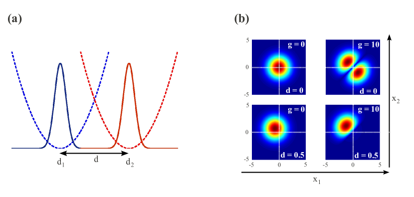
Figure 1: Panel (a) shows a schematic representation of the system at hand [see the Hamiltonian model in Eq. 1]. Panel (b) shows the two-particle probability density for two different distances $d$ between the traps and two distinct values of the scaled interaction strength $g$. The axes are scaled in terms of $a$ as defined in the text.

2 Model Hamiltonian

The model we consider consists of two bosonic atoms confined along the $x$ axis (the axial direction) with two separate, but overlapping harmonic potentials, as shown in Fig. 1(a). The atoms are tightly confined along directions perpendicular to $x$ (the transverse directions) by high-frequency harmonic trapping potentials. As a result of the large energy level separation associated with the transverse confinement, at low temperature the transverse motion is restricted to the lowest mode. The system can then be described by the quasi one-dimensional Hamiltonian

$$\hat{H}= -\frac{\hbar^{2}}{2m_{1}}\nabla^{2}_{1}-\frac{\hbar^{2}}{2m_{2}}\nabla^{2}_{2}+\frac{m_{1}}{2}\omega^{2}(x_{1}-d_{1})^{2}+\frac{m_{2}}{2}\omega^{2}(x_{2}-d_{2})^{2}$$ (1)

$$+g_{1D}\delta(x_{1}-x_{2}),$$

where $m_{1}$ and $m_{2}$ are the masses of the two atoms and $x_{1}$ and $x_{2}$ are their respective spatial coordinates. We assume both traps to have the same frequency $\omega$ and be displaced by the distances $d_{1}$ and $d_{2}$ from the origin of the coordinate system. We model the atomic interaction using the standard point-like pseudo-potential and restrict ourselves to s-wave scattering. At low temperatures the scattering strength is then known to be given by $g_{1D}=-2\hbar^{2}/m_{r}a_{1D}$, where $m_{r}{=}m_{1}m_{2}/(m_{1}{+}m_{2})$ is the reduced atomic mass and $a_{1D}$ is the one-dimensional scattering length related to the actual three-dimensional one via $a_{1D}{=}-a_{\perp}^{2}/2a_{3D}(1-Ca_{3D}/a_{\perp})$. Here $a_{\perp}$ is the size of the single-atom ground state wavefunction in the transversal direction and $C\simeq 1.4603\ldots$ is a constant [10]. By introducing the centre of mass coordinate $X=(x_{1}+x_{2})/2$ and the relative coordinate $x=(x_{1}-x_{2})/2$, the two-atom wavefunction can be factorised into $\phi(X)\psi(x)$ with $\phi(X)$ [$\psi(x)$] being the wavefunction for the centre-of-mass [relative motion] dynamics. Correspondingly, the Schrödinger equation decouples as

$$\left(-\frac{\hbar^{2}}{2M}\frac{\partial^{2}}{\partial X^{2}}+\frac{1}{2}M\omega^{2}X^{2}\right)\phi(X)=\hbar\omega\left(n+\frac{1}{2}\right)\phi(X)\;,$$ (2)

$$\left(-\frac{\hbar^{2}}{2m_{r}}\frac{\partial^{2}}{\partial x^{2}}+\frac{1}{2}m_{r}\omega^{2}(x-d)^{2}+g_{1D}\delta(x)\right)\psi(x)=\hbar\omega\left(\nu+\frac{1}{2}\right)\psi(x)\;,$$ (3)

where we have taken $m_{1}{=}m_{2}{=}m$ for simplicity,and defined $d=d_{1}-d_{2}$, $M=2m$ and $m_{r}=m/2$. Clearly, the centre-of-mass dynamics has the form of simple harmonic motion while the relative problem consists of a displaced harmonic oscillator subjected to a point-like disturbance at the origin of the coordinate system.

For the sake of completeness, in the following we will briefly sketch the steps required to solve Eq. (3). Our approach follows the detailed treatment given in Refs. [13, 14]. For simplicity of notation we first scale all the lengths in units of $a=\sqrt{\hbar/m\omega}$, which is the width of the ground state wavefunction for a single unperturbed particle of mass $m$ along the axial direction of the harmonic trap, and all energies in units of $\hbar\omega$. Eq. (3) thus becomes (for $x\neq 0$)

$$\frac{d^{2}\psi}{d\xi^{2}}+\left(\nu+\frac{1}{2}-\frac{\xi^{2}}{4}-g\,\delta(\xi+d)\right)\psi=0\;,$$ (4)

where $g=g_{1D}a/(\hbar\omega)$ is the renormalised strength of the $\delta$-barrier, $\xi=(x-d)$ is a shifted spatial coordinate and we have dropped the spatial dependence of $\psi$ for convenience. The solutions to this equation can be given in terms of parabolic cylinder functions, $D_{\nu}(\pm\xi)$, of order $\nu$ as follows

$$\psi_{l} =N_{l}D_{\nu}(-\xi) \quad\mbox{for }\;x<0,$$ (5)

$$\psi_{r} =N_{r}D_{\nu}(\xi) \quad\mbox{for }\;x>0,$$ (6)

where $N_{l}$ and $N_{r}$ are the normalization factors that can be calculated by imposing continuity of the solutions at the position of the $\delta$-function. Explicitly, this leads to the following conditions

$$\frac{1}{2}\nu\left[D_{\nu-1}(-d)D_{\nu}(d)+D_{\nu-1}(d)D_{\nu}(-d)\right]-gD_{\nu}(-d)D_{\nu}(d)=0\;,$$ (7)

for non-zero value at the position of the $\delta$-function and

$$N_{r}\nu D_{\nu-1}(-d)+N_{l}\nu D_{\nu-1}(d)=0\;,$$ (8)

whenever the functions are zero at the $\delta$-function. This also determines the energy spectrum of the system, which exhibits trap-induced shape resonances due to energy-level repulsion, as shown in Fig. 2 [13, 14]. Notably, a resonance in the ground state only appears for $g<0$, which is due to the existence of a bound state in this situation (indicated by circle in Fig. 2(a)). The ground-state wavefunction can now be obtained as $\Psi_{0}(x_{1},x_{2})=\phi(X)\psi(x)$ and on the right-hand side of Fig. 1 we show its two particle probability density, $|\Psi_{0}(x_{1},x_{2})|^{2}$. The repulsive interaction between the particles is evident as a zero line along the diagonal in the probability density when $x_{1}=x_{2}$. For a finite trap separation the particles become localised in their respective traps and the two particle probability density moves to occupy the upper left-hand side quadrant.

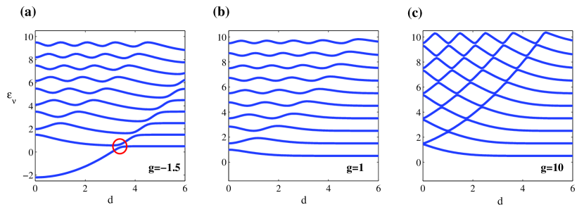
Figure 2: Energy versus distance $d$ between the traps for different values of the scaled interaction strength (a) $g=-1.5$, (b) $g=1$ and (c) $g=10$. For large values of $g$ the energy levels become degenerate at $d=0$. For finite distances between the traps resonances appear whenever two levels approach each other. For a repulsive interaction, the ground state is not affected by such resonances, however, for an attractive interaction, a resonance can be observed (red circle in panel (a)).

From this ground state we are able to explore the zero-temperature quantum correlations of the system by using the von Neumann entropy $S$ of the reduced single-particle density matrix $\rho_{1}(x,x^{\prime})$, which is determined as the kernel of the reduced density operator in configuration space

$$\rho_{1}(x,x^{\prime})=\int_{-\infty}^{\infty}\Psi_{0}(x,x_{2})\Psi^{*}_{0}(x^{\prime},x_{2})dx_{2}\;.$$ (9)

In order to evaluate $S$ we need the eigenvalues $\lambda_{i}$ of $\rho_{1}(x,x^{\prime})$, which are found by numerically solving the integral-value equation

$$\int_{-\infty}^{+\infty}\rho_{1}(x,x^{\prime})\psi_{i}(x^{\prime})dx^{\prime}=\lambda_{i}\psi_{i}(x)\;,$$ (10)

where the $\psi_{i}(x)$ are the eigenstates associated with the $\lambda_{i}$. The von Neumann entropy is then calculated as $S=-\sum_{i}\lambda_{i}\log_{2}\lambda_{i}$ [16, 18, 19]. In Fig. 3 we show $S$ as a function of both the trap distance $d$ and the interaction strength $g$. For the case of a repulsive interaction, it can be seen from Fig. 3(a) that the von Neumann entropy decreases with increasing trap separation. This should be expected as the short range interaction becomes less important and the state of the system tends towards the product state of two non-interacting particles. Fig. 3(b) shows the behaviour of $S$ as a function of the interaction strength, revealing that, after an initial raise, $S$ saturates to an asymptotic value that decreases as $d$ grows. This is again due to the short-range nature of the interaction potential: as the interaction is ineffective for large $d$, the steady value of $S$ would be smaller for increasing values of the separation. For attractive interactions the situation is slightly different and local maxima and saddle points in $S$ can be observed at certain values of the trap separation [see Figs. 3(c) and (d)]. A comparison between Figs. 2 and 3(c) shows the correspondence of the appearance of these stationary points and the existence of the above-mentioned trap induced shape resonances for bound states in the energy spectrum. Such simultaneous occurrences have been observed in all our simulations, and based on their strong numerical evidence we conjecture a relation between stationarity in the von Neumann entropy under attractive potentials and trap-induced shape resonances. While such a connection is rather interesting, it goes beyond the scopes of our work and we reserve to investigate it more deeply in the future. Note that, for a given value of $d$, comparatively smaller values of $g$ are required in the $g<0$ case than in the repulsive one in order to achieve large values of $S$.

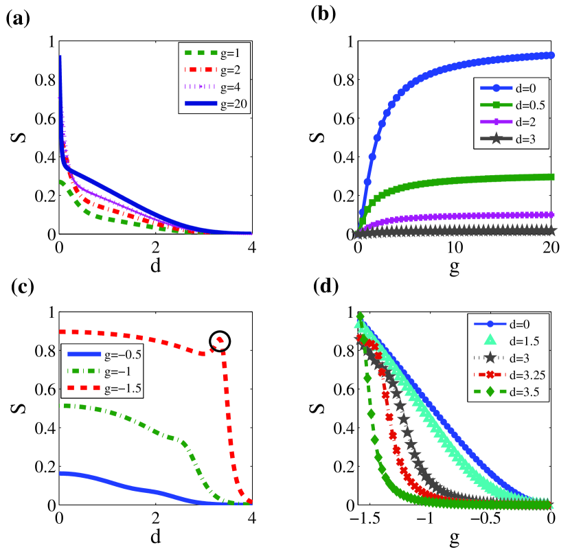
Figure 3: Von Neumann entropy of the ground state for repulsive [panels (a) and (b)] and attractive interaction [panels (c) and (d)]. Plots are shown for the von Neumann entropy versus trap separation, (a) and (c), and von Neumann entropy versus particle interaction strength, (b) and (d). The local maxima visible in (c) and (d) for certain values of $d$ are connected to the appearance of shape induced resonances in the energy spectrum, as seen in Fig. 2(a) for $d\approx 3.5$.

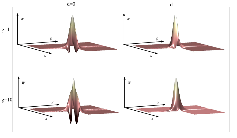
Figure 4: Wigner function for an interaction strength of $g=1$ and $g=10$ at trap separations $d=0$ and $d=1$. A quadrant is removed from the plot to show the negative parts of the Wigner distribution which is symmetric about $p=0$. For $g=1$ a reduction in the negative part of the Wigner function is evident for $d=1$ compared to $d=0$. For $g=10$ the large negative contribution and sharp peak are indicative of the larger interaction strength at $d=0$. For $d=1$ the negative volume is significantly less.

3 Calculation of the Wigner function and assessment of its negativity

We will now investigate the non-classicality of the two-atom state in a much broader range of operative conditions, including finite temperature. For this, the main tool in our study will be the Wigner function associated with the two-particle state. For the specific case at hand, the Wigner function depends on the position and momentum variables $x_{j}$ and $p_{j}$ ($j=1,2$) and is defined as [22]

$$W(x_{1},p_{1};x_{2},p_{2}){=}\!\int d\xi d\varsigma\frac{e^{-\frac{i}{\hbar}p_{1}\xi-\frac{i}{\hbar}p_{2}\varsigma}}{4\pi^{2}\hbar^{2}}\rho\left(x_{1}{+}\frac{\xi}{2},x_{2}{+}\frac{\varsigma}{2},x_{1}{-}\frac{\xi}{2},x_{2}{-}\frac{\varsigma}{2}\right).$$ (11)

By integrating out the momenta or positions one can calculate the marginal spatial or momentum distributions of the two particles, respectively. It is straightforward to include the effects of a non-zero temperature by weighting the higher-order states of the two-atom spectrum with the appropriate Boltzmann factors, $P_{n,\sigma}=\frac{1}{{\cal Z}}e^{\frac{-E_{n,\sigma}}{k_{B}T}}$, where the $E_{n,\sigma}$ are the energies of the atomic eigenstates identified by the centre-of-mass and relative-motion quantum numbers $n$ and $\sigma$, respectively. Moreover, we have introduced the equilibrium temperature of the system $T$, the Boltzmann constant $k_{B}$ and the partition function ${\cal Z}$. We thus get

$$W(\alpha;\beta)=\displaystyle\sum_{n}^{\infty}\displaystyle\sum_{\sigma}^{\infty}P_{n,\sigma}W_{n,\sigma}(\alpha;\beta),$$ (12)

where, for easiness of notation, we have written the Wigner function in terms of the two quadrature variables $\alpha=(x_{1}+ip_{1})/\sqrt{2}$ and $\beta=(x_{2}+ip_{2})/\sqrt{2}$. It is widely accepted that the appearance of negative values in the Wigner function of a system is a strong indication of non-classicality of the associated state. In fact, in this case $W(\alpha;\beta)$ cannot be interpreted as a classical probability distribution describing a microstate in the phase space. Starting from such premises, Kenfack and Zyczkowski have proposed to use the volume occupied by the negative regions of $W(\alpha;\beta)$ as a quantitative indicator for non-classicality (in the sense described above)[23]. Such a (dimensionless) figure of merit can be evaluated as

$$N_{V}=\frac{1}{2}\left(\int_{\Omega}|W(\alpha;\beta)|d\Omega-1\right)$$ (13)

with $\Omega$ being the whole phase-space and $d\Omega=dx_{1}dx_{2}dp_{1}dp_{2}$. Note that in our case the centre-of-mass part of the wavefunction does not depend on the interaction between the particles. Therefore, it does not contribute to the degree of non-classicality and in Fig. 4 we show the Wigner functions associated with only the relative part of our problem for two different values of $g$ and $d$. Negative parts are clearly visible for small values of $d$ and become more prominent for increasing interaction strength. This is also visible in Fig. 5(a), where $N_{V}$ is plotted against $d$. However, the degree of non-classicality decreases faster for a larger interaction strength when the traps are moved apart. The temperature dependence of the negative volume is displayed in Fig. 5(b), where one can see a very fast decrease once the system is able to access states beyond the ground state.

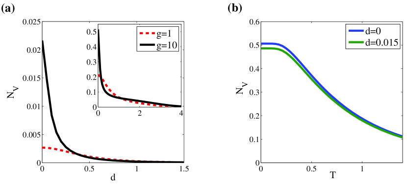
Figure 5: Panel (a) shows the negative volume of the complete Wigner distribution at zero temperature as a function of $d$. The inset shows $N_{V}$ when only considering the contribution to the Wigner function associated with the relative part of the problem. Panel (b) shows the negative volume against increasing temperature (measured in units of $\hbar\omega/k_{B}$) for the relative part of the Wigner distribution with an interaction strength of g=10.

4 Testing non-locality in phase space

The results of the previous Section indicate that a considerable degree of non-classicality might be set in the state of the external degrees of freedom of the two trapped atoms, resilient to some extents to the effects of finite temperature. Moreover, as it should also be clear from Eq. (1), our study has shown the evident non-Gaussian nature of the atomic state (as witnessed by the features of the Wigner function). While correlations in Gaussian states are well and easily characterized, we face the lack of necessary and sufficient criteria for the quantification of entanglement in non-Gaussian states. In fact, the available entanglement measures for CV states are based (to the best of our knowledge) on the use of the negativity of partial transposition criterion formulated in terms of covariance matrices, which carry exact information on the state of a system only in the Gaussian scenario [24]. Interesting criteria based on the use of high-order correlation functions of multi-mode bosonic systems have been proposed, recently [25]. However, the experimental determination of such high-order moments can be cumbersome, requiring multi-port interferometric settings [25]. Since here we would like to provide an operatively feasible test for entanglement in the state of the system at hand we will in the following assess non-classicality in terms of non-locality probed in the phase-space of the system studied here.

We thus consider the CV version of CHSH inequality developed in Ref. [21] and will briefly remind the reader of the key points for completeness. It is well known that the Wigner function calculated at the origin of phase space is equivalent to the expectation value $W(\alpha=0;\beta=0)=\frac{4}{\pi^{2}}\langle\hat{\Pi}_{1}\otimes\hat{\Pi}_{2}\rangle$, where $\hat{\Pi}_{j}$ is the parity operator for mode $j=1,2$  [26]. The total Wigner function can therefore be written by using displaced parity operators as [26]

$$W(\alpha;\beta)=\frac{4}{\pi^{2}}\langle\hat{D}_{1}(\alpha)\hat{\Pi}_{1}\hat{D}_{1}^{\dagger}(\alpha)\otimes\hat{D}_{2}(\beta)\hat{\Pi}_{2}\hat{D}_{2}^{\dagger}(\beta)\rangle,$$ (14)

where $\hat{D}_{j}(\alpha)$ is a displacement operator for mode $j$ of amplitude $\alpha$ [24]. A CHSH-like function can then be built starting from the above as

$$\mathcal{B}=\frac{\pi^{2}}{4}[W(0;0)+W(\sqrt{\mathcal{J}};0)+W(0;-\sqrt{\mathcal{J}})-W(\sqrt{\mathcal{J}};-\sqrt{\mathcal{J}})]$$ (15)

with ${\cal J}$ a positive constant. Local realistic theories impose $|{\cal B}|\leq{2}$ [21] and any value outside this range indicates non-local behaviour.

Equipped with these tools, we can now quantitatively study the non-locality in the state of our system. Using the Wigner function calculated in Sec. 3, we determine the violation of the CHSH inequality optimised over $\mathcal{J}$ and study the behaviour of ${\cal B}$ against the interaction strength between the particles and the distance between the traps. In Fig. 6(a) we show the numerically optimised values of $\mathcal{B}$ against $d$ for various interaction strengths $g$ and at zero temperature. Clearly, for short distances the violation of the local realistic bound is larger for strong interactions. The situation is somehow reverted at large distances, where weakly interacting atomic pairs appear to violate the CHSH inequality more significantly. Such an apparently counterintuitive result can be understood by reminding one that the one-dimensional interaction strength is inversely proportional to the one-dimensional scattering length (see Sec. 2): a lower value of $g$ corresponds to a larger scattering length. This means that while the correlations steaming from the reduced dimension decay with increasing distance, the influence of the scattering length persists for larger values of $d$. Comparing these results to the von Neumann entropy shown in Fig. 3 it is evident that achieving a non-zero von Neumann entropy does not necessarily correspond to the violation of CHSH inequality, in qualitative agreement with the findings of Ref. [16]. It would be interesting to compare the behaviour found here with those corresponding to longer-range interaction potentials which might well lead to sustained non-locality at larger distances. In Fig. 6(b) we show ${\cal B}$ as a function of the interaction strength. The non monotonic behaviour of the CHSH function against the interaction strength, as well as the disappearance of any violation at finite values of $g$ and for $d\neq{0}$, are striking. It can be understood by realising that the offset between the traps breaks the symmetry of the system and a large repulsive interaction between the particles results in less overlap and therefore less correlations in the phase space. Noticeably, although the CHSH inequality is only violated for $d\lesssim 0.08$, recent experiments involving optical lattices have demonstrated the possibility to off-set atomic trapping potentials with an accuracy of exactly this order of magnitude [27].

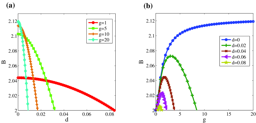
Figure 6: The violation of the CHSH inequality at $T=0$ is shown in panel (a) against trap separation for various interaction strengths and in (b) versus $g$, for increasing trap separations.

For the case of non-zero temperature we plot the violation of the CHSH inequality for two values of interaction strengths ($g=1,10$) in Fig. 8. While the similarity of the plots shows the general trends of decay of the correlations with increasing temperature and distance, one can note that for $g=1$ the system is more resilient to the effects of an increasing temperature than in the stronger-interaction case because the separations between neighbouring energy levels increases at low $\delta$-barrier (i.e. small $g$’s). At large $g$, this implies a greater probability to excite higher-energy modes at small temperature. Evidently, the violation of CHSH inequality becomes very sensitive to temperature variations once the thermal energy is comparable to the energy-level separation.

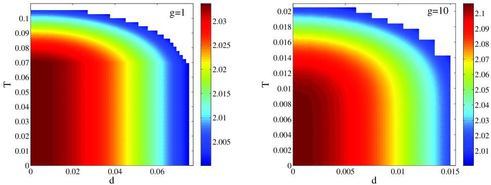
Figure 7: Degree of CHSH violation against trap-separation and temperature (in units of $\hbar\omega/k_{B}$) for interaction strengths of $g=1$ and $g=10$. The change in temperature has a greater impact on the two particles at greater interaction energies (note the different scalings in the two plots).

We conclude this Section by sketching a strategy for the reconstruction of the atomic Wigner function for a non-locality test following the approach suggested by Lutterbach and Davidovich [28]. The key is mapping the information encoded in the external degree of freedom of one of the trapped atoms into specific internal state of the atom itself, which can then be efficiently read out. For the sake of argument, let us for the moment address the case of a single atom and label the logical states of the qubit as $\{|{\uparrow}\rangle,|{\downarrow}\rangle\}$. Physically, they could be two quasi-degenerate metastable ground states of a three-level $\Lambda$-like model and transitions from each ground state to the excited level of the $\Lambda$ model will induce motional state-dependent sidebands are induced on $|{\uparrow}\rangle$ and $|{\downarrow}\rangle$. The transition between different motional states of the atom can thus be induced by properly tuned stimulated Raman passages connecting two different sidebands of the ground-state doublet, as described in [29], in a way so as to mimic the dynamics intertwining motional degrees of freedom and internal ones in trapped ions. Such processes can be performed with an almost ideal efficiency. Working in an appropriate Lamb-Dicke limit (where the recoil energy due to the kicks induced by the coupling between atomic levels and light is much smaller than the ground-state energy of the motional mode), it is possible to relate the difference $P_{\uparrow}-P_{\downarrow}$ between the probability of finding the atom in $|{\uparrow}\rangle$ or $|{\downarrow}\rangle$, respectively, to the expectation value of the displaced parity operator and thus, in turn, to the value of the Wigner function at a given point of the phase space [28]. Such a difference in probability can be effectively measured by means of routinely implemented high-efficiency fluorescence light-based detection methods [30]. In order to reconstruct the two-atom Wigner function, it would be sufficient to collect signals from both the atoms undergoing similar reconstruction protocols and appropriately putting together the statistical data gathered. In doing this, distinguishability of the signals collected from the two particles can be attained by using fluorescence cycles of different frequencies, one per particle. In this way, one can distinguish the statistics associated with a specific particle without the need of separating the corresponding traps by a large distance.

5 Effects of dissipation

Let us finally discuss the influence of a general loss mechanisms, one per atomic mode, that may affect the two-atom state due to finite-time coherence of the external degrees of freedom. Such a lossy process can be effectively modelled considering each atomic vibrational mode as in contact with a background bath of bosons (due, for instance, to mode-mode coupling induced by an-harmonicity of the traps or position-to-electric-field coupling induced by stray electromagnetic fields in the proximity of the trapped particles) [31]. The master equation arising from such a coupling can be then tackled by transforming it into a Fokker-Planck equation, which has exactly the same form as the one describing the propagation of an optical mode in a lossy channel [32]. Alternatively, our study could equivalently be used so as to take into account the effects of a finite-efficiency detection apparatus for the non-locality test (although fluorescence-based methods have very high efficiency, boosted up with respect to single-photon detection efficiency by the large number of photons carried by the fluorescence signal, ideality of signal-collection is not yet achieved). Both models can be abstractly yet rigorously described by considering a simple beam-splitter model as follows: assuming low temperature environments allows us to describe them as two independent zero-$T$ bosonic baths, each prepared in its collective vacuum state. We call $A$ ($B$) the environmental bath affecting mode $1$ ($2$). The Wigner function of the vacuum state of each is

$$W_{0}(\mu_{k})=\frac{2}{\pi}e^{-2|\mu_{k}|^{2}}~{}~{}~{}(k=A,B),$$ (16)

where $\mu_{k}=\frac{{x}_{k}+i{p}_{k}}{\sqrt{2}}$ are the quadrature variables of the environmental modes. The interaction between the signal mode $j$ and its environment is modelled as a mixing at a beam splitter having reflectivity $\eta_{k}$. For simplicity and without affecting the generality of our discussions, we assume the reflectivity to be equal in both modes, $\eta_{k}=\eta$. In phase space, the state of the signal mode after the interaction and after tracing over the environmental degrees of freedom is described by the convolution

$$W^{\eta}(x_{1},x_{2},p_{1},p_{2}) {=}\!\int dx_{A}dx_{B}dp_{A}dp_{B}W(\tilde{x}_{1},\tilde{p}_{1},\tilde{x}_{2},\tilde{p}_{2})$$ (17)

$$\quad\times W_{0}(\tilde{x}_{A},\tilde{p}_{A})W_{0}(\tilde{x}_{B},\tilde{p}_{B}),$$

where we have introduced the transformed variables

$$\tilde{x}_{j} =\sqrt{\eta}\,x_{j}-\sqrt{1-\eta}\,x_{k},~{}~{}\tilde{x}_{k}=\sqrt{\eta}\,x_{k}+\sqrt{1-\eta}\,x_{j},$$ (18)

$$\tilde{p}_{j} =\sqrt{\eta}\,p_{j}-\sqrt{1-\eta}\,p_{k},~{}~{}\tilde{p}_{k}=\sqrt{\eta}\,p_{k}+\sqrt{1-\eta}\,p_{j}$$ (19)

and one should take $k=A$ ($B$) if $j=1$ ($2$). Eq. (17) is evaluated numerically and used to test violation of the CHSH inequality against $\eta$. Needless to say, the effect of losses (or detection inefficiencies) is to reduce the degree of violation of the CHSH inequality, as shown by the solid blue lines in Fig. 8. The same trend highlighted before regarding resilience of non-locality properties for lower values of $g$ is retrieved here.

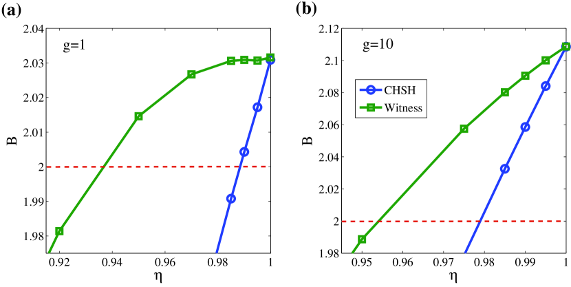
Figure 8: Plots of CHSH violation and entanglement witness for interaction strengths of $g=1$ (panel (a)) and $g=10$ (panel (b)) with inefficiency $\eta$. The violation of CHSH is seen to decay quickly as the detection becomes inefficient (blue lines), however the entanglement witness (green lines) shows the existence of entanglement for greater inefficiencies, with the lower value of $g$ having more resilience to the losses.

It is therefore highly desirable to design viable strategies for a more robust analysis of non-locality. A step in this direction has been recently performed in Ref. [33] with the proposal of a robust entanglement witness based on a CHSH-like inequality that shows resilience with respect to losses/detection inefficiencies of the form considered here. Following the derivation provided by Lee et al. [33], one can see that for separable bipartite states and loss rate/detection inefficiency $\eta$, the following inequalities hold

$$\mid\langle\mathcal{{W}}_{\eta>\frac{1}{2}}\rangle\mid {=}|\frac{\pi^{2}}{4\eta^{2}}[W^{\eta}(0,0){+}W^{\eta}(0,-\sqrt{\mathcal{J}}){+}W^{\eta}(\sqrt{\mathcal{J}},0){-}W^{\eta}(\sqrt{\mathcal{J}},-\sqrt{\mathcal{J}})]$$

$$+\frac{\pi(\eta-1)}{\eta^{2}}[W^{\eta}_{\alpha}(0)+W^{\eta}_{\beta}(0)]+2(1-\frac{1}{\eta})^{2}|\leq 2,$$

$$\mid\langle\mathcal{{W}}_{\eta\leq\frac{1}{2}}\rangle\mid {=}|\pi^{2}[W^{\eta}(0,0)+W^{\eta}(0,-\sqrt{\mathcal{J}})+W^{\eta}(\sqrt{\mathcal{J}},0)-W^{\eta}(\sqrt{\mathcal{J}},-\sqrt{\mathcal{J}})]$$ (20)

$$-2\pi[W^{\eta}_{1}(0)+W^{\eta}_{2}(0)]+2|\leq 2.$$

Here, $W^{\eta}(a,b)$ is the two-mode Wigner function calculated in Eq. (17) and $W^{\eta}_{1,2}$ are its single-mode marginals. For the case of perfect detectors ($\eta=1$) the inequality becomes equivalent to (15). It is apparent that any violation of this inequality for $\eta<1$ ensures the violation of the CHSH-inequality in the presence of the unitary case as well, thus such witness can be used effectively for detecting entanglement in the presence of noise. From the results shown in Fig. 8 one can see that, while the CHSH inequality violation is lost for $\eta=0.98$ at $g=10$, the entanglement witness still violates it at $\eta\simeq 0.95$, which is a small yet significant improvement. It is important to notice that current avalanche photodiodes used to collect fluorescence have quantum efficiencies exactly in this range. Interestingly the entanglement witness for $g=1$ is violated for smaller $\eta$, echoing the trend noticed for the CHSH at zero and non-zero temperature: lower interaction strengths give rise to states more resilient to influences from the environment.

6 Conclusions

We have investigated CV entanglement in a system of two interacting bosons in separate harmonic trapping potentials under a variety of conditions. We have found that the von Neumann entropy shows strong correlations at zero temperature and shown violation of local realistic theories for a wide range of relevant parameters. An interesting and rather counterintuitive behavior has been observed, even at non-zero temperature, for the whole range of interaction strengths analysed. We have related the multiple facets of both the revealed non-locality and the von Neumann entropy to the details of the coupling model used in this work and the corresponding spectrum of the system.

Finally, we have included the effects of general non-idealities (such as dissipative losses affecting the motional degrees of freedom of the trapped atoms or inefficient detectors), demonstrating the fragility of the atomic non-locality. In order to circumvent such a hindrance, we have shown that some improvements can come from the use of a recently proposed entanglement witness that fits very well with the general approach put forward here. We hope that the realistic nature of our proposal functions as a significant model to test non-classicality of massive systems. Since it is rather close to state of the art experimental possibilities we expect it to spur experimental interest in the study of non-classical behaviour of simple low-dimensional atomic systems under non-ideal working conditions.

7 Acknowledgements

We acknowledge financial support from the Irish Research Council for Science and Engineering under the Embark initiative RS/2009/1082 and Science Foundation Ireland under grants no. 05/IN/I852 and 05/IN/I852 NS. JG would like to thank the National Research Foundation and Ministry of Education of Singapore for support and Mr. G. Vacanti for interesting discussions. MP is grateful to Dr. Seungwoo Lee and Prof. Hyunseok Jeong for invaluable comments and thanks the UK EPSRC for financial support (EP/G004579/1).

8 Bibliography

References

- [1] I. Bloch, J. Dalibard and W. Zwerger, Rev. Mod. Phys. 80, 885 (2008).
- [2] C. Chin, R. Grimm, P. Julienne, Rev. Mod. Phys. 82, 1225 (2010).
- [3] J. Beugnon, M. P. A. Jones, J. Dingjan, B. Darquié, G. Messin, A. Browaeys and P. Grangier, Nature 440, 779 (2006).
- [4] M. Anderlini, P. J. Lee, B. L. Brown, J. Sebby-Strabley, W. D. Phillips and J. V. Porto, Nature 448, 452 (2007).
- [5] T. Wilk, A. Gaëtan, C. Evellin, J. Wolters, Y. Miroshnychenko, P. Grangier and A. Browaeys, Phys. Rev. Lett. 104, 010502 (2010).
- [6] D. Jaksch, H.-J. Briegel, J. I. Cirac, C. W. Gardiner, and P. Zoller, Phys. Rev. Lett. 82, 1975 (1999).
- [7] T. Calarco, E. A. Hinds, D. Jaksch, J. Schmiedmayer, J. I. Cirac, and P. Zoller, Phys. Rev. A 61, 022304 (2000).
- [8] L. Isenhower, E. Urban, X. L. Zhang, A. T. Gill, T. Henage, T. A. Johnson, T. G. Walker, and M. Saffman, Phys. Rev. Lett. 104, 010503 (2010).
- [9] O. Mandel, M. Greiner, A. Widera, T. Rom, T.W. Hänsch and I. Bloch, Phys. Rev. Lett. 91, 010407 (2003)
- [10] M. Olshanii, Phys. Rev. Lett. 81, 938 (1998).
- [11] K. Huang and C. N. Yang, Phys. Rev. 105, 767 (1957).
- [12] Th. Busch, B. G. Englert, K. Rzazewski, and M. Wilkens, Found. Phys. 28, 549 (1998).
- [13] M. Krych and Z. Idziaszek, Phys. Rev. A 80, 022710 (2009).
- [14] J. Goold, M. Krych, T. Fogarty, Z. Idziaszek and Th. Busch, New J. Phys. 12 093041 (2010).
- [15] T. Stöferle, H. Moritz, K. Günter, M. Köhl and T. Esslinger, Phys. Rev. Lett. 96, 030401 (2006).
- [16] H. Mack and M. Freyberger, Phys. Rev. A 66, 042113 (2002).
- [17] M. Bußhardt and M. Freyberger, Phys. Rev. A 75, 052101 (2007).
- [18] B. Sun, D. Zhou and L. You, Phys. Rev. A. 73, 012336 (2006).
- [19] D. S. Murphy, J. F. McCann, J. Goold, and Th. Busch, Phys. Rev. A. 76, 053616 (2007).
- [20] J. Goold, L. Heaney, Th. Busch, and V. Vedral Phys. Rev. A. 80, 022338 (2009).
- [21] K. Banaszek and K. Wodkiewicz, Phys. Rev. A 58, 4345 (1998); Phys. Rev. Lett. 82 2009 (1999).
- [22] E. P. Wigner, Phys. Rev 40, 749 (1932).
- [23] A. Kenfack and K. Życzkowski, J. Opt. B: Quantum Semiclass. Opt. 6, 396 (2004).
- [24] S. L. Braunstein and P. van Loock, Rev. Mod. Phys. 77, 513 (2005).
- [25] E. V. Shchukin and W. Vogel, Phys. Rev. A 72, 043808 (2005); Phys. Rev. Lett. 95, 230502 (2005).
- [26] A. Royer, Phys. Rev. A 15, 449 (1977).
- [27] L. Förster, M. Karski, J.-M. Choi, A. Steffen, W. Alt, D. Meschede, A. Widera, E. Montano, J.H. Lee, W. Rakreungdet, and P. S. Jessen, Phys. Rev. Lett. 103, 233001 (2009).
- [28] L. G. Lutterbach and L. Davidovich, Phys. Rev. Lett. 78, 2547 (1997).
- [29] A. S. Parkins and E. Larsabal, Phys. Rev. A 63, 012304 (2000); M. Paternostro, M. S. Kim, and P. L. Knight, Phys. Rev. A 71, 022311 (2005).
- [30] C. Monroe, D. M. Meekhof, B. E. King, and D. J. Wineland, Science 272, 1131 (1996).
- [31] D. Leibfried, R. Blatt, C. Monroe, and D. Wineland, Rev. Mod. Phys. 75, 281 (2003).
- [32] D. F. Walls, and G. J. Milburn, “Quantum Optics” (Springer, Berlin, 2008).
- [33] S. W. Lee, H. Jeong and D. Jaksch, Phys. Rev. A. 81, 012302 (2010).