Recurring millimeter flares as evidence for star-star magnetic reconnection events in the DQ Tau PMS binary system

Observations of the T Tauri spectroscopic binary DQ Tau in April 2008 captured an unusual flare at 3 mm, which peaked at an observed maximum flux of $\sim$0.5 Jy (about 27 times the quiescent value). Here we present follow-up millimeter observations that demonstrate a periodicity to the phenomenon. While monitoring 3 new periastron encounters, we have detected flares within 17.5 hours (or 4.6%) of the orbital phase of the first reported flare and constrained the main emitting region to a stellar height of 3.7–6.8 R_⋆. The recorded activity is consistent with the proposed picture for synchrotron emission initiated by a magnetic reconnection event when the two stellar magnetospheres of the highly eccentric ($e$ = 0.556) binary are believed to collide near periastron as the stars approach a minimum separation of 8 R_⋆ ($\sim$13 R_⊙). The similar light curve decay profiles allow us to estimate an average flare duration of 30 hours. Assuming one millimeter flare per orbit, DQ Tau could spend approximately 8% of its 15.8-day orbital period in an elevated flux state. These findings continue to serve as a small caution for millimeter flux points in spectral energy distributions that could contain unrecognized flare contributions. Our analysis of the millimeter emission provides an upper limit of 5% on the linear polarization. We discuss the extent to which a severely entangled magnetic field structure and Faraday rotation effects are likely to reduce the observed polarization fraction. We also predict that, for the current picture, the stellar magnetospheres must be misaligned at a significant angle or, alternatively, that the topologies of the outer magnetospheres are poorly described by a well-ordered dipole inside a radius of 7 R_⋆. Finally, to investigate whether reorganization of the magnetic field during the interaction affects mass accretion, we also present simultaneous optical (VRI) monitoring of the binary, as an established tracer of accretion activity in this system. We find that an accretion event can occur coincident in both time and duration with the synchrotron fallout of a magnetic reconnection event. While the pulsed accretion mechanism has been attributed previously to the dynamical motions of the stars alone, the similarities between the millimeter and optical light curves evoke the possibility of a causal or co-dependent relationship between the magnetospheric and dynamical processes.

1 Introduction

Pre-main-sequence (PMS) stars are characterized by variability in most wavebands. At millimeter wavelengths, however, the dominant emission process is the optically thin, thermal radiation from the dust located in a circumstellar disk. The integrated flux is therefore a measure of the total amount of cold circumstellar material, which evolves on timescales of roughly 10⁶ years. Before the discovery of the first strong millimeter flare toward the young stellar object (YSO) GMR-A in Orion (Bower et al. 2003; Furuya et al. 2003), pronounced short-term millimeter variability was undocumented even though radio variability is well known toward YSOs (e.g. Stine et al. 1988; White et al. 1992). The lack of millimeter variability studies in the literature is in large part due to the time-consuming nature of observations at these wavelengths, leading to few follow-up measurements. As a result, DQ Tau is only the fourth YSO to be recognized in outburst at millimeter wavelengths. The initial serendipitous detection occurred during an 8-hour observation on 2008 April 19, when the source brightened at 3 mm (115 GHz) in a matter of hours to reach a maximum detected flux of 468 mJy, in comparison to a quiescent value of 17 mJy in the adjacent days (Salter et al. 2008). The flare mechanism was attributed to synchrotron emission from a powerful magnetic reconnection event, probably due to the colliding magnetospheres of the binary components near periastron; and similar in nature to the interacting coronae evidenced toward another millimeter-flaring PMS star V773 Tau A (Massi et al. 2002, 2006, 2008).

DQ Tau ($\alpha_{\rm 2000}$ = 04:46:53.06, $\delta_{\rm 2000}$ = $+$17:00:00.1) is a double-lined spectroscopic binary that consists of two relatively equal-mass stars ($\sim$0.65 M_⊙) of similar spectral type (in the range of K7 to M1); as summarized in Table 1. Its highly eccentric ($e$ = 0.556) orbit means that the two stars approach to within 8 R_⋆ ($\sim$13 R_⊙) at periastron (Mathieu et al. 1997). This makes the system unique in terms of magnetic reconnection events because the minimal separation of the binary is on the order of the theoretical T Tauri stellar magnetospheric radius of $\sim$5 R_⋆ (Shu et al. 1994; Hartmann et al. 1994). This radius is generally defined as the range within which the stellar magnetic field lines remain closed, meaning that the field lines both begin and end at the stellar surface. As a result, the geometry of the system alone predicts an overlap of the two magnetospheres at each periastron event; and as the stars approach one another it may become energetically more stable for the fields to briefly merge together. Field lines rooted on one star break and instantly reconnect with the field lines rooted on the companion, releasing magnetic energy into the surrounding region in the process (Vasyliunas 1975; Hesse & Schindler 1988).

Magnetic reconnection events like these are still a poorly understood phenomenon. They occur most notably within the solar corona when oppositely-directed field lines are forced together, typically above magnetically active regions where closed magnetic loops, anchored in sunspots, interact with one another (Haisch et al. 1991). The associated millimeter emission is explained as the superposition of a gyro-synchrotron spectrum with synchrotron emission (Kaufmann et al. 1986), powered by the re-organization of the field lines as they relax into a lower energy state. This solar analogy helps form the basic principles for our stellar scenarios, which can also include magnetic interactions between a star and its accretion disk or a star and a planet forming within its circumstellar disk (Phillips et al. 1991). A consistent flare timing near periastron, however, is a strong indicator that both stellar magnetospheres—as the strongest and most stable magnetic structures in the binary system—are contributors to the transient millimeter activity seen toward DQ Tau.

Here we report on 3 additional flares captured toward this system and discuss what these events mean for the current interpretation of a periodic, star-star magnetic reconnection phenomenon. Our aim is to constrain the nature and regularity of the millimeter emission mechanism by addressing variations in the timing of the flare during the orbit, the duration of the flares, their peak strengths, and the degree of polarization present. For the most recent millimeter flare, X-ray observations were performed in parallel and these will be discussed separately in Getman et al. (2010, submitted). In addition, periastron events in this system are characterized by variable accretion bursts, most likely driven by the dynamical motions of the binary components (Artymowicz & Lubow 1996). Therefore, a secondary goal of this work is to explore the relative timing of the two interactions, dynamical and magnetospheric, acknowledging that the two mechanisms may exist independently and only share the common periodicity of the binary orbit. To probe the accretion mechanism we present and analyze simultaneous optical photometry measurements, which have been shown to be excellent tracers of the accretion activity in this system (see Basri et al. 1997; Mathieu et al. 1997).

2 Observations and data reduction

2.1 Millimeter interferometry

In the follow-up millimeter observations presented here, we chose to observe at slightly lower frequencies in the 3 mm band (90–95 GHz) than those specified during the initial discovery (115 GHz). This strategy takes advantage of greater instrument sensitivities toward lower frequencies and the higher ratio of non-thermal to thermal emission expected toward longer wavelengths. We also supplement the 3 mm band data with a simultaneous observation in the 1 mm band (238 GHz), in order to probe the spectral slope of the transient emission. The technical details for each millimeter data set—all scheduled for observation in the 24-hour period before a periastron event—are summarized in the text below and in Table 2. While each millimeter facility may respond differently to a high degree of polarization as its linear feeds rotate while tracking the source, we show in Sect. 4.2 that the polarization fraction is minimal and therefore does not affect the measurements presented here.

Table 1: DQ Tau Binary System Parameters

System Parameter	Value	Source
Stellar Radius [R⊙]	1.6	1
Stellar Mass [M⊙]	0.65	1
Rotation Period [days]	$\sim$3	2
Orbital Period [days]	15.8043	1
Orbital Eccentricity	0.556	1
Inclination [∘]	157	3
Periastron Separation [R⊙]	13	1
Apoastron Separation [R⊙]	56	1

Sources. 1. Mathieu et al. (1997); 2. Basri et al. (1997); 3. Boden et al. (2009).

Table 2: Millimeter observing log

UT Date	Observatory	Array	Antennas	Baselines	$\nu_{c}$	Bandwidth	H.A. Range	Optical	X-ray
[track start]		Config.		[k$\lambda$]	[GHz]	[GHz]	[hrs]	Data	Data
2008 Dec 28	IRAM	B	1, 2, 4, 5, 6	26–136	90.0	1.0	-2.9 to 5.3	Yes	No
2009 Mar 17	IRAM	C	All	7–53	90.0	1.0	-4.1 to 4.1	No	No
2010 Jan 11	IRAM	A	All (Ant. 4 fails at 22:30h)	48–228	90.0	1.0	-2.6 to 5.9	Yes	Yes
2010 Jan 12	CARMA	B	1, 2, 3, 4, 5, 8, 9, 10, 13, 14	36–292	92.5	3.0	-3.2 to 5.2	No	Yes
2010 Jan 12	SMA	Ext.	All	27–179	238.5	4.0	-3.7 to 4.8	No	Yes

IRAM PdBI. Located in the French Alps, the IRAM Plateau de Bure Interferometer (PdBI) is a 6-element millimeter array capable of measuring two linear polarization directions. We observed DQ Tau at 90 GHz ($\approx$ 3.3 mm) on 3 separate UT dates: 2008 December 28-29, 2009 March 17, and 2010 January 11-12. Each observation (or track) was approximately 8 hours in length and, aside from the array configuration on each UT date, the observations had identical receiver setups of 2$\times$ 1 GHz (V $+$ H dual-polarization) in full-bandwidth mode (4$\times$ 320 MHz overlapping quarters). The same standard calibration method was applied to all three tracks: we used the radio source 3C84 for both the passband and flux calibration, and we observed the gain calibrators 0507+179 (a polarized source) and 0446+112 for 2.25 min (45 sec $\times$ 3 scans) each between every 22.5-min (45 sec $\times$ 30 scans) on-source observation. All data sets were processed using the GILDAS CLIC and MAPPING reduction software, developed by the Grenoble Astrophysics Group. To extract the flux density, we assumed a model for a point source and we averaged the weighted visibilities for all baselines in 90-sec time steps. The error bars displayed per flux point represent the 1$\sigma$ deviation from the average value. Finally, maps for each track were produced using a natural weighting in the inversion step, and Hogbom cleaning was performed down to the RMS level of the dirty maps.

CARMA. We observed DQ Tau in the 3 mm band with the Combined Array for Research in Millimeter-wave Astronomy (CARMA) on UT 2010 January 12. This observation overlapped for 1.5 hours with the end of the third IRAM track, providing continuous coverage on this date for an 18-hour period during a simultaneous Chandra X-ray observing campaign (see Getman et al., submitted). Located in eastern California (USA), CARMA is a heterogeneous interferometer comprised of 23 antennas: six 10.4-m telescopes from the California Institute of Technology/Owens Valley Radio Observatory (OVRO), nine 6.1-m telescopes from the Berkeley-Illinois-Maryland Association (BIMA), and eight 3.5-m telescopes from the University of Chicago Sunyaev-Zel’dovich Array (SZA). Our program was executed while the antennas were being moved out of the CARMA B configuration, and only 10 of the 6-m and 10-m antennas were available to provide baselines between 117 and 946 m. We used the CARMA Paired Antenna Calibration Systems (C-PACS) to compensate for the rapid phase fluctuations on the long baselines. In the C-PACS observing mode, the CARMA 6-m and 10-m antennas observe the phase calibrator and science target as for normal interferometric observations. Simultaneously, the CARMA 3.5-m antennas observe a bright source at a frequency of 30 GHz to monitor the atmospheric fluctuations. The observed phase fluctuations at 30 GHz were then used to calibrate the observed phases toward DQ Tau, and thereby reduce the flux loss due to atmospheric de-correlation on the longer baselines. A detailed description of C-PACS and the data reduction procedures are presented in Pérez et al. (2010, in prep). For our observations, the observing cycle consisted of 3-min observations of the gain calibrator 0530$+$135 by both sets of antennas. Then, while the 6-m and 10-m antennas observed DQ Tau for 15 min, the 3.5-m antennas observed the calibrator 0440$+$146. We used 3C273 for the passband flattening and Uranus for flux calibration. The correlator for the 6-m and 10-m antennas was configured with three 500 MHz bands (or 1.5 GHz) per sideband that covered the frequencies 89.2–90.7 GHz in the lower sideband and 94.2–95.7 GHz in the upper sideband. The data were processed using the MIRIAD data reduction software program, optimized for CARMA. In MIRIAD we used uvfit for a point source to determine the flux value and error for time intervals of 5 min. For mapping we again used a natural weighting for the $u,v$-coverage in the inversion step and cleaning was performed down to 1.5$\sigma$ (where $\sigma$ is the theoretical sensitivity) using the MOSSDI2 package.

SMA. The Submillimeter Array (SMA) is an 8-element array located on the summit of Mauna Kea in Hawaii. We observed DQ Tau at the higher frequency of 238.5 GHz ($\approx$ 1.3 mm), also on 2010 January 12, to achieve an 8-hour overlap with the CARMA track. The array was in its ‘Extended’ configuration, providing 27 baselines spanning 34 to 225 m. The 4 GHz bandwidth was uniformly sampled with 128 channels per chunk and a total of 48 chunks. At the start of the night, the opacity was measured independently and the precipitable water vapor (PWV) was estimated to be around 1 mm, rising to 1.3 mm at the end of the track. Scans were shortened to 15 sec while in the extended configuration, and the source was observed for 7.5-min integration loops. The gain calibrators 0423$-$018, 0530$+$135, and 0510$+$180 were observed for 3 min after every on-source loop. The flux scale was checked every 3 hours with an observation of Uranus or Mars, and the calibrator 3C273 was used to correct for the passband. The data were reduced using the MIR package for IDL, provided by the Smithsonian Astrophysical Observatory, and subsequently analyzed using the uvfit package of the MIRIAD data reduction software program.

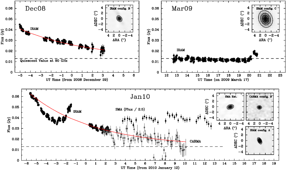
Figure 1: The millimeter fluxes versus time for DQ Tau, as observed with the IRAM PdBI, CARMA, and SMA on 2008 December 28-29 (upper left), 2009 March 17 (upper right), and 2010 January 11-12 (lower panel). All fluxes have been determined from a fit to the visibilities using a point source model. Each IRAM data point represents an on-source time interval of 1.5 min. The CARMA and SMA (divided by 2.5) values are for 5-min intervals. The light curves reveal a (track-averaged) quiescent flux level of 13 mJy at 90 GHz during the March IRAM observation and 97 mJy at 238.5 GHz for the January SMA observation. During the December and January observations, we caught the flare decay phase and fitted an (identical) exponential decay with an e-folding time of 6.55 hours (solid red line) to both light curves. We note that the fit does not apply to the initial decay of the original April 2008 light curve (see Sect. 3.1). The March observation only indicates elevated activity near the end of the track, which we take to be the start of a flare. In the upper right-hand corner of each panel, we give the (unresolved) continuum images for the entire track where the continuum contours are drawn for 3$\sigma$ levels and each $\sigma$ is of the order 1 mJy bm^-1.

Table 3: Millimeter track and light curve statistics

UT Date	Track ID	Beam Size	$\nu_{c}$	Fstart	Fend	$\sigma_{avg}$	Linear	Orbital Phase	Hours from	$t$ = 0
		[′′]	[GHz]	[mJy]	[mJy]	[mJy]	Polariz.	Coverage [$\Phi$]	Periastron (0.0)	[$\Phi$]
2008 Dec 28	Dec08-IRAM	1.34 $\times$ 1.02	90.0	43.0	20.2	1.2	$<$ 4.65%	-0.02 to 0.00	$-$6.8 to 1.5	-0.056
2009 Mar 17	Mar09-IRAM	3.39 $\times$ 2.79	90.0	12.6	16.9	1.1	$<$ 8.15%	-0.03 to -0.01	$-$13.7 to $-$5.3	-0.007
2010 Jan 11	Jan10-IRAM	1.32 $\times$ 0.70	90.0	62.4	29.2	1.1	$<$ 7.60%	-0.04 to -0.02	$-$14.4 to $-$6.5	-0.067
2010 Jan 12	Jan10-CARMA	0.87 $\times$ 0.67	92.5	30.3	12.4	3.9	-	-0.02 to 0.00	$-$7.2 to 1.1	-0.067
2010 Jan 12	Jan10-SMA	1.25 $\times$ 1.00	238.5	95.6	85.2	5.6	-	-0.01 to 0.01	$-$4.7 to 3.6	-0.067
2008 Apr 19	Apr08-CARMA	3.66 $\times$ 1.00	113.1	468	194	-	-	-0.02 to -0.01	$-$8.7 to $-$2.7	-0.020

2.2 Optical photometry

Optical monitoring of DQ Tau during the first IRAM track on 2008 December 28 was performed simultaneously from the Wellesley College 0.6-m telescope in Wellesley, MA (USA) and the IAC80 0.8-m telescope of Teide Observatory, located in the Canary Islands (Spain). Optical coverage in 2 locations allowed us to monitor DQ Tau throughout the 8-hour millimeter track, and for several hours thereafter. We also obtained simultaneous optical (Teide) and millimeter (IRAM) observations for the final follow-up observation on 2010 January 11. To complete the optical characterization of DQ Tau, additional monitoring was carried out from Wellesley and from Teide Observatory in the one-month period from December 2008 to January 2009 (covering the weeks before and after the first millimeter follow-up observation). For part of the observations at Wellesley, DMS was a visiting astronomer, while the observations at Teide Observatory were executed in service mode as part of the IAC80 EXTRA observing program for small projects. A complete listing of the optical measurements is provided in Table 4 online.

The detector used during the Teide observations was CAMELOT, a 2048$\,{\times}\,$2048 back-illuminated CCD chip with a 0.304^′′ pixel scale, corresponding to a 10.4${}^{\prime}{\times}$10.4^′ field of view. The detector on the Wellesley telescope was a 1024$\,{\times}\,$1024 CCD chip with a field of view of 15.6${}^{\prime}{\times}$15.6^′ and a pixel scale of 1.829^′′ (after binning by 4). We used the standard Johnson V, R, and I filters at both telescopes. All data were reduced using the IRAF data reduction software in the standard way with flats, biases, and for the Wellesley data set, darks. Images with each filter were obtained in blocks of 3 frames. The frames in one block were shifted and co-added. Aperture photometry was performed in IDL using the cntrd and aper procedures on the co-added images. We used an aperture with an 8-pixel radius for the Wellesley data and a 15-pixel radius for the Teide data.

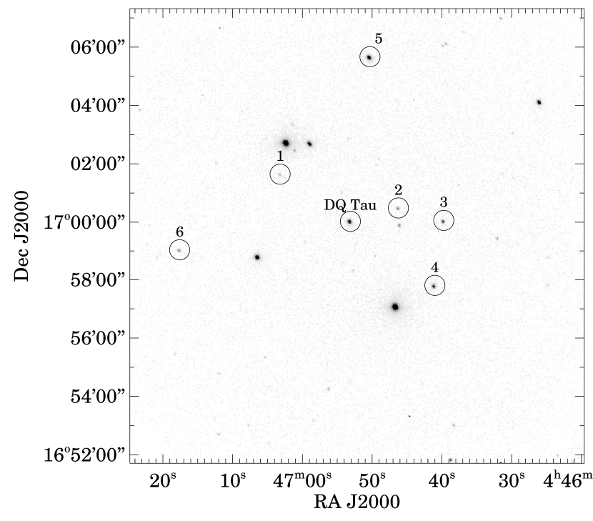
Figure 9: The comparison stars used to derive the differential photometry for DQ Tau. The figure shows the complete 15.6${}^{\prime}\,{\times}\,$15.6^′ field of view for the Wellesley 0.6-meter telescope. This I-band image was obtained on 2008 December 25.

In order to convert instrumental magnitudes to the standard system, we observed the equatorial standard stars HD 65079 and GD 50 at different airmasses on 2008 December 25 and 28 at Wellesley. Atmospheric extinction coefficients and zero-magnitude offsets were calculated by comparing our instrumental magnitudes above the atmosphere to the standard values in the literature (Menzies et al. 1991; Landolt 1992). These corrections were then applied for six comparison stars in the vicinity of DQ Tau, observed on the same two nights. The comparison stars are identified in a sample optical image in the online material (see Fig. 9), and their final absolute magnitudes are provided in Table 5 online. We estimate a photometric uncertainty of about 0.5 mag. Two of our comparison stars (#4 and #5) were included in the Droege et al. (2007) study, and they have a very low Welch-Stetson variability index, confirming that they are sufficiently constant to be used as comparison stars. The absolute magnitudes that we derived for these two comparison stars agree to within 0.2 mag with the catalog values (Droege et al. 2007). Since all six comparison stars are bluer than DQ Tau, we did not attempt to determine a color term, but simply averaged the differential magnitudes obtained with the six comparison stars. Using this method, we estimate that the precision of the repeatability is 0.05 mag, meaning that we take changes in the light curve larger than the precision value to be real.

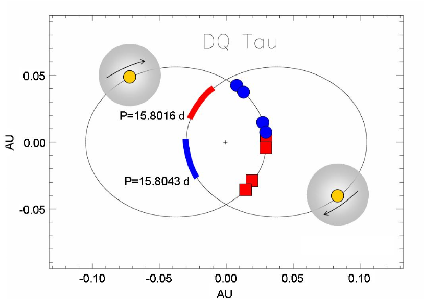
Figure 2: The effect of the assumed orbital period on the estimated timing of the flares. A cross indicates the barycenter of the binary system while ellipses trace out the retrograde motions of the binary components. Along one ellipse, we highlight the orbital segment covered by the observations, as determined for each period. On the other ellipse, we indicate the point in the orbit when the trigger event is presumed to have occurred for each periastron monitored. We use blue circles for the Mathieu et al. (1997) value of 15.8043 days and red squares for the 15.8016-day period from Huerta et al. (2005). Set at a greater distance from periastron, we indicate DQ Tau A and DQ Tau B drawn to scale (R_⋆ = 1.6 R_⊙) with an accompanying magnetosphere of R = 5 R_⋆.

3 Results and analysis

3.1 Millimeter flare properties

For all millimeter tracks, DQ Tau remains unresolved at all times. Given a distance of 140 pc to the Taurus star-forming region (Kenyon et al. 1994), and a maximum instrument resolution of 0.7^′′ (Table 3), we can already constrain the millimeter emission to a region within 100 AU of the binary. The corresponding light curves and track statistics retrieved from the data reduction are plotted in Fig. 1 and summarized in Table 3. In addition, the individual Julian dates and flux values comprising each light curve are provided in Tables 6–10 online.

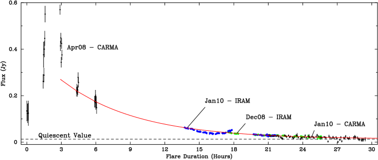
Figure 3: The 3 mm band light curves are shifted along a common exponential decay curve with an e-folding time of 6.55 hours. For a zoomed-in version of how well the model fits the decays from Dec08 and Jan10, please refer back to Fig. 1. Based on this fit, we loosely establish the upper limit for an average flare duration to be 30 hours.

In the follow-up observing campaigns, we report confirmed elevated millimeter activity showing a clear decline in brightness with time on 2008 December 28 and on 2010 January 11 (hereafter abbreviated as the ‘Dec08’ and ‘Jan10’ periastron events). The activity supports a periodic behavior linked to the binary orbit. However, the variable nature of the magnetospheres, and in particular their tendency to fluctuate in size, also means that the exact timing of a flare is understandably difficult to predict. On 2009 March 17 (hereafter the ‘Mar09’ event) the light curve is quiescent until the last hour of the track when it increases in brightness to 1.5 times its quiescent value. At this point the source was nearing an elevation of just 15^∘, but since the gain calibrator remains at a reliable elevation, we might only expect a loss in source flux at such a low elevation. Therefore, we conclude that the brightening is a real effect and very likely the start of a flare, occurring a mere 6 hours later than we had predicted. It is certainly unlikely in a (magnetospheric) collision scenario that a significant flare could have occurred much earlier in the orbit when the stars are at a much greater separation. In this regard, the incompletely-observed onset could raise questions as to whether the millimeter flares share more in common with the optical brightenings, which have been shown to occur for most but not all periastron encounters (Mathieu et al. 1997).

To calculate the timing of each periastron event, we used the orbital parameters determined by Mathieu et al. (1997), specifically JD₀ = 2 449 582.54 $\pm$ 0.05 and $P$ = 15.8043 $\pm$ 0.0024 days. We note that a revised period has since been published by Huerta et al. (2005), where their more recent data suggests a shortening of $P$ to 15.8016 $\pm$ ${}^{0.002}_{0.006}$. This new period is within the initial error bars of the original, confirming the overall robustness of the orbital period, but the newer value is itself less precise. In Fig. 2 we illustrate how the assumed period affects the perceived timing of the flares within the orbit. Along one orbital path, we highlight the section that would correspond to our millimeter observations for each proposed period. The original period indicates that our observed events occur as the stars approach one another, whereas the revised period consistently places the observed activity at or after periastron. Due to the irregular nature of the magnetic fields, our data cannot differentiate between the correctness of one period over the other. And, in fact, flares both before and after periastron are possible, as we discuss in Sect. 4.3. Instead, we suspect that the most energetic events in this system are more likely to occur during the initial interaction, upon approach. Therefore, the orbital phases reported in Table 3—and throughout this paper—are calculated using the original period of $P$ = 15.8043 days.

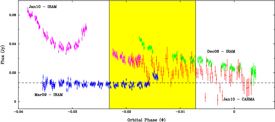
Figure 4: A plot of the 3 mm band fluxes versus orbital phase, illustrating how the activity shifts around slightly in the orbit. An orbital phase $\Phi$ of 0 defines periastron. The shaded region indicates the phase coverage for the initial Apr08 flare and is equivalent to 8 hours. During the Dec08 and Jan10 follow-up observations, the flare occurred earlier in the orbit, while the Mar09 follow-up observation may have occurred later, but not earlier (at least not within the previous day).

In none of the follow-up observations do we succeed in capturing a single flare in its entirety. The longest continuous coverage is for 18 hours in January 2010 when IRAM, CARMA, and SMA observed DQ Tau in succession. The source remains in an elevated flux state at 90–95 GHz for the duration of this joint observation, but appears quiescent (within the noise levels) at 238 GHz. The Jan10-SMA track-averaged flux at 238 GHz is 97 mJy versus 13 mJy at 90 GHz during the quiescent portion of the Mar09-IRAM track. Together, these flux values define a millimeter spectral index $\alpha$ of $\sim$2, which is consistent with thermal emission from an optically thick disk. During the Jan10 flare, however, the starting flux measurements at SMA (97 mJy) and CARMA (30 mJy) document an $\alpha$ of 1.2, providing strong evidence for the presence of non-thermal emission (see Sect. 4.1).

Since DQ Tau is only above the horizon for 8–10 hours at any given site, each observation date covers an even smaller window of the recurring activity. However, the separate flare events from Dec08 and Jan10 exhibit very similar flux levels and large-scale decay profiles. When we independently fit an exponential curve to the decaying flux intensities from both dates (shown atop the data in Fig. 1), we found identical e-folding times of 6.55 hours. (We will return to their sub-structure shortly.) If the same e-folding time holds for more (or even all) flares, then each individual observation could loosely correspond to a different portion of the same decay curve. Thus by shifting the separate flare profiles with respect to one another, as is shown in Fig. 3, we can attempt to re-construct an “average” flare profile. We can even place constraints on the duration of an outburst if we know the peak flux for each flare. With only one peak flux for reference, we extrapolate the exponential fit back through the last flux value from the original Apr08 event. In this way, we estimate a flare duration of approximately 30 hours.

This calculation for the flare duration should be regarded with some caution, and taken as an upper limit only in most cases. First, the initial decay slope following the strongest outburst in Apr08 is much steeper than the long steady decays observed in Dec08 and Jan10. As a result, a disjointed superposition of two decay profiles, rooted in two separate energy dissipating processes, may prove a better model and ultimately shorten the flare length. (In Sect. 4.1 we discuss these loss mechanisms further.) Secondly, the assumption of a similar peak flare intensity from one periastron to the next is one property where we lack sufficient millimeter data. To reinforce this idea, simultaneous X-ray observations during the Jan10 event indicate only a relatively weak X-ray flare; one that is hardly powerful enough to expect a radio counterpart with a peak flux as explosive as the original Apr08 event (Getman et al., submitted). Finally, it is improbable that the peak fluxes are identical given the complicated nature of the magnetic fields, the dependence on the ionized particle reservoir, the magnetic energy released during an event, as well as the diversity that we can already document in the decay profiles. However, this method provides some necessary constraints to characterize the millimeter activity. In turn, for a 15.8043-day period assuming one 30-hour flare per orbit, we suspect that DQ Tau could spend up to 8% of its time exhibiting excess flux that is unrelated to the thermal continuum emission from its circumbinary disk.

If we take this analysis one step further, we can use the relative offsets from Fig. 3 (e.g. $\sim$13.5 hours for Jan10 and $\sim$17.5 hours for Dec08) to estimate the orbital phase $\Phi$ for the initial outburst event (or $t$ = $0$). These are the orbital points indicated along the second ellipse in Fig. 2, and in numerical form in Table 3 (Column 10) where $\Phi$ = 0.0,1.0 defines periastron. If we now continue to assume that the Mar09 track signals the start of a large flare, then the Jan10 and Mar09 flares exhibit the largest separation in orbital phase, suggesting an outburst event window of $\sim$22 hours (or $\sim$6% of the orbital phase). Physically, this window encompasses a stellar separation of 8–13 R_⋆ and is equivalent to roughly one-third the time needed for the stars to swap positions about the system center ($\sim$2.8 days; Basri et al. 2010). In Fig. 4 we plot the millimeter flux versus the orbital phase for all tracks, to show how the elevated activity shifts back and forth in the orbit, yet consistently occurs in the day before periastron ($-$0.06 $<$ $\Phi$ $<$ 0.0). Together, the estimated flare duration plus the variable orbital timing for the outburst event, define a window of breadth 52 hours (or $\sim$2.2 days) when the millimeter flux may exceed the thermal quiescent value.

While the similarity in the large-scale decay times for both Dec08 and Jan10 is quite striking, the curves show sub-structure that is rather diverse. During the Apr08 and Dec08 events, we captured a smooth exponential decay, exhibiting only very small variations in the measured flux values. The Jan10 light curve, however, features a sharp break in the general decay profile one hour into the observation, initially dropping more rapidly before giving rise to a milder secondary peak, and then finally resuming the original decay profile. (We note that the 2-hour gap in the data during this time was the result of an antenna error, and that the observations quickly resumed without the faulty antenna.) We interpret the sub-structure from Jan10 to be due to a secondary event, occurring about 15 hours after the estimate for the initial outburst, and involving a smaller energy release than the preceding flare. In fact, this occurrence of successive events suggests that a series of (probably less powerful) flares can take place, possibly in lieu of one giant outburst.

The Jan10 multiple-peak observation, which occurred earliest in the orbit, was presumably less powerful (drawing on the X-ray analysis) than the original Apr08 outburst, which occurred closer to periastron (Fig. 4). While we lack information on the full millimeter light curves to make a conclusive statement, we note that a similar inverse relationship between flare intensity and peak timing was documented toward V773 Tau A (Massi et al. 2008). One caveat to the assumption of a lower peak flux is that it shortens our estimate for the flare duration, and thus the phase of $t$ = 0. On the other hand, a superposition of multiple flares spaced slightly apart in time can lead to both shortened or extended periods of activity, which can only be better characterized by a larger monitoring program.

Additional small-scale variations in the total flux density are likely due to atmospheric and instrumental effects. Larger systematic changes can help us test for strong linear polarization using the new, dual linear polarization receivers available at IRAM PdBI in combination with Earth rotation polarimetry, as described in Trippe et al. (2010). There the authors show how the difference in flux between the two orthogonal polarization feeds, divided by their sum, changes in a systematic way when a linearly polarized source transits. Unfortunately, this technique and the instrumentation available does not allow us to constrain the presence or amount of circularly polarized light. Using this method in the absence of detecting all 4 Stokes parameters, we determine 3$\sigma$ upper limits of 4.65% and 7.60% for the linear polarization during the flare decay phases from Dec08 and Jan10, respectively. During the quiescent Mar09 track, our upper limit is 8.15%. In Sect. 4.2, we discuss the implications of the linear polarization fractions for the proposed picture and the emission mechanism.

3.2 Coincident optical brightenings

DQ Tau is perhaps best known as the first system to be studied in terms of pulsed accretion flows to explain its optical variability near periastron. The binary has therefore been characterized extensively at optical and near-infrared wavelengths, using both photometric and spectroscopic observations (Herbst et al. 1994; Mathieu et al. 1997; Basri et al. 1997; Huerta et al. 2005; Boden et al. 2009). In Table 4 online, we provide the photometry results from our own observing campaigns in December 2008, January 2009, and January 2010. We note here that when we compare the Teide and the Wellesley data obtained on 2008 December 28—the only night for which the two telescope observations overlap in time—we find a slight offset between the magnitudes obtained with the two telescopes, which is within the uncertainties stated in Sect. 2.2. Consistency can be achieved by subtracting 0.08 mag from the Wellesley V magnitudes and 0.05 mag from the Wellesley R and I magnitudes. We emphasize that, while the online photometry table does contain the original unshifted magnitudes per telescope, we have shifted these data accordingly for all plots displayed here for the purpose of our analysis and the discussion that follows.

In Fig. 5 we plot our photometry values first as a function of the orbital phase $\Phi$ for all three optical filters. In the optical V band, the source is known to brighten by $\approx$0.5 mag within an orbital phase window of breadth 0.30 (or $\sim$5 days), centered on a phase of $-$0.1 (or about 1.6 days before closest approach). The V filter always shows the greatest amplitude change, but the variations are mirrored in all filters. This “bluening” effect caused by increased veiling is just one of the expected results from the ongoing accretion processes (Basri et al. 1997). We also observe the same 5-day activity window for the optical brightenings, which is a window 2.3 times broader than the millimeter window documented thus far. Our photometry results are indeed consistent with previous studies (see Mathieu et al. 1997, Fig. 4). One unique feature in our data, however, is the apparent double-peaked nature of these most recent brightenings, indicating a clustering of events around two phases. We caution against over-interpreting this effect since the data set is sparsely-sampled, covers only 4 periastron encounters, and is heavily dominated by the Dec08 event in particular (see Fig. 6). Nevertheless, the behavior is intriguing given the emerging picture for star-star reconnection events, and we will return breifly to this result in Sect. 4.4.

Figure 5: The VRI photometry values wrapped with the 15.8043-day orbital period for DQ Tau, where $\Phi$ = $\pm$0.5 indicates apoastron and $\Phi$ = 0 is periastron. The optical brightenings occur within a 5-day window near periastron, as was first shown by Mathieu et al. (1997). Filled symbols represent data taken with the Teide IAC-80 telescope and unfilled data points are from the Wellesley telescope. Horizontal lines indicate the quiescent absolute magnitude per filter.

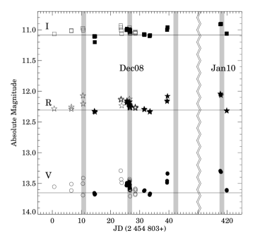
Figure 6: A plot of the VRI photometry values for the Julian dates from December 2008 through January 2009, as well as January 2010. The shaded columns indicate periastron events. The source brightens irregularly prior to all four newly documented periastron encounters.

In Fig. 6 we unwrap the optical data and show the results of continuous monitoring from December 2008 to January 2009, as well as several measurements from January 2010. We indicate the absolute magnitude versus Julian Day, where the bi-weekly periastron events are indicated with a shaded column. The source is found to increase in brightness in the days leading up to each of the 4 periastron encounters that we monitored, even though optical brightenings were not seen for all encounters monitored by Mathieu et al. (1997). Of particular interest are the second and fourth shaded columns in Fig. 6 (at JD = 2 454 829 and 2 455 221, respectively), which represent the dates for the Dec08 and Jan10 observations, confirming coincident optical and millimeter activity on each date. No optical data is available for Mar09 and Apr08, corresponding to a time of year when the source is below the horizon at night.

The Dec08 event offers the most extensive simultaneous optical coverage. In Fig. 7 we show how the optical and millimeter outbursts are related in time. On the night before the millimeter track, the optical light curve begins to brighten. During the millimeter decay the following night, the optical light curve decreases in step with the millimeter flare. This brightening and subsequent decay shows that the optical activity is not only coincident in time, but also in duration, with the average millimeter profile.

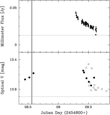
Figure 7: A plot showing the simultaneous millimeter (upper panel) and optical (lower panel) coverage for the Dec08 periastron encounter. A thin gray horizontal line in each panel represents the quiescent value. The optical light curve begins to brighten the night before, returning to quiescence in time with the millimeter decay. We indicate with a thick vertical line $t$ = 0 for the estimated time of the trigger event, assuming an average 30-hour flare. In this case, the optical activity appears coincident in both time and duration with the millimeter activity.

4 Discussion

4.1 Signatures of synchrotron emission

The millimeter emission is almost certainly non-thermal in origin given the sudden flare onset and the fast decay time. In the solar analogy, it is generally accepted that this type of extraneous emission from high-energy electrons is synchrotron in origin, and that emission at shorter millimeter wavelengths results from the most energetic (MeV) electrons (Silva et al. 2007). We eliminate non-relativistic cyclotron radiation as a primary emission process because the magnetic field strength required to produce cyclotron emission ($B=2\pi\,m_{e}/q$) at 90 GHz is 30 kG; increasing to 80 kG at 238 GHz. These values are much larger than the 1–6 kG surface field strengths expected (or measured) for TTSs (Guenther et al. 1999; Johns-Krull 2007). Instead, the electron population probed by our observations must possess mildly to highly relativistic properties, representing gyro-synchrotron and synchrotron radiation mechanisms, respectively.

In this subsection, we follow closely an analysis similar to that presented in Massi et al. (2006) for synchrotron emission from the interacting coronae of V773 Tau A. We model the outer (large-scale) structure of the DQ Tau magnetospheres to be well-ordered dipoles and we take the magnetic axes to be aligned parallel to the rotational axes, assumptions that are consistent with recent 3D extrapolations of the coronal field topology for several young stars (Gregory et al. 2008). We do assume that the rotational axes are both aligned perpendicular to the plane of the system, although we acknowledge that, in rare cases, large misalignments have been documented around a short-period binary (Albrecht et al. 2009). We know that the DQ Tau system is inclined 157^∘ to the line-of-sight (Boden et al. 2009), and we presume that the reconnection events occur in the equatorial region between the two stars. For a synchrotron spectrum, Ginzburg & Syrovatskii (1965) showed that the maximum spectral frequency (in Hz) is proportional to the perpendicular component of the magnetic field $B_{\perp}$ (in Gauss) and the Lorentz factor $\gamma$ squared:

$$\nu_{\rm max}=1.2\times 10^{6}B_{\perp}\gamma^{2}$$ (1)

Since millimeter brightenings have been consistently observed near 90 GHz, we conservatively assume this value for $\nu_{max}$, meaning that there must be an electron population whose relativistic properties in vacuum satisfy the following relation:

$$B\gamma^{2}=8.1\times 10^{4}$$ (2)

Using an average surface field strength of 3 kG, we can calculate the Lorentz factor for several relevant distances, including: half the minimum binary separation ($d$ = 4 R_⋆, $B$ = 47 G, $\gamma$ = 42); the minimum binary separation ($d$ = 8 R_⋆, $B$ = 6 G, $\gamma$ = 116); and the distance to the inner rim of the circumbinary disk in the case of a star-disk interaction ($d$ = 54 R_⋆, $B$ = 0.02 G, $\gamma$ = 2012). All scenarios give rise to highly relativistic ($\gamma$ $\gg$ 1) particles, and thus synchrotron emission. For gyro-synchrotron ($\gamma$ $\approx$ 5) emission only, contributions would be restricted to stellar heights of 0.3–1.5 R_⋆ and most likely indicate single-star magnetic activity that is independent of the orbital period.

Due to the nature of synchrotron emission and the local magnetized environment, competition between radiation and collisional losses represent the largest impactors on the exponential decays that characterize our millimeter light curves. We start with the following expression for synchrotron radiation losses (in hours) for a well-ordered field (Blumenthal & Gould 1970):

$$\tau_{s}=\frac{1.6\times 10^{5}}{B^{2}\gamma}$$ (3)

In combination with Eq. 2, we can solve for the two unknowns when we use a synchrotron decay time $\tau_{s}$ equal to the e-folding time of 6.55 hours. We find $B$ = 19 G and $\gamma$ = 65. For the full range of dipolar field strengths expected for a TTS (1–6 kG), this result localizes the main emitting region to a stellar height of 3.7–6.8 R_⋆. We note that the values are centered around the theoretical size for a T Tauri magnetosphere. They are also consistent with a site located halfway between the two stars for the separation distances at the times of outburst ($\sim$8–13 R_⋆ as determined in Sect. 4). This range compares well with the coronae loop size infered by Getman et al. (2010, submitted) to explain the X-ray activity, which derives from a related process but a separate electron population. Alternately, if significant emission were to be observed near a $v_{\rm max}$ of 238 GHz, then the stellar height range identified would increase (unless a weaker stellar magnetic field or a faster decay time at the higher frequency were to compensate).

Next we constrain the maximum density of the electrons spiraling along the field lines by calculating what the thermal Coloumb collisional losses (in hours) would need to be in order to shorten the observed decay time. We use (Petrosian 1985; Massi et al. 2006):

$$\tau_{c}=4.16\times 10^{8}\frac{\gamma}{n_{e}}$$ (4)

to derive a maximum electron density of $n_{e}$ $\leq$ 3.7 $\times$ 10⁹ cm^-3. A final check of the condition (Ginzburg & Syrovatskii 1965):

$$\nu\gg\nu_{c}\simeq 20\frac{n_{e}}{B_{\perp}}$$ (5)

confirms that the vacuum approximation used throughout these calculations is valid in the case of the DQ Tau magnetospheres as accelerated electrons spiral down from large stellar heights.

The fact that synchrotron losses explain the light curve profiles well implies that the relativistic electron reservoir is sufficiently confined, or trapped, within the global magnetic structure. One of the key conclusions from the Massi et al. (2006) model for V773 Tau A was that electrons must leak out at magnetic mirror points in order to diffuse the synchrotron emission fast enough to achieve their observed e-folding time of 2.31 hours. While evoking this effect is unnecessary late in our own flare timeline, we note that a much steeper decay is present in the initial hours of the Apr08 flare (refer to Fig. 3). It is possible that a similar leakage of electrons could also occur in the DQ Tau system shortly after the initial outburst, or perhaps as (accreting) charged particles are initially expelled from the system in a manner similar to a coronal mass ejection in the Sun. Or perhaps a more probable scenario is that the Apr08 decay, like the Jan10 dip, is the result of the Neupert effect and the thick-target mechanism (see Getman et al., submitted). We do rule out several geometrical effects, including an eclipse due to rotation, because the stellar rotational periods have been determined to be $\sim$3 days (see Basri et al. 1997), while the maximum deviation from the decay profile lasts at most 5.5 hours. In the end, the geometry-independent, natural synchrotron decay process (vs. particle loss or leakage) as the primary loss mechanism agrees much better with the persistent, large-scale decay profiles observed from one flare to the next.

4.2 De-polarization effects

Synchrotron emission predicts a high fraction of linearly polarized light, up to 70% in a well-ordered magnetic field, although it is rarely observed to be maximally polarized (e.g. Sokoloff et al. 1998; Trippe et al. 2010). Our own observations limit the polarization fraction toward DQ Tau to $<$ 5–8%. The measurements sample both a quiescent state as well as two flare decays, and do not rule out the presence of linear polarization altogether. Instead, we explore de-polarization effects that can reduce the observed polarization fraction.

Polarized light originates in regions where the magnetic field lines are stable, well-ordered, of a single orientation, and of a single magnetic polarity. Since the plane of polarization is perpendicular to the magnetic field, a tangled field unresolved by the telescope beam leads to beam averaging of the different polarization vectors, effectively de-polarizing the light. In Sect. 3 our resolution constrained the emission to a region 100 AU from the binary, an area that encompasses the two independent magnetospheres. Within this view, dipolar magnetospheric field lines on one star begin in its northern magnetic hemisphere and end in its southern magnetic hemisphere, effectively doubling back 180^∘ in direction within the telescope beam. In addition, the field polarity of one star may be reversed with respect to the companion’s. In fact, we show in Sect. 4.3 how this is probably the case for DQ Tau. Therefore, the geometry of the field lines where the accelerated electrons are trapped has a very important impact on the net polarization observed, and any positive polarization detections may favor emitting regions at larger stellar heights where the magnetic field is simpler and well-ordered, since higher-order field components typically fall off more quickly (Gregory et al. 2008).

Nevertheless, linear polarization has been measured toward V773 Tau A, the only other known PMS binary to exhibit evidence of star-star magnetic interactions. Phillips et al. (1996) detected a significant fractional polarization of 2% at cm wavelengths. However, follow-up polarization observations of V773 Tau A during periods of millimeter activity produced only non-detections at both millimeter and centimeter wavelengths (Massi et al. 2008). Generally, polarization is considerably weakened toward the radio end of the spectrum, mainly due to Faraday rotation effects (Ginzburg & Syrovatskii 1965). The effect occurs as linearly polarized light passes through a dense, magnetized medium causing the polarization angle $\theta$ to rotate by an angle equal to $RM$ $\lambda^{2}$ where $RM$ is the rotation measure (in rad m^-2) defined as:

$$RM=8.1\times 10^{5}\int n_{e}B_{||}\,ds$$ (6)

Here $n_{e}$ is the electron density (in cm^-3), $B$ is the longitudinal magnetic field strength (in Gauss), and $ds$ is the line-of-sight path length (in pc) through the magnetized medium. When the rotation measure is larger than $\sim$10⁵ rad m^-2 at 3.3 mm, Faraday de-polarization is complete in a homogeneous medium. This is equivalent to a rotation angle of 90^∘, although rotation angles as small as 5–10^∘ (or $RM$ $\approx$ 10⁴) can also be sufficiently effective, depending on the method detection threshold and the intrinsic polarization fraction.

Faraday rotation can occur in any magnetized region along the line-of-sight, including the interstellar medium and the Earth’s ionosphere. However, the synchrotron emission from DQ Tau predicts large electron densities (10⁹ cm^-3) and strong magnetic fields (3 orders of magnitude greater than the Sun’s field), suggesting that the emitting region itself has the potential for the greatest de-polarization effect. To test this possibility, we model electrons trapped in the magnetospheres with a shell of outer radius 5 R_⋆ and a thickness of 1 R_⋆. The electron density is set to the maximum determined from synchrotron losses and taken to be constant throughout the shell. The magnetic field strength is modeled as a dipole with a surface field strength of 3 kG. In this scenario, we derive an $RM$ of $\sim$ 10⁹ rad m^-2, which undoubtably results in complete de-polarization of the synchrotron emission.

Conceding that this initial calculation may represent a case of maximized extremes, we can do the same calculation for an electron density of 10³ cm^-3 (essentially an upper limit in a molecular cloud of typically 10³ molecules per cm^-3), a shell thickness of 0.1 R_⋆ (equivalently the size of the stellar corona), and a reduced dipole field of surface strength 1 kG. We find an $RM$ value of $\sim$10², which is below the cutoff for complete de-polarization. To recover a factor 100 in the $RM$, we determine that a minimum density of 10⁵–10⁶ cm^-3 is needed to sufficiently de-polarize the millimeter emission. These values are representative of the density in the uppermost layers of the circumbinary disk, and for a source experiencing (simultaneous) accretion, should be easily obtained, at least along the accretion streams. Therefore, we predict that the synchrotron source is sufficiently self de-polarizing to result in the complete absence of linear polarization for most geometries.

4.3 Orientation and topology of the magnetospheres

A dipole representation of the magnetospheres remains an adequate and consistent model for the analysis, and is the simplest valid structure. When we illustrate the corresponding field lines in Fig. 8, there are, in fact, two scenarios for the timing of the reconnection events: during both the approach and separation phases. During approach, the field lines are oppositely-directed in the equatorial region and undergo compression as the stars approach periastron and the fields repel one another. At the vertical boundary layer between the two magnetospheres, where their merging plasma flows and induced electrical currents resist one another, reconnection can occur. The two magnetospheres join together via shared field lines that begin on one star and now end on the other. During separation, the global field is split into two closed magnetospheres through stretching, and thus compression of the lines near the orbital plane of the system. Both scenarios release energy into the surrounding region, accelerating charged particles at large stellar heights down along the magnetospheric field lines toward the star, which is when both scenarios produce (gyro-)synchrotron radiation in a relatively indistinguishable manner.

In the figure, we point out that the magnetic axes are drawn with an inverse alignment. In an aligned system, trying to connect the field lines from the magnetic north of one star to the magnetic south of the other results in crossed lines, which would quickly reconnect, reverting back to two dipole structures. Thus, in this arrangement, the global magnetic topology is strictly maintained. The magnetic density still increases upon approach, building up magnetic energy stores, but the boundary layer between the two magnetospheres is imperceptable to the local plasma and electrical currents. There is far less resistance to the re-arrangement (e.g. compression) of the field lines, as compared to the reverse case, and reconnection is not favored as a result.

Assuming parallel rotational axes perpendicular to the orbital plane, and that magnetic axes tend to be aligned with the rotational axis in many astrophysical bodies (as we justified in Sect. 4.1), the two magnetospheres should be either aligned (0^∘) or inversely aligned (180^∘). Undoubtedly, in this bimodal interpretation, the DQ Tau magnetospheres therefore must be inversely aligned to produce the flares observed. This does present an interesting consequence for the millimeter flares if one of the magnetic fields were to flip, as the Sun’s field is prone to do once every 11 years; an effect that has been observed toward other PMS stars with short rotation periods (Donati et al. 2008; Fares et al. 2009; Petit et al. 2009). In this case, if the magnetospheres are the principle mechanism for the flaring phenomenon, and if their magnetic axes are indeed more or less aligned, then we could expect on-and-off periods of millimeter activity near periastron.

Finally, there are the oblique cases when the field lines forced together are not similary- or oppositely-directed, but rather cross at an intermediate angle. This can occur if the magnetic axes are tilted with respect to one another. The occurrence of reconnection then depends on the orientation angle, the field strengths, the merging systems of flux, and the resistivity to the topological changes caused by the induced currents. Consequently, one conclusion to make is that the DQ Tau magnetospheres must be misaligned by a significant angle to produce reconnection events and their associated millimeter flares.

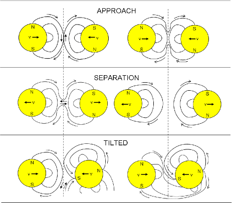
Figure 8: An illustration of the scenarios for reconnection events in the DQ Tau binary system during approach (upper panel) and separation (middle panel). In the lower panel, we show a variation to the upper panel if the magnetic axes are tilted with respect to one another. This misalignment can also occur into or out of the page, causing field lines to cross at intermediate angles that may or may not result in reconnection. Similar variations to the middle panel are also possible.

The other possibility is that the magnetospheres are poorly modeled by a dipolar field between 4–7 R_⋆ (or 6.4–12 R_⊙), which is the half-distance separation of the two stars during the observed flares. In the Sun, the dipole component dominates beyond 2.5 R_⊙, but in PMS stars the relative strengths of the field components can vary widely (Gregory et al. 2008). For example, toward the TTS V2129 Oph the octopole component was found to dominate out to 6.7 R_⋆ (Donati et al. 2007), providing ample opportunity in a binary system for opposite-polarity regions to interact and reconnect at large separations. Other deviations include the winding up of the field lines as the stars rotate faster in the equatorial region. This effect is amplified with respect to the Sun given that these stars rotate 10 times faster. However, we expect that the winding effect should act to slow the rotation in an aligned system, and encourage reconnection as usual in an inversely aligned system.

The accretion streams can also produce local changes in the field lines, including compression and ordering of the magnetosphere during episodic events. It is unclear what should be expected from a collision of two streams with equivalent mass accretion rates, but it may mirror the complex and unstable merging of two stellar jets, as modeled by Mundt et al. (2010). There the authors predict that, as the outflows in a binary system combine at large stellar distances, reconnection events should result near the intersection point. Finally, the trigger might simply be a inter-coronal interaction very similar to the Massi et al. (2006, 2008) scenario for V773 Tau A. There the extended magnetic structure was imaged at a stellar height of 48 R_⊙. Thus, if similarly extended structure were present on the stars in the DQ Tau system, then flares could result at any time in the orbit. Although currently, all observations outside our defined outburst event window report quiescent fluxes (Salter et al. 2008; Guilloteau et al., in prep), suggesting that this is not the most robust description for the current observations. Of course, we cannot rule out millimeter contributions from a combination of scenarios.

4.4 Optical emission mechanisms

The coincident timing and duration of the optical and millimeter brightenings in Fig. 7 is intriguing, but the physical interpretation remains a challenge. While we have presented evidence that the millimeter emission arises from recurring star-star reconnection events, the origin of the optical emission can be rooted in both dynamical processes (e.g. accretion pulses due to the binary motions) and magnetospheric processes (e.g. reconnection events). In this section, we consider whether both processes are required to explain the optical behavior.

Flare models often include an optical emission component due to the heating and ionization of the chromospheric plasma where the non-thermal electron population spirals down into the stellar atmosphere, typically at a magnetic field footprint (Haisch et al. 1991; Güdel 2002). In this picture, an optical brightening is normally expected to accompany the millimeter activity, just like we currently observe. It is thus tempting to recall the double-peaked nature of the optical brightenings in Fig. 5, in light of our scenario for interacting magnetospheres, which predicts two reconnection events associated with first the joining and then the separation of the magnetospheres. The data presented in Mathieu et al. (1997) do not preclude optical brightenings clustered around two separate phases, spaced apart in time by roughly 3 days ($\Delta$$\Phi$ $\approx$ 0.2). In addition, Mathieu et al. (1997) also determined that enough magnetic energy is available in the outer magnetospheres to power the average DQ Tau optical brightening, even though the authors questioned whether the field could regenerate itself on a bi-weekly basis. Although our millimeter observations do not cover back-to-back periastron encounters, our consistent flare detection rate suggests that reconnection occurs during most, if not all, orbits. However, it remains unclear whether this result favors a quick and efficient regeneration of the field or an alternative mechanism to drive the optical brightenings.

Instead, other observational results favor optical brightenings linked to independent accretion processes. Mathieu et al. (1997) noted first that the optical brightenings occur quite far from periastron to be the result of reconnection, as well as the spectral bluenings seem to disagree with the optical flat-spectrum (or “white-light”) continuum enhancements that more typically accompany flares (e.g. Hudson et al. 1992; Güdel et al. 2004). Likewise, some of the DQ Tau optical brightenings appear to last continuously for up to 4 days (Fig. 2 of Mathieu et al. 1997), much longer than an “average” millimeter flare. In Sect. 3.2 we determined that the observed millimeter activity window was 2.3 times smaller than the optical, but we concede that our phase sampling was intentionally restricted to the 24-hour period before periastron, and therefore we lack a detailed overview of the millimeter perspective at larger separations. This fact, combined with the Massi et al. (2008) evidence for interacting coronae at large ($\geq$30 R_⊙) stellar separations, suggest that only a prolonged multi-wavelength monitoring program over several cycles, and covering all orbital phases, can best characterize the relationship between the optical and millimeter activity, and the relevant dynamical and magnetospheric contributions.

In summary, it is not straight-forward to assign all of the elevated optical acitivity in this sytem to dynamically induced pulsed accretion events, particularly near periastron. Accretion appears to be ongoing at different levels throughout the orbit (Basri et al. 1997), with features that fit well the models by Artymowicz & Lubow (1996). Reconnection events, on the other hand, have only been documented near periastron thus far, but seem to always accompany an optical event. Thus, in all likelihood, reconnection and accretion processes are both contributing to the elevated optical activity, occurring simultaneously at periastron. To better ascertain the causal or co-dependent nature of the dynamical and magnetospheric processes, it is necessary to separate out the optical effects of each process.

5 Conclusions

We confirm periodic, elevated millimeter flux levels toward the DQ Tau PMS binary while monitoring 3 recent periastron encounters. The regularity of the flare timing is consistent with the proposed scenario for colliding magnetospheres within a day of closest approach, although the initiating event appears to vary within a 22-hour window corresponding to a binary separation of 8–13 R_⋆. The flaring mechanism can be explained by synchrotron emission from highly relativistic electrons accelerated near the reconnection site that begin to spiral down along the magnetospheres toward one or both stars. The main emission region is localized near a stellar height of 3.7–6.8 R_⋆, about halfway between the two stars at the time of an event. Synchrotron losses easily explain the similar (late-time) decay profiles, indicating both a well-confined electron population and a large stable magnetic structure from one event to the next. We estimate that the flares can last up to 30 hours per event, corresponding to 8% of the orbital period. In addition, multiple millimeter flares during a single periastron event have been observed within approximately 15 hours ($\Delta$$\Phi$ $\approx$ 0.04) of one another, with the secondary event being less powerful. The succession of events may correspond to first the merging and then the separation of the two magnetospheres, or simply to a trade-off between a slow sequential release of stored magnetic energy in lieu of one large outburst. A star-star magnetic reconnection event remains the simplest, most straight-forward interpretation in terms of the timing of the activity, the regularity of the occurrence, the magnetic field strengths implied, and the field sizes.

We measure an upper limit of 5–8% for the fractional linear polarization of the light, but we predict that both beam dilution and Faraday rotation in the DQ Tau system are probably sufficient to result in a net polarization of 0. We determine an upper limit of 3.7 $\times$ 10⁹ cm^-3 for the electron density in the field lines. However, if a non-zero polarization fraction is eventually detected, suggesting that Faraday rotation in particular is ineffective, then the upper limit for the emitting region must be revised to $\leq$ 10⁵–10⁶ cm^-3. Otherwise, another hinderence to the detection of polarization is the preferred orientation and topologies for the magnetic axes in order for reconnection to occur: either the dipoles are misaligned at a significant angle or else complex, higher-order magnetic structures are present at large stellar heights. In both cases, and for low-resolution observations specifically, reversed polarity footprints on each stellar surface will affect the measured polarization fraction. All things considered, the upper limit for the polarization in no way contradicts a synchrotron emission process.

The results of the simultaneous millimeter and optical monitoring reveal a particularly striking coincidence between the timing and duration of the multi-wavelength activity, but ultimately unravels little of the relationship between the dynamical and magnetospheric processes. We cannot distinguish between optical brightenings due to accretion events, reconnection processes, or a combination thereof. The current window for elevated millimeter activity is about 2.5 times smaller than the window for the optical brightenings. This preliminary statistic suggests that dynamically-induced accretion can occur independently; while each reconnection event thus far has been accompanied by an optical brightening that may, or may not, be associated with the accretion process only. Perhaps the only true test for the possible dependence of one process on the other, is to study similar binary systems where one effect is absent. We do suspect that this flaring phenomenon may be relevant to many similar T Tauri binary systems of high eccentricity, as we expect to see when new millimeter instrumentation reduces the time required for large, multi-epoch surveys.

Appendix A Optical data

Table 4: Optical observing log

JD+2450000	Obs.a	V [mag]	JD+2450000	Obs.	R [mag]	JD+2450000	Obs.	I [mag]
4803.640	W	13.64	4803.635	W	12.34	4803.661	W	11.12
4809.513	W	13.70	4809.517	W	12.34	4809.519	W	11.07
4809.534	W	13.59	4809.538	W	12.31	4809.540	W	11.07
4813.484	W	13.59	4813.489	W	12.13	4813.491	W	11.03
4813.506	W	13.77	4813.589	W	12.26	4813.591	W	11.06
4813.585	W	13.49	4817.416	T	12.32	4817.418	T	11.10
4817.414	T	13.66	4817.468	T	12.32	4817.469	T	11.11
4817.466	T	13.67	4817.503	T	12.33	4817.504	T	11.10
4817.501	T	13.67	4817.558	T	12.33	4817.560	T	11.20
4817.557	T	13.68	4817.682	T	12.34	4817.683	T	11.11
4817.680	T	13.67	4826.476	W	12.19	4826.472	W	10.99
4826.480	W	13.37	4826.640	W	12.18	4826.473	W	11.02
4826.632	W	13.51	4826.645	W	12.19	4826.651	W	11.06
4826.812	W	13.57	4826.805	W	12.29	4826.801	W	11.12
4828.451	T	13.53	4828.454	T	12.19	4828.455	T	11.00
4828.522	T	13.52	4828.523	T	12.17	4828.524	T	11.00
4828.591	T	13.49	4828.592	T	12.15	4828.593	T	10.98
4829.414	T	13.47	4829.415	T	12.17	4829.430	T	10.99
4829.427	T	13.49	4829.429	T	12.18	4829.459	W	11.05
4829.464	W	13.54	4829.462	W	12.18	4829.470	T	11.01
4829.468	T	13.53	4829.469	T	12.21	4829.471	W	11.02
4829.502	W	13.51	4829.479	W	12.31	4829.505	W	11.06
4829.506	T	13.55	4829.507	T	12.23	4829.508	T	11.02
4829.513	W	13.66	4829.508	W	12.29	4829.547	T	11.03
4829.521	W	13.64	4829.525	W	12.23	4829.548	W	11.06
4829.543	W	13.69	4829.527	W	12.28	4829.560	W	11.09
4829.544	T	13.57	4829.546	W	12.31	4829.591	W	11.09
4829.555	W	13.54	4829.546	T	12.24	4829.596	T	11.00
4829.585	W	13.67	4829.558	W	12.29	4829.604	W	11.08
4829.593	T	13.52	4829.589	W	12.32	4829.613	W	11.09
4829.599	W	13.65	4829.595	T	12.22	4829.635	W	11.08
4829.607	W	13.68	4829.603	W	12.32	4829.667	W	11.07
4829.629	W	13.69	4829.611	W	12.30	4829.707	W	11.06
4829.661	W	13.67	4829.633	W	12.30	4829.728	W	11.11
4829.702	W	13.79	4829.665	W	12.31	4829.756	W	11.11
4829.722	W	13.68	4829.726	W	12.32	4829.794	W	11.11
4829.798	W	13.69	4829.753	W	12.32	4831.440	W	11.10
4831.448	W	13.77	4829.796	W	12.32	4831.463	W	11.08
4831.468	W	13.75	4831.444	W	12.31	4831.479	W	11.11
4831.485	W	13.67	4831.465	W	12.33	4831.488	W	11.11
4831.493	W	13.70	4831.481	W	12.33	4831.502	W	11.10
4831.508	W	13.68	4831.489	W	12.31	4834.461	T	11.07
4834.454	T	13.62	4831.504	W	12.32	4834.536	T	11.08
4834.529	T	13.62	4834.458	T	12.29	4834.603	T	11.07
4834.596	T	13.67	4834.533	T	12.29	4834.661	T	11.08
4834.654	T	13.61	4834.600	T	12.30	4836.390	T	11.10
4836.396	T	13.69	4834.658	T	12.30	4836.398	T	11.10
4836.404	T	13.68	4836.393	T	12.34	4836.407	T	11.10
4836.413	T	13.69	4836.401	T	12.34	4836.519	T	11.09
4836.525	T	13.67	4836.410	T	12.34	4836.528	T	11.09
4836.534	T	13.66	4836.522	T	12.33	4836.536	T	11.09
4836.542	T	13.67	4836.530	T	12.33	4842.375	T	11.00
4842.369	T	13.49	4836.539	T	12.32	4842.387	T	11.00
4842.380	T	13.46	4842.372	T	12.17	4842.517	T	10.96
4842.510	T	13.34	4842.384	T	12.15	4842.527	T	10.96
4842.520	T	13.34	4842.513	T	12.08	5208.351	T	10.91
5208.360	T	13.30	4842.523	T	12.08	5208.474	T	10.91
5208.482	T	13.31	5208.357	T	12.04	5208.592	T	10.90
5208.597	T	13.31	5208.480	T	12.05	5210.532	T	11.06
5210.540	T	13.61	5208.596	T	12.07	5210.542	T	11.06
5210.550	T	13.61	5210.537	T	12.32	5210.553	T	11.06
5210.560	T	13.62	5210.547	T	12.31	5210.563	T	11.06
5210.571	T	13.62	5210.558	T	12.31
			5210.568	T	12.31
a To indicate the Teide Observatory IAC-80 telescope in the Canary Islands (Spain) we use a ‘T’, and for the
Wellesley 0.6-meter telescope at Wellesley College in Wellesley, Massachusetts (USA) we use a ‘W’.

Table 5: Comparison stars

Number	V [mag]	R [mag]	I [mag]
1	15.79	14.68	13.81
2	14.86	13.95	13.18
3	14.43	13.33	12.27
4	13.72	12.61	11.66
5	11.84	11.05	10.43
6	15.30	14.12	13.19

Appendix B Millimeter data

Table 6: Julian day, flux, and uncertainty values for the millimeter light curve on 2008 December 28-29, recorded at a central frequency of 90.0 GHz with the IRAM PdBI.

Julian Day	Flux	$\sigma$	Julian Day	Flux	$\sigma$	Julian Day	Flux	$\sigma$	Julian Day	Flux	$\sigma$
($+$2450000)	[mJy]	[mJy]	($+$2450000)	[mJy]	[mJy]	($+$2450000)	[mJy]	[mJy]	($+$2450000)	[mJy]	[mJy]
4829.290	44.4	1.0	4829.423	26.8	1.0	4829.538	25.5	1.0
4829.291	42.9	1.0	4829.424	28.9	1.0	4829.539	25.9	1.0
4829.293	42.8	1.0	4829.425	28.0	1.0	4829.540	22.8	1.1
4829.294	42.5	1.0	4829.438	30.4	1.0	4829.541	25.7	1.1
4829.295	42.5	1.0	4829.439	29.1	1.0	4829.542	24.2	1.1
4829.296	42.5	1.0	4829.440	27.5	1.0	4829.543	24.8	1.1
4829.297	43.1	1.0	4829.441	30.5	1.0	4829.554	22.5	1.1
4829.298	39.6	1.0	4829.443	27.0	1.0	4829.555	23.5	1.1
4829.299	39.9	1.0	4829.444	30.2	1.0	4829.557	23.3	1.1
4829.300	40.5	1.0	4829.445	26.6	1.0	4829.558	23.5	1.1
4829.301	40.3	1.0	4829.446	28.3	1.0	4829.559	25.5	1.1
4829.302	38.9	1.0	4829.447	28.7	1.0	4829.560	24.5	1.1
4829.303	36.9	1.0	4829.448	28.2	1.0	4829.561	23.1	1.1
4829.304	39.9	1.0	4829.449	29.7	1.0	4829.562	22.6	1.1
4829.305	37.4	1.0	4829.450	28.7	1.0	4829.563	23.7	1.1
4829.315	37.0	1.0	4829.451	27.5	1.0	4829.564	21.6	1.1
4829.316	36.9	1.0	4829.452	31.4	1.0	4829.565	23.3	1.1
4829.317	37.6	1.0	4829.453	25.5	1.0	4829.566	22.7	1.1
4829.318	36.3	1.0	4829.461	29.7	1.0	4829.567	22.2	1.1
4829.319	38.1	1.0	4829.462	27.9	1.0	4829.568	21.4	1.1
4829.320	37.6	1.0	4829.463	27.5	1.0	4829.569	22.8	1.1
4829.321	38.0	1.0	4829.464	30.6	1.0	4829.581	22.4	2.1
4829.322	36.9	1.0	4829.465	29.2	1.0	4829.582	23.0	2.1
4829.323	36.8	1.0	4829.466	25.3	1.0	4829.583	24.4	2.1
4829.324	37.6	1.0	4829.467	30.5	1.0	4829.584	20.3	2.1
4829.325	37.8	1.0	4829.468	27.0	1.0	4829.585	25.2	2.2
4829.326	37.2	1.0	4829.469	30.3	1.0	4829.586	24.1	2.2
4829.327	34.4	1.0	4829.470	28.0	1.0	4829.616	13.6	2.4
4829.328	34.0	1.0	4829.471	30.5	1.0	4829.617	20.7	2.5
4829.329	35.5	1.0	4829.472	28.9	1.0	4829.618	20.9	2.5
4829.386	31.2	1.0	4829.473	27.1	1.0	4829.619	21.0	2.5
4829.387	32.5	1.0	4829.474	28.2	1.0	4829.620	21.6	2.5
4829.388	29.6	1.0	4829.475	28.8	1.0	4829.622	19.5	2.5
4829.389	28.6	1.0	4829.488	28.1	1.0	4829.623	21.4	2.6
4829.391	31.6	1.0	4829.489	28.5	1.0	4829.624	24.2	2.6
4829.392	31.3	1.0	4829.490	28.9	1.0	4829.625	13.6	2.6
4829.393	31.0	1.0	4829.491	28.3	1.0	4829.626	18.8	2.6
4829.394	32.3	1.0	4829.492	28.0	1.0	4829.627	19.7	2.6
4829.395	31.5	1.0	4829.493	26.0	1.0	4829.628	22.6	2.7
4829.396	31.1	1.0	4829.494	25.0	1.0	4829.629	19.3	2.7
4829.397	32.0	1.0	4829.495	26.7	1.0	4829.630	21.7	2.7
4829.398	29.8	1.0	4829.496	27.6	1.0	4829.631	17.6	2.7
4829.399	33.1	1.0	4829.497	27.6	1.0
4829.400	32.0	1.0	4829.498	27.9	1.0
4829.401	34.4	1.0	4829.499	25.0	1.0
4829.410	32.1	1.0	4829.500	24.3	1.0
4829.411	30.2	1.0	4829.501	26.6	1.0
4829.412	29.7	1.0	4829.502	26.2	1.0
4829.413	29.3	1.0	4829.529	22.4	1.0
4829.414	30.7	1.0	4829.530	24.4	1.0
4829.415	30.4	1.0	4829.531	24.7	1.0
4829.416	30.7	1.0	4829.532	23.5	1.0
4829.417	30.2	1.0	4829.533	25.8	1.0
4829.418	29.2	1.0	4829.534	24.2	1.0
4829.420	30.2	1.0	4829.535	26.4	1.0
4829.421	27.9	1.0	4829.536	24.9	1.0
4829.422	28.6	1.0	4829.537	22.5	1.0

Table 7: Julian day, flux, and uncertainty values for the millimeter light curve on 2009 March 17, recorded at a central frequency of 90.0 GHz with the IRAM PdBI.

Julian Day	Flux	$\sigma$	Julian Day	Flux	$\sigma$	Julian Day	Flux	$\sigma$	Julian Day	Flux	$\sigma$
($+$2450000)	[mJy]	[mJy]	($+$2450000)	[mJy]	[mJy]	($+$2450000)	[mJy]	[mJy]	($+$2450000)	[mJy]	[mJy]
4908.028	12.8	1.7	4908.110	15.4	1.3	4908.199	12.5	0.9	4908.288	10.5	0.9
4908.029	9.4	1.7	4908.111	12.3	1.2	4908.200	9.4	0.9	4908.289	12.4	0.9
4908.030	17.0	1.7	4908.112	10.7	1.2	4908.201	12.4	0.9	4908.290	8.5	0.9
4908.031	12.1	1.7	4908.122	12.1	1.0	4908.202	11.6	0.9	4908.291	10.5	0.9
4908.032	11.6	1.7	4908.123	13.3	1.0	4908.203	11.1	0.9	4908.292	11.4	0.9
4908.033	11.8	1.7	4908.124	13.5	1.0	4908.204	12.2	0.9	4908.293	11.6	0.9
4908.034	8.5	1.6	4908.125	13.1	1.0	4908.214	11.8	0.8	4908.294	13.0	0.9
4908.035	9.4	1.6	4908.126	13.9	1.0	4908.215	11.4	0.8	4908.295	12.6	0.9
4908.036	10.1	1.6	4908.127	12.1	1.0	4908.216	12.6	0.8	4908.296	10.4	0.9
4908.037	12.9	1.6	4908.128	14.0	1.0	4908.217	13.5	0.8	4908.305	11.2	0.9
4908.038	15.4	1.6	4908.129	9.4	1.0	4908.218	11.9	0.9	4908.306	12.1	0.9
4908.039	13.0	1.6	4908.130	13.7	1.0	4908.219	12.1	0.9	4908.307	11.5	0.9
4908.040	11.5	1.6	4908.131	11.6	1.0	4908.220	10.6	0.9	4908.308	11.4	0.9
4908.041	13.9	1.6	4908.132	12.4	1.0	4908.221	12.6	0.9	4908.309	12.0	0.9
4908.042	15.6	1.6	4908.133	12.7	1.0	4908.222	12.4	0.9	4908.311	13.3	0.9
4908.050	13.2	1.6	4908.134	13.4	1.0	4908.223	9.4	0.9	4908.312	9.9	0.9
4908.051	13.1	1.6	4908.135	10.9	1.0	4908.224	12.0	0.9	4908.313	12.3	0.9
4908.052	13.5	1.6	4908.136	12.5	1.0	4908.225	12.8	0.9	4908.314	13.0	0.9
4908.053	13.9	1.6	4908.144	11.9	0.9	4908.226	10.3	0.9	4908.315	9.3	1.0
4908.054	13.9	1.6	4908.145	10.9	0.9	4908.227	13.2	0.9	4908.316	13.1	1.0
4908.055	11.0	1.6	4908.146	11.2	0.9	4908.228	9.8	0.9	4908.317	12.5	1.0
4908.056	12.0	1.6	4908.147	11.8	0.9	4908.235	13.2	0.8	4908.318	10.8	1.0
4908.057	9.0	1.6	4908.148	10.1	0.9	4908.237	11.5	0.8	4908.319	11.2	1.0
4908.058	10.6	1.6	4908.149	14.1	0.9	4908.238	10.8	0.8	4908.320	10.0	1.0
4908.059	13.0	1.6	4908.150	12.1	0.9	4908.239	9.8	0.8	4908.327	11.1	1.0
4908.060	12.0	1.6	4908.151	11.1	0.9	4908.240	10.9	0.8	4908.328	12.7	1.0
4908.061	10.6	1.6	4908.152	12.1	0.9	4908.241	12.1	0.8	4908.329	12.3	1.0
4908.062	11.0	1.6	4908.153	11.0	0.9	4908.242	9.5	0.8	4908.330	11.4	1.0
4908.063	10.4	1.6	4908.154	11.6	0.9	4908.243	11.0	0.8	4908.331	10.5	1.0
4908.064	11.9	1.6	4908.155	12.3	0.9	4908.244	11.6	0.8	4908.332	11.9	1.0
4908.076	14.1	1.1	4908.156	13.6	0.9	4908.245	11.3	0.8	4908.333	11.0	1.0
4908.077	12.5	1.1	4908.157	10.3	0.9	4908.246	11.3	0.8	4908.334	12.6	1.0
4908.078	11.0	1.1	4908.158	11.2	0.9	4908.247	10.9	0.8	4908.335	12.3	1.0
4908.079	13.0	1.1	4908.168	12.0	0.9	4908.248	12.5	0.8	4908.336	12.9	1.0
4908.080	11.3	1.1	4908.169	12.1	0.9	4908.249	12.8	0.8	4908.337	12.1	1.0
4908.081	12.2	1.1	4908.170	11.9	0.9	4908.250	10.9	0.8	4908.338	13.6	1.0
4908.082	14.8	1.1	4908.171	13.3	0.9	4908.260	11.3	0.9	4908.340	12.8	1.0
4908.083	11.4	1.1	4908.172	11.8	0.9	4908.261	12.5	0.9	4908.341	16.1	1.0
4908.084	13.7	1.1	4908.173	11.4	0.9	4908.262	10.5	0.9	4908.342	11.6	1.0
4908.085	11.4	1.1	4908.174	11.5	0.9	4908.263	12.8	0.9	4908.351	19.2	1.1
4908.086	12.8	1.1	4908.175	12.6	0.9	4908.264	12.8	0.9	4908.352	18.6	1.1
4908.087	13.8	1.1	4908.176	12.1	0.9	4908.265	13.9	0.9	4908.353	18.0	1.1
4908.088	14.5	1.1	4908.177	12.9	0.9	4908.266	12.5	0.9	4908.354	17.2	1.1
4908.089	13.7	1.1	4908.178	11.8	0.9	4908.267	11.1	0.9	4908.355	20.9	1.1
4908.091	13.5	1.1	4908.179	10.7	0.9	4908.268	10.3	0.9	4908.356	16.4	1.1
4908.098	8.1	1.3	4908.180	13.0	0.9	4908.269	11.8	0.9	4908.357	18.7	1.1
4908.099	12.4	1.3	4908.181	12.0	0.9	4908.270	9.8	0.9	4908.358	16.6	1.1
4908.100	12.2	1.3	4908.182	12.3	0.9	4908.271	12.3	0.9	4908.359	16.4	1.1
4908.101	13.0	1.3	4908.190	11.8	0.9	4908.272	12.3	0.9	4908.360	18.1	1.1
4908.102	7.9	1.3	4908.191	11.8	0.9	4908.273	15.2	0.9	4908.361	17.9	1.1
4908.103	15.9	1.3	4908.192	13.8	0.9	4908.274	12.2	0.9	4908.363	15.6	1.4
4908.104	12.9	1.3	4908.193	11.9	0.9	4908.281	11.2	0.9	4908.364	17.9	1.4
4908.105	10.4	1.3	4908.194	12.9	0.9	4908.282	10.0	0.9	4908.365	16.9	1.4
4908.106	11.7	1.3	4908.195	10.4	0.9	4908.283	10.0	0.9	4908.366	16.0	1.4
4908.107	12.2	1.3	4908.196	10.7	0.9	4908.284	13.4	0.9
4908.108	11.5	1.3	4908.197	12.1	0.9	4908.285	13.0	0.9
4908.109	11.2	1.3	4908.198	12.4	0.9	4908.286	9.9	0.9

Table 8: Julian day, flux, and uncertainty values for the millimeter light curve on 2010 January 11-12, recorded at a central frequency of 90.0 GHz with the IRAM PdBI.

Julian Day	Flux	$\sigma$	Julian Day	Flux	$\sigma$	Julian Day	Flux	$\sigma$	Julian Day	Flux	$\sigma$
($+$2450000)	[mJy]	[mJy]	($+$2450000)	[mJy]	[mJy]	($+$2450000)	[mJy]	[mJy]	($+$2450000)	[mJy]	[mJy]
5208.266	62.6	1.0	5208.345	37.4	1.0	5208.433	49.6	1.3	5208.588	30.5	1.5
5208.267	64.6	1.0	5208.346	38.9	1.0	5208.434	50.2	1.3	5208.589	27.9	1.5
5208.268	62.4	1.0	5208.347	40.5	1.0	5208.435	51.1	1.3	5208.590	31.4	1.5
5208.269	62.2	1.0	5208.357	34.6	1.0	5208.436	52.9	1.3	5208.591	29.2	1.5
5208.270	60.3	1.0	5208.358	39.2	1.0	5208.438	50.7	1.3	5208.592	31.6	1.5
5208.271	60.3	1.0	5208.359	37.7	1.0	5208.439	50.8	1.3	5208.593	25.7	1.6
5208.272	60.3	1.0	5208.360	38.0	1.0	5208.515	33.0	1.1	5208.595	30.6	1.6
5208.273	58.8	1.0	5208.361	41.1	1.0	5208.516	35.8	1.1	5208.596	27.6	1.6
5208.274	60.3	1.0	5208.362	38.4	1.0	5208.517	34.0	1.1	5208.597	30.7	1.6
5208.275	58.8	1.0	5208.363	37.7	1.0	5208.518	32.0	1.1
5208.276	59.9	1.0	5208.364	36.5	1.0	5208.519	33.1	1.1
5208.277	59.9	1.0	5208.365	39.9	1.0	5208.520	34.5	1.1
5208.278	60.2	1.0	5208.366	36.8	1.0	5208.521	32.9	1.1
5208.279	61.8	1.0	5208.367	38.8	1.0	5208.522	31.5	1.1
5208.280	59.7	1.0	5208.368	35.7	1.0	5208.523	31.6	1.1
5208.287	58.9	1.0	5208.369	37.3	1.0	5208.524	33.9	1.1
5208.288	56.6	1.0	5208.370	37.5	1.0	5208.526	31.9	1.1
5208.289	57.4	1.0	5208.371	36.1	1.0	5208.527	30.9	1.1
5208.290	58.7	1.0	5208.378	33.4	1.0	5208.528	33.5	1.2
5208.291	57.0	1.0	5208.379	35.4	1.0	5208.529	31.2	1.2
5208.292	58.3	1.0	5208.380	37.3	1.0	5208.530	29.7	1.2
5208.294	54.8	1.0	5208.382	36.2	1.0	5208.537	30.9	1.2
5208.295	55.3	1.0	5208.383	39.1	1.0	5208.538	31.5	1.2
5208.296	55.3	1.0	5208.384	37.3	1.0	5208.539	30.7	1.2
5208.297	54.4	1.0	5208.385	36.2	1.0	5208.540	32.0	1.2
5208.298	54.0	1.0	5208.386	40.5	1.0	5208.541	31.3	1.2
5208.299	51.1	1.0	5208.387	37.0	1.0	5208.542	30.5	1.2
5208.300	52.8	1.0	5208.388	40.2	1.0	5208.543	33.5	1.2
5208.301	51.4	1.0	5208.389	39.7	1.0	5208.544	28.5	1.2
5208.302	51.8	1.0	5208.390	37.5	1.0	5208.545	27.9	1.2
5208.311	50.0	1.0	5208.391	37.6	1.0	5208.546	30.6	1.2
5208.312	48.1	1.0	5208.392	38.9	1.0	5208.547	28.2	1.2
5208.313	47.7	1.0	5208.393	37.4	1.0	5208.548	30.5	1.2
5208.314	45.5	1.0	5208.402	38.3	1.0	5208.549	28.2	1.2
5208.315	46.8	1.0	5208.403	37.3	1.0	5208.550	30.5	1.2
5208.316	46.9	1.0	5208.404	39.1	1.0	5208.551	26.9	1.2
5208.317	46.1	1.0	5208.405	36.6	1.0	5208.560	28.2	1.3
5208.318	45.5	1.0	5208.406	40.3	1.0	5208.561	27.6	1.3
5208.320	44.7	1.0	5208.408	40.6	1.0	5208.563	30.0	1.3
5208.321	44.8	1.0	5208.409	39.1	1.0	5208.564	30.1	1.4
5208.322	42.9	1.0	5208.410	37.2	1.0	5208.565	27.1	1.4
5208.323	47.8	1.0	5208.411	39.4	1.0	5208.566	25.8	1.4
5208.324	45.7	1.0	5208.412	38.9	1.0	5208.567	26.4	1.4
5208.325	43.8	1.0	5208.413	38.2	1.0	5208.568	28.7	1.4
5208.326	44.4	1.0	5208.414	41.1	1.0	5208.569	31.4	1.4
5208.333	42.6	1.0	5208.415	38.6	1.0	5208.570	29.0	1.4
5208.334	41.1	1.0	5208.416	42.7	1.0	5208.571	29.2	1.4
5208.335	40.3	1.0	5208.417	41.4	1.0	5208.572	29.1	1.4
5208.336	40.5	1.0	5208.424	49.5	1.3	5208.573	25.4	1.4
5208.337	43.8	1.0	5208.425	43.5	1.3	5208.574	27.4	1.4
5208.338	43.8	1.0	5208.426	47.5	1.3	5208.575	28.2	1.4
5208.339	42.3	1.0	5208.427	46.4	1.3	5208.582	29.2	1.5
5208.340	41.2	1.0	5208.428	49.2	1.3	5208.583	29.5	1.5
5208.341	42.0	1.0	5208.429	49.4	1.3	5208.584	27.1	1.5
5208.342	41.0	1.0	5208.430	50.8	1.3	5208.585	26.9	1.5
5208.343	40.3	1.0	5208.431	48.5	1.3	5208.586	29.7	1.5
5208.344	38.0	1.0	5208.432	46.3	1.3	5208.587	25.1	1.5

Table 9: Julian day, flux, and uncertainty values for the millimeter light curve on 2010 January 11-12, recorded at a central frequency of 92.5 GHz with CARMA.

Julian Day	Flux	$\sigma$	Julian Day	Flux	$\sigma$
($+$2450000)	[mJy]	[mJy]	($+$2450000)	[mJy]	[mJy]
5208.572	30.3	3.6	5208.843	18.6	3.4
5208.576	27.6	3.8	5208.847	18.1	4.0
5208.579	26.2	3.5	5208.850	25.3	4.0
5208.586	27.3	3.0	5208.857	17.4	4.1
5208.590	26.8	3.2	5208.860	14.9	4.4
5208.594	27.5	3.2	5208.864	18.1	4.9
5208.601	26.5	3.0	5208.879	19.9	4.9
5208.604	29.1	3.3	5208.883	23.3	6.2
5208.608	23.6	3.4	5208.886	21.5	5.3
5208.615	20.8	3.6	5208.893	18.5	5.2
5208.618	17.0	3.9	5208.897	13.1	5.5
5208.622	15.2	4.4	5208.900	11.2	5.7
5208.628	28.4	3.7	5208.907	9.4	5.9
5208.632	27.0	3.5	5208.910	9.6	6.2
5208.636	23.0	3.7	5208.914	10.1	6.1
5208.643	28.5	3.1	5208.921	12.4	7.7
5208.647	21.8	3.0
5208.650	24.3	3.0
5208.657	21.1	3.1
5208.660	16.1	3.1
5208.664	21.1	3.0
5208.671	29.8	3.1
5208.674	29.9	8.0
5208.678	20.2	3.2
5208.685	13.1	2.9
5208.689	18.4	2.9
5208.692	18.9	3.1
5208.700	21.1	3.0
5208.703	29.2	3.1
5208.707	19.1	3.0
5208.714	24.7	2.8
5208.717	25.6	7.7
5208.721	20.3	4.0
5208.728	24.4	3.5
5208.732	22.0	3.8
5208.735	17.8	4.1
5208.743	23.4	3.7
5208.747	30.9	3.8
5208.750	24.8	3.8
5208.757	21.3	3.4
5208.760	19.9	3.4
5208.765	19.5	3.3
5208.772	22.0	3.1
5208.775	21.1	3.2
5208.778	18.7	3.5
5208.786	2.8	3.1
5208.790	25.1	5.7
5208.794	18.9	4.3
5208.801	16.7	3.2
5208.804	22.4	3.5
5208.808	17.0	3.7
5208.815	21.0	3.5
5208.819	15.6	3.5
5208.822	1.3	3.7
5208.829	9.7	3.4
5208.833	20.9	3.6
5208.836	4.0	3.7

Table 10: Julian day, flux, and uncertainty values for the millimeter light curve on 2010 January 12, recorded at a central frequency of 238.5 GHz with the SMA.

Julian Day	Flux	$\sigma$
($+$2450000)	[mJy]	[mJy]
5208.612	49.7	8.7
5208.619	28.2	7.3
5208.628	50.2	7.4
5208.640	62.0	6.8
5208.648	66.0	6.3
5208.656	92.7	6.6
5208.664	96.9	6.1
5208.676	98.5	5.9
5208.684	97.1	5.7
5208.692	91.4	5.7
5208.700	82.8	5.6
5208.712	94.8	5.5
5208.740	98.9	5.3
5208.747	103.0	5.7
5208.756	100.1	5.2
5208.767	100.0	5.2
5208.776	98.6	5.2
5208.784	93.5	5.1
5208.792	96.6	5.2
5208.803	89.4	5.3
5208.836	92.6	5.5
5208.844	110.6	5.1
5208.853	104.6	5.2
5208.865	106.2	5.2
5208.873	101.4	5.3
5208.881	106.8	5.4
5208.889	94.1	4.9
5208.901	102.4	5.0
5208.910	97.5	5.3
5208.917	94.0	5.2
5208.926	95.0	5.3
5208.938	96.0	5.4
5208.965	91.3	5.5
5208.973	99.7	5.8
5208.981	102.8	6.0
5208.993	97.5	6.0
5209.001	98.4	6.5
5209.009	89.6	6.4
5209.017	85.5	7.1
5209.027	80.5	7.6