Non-Thermal X-ray Emission from the Northwestern Rim of the Galactic Supernova Remnant G266.2$-$1.2 (RX J0852.0$-$4622)

Abstract

We present a detailed spatially-resolved spectroscopic analysis of two X-ray observations (with a total integration time of 73280 seconds) made of the luminous northwestern rim complex of the Galactic supernova remnant (SNR) G266.2$-$1.2 (RX J0852.0$-$4622) with the Chandra X-ray Observatory. G266.2$-$1.2 is a member of a class of Galactic SNRs which feature X-ray spectra dominated by non-thermal emission: in the cases of these SNRs, the emission is believed to have a synchrotron origin and studies of the X-ray spectra of these SNRs can lend insights into how SNRs accelerate cosmic-ray particles. The Chandra observations have clearly revealed fine structure in this rim complex (including a remarkably well-defined leading shock) and the spectra of these features are dominated by non-thermal emission. We have measured the length scales of the upstream structures at eight positions along the rim and derive lengths of 0.02-0.08 pc (assuming a distance of 750 pc to G266.2$-$1.2). We have also extracted spectra from seven regions in the rim complex (as sampled by the ACIS-S2, -S3 and -S4 chips) and fit these spectra with such models as a simple power law as well as the synchrotron models SRCUT and SRESC. We have constrained our fits to the latter two models using estimates for the flux densities of these filaments at 1 GHz as determined from radio observations of this rim complex made with the Australia Telescope Compact Array (ATCA). Statistically-acceptable fits to all seven regions are derived using each model: differences in the fit parameters (such as photon index and cutoff frequency) are seen in the different regions, which may indicate variations in shock conditions and the maximum energies of the cosmic-ray electrons accelerated at each region. Finally, we estimate the maximum energy of cosmic-ray electrons accelerated along this rim complex to be approximately 40 TeV (corresponding to one of the regions of the leading shock structure assuming a magnetic field strength of 10 $\mu$G). We include a summary of estimated maximum energies for both Galactic SNRs as well as SNRs located in the Large Magellanic Cloud. Like these other SNRs, it does not appear that G266.2$-$1.2 is currently accelerating electrons to the knee energy ($\sim$3000 TeV) of the cosmic-ray spectrum. This result is not surprising, as there is some evidence that loss mechanisms which are not important for the accelerated cosmic-ray nucleons at energies just below the knee might cut off electron acceleration.

1 Introduction

Non-thermal X-ray emission has been detected from a steadily growing number of supernova remnants (SNRs) located in the Galaxy. Thanks to significant advances in the angular resolution capabilities of modern X-ray observatories, important progress has been made in localizing the origin of this particular type of emission. Such localization has revealed that this emission is not associated with any neutron stars observed in projection toward these SNRs (which may or may not be physically associated with the SNRs themselves): also, this localization is essential for identifying the radiation mechanism responsible for this emission. In the case of six SNRs – namely SN 1006 (Koyama et al., 1995; Allen et al., 2001; Dyer et al., 2001, 2004; Vink et al., 2003; Rothenflug et al., 2004; Bamba et al., 2008), G1.9$+$0.3 (Reynolds et al., 2008; Ksenofontov et al., 2010), G28.6$-$0.1 (Bamba et al., 2001; Koyama et al., 2001; Ueno et al., 2003), G266.2$-$1.2 (Tsunemi et al., 2000; Slane et al., 2001a, b; Bamba et al., 2005a; Iyudin et al., 2005), G330.2$+$1.0 (Torii et al., 2006; Park et al., 2009) and G347.3$-$0.5 (Koyama et al., 1997; Slane et al., 1999; Pannuti et al., 2003; Cassam-Chenaï et al., 2004; Lazendic et al., 2004; Hiraga et al., 2005; Tanaka et al., 2008) – the detected X-ray emission is predominately non-thermal. For a subset of these SNRs (SN 1006, G1.9$+$0.3, G266.2$-$1.2, G330.2$+$1.0 and G347.3$-$0.5) the non-thermal X-ray emission is localized to narrow filaments of emission located on the leading edge of the SNR. Other Galactic SNRs – such as Cas A, Kepler, Tycho and RCW 86 – feature significant amounts of non-thermal X-ray emission in addition to the typical thermal X-ray emission detected from SNRs (Holt et al., 1994; Allen et al., 1997; Hwang et al., 2000; Borkowski et al., 2001; Vink & Laming, 2003; Bamba et al., 2005b). In the cases of these particular SNRs, non-thermal X-ray emitting filaments are observed surrounding regions of thermal-dominated X-ray emission. In fact, in the case of Cas A (and likely also to be the case for other SNRs as well), filaments of non-thermal emission are also detected toward the central regions of the SNR: such filaments may be physically located on the edge of the SNR but seen toward the center due to projection effects or they may actually be located in the interior of the SNR. We note that Cas A also exhibits evidence for an unresolved component to its non-thermal X-ray emission: evidence for the existence of this component includes measurements of the total flux from the sum of these filaments (including both filaments located along the edge of Cas A as well as filaments seen toward the interior) can only account for one-third of the non-thermal X-ray emission detected from the SNR by other X-ray observatories. Complementary XMM-Newton images of Cas A at higher X-ray energies (corresponding to approximately 10 keV) suggest that this unresolved component may be associated with the reverse shock or contact discontinuity (in other words, a region located inside the SNR). In fact, in an analysis of Suzaku observations of Cas A, Maeda et al. (2009) found that the peak of hard X-ray emission (for energies between 11 and 14 keV) possibly coincides with the location of an observed peak of TeV emission from the SNR: those authors suggest that this finding indicates that both high-energy hadrons as well as leptons can be accelerated in the reverse shock in an SNR, since the TeV peak should have a hadronic origin (see, for example, Vink & Laming (2003)).

In the cases of those SNRs which feature X-ray spectra dominated by non-thermal X-ray emission, a diffuse component of X-ray emission of this type is usually not detected. Based on data from pointed observations made with the Advanced Satellite for Cosmology and Astrophysics ($\it{ASCA}$) as well as data from the $\it{ASCA}$ Galactic Plane Survey (Sugizaki, 1999), Bamba et al. (2003) identified three new Galactic candidate X-ray SNRs (G11.0$+$0.0, G25.5$+$0.0 and G26.6$-$0.1) which may also belong to this class and Yamaguchi et al. (2004) identified yet another possible member, G32.4$+$0.1. Bamba et al. (2003) also estimated that approximately 20 Galactic SNRs with X-ray spectra dominated by non-thermal emission may be luminous enough to have been detected by the $\it{ASCA}$ Galactic Plane survey. Therefore, it is reasonable to expect that even more SNRs of this type will be detected and identified as the sensitivities and imaging capabilities of X-ray observatories continue to improve and more X-ray observations of the Galactic Plane are conducted.

Synchrotron radiation is a commonly accepted mechanism for the origin of the observed non-thermal X-ray emission detected from SNRs. In the case of a synchrotron origin, the observed radiation is being produced by highly-relativisitic cosmic-ray electrons accelerated along the expanding shock fronts of these SNRs (Reynolds, 1996, 1998; Keohane, 1998; Reynolds & Keohane, 1999) and localized to the observed filaments. Other processes besides synchrotron radiation – namely inverse Compton scattering of cosmic microwave background photons and non-thermal bremsstrahlung – have also been proposed to account for the observed non-thermal X-ray emission from SNRs, but these two other proposed processes both have difficulties in adequately modeling this emission (Reynolds, 1996; Rho et al., 2002). A non-thermal bremsstrahlung origin for the emission has been ruled out because the same electron population responsible for such emission should also excite emission lines in the X-ray spectra which are not observed. In the case of a possible inverse Compton scattering origin, the predicted slope of the X-ray spectrum produced by this process is much flatter than the slopes of the detected X-ray spectra. Additional evidence for a synchrotron origin of this observed X-ray emission stems from qualitatively consistent simple modeling of synchrotron emission from SNRs over broad ranges of photon energies, namely the radio through the X-ray (Reynolds & Keohane, 1999; Hendrick & Reynolds, 2001). Debate still persists in regards to the diffuse non-thermal X-ray emission detected from Cas A: some authors have argued that this emission has a synchrotron origin (Helder & Vink, 2008; Vink, 2008) while others suggest a non-thermal bremsstrahlung origin (Allen et al., 2008a). We note that morphological comparisons between radio and X-ray images of SNRs have also been made as part of studies of X-ray synchrotron emission from these sources. These comparisons assume that the radio emission from an SNR has a synchrotron origin and have concentrated on higher X-ray energies to avoid confusion with thermal emission from the SNR at lower X-ray energies. The results of these morphological comparisons have been mixed. A robust correspondence between X-ray and radio emission along the northeastern rim of SN 1006 has been noted (Winkler & Long, 1997; Long et al., 2003) as well as a broader overlap between X-ray and radio emission from the northwestern rim of G266.2$-$1.2 (Stupar et al., 2005): these results support a synchrotron origin for the non-thermal X-ray emission detected from these SNRs. However, in the case of G1.9$+$0.3 an anti-correlation between X-ray and radio emission is observed: the northern rim is a strong radio source but weak in X-ray while the eastern and western rims are strong in X-ray but weak in radio (Reynolds et al., 2008). Finally, X-ray and radio emission from the SNRs G28.6$-$0.1. G330.2$+$1.0 and G347.3$-$0.5 do not appear to be strongly correlated (Ueno et al., 2003; Lazendic et al., 2004; Park et al., 2009), but such comparisons are complicated by the fact that each of these SNRs are weak radio emitters. In Table 1, we present a summary of observations that have been made with the Chandra X-ray Observatory (Weisskopf et al., 2002) of the six Galactic SNRs mentioned previously with X-ray spectra dominated by non-thermal emission. These studies have exploited the high angular resolution ($\sim$ 1$\arcsec$) capabilities of Chandra to image the leading filaments located in the X-ray luminous rims of these SNRs.

A synchrotron origin for the observed non-thermal X-ray emission from the rims of these SNRs is of considerable interest to the cosmic-ray astrophysics community because such emission is consistent with models of synchrotron radiation from cosmic-ray electrons accelerated along the forward shock of SNRs (Ellison et al., 2001; van der Swaluw & Achterberg, 2004; Huang et al., 2007; Moraitis & Mastichiadis, 2007; Ogasawara et al., 2007; Katz & Waxman, 2008; Ellison & Vladimirov, 2008; Berezhko & Völk, 2008; Telezhinsky, 2009; Morlino et al., 2009). By thoroughly analyzing this observed emission from the rims of SNRs, we can address several fundamental issues regarding cosmic-ray acceleration. For example, we can probe the particular distribution of high-energy electrons along acceleration sites and determine if these electrons are gathered in a diffuse plasma, clumped in filaments or have accumulated immediately before the forward shock. We can also estimate the maximum energy of cosmic-ray electrons accelerated along the shock fronts associated with SNRs. Because cosmic-ray electrons and protons are expected to be accelerated along the shock in a similar manner (Ellison & Reynolds, 1991), these studies can also help us to improve our understanding of the acceleration of both leptonic and hadronic cosmic-ray particles. There have been several recent claims that TeV emission has been detected from three of the SNRs mentioned above, namely SN 1006 (Tanimori et al., 1998), G266.2$-$1.2 (Katagiri et al., 2005) and G347.3$-$0.5 (Muraishi et al., 2000; Enomoto et al., 2002) with the CANGAROO (Collaboration of Australia and Nippon (Japan) for a GAmma Ray Observatory in the Outback) series of telescopes, specifically CANGAROO-I and CANGAROO-II (Hara et al., 1993; Kawachi et al., 2001). We note that similar observations made with another TeV observatory, the High Energy Stereoscopic System, also known as H.E.S.S. (Benbow, 2005), have also detected TeV emission from SN 1006 (Acero et al., 2010), G266.2$-$1.2 (Aharonian et al., 2005, 2007a) and G347.3$-$0.5 (Aharonian et al., 2004, 2006, 2007b). Currently, there is no consensus about the physical origin of this TeV emission: some authors had argued that this emission is from cosmic microwave background photons which have been upscattered to TeV energies via inverse Compton scattering interactions with ultrarelativistic cosmic-ray electrons (Muraishi et al., 2000; Ellison et al., 2001; Reimer & Pohl, 2002; Pannuti et al., 2003; Lazendic et al., 2004; Lyutikov & Pohl, 2004; Ogasawara et al., 2007; Plaga, 2008; Katz & Waxman, 2008). In contrast, other authors have instead claimed that this emission is due to neutral-pion decay typically at the site of an interaction between an SNR and a molecular cloud (Enomoto et al., 2002; Fukui et al., 2003; Uchiyama et al., 2003; Malkov et al., 2005; Aharonian et al., 2006; Moraitis & Mastichiadis, 2007; Aharonian et al., 2007a; Berezhko & Völk, 2008; Telezhinsky, 2009; Tanaka et al., 2008; Fang et al., 2009; Morlino et al., 2009). Several authors have assumed the former interpretation and included the emission detected at TeV energies from these SNRs to model processes related to cosmic-ray acceleration by these sources over extremely broad ranges of energies such as radio through TeV (Allen et al., 2001; Reimer & Pohl, 2002; Uchiyama et al., 2003; Pannuti et al., 2003; Lazendic et al., 2004; Ogasawara et al., 2007). In Pannuti et al. (2003), we studied cosmic-ray electron acceleration by one of the SNRs with an X-ray spectrum dominated by non-thermal emission (G347.3$-$0.5) with a spatially-resolved broadband (0.5-30.0 keV) analysis of data from observations made with ROSAT, ASCA, and the Rossi X-ray Timing Explorer (RXTE). In this paper, we investigate the phenomenon of cosmic-ray electron acceleration by SNRs through an analysis of X-ray and radio observations of the northwestern rim complex of the SNR G266.2$-$1.2 made with Chandra and the Australia Telescope Compact Array (ATCA), respectively.

Aschenbach (1998) discovered G266.2$-$1.2 as RX J0852.0$-$4622, a hard X-ray source approximately 2^∘ in diameter seen in projection against the Vela SNR in ROSAT All-Sky Survey images: this source has also been referred to as Vela Z and Vela Jr. in the literature. ROSAT observations (Aschenbach, 1998; Aschenbach et al., 1999) and ASCA observations (Tsunemi et al., 2000; Slane et al., 2001a, b) show that the object is shell-like, with a luminous northwestern rim and less luminous northeastern, western and southern rims. In Figure 1 we present a mosaicked map of G266.2-1.2 that was generated from observations made with the Position Sensitive Proportional Counter (PSPC) aboard ROSAT. The observed shell-like X-ray morphology of G266.2$-$1.2 is similar to the X-ray morphologies of other SNRs in its class, such as SN 1006, G1.9$+$0.3, G330.2$+$1.0 and G347.3$-$0.5. An extreme ultraviolet (EUV) image made of G266.2$-$1.2 at the wavelength of 83 Å shows a shell-like morphology that broadly matches the observed X-ray morphology (Filipović et al., 2001).

Since its discovery, the age of G266.2$-$1.2 as well as its distance has been the subject of extensive debate in the literature. Much of this debate has centered on determining whether G266.2$-$1.2 is located at a distance comparable to the distance to the Vela SNR (estimated to be 250$\pm$30 pc – Cha et al. (1999)) or if G266.2$-$1.2 lies at a distance beyond the Vela SNR. Distances as low as $\sim$200 pc and ages as low as $\sim$680-1000 years have been suggested based on several different observational results. These results include the following: a high temperature (over 2.5 keV) derived from fits to the extracted ROSAT PSPC spectra (suggestive of a high shock velocity) coupled with the large angular size of the SNR (Aschenbach, 1998); a claimed detection by the Imaging Compton Telescope (COMPTEL) aboard the Compton Gamma-Ray Observatory (CGRO) of $\gamma$-ray line emission at 1.157 MeV from the titanium-44 decay chain (Iyudin et al., 1998); analyses of extracted X-ray spectra of the northwestern rim of G266.2$-$1.2 (as observed by ASCA and XMM-Newton) which suggested an excess of calcium (Tsunemi et al., 2000) and emission lines produced by scandium and titanium (Iyudin et al., 2005) which are expected from the titanium-44 decay chain; a putative association between a peak in measured nitrate abundances in Antarctic ice cores with historical supernovae (Rood et al., 1979; Motizuki et al., 2009) and the scenario of a very recent supernova event producing G266.2$-$1.2 (Burgess & Zuber, 2000); finally, age estimates based on the measured widths of the non-thermal X-ray filaments in the northwestern rim of G266.2$-$1.2 as observed by Chandra and the application of models of synchrotron losses for cosmic-ray electrons accelerated along this rim (Bamba et al., 2005a). However, other studies and accompanying analyses have produced arguments that indicate that G266.2$-$1.2 is significantly more distant (and thus older): for example, fits to the extracted X-ray spectra of the bright rims of G266.2$-$1.2 as observed by ASCA and XMM-Newton revealed column densities that are elevated compared to column densities measured toward the Vela SNR (Slane et al., 2001a, b; Iyudin et al., 2005). In fact, Slane et al. (2001a) and Slane et al. (2001b) argued that G266.2$-$1.2 is physically associated with a concentration of molecular clouds known as the Vela Molecular Ridge (May et al., 1988) which lie at a distance of $\sim$800-2400 pc (Murphy, 1985). Other studies have cast doubt on the statistical significance of the claimed detections of X-ray and $\gamma$-ray emission lines in extracted spectra from the northwestern rim of G266.2$-$1.2 (Schönfelder et al., 2000; Slane et al., 2001a; Hiraga et al., 2009) as well as associations in general between historical supernovae and peaks in nitrate abundances in Antarctic ice cores (Green & Stephenson, 2004). Recently, Katsuda et al. (2008) estimated an expansion rate of G266.2$-$1.2 based on two observations made with XMM-Newton of the northwestern rim of G266.2$-$1.2 that were separated by 6.5 years. Those authors derived a low expansion rate of 0.023$\pm$0.006% for G266.2$-$1.2: from this rate they estimated an age of 1.7-4.3 $\times$ 10³ years for the SNR and a distance of 750 pc. We will adopt this distance to G266.2$-$1.2 for the remainder of this paper.

In contrast to the extensive debate about the age of G266.2$-$1.2 and its true distance, there has been general agreement about the type of supernova that produced this SNR, namely a Type Ib/Ic/II event with a massive stellar progenitor. This conclusion is based on estimates of the current SNR shell expansion speed (Chen & Gehrels, 1999) as well as analyses of a central X-ray source in this SNR using data from multiple observatories, including ROSAT (Aschenbach, 1998), ASCA (Slane et al., 2001a), BeppoSAX (Mereghetti, 2001) and Chandra (Pavlov et al., 2001). Based on these analyses, it is believed that the central X-ray source CXOU J085201.4$-$461753 is a radio-quiet neutron star which was formed when the massive stellar progenitor of that SNR collapsed. Pellizzoni et al. (2002) claimed to have detected an H$\alpha$ nebula that may be physically associated with this central source. However, Redman & Meaburn (2005) have argued that the 65-millisecond radio pulsar PSR J0855$-$4644 – seen in projection toward the southeast edge of G266.2$-$1.2 – is instead the neutron star physically associated with this SNR. We note that Redman et al. (2000) and Redman et al. (2002) claimed to have found optical emission associated with the outer edge of G266.2$-$1.2, arguing that the filamentary nebula RCW 37 – also known as NGC 2736 and the Pencil Nebula – and the X-ray structure labeled “Knot D/D’” by Aschenbach et al. (1995) are associated with G266.2$-$1.2. Sankrit et al. (2003) dispute this result, arguing that both RCW 37 and D/D’ are instead part of the Vela SNR.

In this paper, we present a detailed spatially-resolved spectroscopic X-ray study of fine structure in the luminous northwestern rim complex of G266.2$-$1.2 as revealed by observations made with Chandra. This rim is known to be resolved into both a leading rim and a trailing rim (Bamba et al., 2005a; Iyudin et al., 2005). These Chandra observations have been previously analyzed by Bamba et al. (2005a): in the present paper, we extend this work in two ways. Firstly, we have measured the widths of the rim structures at more locations. Secondly, we also incorporate radio observations of the northwestern rim complex to help constrain synchrotron models used to fit X-ray spectra extracted for seven regions within the complex. The organization of this paper is as follows: in Section 2, we describe the observations (and the corresponding data reduction) made of the northwestern rim complex of G266.2$-$1.2 with Chandra (Section 2.1) and the ATCA (Section 2.2). The data analysis and the results are presented in Section 3 where we describe the observed fine X-ray emitting structures in the rim complex and the measured widths of the observed structures (Section 3.1) as well as fits to the extracted spectra of several regions in the rim complex using different models for non-thermal X-ray emission (Section 3.2). In Section 4 we present an estimate for the maximum energy of the cosmic-ray electrons accelerated along the northwestern rim complex of G266.2$-$1.2: we compare this estimate to estimates published for the maximum energies of cosmic-ray electrons accelerated by other SNRs. Lastly, we present our conclusions in Section 5.

2 Observations and Data Reduction

2.1 Chandra Observations and Data Reduction

The northwestern rim complex of G266.2$-$1.2 was observed by Chandra between 2003 January 5-7 in two separate epochs (ObsIDs 3846 and 4414): details of these observations are provided in Table 2. X-ray emission from the rim complex was imaged with the Advanced CCD Imaging Spectrometer (ACIS) camera aboard Chandra (Garmire et al., 2003) in Very Faint Mode with a focal plane temperature of $-$120^∘ Celsius. The ACIS is composed of a 2 $\times$ 2 (ACIS-I) and a 1 $\times$ 6 (ACIS-S) array of CCDs. Six of these ten detectors (ACIS-I2, -S0, -S1, -S2, -S3 and -S4) were live during the observations. Each 1024 pixel $\times$ 1024 pixel CCD has a field of view of 8.’4 $\times$ 8.’4. The angular resolution of the Chandra mirrors and ACIS varies over the observed portion of the northwestern rim of G266.2$-$1.2 from approximately $0.^{\prime\prime}5$ at the aimpoint to $7^{\prime\prime}$ for a region that is located approximately $10^{\prime}$ off axis. The maximum on-axis effective area for the mirrors and the ACIS-S3 CCD is approximately 670 cm² at 1.5 keV: for energies between 0.4 and 7.3 keV, the on-axis effective area is greater than 10% of this value. The fractional energy resolution (FWHM/E) between these energies ranges from about 0.4 to 0.03 respectively. The sensitive energy bands and energy resolutions of the other five CCDs used in the two observations are typically worse than those of the ACIS-S3 CCD. In Figure 1 we have plotted the positions of the fields of view of each active ACIS CCD during this observation of the northwestern rim complex over the complete ROSAT image of the SNR for the energy range of 1.3 through 2.4 keV.

The ACIS data for both observations were reduced using the Chandra Interactive Analysis of Observations (CIAO) (Fruscione et al., 2006) Version 4.0.1 (CALDB Version 3.4.3). The steps taken in producing new EVT2 files for both observations are outlined as follows: first, the CIAO tool destreak was used to remove anomalous streak events recorded by the ACIS-S4 chip. Next, the CIAO tool acis_process_events was used to generate a new EVT2 file (with the parameter settings of check_vf_pha=yes and trail=0.027 implemented as recommended for processing observations made in Very Faint mode). This EVT2 file was then filtered based on grade (where grades=0,2,3,4,6 were selected), “clean” status column (that is, all bits set to zero) and photon energy (all photons with energies between 0.3 and 10 keV were selected). Good time intervals supplied by the pipeline were also applied: in addition, a light curve for the observation was prepared and examined for the presence of high background flares during the observation using the CIAO tool ChIPS. No variations were seen at the level of 3$\sigma$ or greater: we therefore conclude that background flares do not affect the dataset at a significant level. For the final EVT2 files generated for ObsIDs 3846 and 4414, the effective exposure times weere 39363 seconds and 33917 seconds, respectively, for a total effective exposure time of 73280 seconds. The two EVT2 files were combined to produce a single co-added image with an elevated signal-to-noise ratio using the CIAO tool dmmerge. We also extracted spectra for seven regions of interest in the rim complex for both of the observations. Specifically, we considered two regions which were sampled by the ACIS-S2 CCD, four regions which were sampled by the ACIS-S3 CCD and one region which was sampled by the ACIS-S4 CCD. For each region, we prepared a pulse-height amplitude (PHA) file, an ancillary response file (ARF) and a response matrix file (RMF) using the contributed CIAO script specextract: this tool automatically accounts for the build-up of absorbing material on the instruments and adjusts the ARFs accordingly. The spectra were grouped to a minimum of 15 counts per bin to improve the signal-to-noise ratio. We performed simultaneous joint fits on the extracted spectra for each region from both images: analyses of the spectra of these regions was conducted using the X-ray spectral analysis software package XSPEC Version 12.4.0ad (Arnaud, 1996). The results of these spectral analyses are presented in Section 3.2.

2.2 ATCA Observations and Data Reduction

The entire angular extent of G266.2$-$1.2 was observed with the ATCA on 14 November 1999 in array configuration EW214 at the wavelengths of 20 and 13 cm ($\nu$=1384 and 2496 MHz, respectively). Details of these observations are presented and described by Stupar et al. (2005): to summarize, the observations were done in so-called “mosaic” mode which consisted of 110 pointings over a 12 hour period. The sources 1934$-$638 and 0823$-$500 were used for primary and secondary calibration, respectively.

The miriad (Sault & Killeen, 2006) and karma (Gooch, 2006) software packages were used for reduction and analysis. Baselines formed with the sixth ATCA antenna were excluded, as the other five antennas were arranged in a compact configuration. Both images feature a resolution of 120″ and an estimated root-mean-square noise of 0.5 mJy/beam. Also, both images are heavily influenced by sidelobes originating from the nearby strong radio source CTB 31 (RCW 38). Nevertheless, these images allow us to more efficiently study the larger scale components of this SNR.

In the present paper, we concentrate on the radio properties of the northwestern rim of G266.2$-$1.2: the portion of the rim complex that was sampled by the Chandra observation most closely corresponds to the region denoted as “N2” by Stupar et al. (2005). For a region along this rim with an angular size of 75 square arcminutes, we measure integrated flux densities at the frequencies of 1420 MHz and 2400 MHz of $S$${}_{\rm{1420~{}MHz}}$ = 0.410$\pm$0.062 Jy and $S$${}_{\rm{2400~{}MHz}}$ = 0.305$\pm$0.046 Jy, respectively. Complementary observations made of this region at two other frequencies, namely 843 MHz and 4800 MHz (Stupar et al., 2005), yield additional flux density estimates of $S$${}_{\rm{843~{}MHz}}$ = 0.651$\pm$0.098 Jy and $S$${}_{\rm{4800~{}MHz}}$ = 0.215$\pm$0.032 Jy, respectively. Based on these flux density values, we estimate a spectral index $\alpha$ = 0.62$\pm$0.21. We also interpolate an integrated flux density at 1 GHz for this rim complex of $S$_1GHz = 0.544 Jy and an average surface brightness of $\bar{\Sigma}$${}_{\rm{1~{}GHz}}$ = 7.25$\times$10^-3 Jy/arcmin². We will use these estimates for the spectral index and the average surface brightness when fitting the extracted X-ray spectra using synchrotron models as described in Section 3.2.

3 Data Analysis and Results

3.1 Fine Structure of the Northwestern Rim Complex and Widths of Observed Filaments in the Leading and Trailing Rims

In Figure 2, we present our reduced, co-added and exposure-corrected Chandra image of the northwestern rim complex of G266.2$-$1.2 for the energy range from 1 to 5 keV. The image has also been smoothed with a Gaussian of $1.5^{\prime\prime}$. We have labeled several salient features of this rim complex, including a thin but prominent leading shock, a leading rim and a trailing rim: these features were noticed by prior studies of this rim complex (Bamba et al., 2005a; Iyudin et al., 2005) and the high angular resolution capabilities of Chandra are essential for a detailed spatially-resolved spectroscopic study of this complex. The X-ray emission from this rim complex is known to be rather hard. In Figures 3 and 4 we present the same image of the X-ray emission with the radio contours overlaid at the frequencies of 2496 MHz and 1384 MHz, respectively.

As noted in Section 1, filaments with hard X-ray spectra have been observed along the leading rims of several Galactic SNRs, including SN 1006 (Long et al., 2003; Bamba et al., 2003), Cas A (Gotthelf et al., 2001; Vink & Laming, 2003; Bamba et al., 2005b), Kepler (Bamba et al., 2005b; Reynolds et al., 2007), Tycho (Hwang et al., 2002; Bamba et al., 2005b), RCW86 (Bamba et al., 2005b), G266.2$-$1.2 (Bamba et al., 2005a), G330.2$+$1.0 (Park et al., 2009) and G347.3$-$0.5 (Uchiyama et al., 2003; Lazendic et al., 2004). It is generally accepted that these filaments originate from non-thermal (synchrotron) emission from cosmic-ray electrons accelerated along the SNR shock and that the widths of these filaments can help constrain estimates of both the downstream magnetic field and the maximum energy of the synchrotron-emitting electrons (Bamba, 2004; Vink, 2004, 2005). In Table Non-Thermal X-ray Emission from the Northwestern Rim of the Galactic Supernova Remnant G266.2$-$1.2 (RX J0852.0$-$4622) we present published estimates of widths for the observed filaments for five of the SNRs mentioned above: we have also adopted distance estimates to calculate the corresponding linear widths of the filaments as well. Remarkably, the ranges of values for the filament widths are rather consistent with each other (though it should be noted that estimates of distances to Galactic SNRs remain significantly uncertain): similar findings were reported by Bamba (2004) and Bamba et al. (2005b). This result suggests that a narrow range of widths of the filaments of SNRs (particularly the young SNRs considered here) is dictated by the dynamics of SNR evolution. We note that in contradiction the filament widths seem to be much larger for G347.3$-$0.5 by nearly an order of magnitude for an assumed distance of 6.3 kpc (Lazendic et al., 2004), but the contradiction disappears for the much closer distance of 1 kpc claimed by other authors (Fukui et al., 2003; Cassam-Chenaï et al., 2004).

To compare the widths of the observed rims seen in the northwestern rim complex of G266.2$-$1.2 by our Chandra observation with the widths of the filaments seen in the other SNRs, we performed the following fitting procedure. We note that this work extends the analysis conducted by Bamba et al. (2005a) of filaments associated with the rim complex by analyzing a total of eight regions (compared with three presented in that work) and regions located on the ACIS-S2 and -S3 chips (instead of just the ACIS-S3 chip). At several locations along the bright northwestern rim (see Figure 5), we characterized the length scales over which the X-ray surface brightness increases from the nominal level outside the SNR to the peak value along the rim. At each location, a $49\arcsec\times 197\arcsec$ (100 pixel $\times$ 400 pixel) rectangular extraction box was defined. This particular box size was chosen to strike a balance between choosing a size small enough to avoid artifically broadening the width because the shock front has some curvature (that is, it is not entirely linear) but large enough to contain enough photons for detailed spatial fitting. The rotation angles of the boxes were adjusted until the long axes of the boxes appeared to be perpendicular to the filament: next, the Declination coordinates of the centers of the boxes were adjusted until these centers were within one pixel of the locations of the peak surface brightness. Once these criteria were met, the iterative fitting process began: the events in each box were extracted and a one-dimensional histogram along the long axis of the box was created (e.g. see Fig. 6). Each histogram was fit with the function

$$y=\left\{\begin{array}[]{ll}A\exp\left(-\frac{x-x_{0}}{l_{1}}\right)+C&{\rm if}\ x\geq x_{0}\\ A\exp\left(+\frac{x-x_{0}}{l_{2}}\right)+C&{\rm if}\ x<x_{0}\\ \end{array}\right.$$ (1)

where $y(x)$ is the total number of events at $x$, $x$ is the coordinate along the long direction of the box ($x$ is larger at larger radii), $x_{0}$ is the location of the peak surface brightness, $l_{1}$ is the length scale over which the surface brightness increases from the nominal level “outside” the remnant to the peak value at the rim, $l_{2}$ is the length scale over which the surface brightness decreases “inside” the SNR from the peak value at the rim, $A$ is the peak number of events and finally $C$ is the nominal number of background events. The five free parameters in the fits include $x_{0}$, $l_{1}$, $l_{2}$, $A$ and $C$.

To ensure that the length scales $l_{1}$ and $l_{2}$ are not artificially increased by using boxes whose long sides are not perpendicular to the rim, several rotation angles were used. The rotation angles $\theta$ were varied from $\theta_{0}-40^{\circ}$ to $\theta_{0}+40^{\circ}$ in one degree steps. The angles $\theta_{0}$ represent the best initial guesses at the rotation angles of the boxes. At each rotation angle, the data were re-extracted, histogramed and fitted as described above. At each location on the rim, the best-fit rotation angle $\theta_{1}$ was obtained by fitting the results of $l_{1}$ versus $\theta$ with a quadratic function of the form

$$l=a_{0}+a_{1}\theta+a_{2}\theta^{2}$$ (2)

(e.g. see Figure 7). The angles $\theta_{1}$ at which the quadratic functions have minima and the best-fit values for $l_{1}$ at these angles are listed in Table 4. The boxes are oriented in Figure 5 at the best-fit angles $\theta_{1}$. As shown in Figure 8, there is a correlation between the lengths $l_{1}$ and the off-axis angles $\phi$, which correspond to the off-axis angles of the center of the extraction box. This correlation demonstrates that the point-spread function of the Chandra mirrors contributes significantly to the fitted length scales at least for the locations that are far from the optical axis. The length scales $l_{1}$ of Regions B and C may be relatively free of the effects of the mirrors. In this case, the actual length scale of the filaments may be about 7 pixels (about $3.5^{\prime\prime}$).

The best-fit values for $l_{2}$ and $\theta_{2}$, which are obtained in the same way as the values for $l_{1}$ and $\theta_{1}$, are not listed in Table 4 because the length scales $l_{2}$ are not necessarily the length scales over which the X-ray surface brightness decreases inside the leading shock. It is very likely that the geometry of the SNR may not be as simple as a thin spherical shell, which would make estimates of $l_{2}$ less physically meaningful. Some of the emission that appears to be “inside” the SNR in Figure 5 may be part of the same irregular surface that produces the leading shock. This emission may appear to be inside the remnant because it is seen in projection. Any emission from an irregular surface that is seen in projection can (and did) result in artificially large fitted values for the length scales $l_{2}$. The length scales $l_{1}$ should be relatively immune to such effects.

In Table Non-Thermal X-ray Emission from the Northwestern Rim of the Galactic Supernova Remnant G266.2$-$1.2 (RX J0852.0$-$4622) we list our derived length scales $l_{1}$ (in both arcseconds and parsecs) for the eight analyzed filaments and compare these with estimates for length scales of the filaments associated with five historical SNRs that were measured and presented by Bamba et al. (2003) and Bamba et al. (2005b). Lastly, we note the recent work of Pohl et al. (2005) who claim that the widths of these filaments are tied to the rapid decline in the strength of the magnetic field downstream from the turbulence rather than the energy losses of the radiating electrons.

3.2 Modeling Non-Thermal X-ray Emission from Fine Structure in the Northwestern Rim Complex

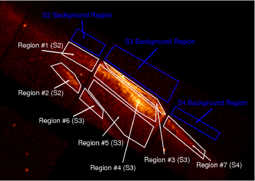
Figure 9: The extraction regions for the spectral analysis of the nonthermal X-ray emission from the northwestern rim complex of G266.2$-$1.2 (see Section 3.2). We have indicated both the seven regions of spectral extraction (in white) as well as the regions where background spectra were extracted (in blue). Also see Table 6.

As described in Section 2, we have extracted spectra from seven regions in the rim complex and in Table 6 we list relevant properties of these regions. With the a priori knowledge that the X-ray emission from the rim complex is predominately non-thermal, we attempted to fit the extracted spectra using three different non-thermal models, described below. To create background spectra for the purposes of our spectral modeling, we extracted spectra from regions located just ahead of the leading edge of the rim complex on each chip. This choice of background helps us to account for diffuse thermal emission seen from the Vela SNR in projection against the rim complex itself (Lu & Aschenbach, 2000; Aschenbach, 2002). In all cases, we have used the photoelectric absorption model PHABS (Arnaud, 1996) to account for the absorption along the line of sight to the northwestern rim complex. The regions considered for spectral analysis (both source regions and the background regions) are depicted in Figure 9. We note that this work extends previous spectral analysis of this rim complex that was presented by Bamba et al. (2005a) by considering the properties of regions sampled by the ACIS-S2, -S3 and -S4 chips instead of just the ACIS-S3 chip.

The first model we considered was a simple power-law. This model has traditionally been used to fit the X-ray spectra extracted from ROSAT and ASCA observations of the X-ray luminous rims of Galactic SNRs that feature non-thermal emission, such as SN 1006 (Koyama et al., 1995) and G347.3$-$0.5 (Slane et al., 1999), as well as G266.2$-$1.2 (Slane et al., 2001a, b). The typical values for the photon indices derived from fits with power-law models to the spectra of these bright rims are $\Gamma$ $\sim$ 2.1–2.6. In the case of G266.2$-$1.2, Slane et al. (2001a) derived a photon index of 2.6$\pm$0.2 when fitting the spectrum of the northwestern rim, and photon indices of $\Gamma$=2.6$\pm$0.2 and $\Gamma$=2.5$\pm$0.2 for fits to the extracted spectra of the northeastern rim and the western rim, respectively. In their spectral analysis of dataset obtained from the XMM-Newton observation of this rim complex, Iyudin et al. (2005) derived a photon index of $\Gamma$ $\sim$ 2.6 for fits to the higher energy emission ($E$ $\geq$ 0.8 keV) emission from the entire complex: this power-law component was combined with thermal components (to model emission separately from the Vela SNR and from G266.2$-$1.2) for modeling the entire broadband emission (0.2 $\leq$ $E$ $\leq$ 10.0 keV). The results of our fits to the spectra of the seven regions in the rim complex using this model are given in Table 7: for each region we give the best fit values for the column density $N$_H, photon index $\Gamma$, the normalizations of each fit and for each ObsID (along with 90% confidence ranges for each of these parameters), the ratio of the values of the $\chi$² to the number of degrees of freedom (i.e., the reduced $\chi$² value) and the absorbed and unabsorbed fluxes. We have performed our fits over the energy range of 1.0 through 5.0 keV for each extracted spectra.

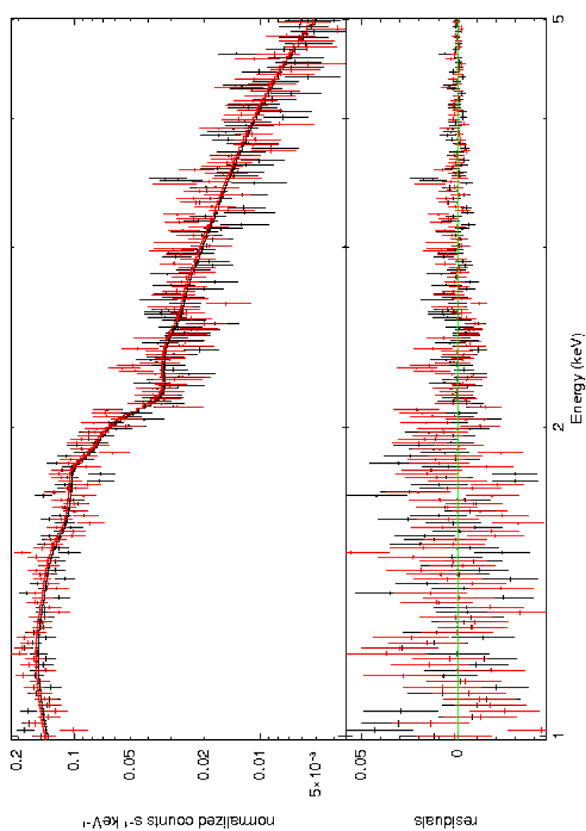
Figure 10: Extracted spectra for Region #3 as fit with a PHABS*Power Law Model (see Table 7). The spectrum from ObsID 3816 is shown in black while the spectrum from ObsID 4414 is shown in red.

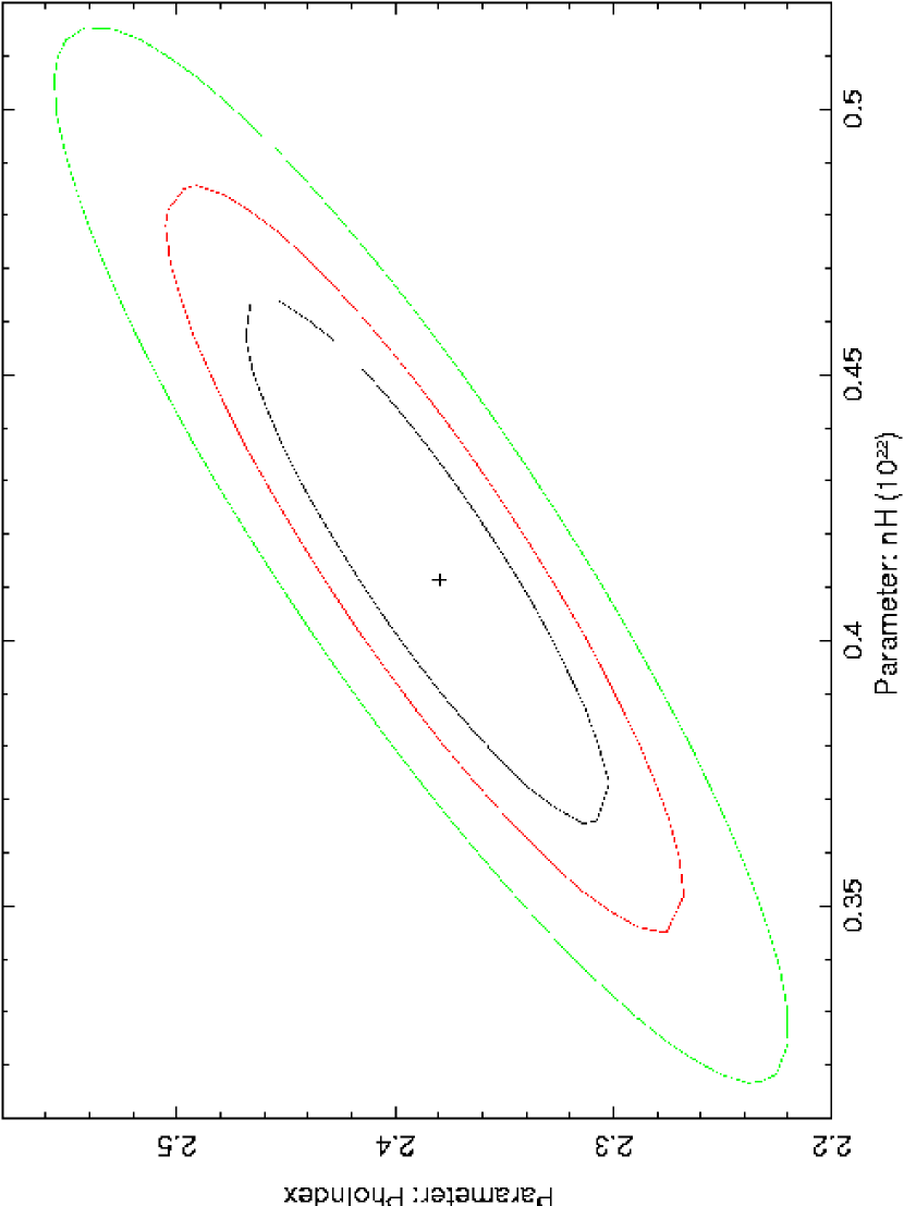
Figure 11: Confidence contours (at the 1$\sigma$, 2$\sigma$ and 3$\sigma$ levels) for the PHABS*Power Law fit to the extracted spectra for Region #3 (see Figure 10 and Table 7).

Statistically acceptable fits have been found for all regions using the power-law model. Our derived photon indices range from approximately 2.38 through 2.70 (in broad agreement with the photon index value measured for the whole complex by Slane et al. (2001a)) and differences are seen in the values of the photon index for different regions. Several regions in the rim complex may actually be physically associated based on similar values for the derived photon indices: one pair of plausibly associated regions are Regions #3 and #7, both of which feature indices of $\Gamma$ $\sim$ 2.38 (the lowest values of photon indices for any of the regions in the rim complex) and appear to form a clearly-defined leading shock. Similarly, Regions #1 and #4 appear to form a feature, seen in projection which trails behind the leading shock (though Region #1 is a leading structure in the portion of the rim complex sampled by the ACIS-S2 chip). Finally, Regions #2 and #6 form a trailing rim that is even more clearly distinct from the leading shock; we suspect that this rim also appears to lie interior to the leading shock simply because of projection effects. In their analysis of XMM-Newton observations of this SNR, Iyudin et al. (2005) first mentioned the presence of this trailing rim though the superior angular resolution of Chandra more clearly resolves this feature as distinct from the leading shock, as noted by Bamba et al. (2005a). We interpret the slight range of values of the photon index to possibly indicate the presence of variations in the shock conditions of accelerated electrons within the complex: the lower index of the leading rim indicates that cosmic-ray electrons are being accelerated to higher energies than at the sites of the regions with higher indices. We will continue to discuss variations in the shock conditions in different portions of the rim complex when we describe our spectral fits with the synchrotron models below. For illustrative purposes, in Figures 10 and 11 we present the extracted spectra of one region (namely Region #3) as fit with the PHABS$\times$Power Law model and confidence contours for this fit, respectively.

The other two models that we used to fit the extracted spectra, SRCUT and SRESC, assume a synchrotron origin for the hard X-ray emission observed from the SNR. Both of these models have been described in detail elsewhere but we provide brief descriptions of each one here. The SRCUT model (Reynolds, 1998; Reynolds & Keohane, 1999; Hendrick & Reynolds, 2001) describes a synchrotron spectrum from an exponentially cut-off power-law distribution of electrons in a uniform magnetic field. This model assumes an electron energy spectrum $N$_e($E$) of the form

$$N_{e}(E)=KE^{-\Gamma}e^{\frac{-E}{E_{\rm{cutoff}}}}$$ (3)

where $K$ is the normalization constant derived from the observed flux density of the region of the SNR at 1 GHz, $\Gamma$ is defined as 2$\alpha$+1 (where $\alpha$ is the radio spectral index) and $E$_cutoff is the maximum energy of the accelerated cosmic-ray electrons. The SRESC model (Reynolds, 1996, 1998) describes a synchrotron spectrum from an electron distribution limited by particle escape above a particular energy. This model describes shock-accelerated electrons in a Sedov blast wave which are interacting with a medium with uniform density and a uniform magnetic field. The SRESC model takes into account variations in electron acceleration efficiency with shock obliquity as well as post-shock radiative and adiabatic losses. Dyer et al. (2001) and Dyer et al. (2004) have described successfully applying the SRESC model to fit extracted X-ray spectra from the bright rims and the interior of SN 1006 using data from observations made by both ASCA and RXTE. A crucial feature of both the SRESC model and the SRCUT model is that a resulting fit made with either of these models can be compared with two observable properties of an SNR, namely its flux density at 1 GHz and radio spectral index $\alpha$. We note that one of the fit parameters of these two models is the cutoff frequency $\nu$_cutoff of the synchrotron spectrum of the accelerated cosmic-ray electrons. This frequency is defined as the frequency at which the flux has dropped from a straight power law by a factor of ten for SRCUT and by a factor of six for SRESC. We can express $\nu$_cutoff as (see, for example, Lazendic et al. (2004))

$$\nu_{\rm{cutoff}}\approx 1.6\times 10^{16}\left(\frac{B_{\rm{\mu G}}}{10~{}\mbox{$\mu$G}}\right)\left(\frac{E_{\rm{cutoff}}}{\mbox{10 TeV}}\right)^{2}\mbox{Hz},$$ (4)

where $B$_μG is the magnetic field strength of the SNR in $\mu$G and it is assumed that the electrons are moving perpendicular to the magnetic field. Based on the value for $\nu$_cutoff returned by the SRESC and SRCUT models as well as its normalization $K$, we can model the synchrotron spectrum of the shock-accelerated cosmic-ray electrons associated with SNRs and estimate the maximum energy $E$_cutoff of the shock-accelerated electrons. We emphasize here that to make this estimate of the cutoff energy, either the magnetic field needs to be measured or a specific value for the magnetic field needs to be assumed.

In applying the SRESC and SRCUT models, the observed radio properties of the SNR – namely the flux density at 1 GHz and $\alpha$ – are needed to constrain the X-ray spectral fits in a meaningful manner. Like many of the other characteristics of G266.2$-$1.2 that were described in Section 1, the radio properties of this SNR have proven to be controversial as well. To investigate the radio properties of this SNR, Combi et al. (1999) used data from the deep continuum survey of the Galactic plane made with the Parkes 64 meter telescope at a frequency of 2.4 GHz and with an angular resolution of 10.4 arcmin as conducted and described by Duncan et al. (1995). Combi et al. (1999) combined this dataset with additional 1.42 GHz data obtained with the 30 meter telescope of the Instituto Argentino de Radioastronomia at Villa Elisa, Argentina: the half-power beamwidth of this instrument at 1.42 GHz is approximately 34 arcminutes. Based on these observations, Combi et al. (1999) claimed to have detected extended limb-brightened features associated with this SNR at the frequencies of 2.4 and 1.42 GHz and argued that the radio morphology of this SNR closely corresponds to the X-ray morphology. Different conclusions were reached by Duncan & Green (2000), however, who performed their own analysis of the 2.4 GHz radio data and also considered data from new radio observations made at 1.40 GHz and 4.85 GHz with the Parkes telescope: the latter data was obtained as part of the Parkes-MIT-NRAO (PMN) survey (Griffith & Wright, 1993) and the angular resolutions of these observations were 14.9 and 5 arcminutes, respectively. Duncan & Green (2000) argued that the extended features described by Combi et al. (1999) are more likely to be associated with the Vela SNR than with G266.2$-$1.2 itself. By considering the radio emission detected within a circle corresponding to the X-ray extent of G266.2$-$1.2, Duncan & Green (2000) measured a spectral index $\alpha$ = 0.40$\pm$0.15 (where $S$_ν $\propto$ $\nu$^-α) for the northern half of the SNR using the method of “T-T” plots as described by Turtle et al. (1962) and argued that this spectral index value was applicable to all of G266.2$-$1.2. They also estimated the integrated fluxes from this SNR at the frequencies of 2.42 and 1.40 GHz to be 33$\pm$6 and 40$\pm$10 Jy, respectively. By extrapolating their measured integrated flux to a frequency of 1 GHz using the above spectral index value, Duncan & Green (2000) estimated the integrated flux from G266.2$-$1.2 at that frequency to be 47$\pm$12 Jy and from this value calculated an average surface brightness of this SNR at 1 GHz to be $\Sigma$_1GHz to be 6.1$\pm$1.5 $\times$ 10^-22 W m^-2 Hz^-1 sr^-1 = 6.1$\pm$1.5 $\times$ 10⁴ Jy sr^-1. The broadband radio observations presented by Stupar et al. (2005) of G266.2$-$1.2 more clearly revealed a shell-like radio morphology for this SNR: in particular, enhanced radio emission at the northwestern rim complex. Using the average surface brightness calculated for this rim complex at 1 GHz (see Section 2.2) and the measured angular sizes of each region, we calculated the corresponding flux density at 1 GHz for that region. The calculated flux densities for each region are provided in Table 6. We then performed our spectral analysis with the SRESC and SRCUT models using these calculated flux densities for the normalizations. These frozen normalizations are necessary to help make meaningful interpretations of fits to the X-ray spectra of these features assuming a synchrotron origin to the emission. Certainly, local variations are expected in the corresponding flux density at 1 GHz for each region: newer radio observations made with higher angular resolution are required to clearly identify such variations and measure the corresponding flux densities.

In Tables 8 and 9 we present the results of our fits to the extracted spectra using the SRCUT and the SRESC model. For each fit we have listed the fit parameters including column density $N$_H, spectral index $\alpha$, cutoff frequency $\nu$_cutoff (along with 90% confidence intervals for each of these parameters), the normalization value used, the ratio of $\chi$² to the number of degrees of freedom for each fit and the corresponding absorbed and unabsorbed fluxes of each region.

4 Estimates of the Maximum Energies of Cosmic-Ray Electrons Accelerated by G266.2$-$1.2 and Other SNRs

Based on the the fit values for the cutoff frequencies derived from fitting the SRCUT model to the spectra of the seven regions, we have used Equation 4 to calculate the maximum energy $E_{\rm cutoff}$ of cosmic-ray electrons accelerated at each of these regions. Following Reynolds & Keohane (1999) and Hendrick & Reynolds (2001), we have assumed a field strength $B=10\ \mu$G, which is expected to be a lower limit on the actual magnetic field strength. In Table 10 we list our computed estimates for $E_{\rm cutoff}$ for each region and each assumed normalization: our estimates for $E_{\rm cutoff}$ for the different regions range from 30 to 40 TeV with the highest estimated value corresponding to the portion of the leading shock that corresponds to Region #7. The higher observed value for $E_{\rm cutoff}$ for this region may indicate that cosmic-ray acceleration is the most robust at this location and that cosmic-ray electrons are accelerated to their highest energies in the narrow regions along the shock front. Once again we point out that the Chandra observations have revealed a possible range of spatial variations in the acceleration of cosmic-ray electrons along the entire rim complex.

In Tables Non-Thermal X-ray Emission from the Northwestern Rim of the Galactic Supernova Remnant G266.2$-$1.2 (RX J0852.0$-$4622) and 12 we present listings of published estimates for the cutoff frequencies of cosmic-ray electrons accelerated by a sample of SNRs in the Galaxy and the Large Magellanic Cloud (LMC), respectively: in each case these estimates have been derived using the SRCUT model. Most of these estimates have been taken from Reynolds & Keohane (1999) and Hendrick & Reynolds (2001) (Tables Non-Thermal X-ray Emission from the Northwestern Rim of the Galactic Supernova Remnant G266.2$-$1.2 (RX J0852.0$-$4622) and 12, respectively). We have included in this list several SNRs (like Kes 73, 3C 396, G11.2$-$0.3 and RCW 103) considered by Reynolds & Keohane (1999) which are now known to be associated with central X-ray sources which contribute confusing hard emission that was not spatially resolved from the SNR itself by the ASCA observations. Therefore, these estimates for $E_{\rm cutoff}$ must be interpreted with caution. In addition, we have augmented the lists from those two papers with published estimates from other papers which have considered other SNRs. Using Equation 4 and again assuming a magnetic field $B=10\ \mu$G, we have calculated a value for $E_{\rm cutoff}$ for each SNR. Lastly, we have added to Table Non-Thermal X-ray Emission from the Northwestern Rim of the Galactic Supernova Remnant G266.2$-$1.2 (RX J0852.0$-$4622) our own estimate for $\nu_{\rm cutoff}$ and $E_{\rm cutoff}$ for G266.2$-$1.2 as described in this paper to help generate an up-to-date listing of values for $E_{\rm cutoff}$ for SNRs both in the Galaxy and in the LMC.

All of the estimates presented here for values of $E_{\rm cutoff}$ must be interpreted with a great deal of caution, given known significant uncertainties in our understanding about the true shape of the electron spectrum and about the magnetic field strength. As shown in Equation 3, the model SRCUT is based on the assumption that the electron spectrum is a power law with an exponential cut off. If the cosmic-ray energy density at the forward shock is large enough, then the shock transition region will be broadened (Ellison & Reynolds, 1991; Berezhko & Ellison, 1998). As a result, cosmic-ray spectra do not have power-law distributions: instead, the spectra flatten with increasing energy (Bell, 1987; Ellison & Reynolds, 1991; Berezhko & Ellison, 1998). Evidence of such curvature has been reported for Cas A (Jones et al., 2003), RCW 86 (Vink et al., 2006) and SN 1006 (Allen et al., 2008b). If magnetic fields in remnants are $\sim 100\ \mu$G or larger, as has been reported for several young remnants, then the electron spectrum should be steepened due to radiative losses (e.g., Ksenofontov et al. (2010)). Furthermore, theoretical analyses presented by other authors (Ellison et al., 2001; Uchiyama et al., 2003; Lazendic et al., 2004; Zirakashvili & Aharonian, 2007) have used an alternative form for the cutoff (that is, $\exp(-(E/E_{\rm cutoff}))^{s}$) where the range of values for $s$ have included 1/4, 1/2, 1 or 2 (though Zirakashvili & Aharonian (2007) have argued in favor of the use of $s=2$). Taken altogether, it is clear that the simple spectral form of the accelerated electrons in Equation 3 (as featured in such models as SRCUT and SRESC) is likely to be a significant over-simplification of the true shapes of the spectra. We comment that the data presently available for G266.2$-$1.2 may not be sensitive enough for very rigorous models of the shape of the electron spectrum. Because the synchrotron emissivity function for a monoenergetic collection of electrons is quite broad (Longair, 1994), the shape of the synchrotron spectrum will be a very broadly smeared version of the shape of the electron spectrum at the energy where the electron spectrum is cutoff. The synchrotron spectrum can also be broadened if the electron spectrum or magnetic field strength vary within a spectral extraction region. We also comment that the cutoff frequency is only one of the parameters in the fit that control the shape of the spectrum: our fits also include a photon index and an absorption column density and the values of these shape parameters are correlated. If the electron spectrum is curved and if radiative losses are important at the cutoff energy in the electron spectrum, then the synchrotron model is clearly over-simplified and should include additional shape parameters. If the electron spectrum is curved due to the pressure of cosmic rays or synchrotron losses or if $s<1$, then the estimates for the maximum electron energies in Tables Non-Thermal X-ray Emission from the Northwestern Rim of the Galactic Supernova Remnant G266.2$-$1.2 (RX J0852.0$-$4622) and 12 are overestimates. Furthermore, the assumed magnetic field strength of $10\ \mu$G is clearly an underestimate for some young SNRs, where the magnetic field is known to be closer to $100\ \mu$G: in such a case, the estimates for the maximum energies given here are certainly overestimates and the true maximum energies may be lower still.

Despite these reasons to expect that the true electron cut-off energies are lower than the values listed in Tables Non-Thermal X-ray Emission from the Northwestern Rim of the Galactic Supernova Remnant G266.2$-$1.2 (RX J0852.0$-$4622) and 12, it is still clear from the augmented tables that no known SNR (either Galactic or in the LMC) appears to be accelerating cosmic-ray electrons to the energy of the knee feature of the cosmic-ray spectrum (that is, approximately 3000 TeV), just as pointed out by Reynolds & Keohane (1999) in referencing their Table 11. From the work in the present paper, we have established that G266.2$-$1.2 does not appear to be accelerating cosmic-ray electrons to the knee feature either: we note that the values listed for $\nu_{\rm cutoff}$ in Tables Non-Thermal X-ray Emission from the Northwestern Rim of the Galactic Supernova Remnant G266.2$-$1.2 (RX J0852.0$-$4622) and 12 are derived from integrated spectra for these SNRs, while we have considered for G266.2$-$1.2 the region with the highest value for $\nu_{\rm cutoff}$. Indeed, wide variations in the values for this quantity have been reported for spatially-resolved spectral analyses of SNRs like SN 1006 (Rothenflug et al., 2004; Allen et al., 2008b) and Cas A (Stage et al., 2006). Also, as stated by Reynolds & Keohane (1999), it must be stressed that these maximum values are most likely overestimates given the assumption that most or all of the X-ray flux from an SNR is non-thermal in origin. Ignoring the contribution of thermal emission is clearly incorrect for SNRs which are known to feature emission lines in their X-ray spectra. We note that additional analyses published by other authors have provided lower limits on the maximum energy of cosmic-ray electrons accelerated by SNRs. For example, in analyzing synchrotron emission at infrared wavelengths from Cas A, Rho et al. (2003) concluded that the maximum energy of cosmic-ray electrons accelerated by that SNR was at least 0.2 TeV. Given the significant losses through synchrotron radiation which are expected from cosmic-ray electrons as they are accelerated to high energies, it is not very surprising that no SNR has been observed to be accelerating cosmic-ray electrons to the energy of the knee feature. The fact that no SNR features an $E_{\rm cutoff}$ value that is near the knee energy is not unexpectedrefle given that the knee feature is more clearly associated with cosmic-ray protons and nucleons. Our analyses place no constraints upon the maximum energy of the nuclei.

5 Conclusions

The conclusions of this paper may be summarized as follows:

1) We have conducted an analysis of two X-ray observations made with Chandra of the luminous northwestern rim complex of the Galactic SNR G266.2$-$1.2: the combined effective integration time of the two observations was 73280 seconds. This SNR is a member of the class of Galactic SNRs which feature X-ray spectra dominated by non-thermal emission, which is commonly interpreted to be synchrotron in origin. We have performed an X-ray spatially-resolved spectral analysis of this rim complex to help probe the phenomenon of non-thermal X-ray emission from SNRs and its relationship to cosmic-ray acceleration by these sources. These observations have revealed fine structure in the rim complex, including a sharply defined leading shock and additional filaments. To help constrain the analysis of synchrotron emission from this rim complex, we have also considered radio observations made of G266.2$-$1.2 with ATCA at the frequencies of 1384 MHz and 2496 MHz.

2) We have modeled the length scales of the upstream X-ray emitting structures located along the northwestern rim complex and sampled by the ACIS-S2, -S3 and -S4 chips. We compared these length scales with published length scales for other non-thermal X-ray-emitting structures associated with the rims of five historical Galactic SNRs. The length scales range from 0.02 to 0.08 pc and are comparable to those measured for the older historical SNRs.

3) We have extracted spectra from seven regions that were sampled using the ACIS-S array (namely the ACIS-S2, ACIS-S3 and ACIS-S4 chips) and fit the spectra using several non-thermal models, namely a simple power-law and the synchrotron models SRCUT and SRESC. Statistically acceptable fits have been derived using each model: however, slight variations are seen in derived fit parameters such as the photon index and cutoff frequency. We interpret the variations of these parameters to possibly indicate differences in how cosmic-ray electrons are accelerated along different sites of the rim complex. We argue that the lower photon index and higher cutoff frequencies derived for the two regions that compose the leading shock (our Regions #3 and #7) are indicative of cosmic-ray electrons being accelerated to the highest energies at these locations.

4) We estimate the maximum energy of cosmic-ray electrons accelerated along this rim complex to be approximately 40 TeV. This maximum energy is associated with Region #7, a region that forms a portion of the leading shock of the rim complex. We have also estimated the maximum energies of cosmic-ray electrons accelerated by other Galactic SNRs and LMC SNRs based on published values of cut-off frequencies. As established in prior works, no known SNR appears to be currently accelerating cosmic-ray electrons to the knee energy of the observed cosmic-ray spectrum (though this knee feature is more applicable for cosmic-ray protons and cosmic-ray nucleons). Such a result is not unexpected, given that significant synchrotron losses from accelerated cosmic-ray electrons are predicted to limit the maximum energies of these accelerated particles to energies significantly below the energies associated with the knee feature.

Figure 1: A mosaicked X-ray image of the Galactic supernova remnant (SNR) G266.2$-$1.2 (RX J0852.0-4622) as prepared from all-sky survey images made with the Position Sensitive Proportional Counter (PSPC) aboard the Röntgensatellit (ROSAT). The emission is shown for photon energies from 1.3 keV to 2.4 keV: we have excluded softer energies to help reduce the effects of confusing emission from the Vela SNR. The image has been smoothed with a Gaussian of 1 arcminute and the plotted scale is 0 to 3.2 counts per pixel (each pixel is approximately 1.7 arcminutes $\times$ 1.7 arcminutes in size). A clear shell-like morphology is seen: the approximate placement of the Advanced CCD Imaging Spectrometer (ACIS) chips (namely chips ACIS-S0, -S1, -S2, -S3, -S4 and-I2) for our observation of the northwestern rim are indicated with red squares.

Figure 2: An ACIS image of the northwestern rim complex of G266.2-1.2: the emission is shown for the energy range 1.0 through 5.0 keV. To boost the signal-to-noise, we have combined datasets from both observations to produce a merged image: we have also smoothed the image with a Gaussian of 1.5 arcseconds. Bright filamentary structure, a leading and trailing rim and a bright leading shock are all apparent in this image and are labeled.

Figure 3: An ACIS image of the northwestern rim complex of G266.2$-$1.2 for the same energy range shown in Figure 2 with radio contours (depicting emission observed at 2496 MHz) overlaid. The contour levels range from 0.005 to 0.070 Jy/beam in steps of 0.005 Jy/beam. The resolution of the radio observation is 120$\arcsec$. See Section 2.

Figure 4: An ACIS mage of the northwestern rim complex of G266.2$-$1.2 for the same energy range shown in Figure 2 with radio contours (depicting emission observed at 1384 MHz) overlaid. The contour levels range from 0.005 to 0.105 Jy/beam in steps of 0.005 Jy/beam. The resolution of the radio observation is 120$\arcsec$. See Section 2.

Figure 5: An ACIS image of the northwestern rim of G266.2$-$1.2 for the same energy range shown in Figure 2. The bright filaments along the outer edge of the remnant are evident. The eight rectangles labeled A–H are the eight regions used to measure the widths of the bright X-ray-emitting filaments. The boxes are centered lengthwise on the portion of the rim with the largest surface brightness and are oriented at the angles that minimized the upstream filament widths $l_{1}$. The asterisk marks the location of the optical axis of the telescope. See Section 3.1 and Table 4).

Figure 6: A histogram of the number of events in Region C as a function of the position $x$ along the long axis of this region (top panel). The position angle of this axis is $312\arcdeg$. The best-fit profile (see Equation 1) is also shown in the top panel. The bottom panel shows the difference between the data and the model divided by the 1 $\sigma$ uncertainties in the data.

Figure 7: The best-fit upstream width $l_{1}$ for Region C as a function of the position angle of the long axis of the extraction region for this region. The smooth curve in the top panel is the parabola (see eqn 2) that best fits the data. The lower panel shows the differences between the data and the model divided by the 1 $\sigma$ uncertainties in the data. The circle marks the best-fit position angle of $312^{\circ}\pm 19^{\circ}$.

Figure 8: The correlation between the best-fit upstream filament widths $l_{1}$ and the angular separations of the centers of the extraction regions and the optical axis of the telescope. A correlation is expected since the point-spread function of the telescope increases as a source is moved away from the optical axis.

Table 1: Summary of Prior Chandra Observations of SNRs with X-ray Spectra Dominated by Non-Thermal Emission

SNR	References
SN 1006	Long et al. (2003), Bamba et al. (2003), Cassam-Chenaï et al. (2008), Allen et al. (2008b), Katsuda et al. (2009a)
G1.9$+$0.3	Reynolds et al. (2008), Reynolds et al. (2009)
G28.6$+$0.1	Ueno et al. (2003)
G266.2$-$1.2	Bamba et al. (2005a)
G330.2$+$1.0	Park et al. (2009)
G347.3$-$0.5	Uchiyama et al. (2003); Lazendic et al. (2004); Uchiyama et al. (2007)

Table 2: Summary of Chandra Observations of the Northwestern Rim of G266.2$-$1.2

						Effective
						Exposure
Sequence		R.A.	Decl.	Roll	Observation	Time
Number	ObsID	(J2000.0)	(J2000.0)	(degrees)	Date	(seconds)
500325	3846	08 49 09.40	$-$45 37 42.41	30	5 January 2003	39363
500325	4414	08 49 09.39	$-$45 37 42.35	30	6 January 2003	33917

Note. — Units of Right Ascension are hours, minutes and seconds, and units of Declination are degrees, arcminutes and arcseconds.

Table 3: Widths of Synchrotron-Emitting X-ray Filaments Associated with Galactic SNRs

			Apparent
			Angular	Filament	Filament	Filament Width
	Distance		Radius	Width	Width	as Fraction of
SNR	(kpc)	Reference	(arcmin)	(arcsec)	(pc)	SNR Radius	References
SN 1006	2.2	(1)	15	4–20	0.04–0.20	0.0044–0.022	(2), (3)
Cas A	3.4	(4)	2.55	3-4	0.05	0.02-0.03	(5), (6)
Kepler	4.8	(7)	1.5	2-3	0.05–0.07	0.02–0.03	(8)
Tycho	2.3	(9)	4	5	0.06	0.021	(8), (10)
RCW 86	2.8	(11)	21	20	0.27	0.016	(8)
G330.2$+$1.0	5.0	(12)	5.5	12–16	0.3–0.4	0.036–0.048	(13)
G347.3$-$0.5	6.3	(14)	30	20–40	0.6–1.2	0.011–0.022	(15), (16)
	1.0	(17)	30	20–40	0.1–0.2

References. — (1) Winkler et al. (2003), (2) Long et al. (2003), (3) Bamba et al. (2003) (4) Reed et al. (1995), (5) Gotthelf et al. (2001), (6) Vink & Laming (2003), (7) Reynoso & Goss (1999), (8) Bamba et al. (2005b), (9) Hughes (2000), (10) Hwang et al. (2002), (11) Rosado et al. (1996), (12) McClure-Griffiths et al. (2001), (13) Park et al. (2009), (14) Slane et al. (1999), (15) Uchiyama et al. (2003), (16) Lazendic et al. (2004), (17) Fukui et al. (2003).

Table 4: Widths of X-ray Emitting Features in Northwestern Rim Complex of G266.2$-$1.2

	R.A.	Dec	$l_{1}$	$\theta_{1}$	$\phi$
Region	(J2000.0)	(J2000.0)	(pixel)	(deg)	(arcmin)
A	08 49 19.44	$-45$ 34 51.2	$16.24^{+1.91}_{-4.69}$	$293\pm 14$	3.4
B	08 49 07.37	$-45$ 35 52.0	$7.04^{+1.21}_{-0.75}$	$308\pm 15$	1.9
C	08 49 03.99	$-45$ 36 16.9	$7.60^{+1.06}_{-0.92}$	$312\pm 19$	1.7
D	08 48 57.37	$-45$ 37 15.6	$10.83^{+1.40}_{-1.05}$	$304\pm 9$	2.2
E	08 48 52.70	$-45$ 37 50.9	$10.80^{+0.77}_{-1.29}$	$306\pm 21$	2.9
F	08 48 47.33	$-45$ 38 27.8	$5.88^{+0.53}_{-0.51}$	$301\pm 9$	3.9
G	08 48 42.69	$-45$ 39 02.7	$17.17^{+0.78}_{-1.02}$	$311\pm 14$	4.9
H	08 48 38.77	$-45$ 39 52.3	$21.67^{+1.88}_{-1.65}$	$325\pm 35$	5.8

Note. — Units of Right Ascencion are hours, minutes and seconds, and units of Declination are degrees, arcminutes and arcseconds.

Table 5: Comparison of Measured Widths of Non-Thermal X-ray Filaments Associated with Galactic SNRs

		$l$1	$l$1	$l$2	$l$2
SNR	Filament	($\arcsec$)	(pc)	($\arcsec$)	(pc)	Reference
SN 1006	#1	1.7 (1.3, 2.2)	0.02 (0.01, 0.02)	160 ($>$92)	1.7 ($>$0.98)	(1)
	#2	14 (9.8, 21)	0.15 (0.10, 0.22)	93 (73, 130)	0.99 (0.78, 1.39)
	#3	2.3 (0.78, 4.3)	0.02 (0.01, 0.05)	150 ($>$56)	1.60 ($>$0.60)
	#4	0.12 (–)	0.001 (–)	150 ($>$78)	1.60 ($>$0.83)
	#5	4.5 (2.2, 8.7)	0.05 (0.02, 0.09)	62 (43, 100)	0.66 (0.46, 1.07)
	#6	3.4 (2.4, 5.0)	0.04 (0.03, 0.05)	130 (86, 250)	1.39 (0.92, 2.67)
Cas A	#1	$<$0.93	$<$0.02	1.27 (0.96, 1.81)	0.02 (0.02, 0.03)	(2)
	#2	$<$0.80	$<$0.01	$<$1.59	$<$0.03
Kepler	#1	1.17 (0.87, 1.59)	0.03 (0.02, 0.04)	0.93 ($<$1.41)	0.02 ($<$0.03)	(2)
	#2	1.59 (1.17, 2.89)	0.04 (0.03, 0.05)	3.09 (3.46, 3.87)	0.07 (0.08, 0.09)
Tycho	#1	1.18 (1.01, 1.32)	0.01 (0.01, 0.01)	5.36 (4.47, 6.12)	0.06 (0.05, 0.07)	(2)
	#2	$<$0.80	$<$0.009	1.70 (1.32, 3.15)	0.02 (0.01, 0.04)
	#3	$<$0.80	$<$0.009	2.38 (2.20, 2.54)	0.03 (0.02, 0.03)
	#4	0.86 (0.80, 0.93)	0.01 (0.009, 0.01)	5.53 (5.00, 6.14)	0.06 (0.06, 0.07)
	#5	1.03 (0.90, 1.35)	0.01 (0.01, 0.02)	2.47 (1.93, 3.15)	0.03 (0.02, 0.04)
RCW 86	#1	2.39 (1.48, 3.34)	0.03 (0.02, 0.05)	20.1 (17.3, 23.8)	0.27 (0.23, 0.32)	(2)
	#2	1.56 (0.49, 4.79)	0.02 (0.007, 0.07)	18.2 (11.8, 35.6)	0.25 (0.16, 0.48)
G266.2$-$1.2	1	19.0 (12.1, 31.4)	0.07 (0.04, 0.11)	31.8 (23.7, 47.1)	0.12 (0.09, 0.17)	(3)
	2	3.68 (2.69, 5.75)	0.01 (0.01, 0.02)	65.0 (38.2, 144.6)	0.24 (0.14, 0.53)
	3	$\cdots$	$\cdots$	37.1 (26.5, 60.2)	0.13 (0.10, 0.22)
G266.2$-$1.2	A	16.24 (11.53, 18.15)	0.06 (0.04, 0.07)	$\cdots$	$\cdots$	(4)
	B	7.04 (6.29, 8.25)	0.03 (0.02, 0.03)	$\cdots$	$\cdots$
	C	7.60 (6.68, 8.66)	0.03 (0.02, 0.03)	$\cdots$	$\cdots$
	D	10.83 (9.78, 12.23)	0.04 (0.03, 0.04)	$\cdots$	$\cdots$
	E	10.80 (9.51, 11.57)	0.04 (0.03, 0.04)	$\cdots$	$\cdots$
	F	5.88 (5.37, 6.41)	0.02 (0.02, 0.02)	$\cdots$	$\cdots$
	G	17.17 (16.15, 17.95)	0.06 (0.06, 0.07)	$\cdots$	$\cdots$
	H	21.67 (20.02, 23.55)	0.08 (0.07, 0.09)	$\cdots$	$\cdots$

Note. — The linear scales have been calculated using the distances for SN 1006, Cas A, Kepler, Tycho and RCW 86 listed in Table Non-Thermal X-ray Emission from the Northwestern Rim of the Galactic Supernova Remnant G266.2$-$1.2 (RX J0852.0$-$4622). In the case of G266.2$-$1.2 the linear scales have been calculated using our adopted distance of 750 pc. All quoted errors are 90% confidence values.

References. — (1) Bamba et al. (2003) (for the 2.0-10.0 keV band), (2) Bamba et al. (2005b) (for the 5.0-10.0 keV band), (3) Bamba et al. (2005a) (for the 2.0-10.0 keV band – the linear scales have been computed assuming a distance to G266.2$-$1.2 of 750 pc), (4) This paper (for the 1.3-5.0 keV band).

Table 6: Properties of the Regions With Extracted Spectra

		Approximate	Approximate	Approximate		Flux
		Central	Central	Region		Density
Region	ACIS-S	R.A.	Decl.	Area	Description	at 1 GHz
Number	Chip	(J2000.0)	(J2000.0)	(arcmin2)	of Location	(Jy)
#1	S2	08 49 24	$-$45 34 52	4.95	Leading Rim	0.036
#2	S2	08 49 32	$-$45 36 48	4.39	Trailing Rim	0.032
#3	S3	08 48 53	$-$45 38 05	5.15	Leading Shock	0.037
#4	S3	08 48 57	$-$45 38 31	10.20	Leading Rim	0.074
#5	S3	08 49 02	$-$45 40 34	18.10	Interior Region	0.131
#6	S3	08 49 17	$-$45 39 34	3.21	Trailing Rim	0.023
#7	S4	08 48 24	$-$45 42 57	5.15	Leading Shock	0.037

Note. — Units of Right Ascencion are hours, minutes and seconds, and units of Declination are degrees, arcminutes and arcseconds.

Table 7: Fits to the Extracted Spectra Using the PHABS$\times$POWER LAW Model

	Column	Photon				Absorbed	Unabsorbed	Absorbed	Unabsorbed
	Density	Index	Normalization	Normalization	$\chi$2/Degrees	Flux	Flux	Flux	Flux
Region	$N$H	$\Gamma$	(ObsID 3846)	(ObsID 4414)	of Freedom	(ObsID 3846)	(ObsID 3846)	(ObsID 4414)	(ObsID 4414)
#1	0.43${}^{+0.09}_{-0.13}$	2.68${}^{+0.14}_{-0.22}$	6.58${}^{+1.12}_{-1.38}$	6.48${}^{+1.12}_{-1.38}$	270.20/279=0.97	7.63$\times$10-13	1.04$\times$10-12	7.52$\times$10-13	1.02$\times$10-12
#2	0.35${}^{+0.12}_{-0.10}$	2.56$\pm$0.18	4.94${}^{+1.06}_{-0.86}$	4.94${}^{+1.06}_{-0.94}$	238.15/263=0.91	6.60$\times$10-13	8.40$\times$10-13	6.60$\times$10-13	8.40$\times$10-13
#3	0.41$\pm$0.07	2.38$\pm$0.12	7.36${}^{+1.04}_{-0.96}$	7.58${}^{+1.02}_{-0.98}$	320.67/343=0.93	1.09$\times$10-12	1.42$\times$10-12	1.12$\times$10-12	1.43$\times$10-12
#4	0.41$\pm$0.05	2.52${}^{+0.09}_{-0.07}$	20.20${}^{+2.00}_{-1.60}$	20.00${}^{+2.00}_{-1.60}$	519.06/477=1.09	2.67$\times$10-12	3.51$\times$10-12	2.65$\times$10-12	3.48$\times$10-12
#5	0.36$\pm$0.10	2.60${}^{+0.14}_{-0.22}$	7.99${}^{+1.61}_{-1.24}$	8.12${}^{+1.68}_{-1.37}$	406.38/393=1.03	1.06$\times$10-12	1.36$\times$10-12	1.08$\times$10-12	1.38$\times$10-12
#6	0.39${}^{+0.21}_{-0.13}$	2.70${}^{+0.35}_{-0.22}$	2.25${}^{+0.75}_{-0.45}$	2.15${}^{+0.75}_{-0.39}$	203.13/194=1.05	2.61$\times$10-13	3.47$\times$10-13	2.50$\times$10-13	3.32$\times$10-13
#7	0.30$\pm$0.14	2.38$\pm$0.18	5.41${}^{+1.69}_{-0.91}$	5.22${}^{+1.16}_{-0.97}$	310.23/277=1.12	8.56$\times$10-13	1.04$\times$10-12	8.26$\times$10-13	1.00$\times$10-12

Table 8: Fits to the Extracted Spectra Using the PHABS$\times$SRCUT Model

	Column	Spectral	Cutoff
	Density	Index	Frequency		$\chi$2/Degrees	Absorbed	Unabsorbed
Region	$N$H	$\alpha$	$\nu$cutoff	Normalization	of Freedom	Flux	Flux
#1	0.18${}^{+0.31}_{-0.05}$	0.54${}^{+0.02}_{-0.10}$	1.65${}^{+1.25}_{-1.25}$	0.036	282.55/280=1.01	7.75$\times$10-13	8.70$\times$10-13
#2	0.17${}^{+0.23}_{-0.05}$	0.55${}^{+0.01}_{-0.08}$	1.83${}^{+1.27}_{-1.28}$	0.032	245.52/264=0.93	6.68$\times$10-13	7.46$\times$10-13
#3	0.32${}^{+0.09}_{-0.05}$	0.52${}^{+0.02}_{-0.03}$	1.85$\pm$1.55	0.037	325.13/344=0.95	1.11$\times$10-12	1.34$\times$10-12
#4	0.24${}^{+0.20}_{-0.03}$	0.52${}^{+0.01}_{-0.08}$	1.58$\pm$0.98	0.074	549.07/478=1.15	2.70$\times$10-12	3.13$\times$10-12
#5	0.21${}^{+0.19}_{-0.05}$	0.59${}^{+0.02}_{-0.07}$	1.93${}^{+1.27}_{-1.28}$	0.131	410.81/394=1.04	1.09$\times$10-12	1.24$\times$10-12
#6	0.17${}^{+0.39}_{-0.07}$	0.58${}^{+0.01}_{-0.15}$	1.92$\pm$1.69	0.023	212.45/195=1.09	2.63$\times$10-13	2.93$\times$10-13
#7	0.21${}^{+0.10}_{-0.08}$	0.54${}^{+0.01}_{-0.03}$	2.80$\pm$1.60	0.037	314.72/278=1.13	8.42$\times$10-13	9.64$\times$10-13

Table 9: Fits to the Extracted Spectra Using the PHABS$\times$SRESC Model

	Column	Spectral	Cutoff
	Density	Index	Frequency		$\chi$2/Degrees	Absorbed	Unabsorbed
Region	$N$H	$\alpha$	$\nu$cutoff	Normalization	of Freedom	Flux	Flux
#1	0.39${}^{+0.05}_{-0.22}$	0.50${}^{+0.06}_{-0.02}$	2.47${}^{+5.33}_{-0.47}$	0.036	273.06/280=0.98	7.51$\times$10-13	9.90$\times$10-13
#2	0.37${}^{+0.05}_{-0.25}$	0.51${}^{+0.07}_{-0.02}$	2.59${}^{+8.61}_{-0.59}$	0.032	245.25/264=0.93	6.48$\times$10-13	8.39$\times$10-13
#3	0.51${}^{+0.04}_{-0.36}$	0.49${}^{+0.09}_{-0.01}$	2.63${}^{+24.67}_{-0.23}$	0.037	362.21/344=1.05	1.06$\times$10-12	1.50$\times$10-12
#4	0.41${}^{+0.04}_{-0.20}$	0.48${}^{+0.06}_{-0.01}$	2.86${}^{+6.24}_{-0.28}$	0.074	540.18/478=1.13	2.61$\times$10-12	3.46$\times$10-12
#5	0.38${}^{+0.06}_{-0.26}$	0.56${}^{+0.07}_{-0.02}$	2.79${}^{+10.71}_{-0.69}$	0.131	413.90/394=1.05	1.04$\times$10-12	1.37$\times$10-12
#6	0.39${}^{+0.09}_{-0.25}$	0.52${}^{+0.08}_{-0.03}$	1.88${}^{+6.12}_{-0.60}$	0.023	205.49/195=1.05	2.50$\times$10-13	3.34$\times$10-13
#7	0.42${}^{+0.03}_{-0.40}$	0.50${}^{+0.10}_{-0.01}$	2.47${}^{+31.53}_{-0.07}$	0.037	337.09/278=1.21	8.10$\times$10-13	1.07$\times$10-12

Table 10: Estimates from the SRCUT Model for Cutoff Energies $E$_cutoff of Cosmic-Ray Electrons Accelerated at Different Regions of the Northwestern Rim Complex of G266.2$-$1.2

	Cutoff	Cutoff
	Frequency	Energy
	$\nu$cutoff	$E$cutoff
Region	(1017 Hz)	(TeV)
#1	1.65${}^{+1.25}_{-1.25}$	30
#2	1.83${}^{+1.27}_{-1.28}$	30
#3	1.85$\pm$1.55	30
#4	1.58$\pm$0.98	30
#5	1.93${}^{+1.27}_{-1.28}$	30
#6	1.92$\pm$1.69	30
#7	2.80$\pm$1.60	40

Table 11: Cutoff Frequencies and Cutoff Energies of Cosmic-Ray Electrons Accelerated by Galactic SNRs As Derived from the SRCUT Model

	Cutoff	Cutoff
	Frequency	Energy
	$\nu$cutoff	$E$cutoff
SNR	(Hz)	(TeV)	References
CTB 37B	3.6$\times$1018	150	(1)
Kes 73	1.5$\times$1018	100	(2)
G1.9$+$0.3	1.4$\times$1018	90	(3)
Cas A	9.0$\times$1017	80	(4)
	3.2$\times$1017	50	(2)
G28.6$-$0.1	7.0$\times$1017	70	(4)
G330.2$+$1.0	3.3$\times$1017	50	(6)
G266.2$-$1.2	2.8$\times$1017	40	(7)
G156.2$+$5.7	2.4$\times$1017	40	(8)
	1.5$\times$1016	9.7	(9)
G347.3$-$0.5	6.3$\times$1017	60	(10)
	2.3$\times$1017	40	(11)
	2.2$\times$1017	40	(12)
SN 1006	1.1$\times$1017	30	(13)
	6.0$\times$1016	20	(14)
Kepler	1.1$\times$1017	30	(2)
Tycho	8.8$\times$1016	20	(2)
RCW 86	8.5$\times$1016	20	(15)
G352.7$-$0.1	6.6$\times$1016	20	(2)
3C 397	3.4$\times$1016	20	(2)
W49B	2.4$\times$1016	10	(2)
G349.7$+$0.2	1.8$\times$1016	10	(2)
3C 396	1.6$\times$1016	10	(2)
G346.6$-$0.2	1.5$\times$1016	9.7	(2)
3C 391	1.4$\times$1016	9.4	(2)
G11.2$-$0.3 (SN 386)	1.2$\times$1016	8.7	(2)
RCW 103	1.2$\times$1016	8.7	(2)

References. — (1) Nakamura et al. (2009), (2) Reynolds & Keohane (1999), (3) Reynolds et al. (2008), (4) Stage et al. (2006), (5) Ueno et al. (2003), (6) Park et al. (2009), (7) This paper, (8) Pannuti & Allen (2004), (9) Katsuda et al. (2009b), (10) Lazendic et al. (2004), (11) Takahashi et al. (2008), (12) Pannuti et al. (2003), (13) Allen et al. (2008b), (14) Reynolds (1996), (15) Rho et al. (2002).

Table 12: Cutoff Frequencies and Cutoff Energies of Cosmic-Ray Electrons Accelerated by Large Magellanic Cloud SNRs As Derived From the SRCUT Model

	Cutoff	Cutoff
	Frequency	Energy
	$\nu$cutoff	$E$cutoff
SNR	(Hz)	(TeV)
DEM L71	2.49$\times$1017	40
N49B	6.76$\times$1016	20
N103B	4.35$\times$1016	20
N23	4.11$\times$1016	20
N132D	3.14$\times$1016	10
0509$-$67.5	2.90$\times$1016	10
0548$-$70.4	1.93$\times$1016	10
N63A	1.93$\times$1016	10
0534$-$69.9	2.42$\times$1015	3.9
0519$-$69.0	1.45$\times$1015	3.0
0453$-$68.5	9.66$\times$1014	2.5

References

- Acero et al. (2010) Acero, F., Aharonian, F. A., Akhperjanian, A. G., Anton, G., Barres de Almeida, U., Bazer-Bachi, A. R., Becherini, Y., Behera, B., Beilicke, M., Bernlöhr, K., Bochow, A., Boisson, C., et al. 2010, A&A, 516, 62
- Aharonian et al. (2004) Aharonian, F. A., Akhperjanian, A. G., Aye, K.-M., Bazer-Bachi, A. R., Beilicke, M., Benbow, W., Berge, D., Berghaus, P., Bernlöhr, K., Bolz, O., Boisson, C., Borgmeier, C., et al. 2004, Nature, 432, 75
- Aharonian et al. (2005) Aharonian, F. A., Akhperjanian, A. G., Bazer-Bachi, A. R., Beilicke, M., Benbow, W., Berge, D., Bernlöhr, K., Boisson, C., Bolz, O., Borrel, V., Braun, I., Breitling, F., et al. 2005, A&A, 437, L7
- Aharonian et al. (2006) Aharonian, F. A., Akhperjanian, A. G., Bazer-Bachi, A. R., Beilicke, M., Benbow, W., Berge, D., Bernlöhr, K., Boisson, C., Bolz, O., Borrel, V., Braun, I., Breitling, F., et al. 2006, A&A, 449, 223
- Aharonian et al. (2007a) Aharonian, F. A., Akhperjanian, A. G., Bazer-Bachi, A. R., Beilicke, M., Benbow, W., Berge, D., Bernlöhr, K., Boisson, C., Bolz, O, Borrel, V., Braun, I., Brown, A. M., et al., 2007a, ApJ, 661, 236
- Aharonian et al. (2007b) Aharonian, F. A., Akhperjanian, A. G., Bazer-Bachi, A. R., Beilicke, M., Benbow, W., Berge, D., Bernlöhr, K, Boisson, C., Bolz, O., Borrel, V., Braun, I., Brion, E., et al. 2007b, A&A, 464, 235
- Allen et al. (1997) Allen, G. E., Keohane, J. W., Gotthelf, E. V., Petre, R., Jahoda, K., Rothschild, R. E., Lingenfelter, R. E., Heindl, W. A., Marsden, D., Gruber, D. E., Pelling, M. R. & Blanco, P. R. 1997, ApJ, 487, L97
- Allen et al. (2001) Allen, G. E., Petre, R. & Gotthelf, E. V. 2001, ApJ, 558, 739
- Allen et al. (2008a) Allen, G. E., Stage, M. D., & Houck, J. C. 2008a, International Cosmic Ray Conference, 2, 839
- Allen et al. (2008b) Allen, G. E., Houck, J. C. & Sturner, S. J. 2008b, ApJ, 683, 773
- Aschenbach et al. (1995) Aschenbach, B., Egger, R. & Trümper, J. 1995, Nature, 373, 587
- Arnaud (1996) Arnaud, K. A. 1996, Astronomical Data Analysis Software and Systems V, eds. Jacoby, G. and Barnes, J., p17, ASP Conf. Series Volume 101.
- Aschenbach (1998) Aschenbach, B. 1998, Nature, 396, 141
- Aschenbach et al. (1999) Aschenbach, B., Iyudin, A. F. & Schönfelder, V. 1999, A&A, 350, 997
- Aschenbach (2002) Aschenbach, B. 2002, Proceedings of the 270th WE-Heraeus Seminar on Neutron Stars, Pulsars and Supernova Remnants, Physikzentrum Bad Honnef, eds. W. Becker, H. Lesch & J. Trümper, MPE Report 278, 18 (astro-ph/0208492)
- Bamba et al. (2001) Bamba, A., Ueno, M., Koyama, K. & Yamauchi, S. 2001, PASJ, 53, L21
- Bamba et al. (2003) Bamba, A., Yamazaki, R., Ueno, M. & Koyama, K. 2003, ApJ, 589, 827
- Bamba (2004) Bamba, A. 2004, Ph.D Thesis, Kyoto University
- Bamba et al. (2005a) Bamba, A., Yamazaki, R. & Hiraga, J. S. 2005a, ApJ, 632, 294
- Bamba et al. (2005b) Bamba, A., Yamazaki, R., Yoshida, T., Terasawa, T. & Koyama, K. 2005b, ApJ, 621, 793
- Bamba et al. (2008) Bamba, A., Fukazawa, Y., Hiraga, J. S., Hughes, J. P., Katagiri, H., Kokubun, M., Koyama, K., Miyata, E., Mizuno, T., Mori, K., Nakajima, H., Ozaki, M., et al. 2008, PASJ, 60, 153
- Bell (1987) Bell, A. R. 1987, MNRAS, 225, 615
- Benbow (2005) Benbow, W., for the HESS Collaboration, in proceedings of the Gamma 2004 Symposium on High-Energy Gamma-Ray Astronomy, Vol. 745 (AIP Conference Proceedings, eds. F.A. Aharonian, H. J. V”olk and D. Horns), 611
- Berezhko & Ellison (1998) Berezhko, E. G. & Ellison, D. C. 1999, ApJ, 526, 389
- Berezhko & Völk (2008) Berezhko, E. G. & Völk, H. J. 2008, A&A, 492, 695
- Borkowski et al. (2001) Borkowski, K. J., Rho, J., Reynolds, S. P. & Dyer, K. K. 2001, ApJ, 550, 334
- Burgess & Zuber (2000) Burgess, C. P. & Zuber, K. 2000, Astroparticle Physics, 14, 1
- Cassam-Chenaï et al. (2004) Cassam-Chenaï, G., Decourchelle, A., Ballet, J., Sauvageot, J.-L., Dubner, G. & Giacani, E. 2004, A&A, 427, 199
- Cassam-Chenaï et al. (2008) Cassam-Chenaï, G., Hughes, J. P., Reynoso, E. M., Badenes, C. & Moffett, D. 2008, ApJ, 680, 1180
- Cha et al. (1999) Cha, A. N., Sembach, K. R. & Danks, A. C. 1999, ApJ, 515, L25
- Chen & Gehrels (1999) Chen, W. & Gehrels, N. 1999, ApJ, 514, L103
- Combi et al. (1999) Combi, J. A., Romero, G. E. & Benaglia, P. 1999, ApJ, 519, L177
- Duncan et al. (1995) Duncan, A. R., Stewart, R. T., Haynes, R. F. & Jones, K. L. 1995, MNRAS, 277, 36
- Duncan & Green (2000) Duncan, A. R. & Green, D. A., 2000, A&A, 364, 732
- Dyer et al. (2001) Dyer, K. K., Reynolds, S. P., Borkowski, K. J., Allen, G. E. & Petre, R. 2001, ApJ, 551, 439
- Dyer et al. (2004) Dyer, K. K., Reynolds, S. P. & Borkowski, K. J. 2004, ApJ, 600, 752
- Ellison & Reynolds (1991) Ellison, D. C. & Reynolds, S. P. 1991, ApJ, 382, 242
- Ellison et al. (2001) Ellison, D. C., Slane, P. O. & Gaensler, B. M. 2001, ApJ, 563, 191
- Ellison & Vladimirov (2008) Ellison, D. C. & Vladimirov, A. 2008, ApJ, 673, L47
- Enomoto et al. (2002) Enomoto, R., Tanimori, T., Naito, T., Yoshida, T., Yanagita, S., Mori, M., Edwards, P. G., Asahara, A., Bicknell, G. V., Gunji, S., Hara, S., Hara, T. et al., 2002, Nature, 416, 823
- Fang et al. (2009) Fang, J., Zhang, L., Zhang, J. F., Tang, Y.Y. & Yu, H. 2009, MNRAS, 392, 925
- Filipović et al. (2001) Filipović, M. D., Jones, P. A. & Aschenbach, B. 2001, “Young Supernova Remnants: Eleventh Astrophysics Conference,” AIP Conference Proceedings, Volume 565, pp. 267
- Fruscione et al. (2006) Fruscione, A. et al. 2006, Proc. SPIE, 6270, 60
- Fukui et al. (2003) Fukui, Y., Moriguchi, Y., Tamira, K., Yamamoto, H., Tawara, Y., Mizuno, N., Onishi, T., Mizuno, A., Uchiyama, Y., Hiraga, J., Takahashi, T., Yamashita, K. & Ikeuchi, S. 2003, PASJ, 55, L61
- Garmire et al. (2003) Garmire, G. P., Bautz, M. W., Ford, P. G., Nousek. J. A. & Ricker, Jr., G. R. 2003, SPIE, 4851, 28
- Gooch (2006) Gooch, R., 2006, KARMA Users Manual, ATNF
- Gotthelf et al. (2001) Gotthelf, E. V., Koralesky, B., Rudnick, L., Jones, T. W., Hwang, U. & Petre, R. 2001, ApJ, 552, L39
- Green & Stephenson (2004) Green, D. A. & Stephenson, F. R. 2004, Astroparticle Physics, 20, 613
- Green (2009a) Green, D. A., 2009a, Bulletin of the Astronomical Society of India, 37, 45.
- Green (2009b) Green, D. A., 2009b, ‘A Catalogue of Galactic Supernova Remnants (2009 March version)’, Astrophysics Group, Cavendish Laboratory, Cambridge, United Kingdom (available at “http://www.mrao.cam.ac.uk/surveys/snrs/”).
- Griffith & Wright (1993) Griffith, M. R. & Wright, A. E. 1993, AJ, 105, 1666
- Hara et al. (1993) Hara, T. et al. 1993, Nucl. Instr. Meth. Phys. Res. A 332, 300
- Helder & Vink (2008) Helder, E. A. & Vink, J. 2008, ApJ, 686, 1094
- Hendrick & Reynolds (2001) Hendrick, S. P. & Reynolds, S. P. 2001, ApJ, 559, 903
- Hiraga et al. (2005) Hiraga, J. S., Uchiyama, Y., Takahashi, T. & Aharonian, F. A. 2005, A&A, 431, 953
- Hiraga et al. (2009) Hiraga, J. S., Kobayashi, Y., Tamagawa, T., Hayato, A., Bamba, A., Terada, Y., Petre, R., Katagiri, H. & Tsunemi, H. 2009, PASJ, 61, 275
- Holt et al. (1994) Holt, S. S., Gotthelf, E. V., Tsunemi, H. & Negoro, H. 1994, PASJ, 46, L151
- Huang et al. (2007) Huang, C.-Y., Park, S.-E., Pohl, M. & Daniels, C. D. 2007, Astroparticle Physics, 27, 429
- Hughes (2000) Hughes, J. P. 2000, ApJ, 545, L53
- Hwang et al. (2000) Hwang, U., Holt, S. S. & Petre, R. 2000, ApJ, 537, L118
- Hwang et al. (2002) Hwang, U., Decourchelle, A., Holt, S. S. & Petre, R. 2002, ApJ, 581, 1101
- Iyudin et al. (1998) Iyudin, A. F., Schönfelder, V., Bennett, K., Bloemen, H., Diehl, R., Hermsen, W., Lichti, G. G., van der Meulen, R. D., Ryan, J. & Winkler, C. 1998, Nature, 396, 142
- Iyudin et al. (2005) Iyudin, A. F., Aschenbach, B., Becker, W., Dennerl, K. & Haberl, F. 2005, A&A, 429, 225
- Jones et al. (2003) Jones, T. J., Rudnick, L., DeLaney, T. & Bowden, J. 2003, ApJ, 587,227
- Katagiri et al. (2005) Katagiri, H., Enomoto, R., Ksenofontov, L. T., Mori, M., Adachi, Y., Asahara, A., Bicknell, G. V., Clay, R. W., Doi, Y., Edwards, P. G., Gunji, S., Hara, S. et al. 2005, ApJ, 619, L163
- Katsuda et al. (2008) Katsuda, S., Tsunemi, H. & Mori, K., 2008, ApJ, 678, L35
- Katsuda et al. (2009a) Katsuda, S., Petre, R., Long, K. S., Reynolds, S. P., Winkler, P. F., Mori, K. & Tsunemi, H. 2009a, ApJ, 692, L105
- Katsuda et al. (2009b) Katsuda, S., Petre, R., Hwang, U., Yamaguchi, H., Mori, K. and Tsunemi, H. 2009b, PASJ, 61, S155
- Katz & Waxman (2008) Katz, B. & Waxman, E. 2008, J. Cosmology Astropart. Phys, 1, 18
- Kawachi et al. (2001) Kawachi, A., Hayami, Y., Jimbo, J., Kamei, S., Kifune, T., Kubo, H., Kushida, J., LeBohec, S., Miyawaki, K., Mori, M., Nishijima, K., Patterson, J. R., et al. 2001, Astroparticle Physics, 14, 261
- Keohane (1998) Keohane, J. W. 1998, Ph.D Thesis, University of Minnesota
- Ksenofontov et al. (2010) Ksenofontov, L. T., Völk, H. J., Berezhko, E. G. 2010, ApJ, 714, 1187
- Koyama et al. (1995) Koyama, K., Petre, R., Gotthelf, E. V., Hwang, U., Matsuura, M., Ozaki, M. & Holt, S. S. 1995, Nature, 378, 255
- Koyama et al. (1997) Koyama, K., Kinugasa, K., Matsuzaki, K., Nishiuchi, M., Sugizaki, M., Torii, K., Yamauchi, S. & Aschenbach, B. 1997, PASJ, 49, L7
- Koyama et al. (2001) Koyama, K., Ueno, M., Bamba, A. & Ebisawa, K. 2001, Proceedings of the Symposium “New Visions of the X-ray Universe in the XMM-Newton and Chandra Era,” Noordwijk, The Netherlands (arXiv: astro-ph/0202009)
- Lazendic et al. (2004) Lazendic, J. S., Slane, P. O., Gaensler, B. M., Reynolds, S. P., Plucinsky, P. P. and Hughes, J. P. 2004, ApJ, 602, 271
- Long et al. (2003) Long, K. S., Reynolds, S. P., Raymond, J. C., Winkler, P. F., Dyer, K. K. & Petre, R. 2003, ApJ, 586, 1162
- Longair (1994) Longair, M. S. (1994), High Energy Astrophysics, Volume 2, Stars, the Galaxy and the Interstellar Medium, Cambridge University Press, Cambridge, UK.
- Lu & Aschenbach (2000) Lu, F. J. & Aschenbach, B. 2000, A&A, 362, 1083
- Lyutikov & Pohl (2004) Lyutikov, M. & Pohl, M. 2004, ApJ, 609. 785
- Maeda et al. (2009) Maeda, Y., Uchiyama, Y., Bamba, A., Kosugi, H., Tsunemi, H., Helder, E. A., Vink, J., Kodaka, N., Terada, Y., Fukazawa, Y., Hiraga, J., Hughes, J. P., Kokubun, M., Kouzu, T., Matsumoto, H., Miyata, E., Nakamura, R., Okada, S., Someya, K., Tamagawa, T., Tamura, K., Totsuka, K., Tsuboi, Y., Ezoe, Y., Holt, S. S., Ishida, M., Kamae, T., Petre, R. & Takahashi, T. 2008, PASJ, 61, 1217
- Malkov et al. (2005) Malkov, M. A., Diamond, P. H. & Sagdeev, R. Z. 2005, ApJ, 624, L37
- May et al. (1988) May, J., Murphy, D. C. & Thaddeus, P. 1988, A&AS, 73, 51
- McClure-Griffiths et al. (2001) McClure-Griffiths, N. M., Green, A. J., Dickey, J. M., Gaensler, B. M., Haynes, R. F. & Wieringa, M. H. 2001, ApJ, 551, 394
- Mereghetti (2001) Mereghetti, S. 2001, ApJ, 548, L213
- Moraitis & Mastichiadis (2007) Moraitis, K. & Mastichiadis, A. 2007, A&A, 462, 173
- Morlino et al. (2009) Morlino, G., Amato, E. & Blasi, P. 2009, MNRAS, 392, 240
- Motizuki et al. (2009) Motizuki, Y., Takahashi, K., Makishima, K., Bamba, A., Nakai, Y., Yano, Y., Igarashi, M., Motoyama, H., Kamiyama, K., Suzuki, K. & Imamura, T. 2009, Nature, submitted (http://arxiv.org/abs/0902.3446)
- Muraishi et al. (2000) Muraishi, H., Tanimori, T., Yanagita, S., Yoshida, T., Moriya, M., Kifune, T., Dazeley, S. A., Edwards, P. G., Gunji, S., Hara, S., Hara, T., Kawachi, A., et al. 2000, A&A, 354, L57
- Murphy (1985) Murphy, D. C. 1985, Ph.D Thesis, Massachusetts Institute of Technology
- Nakamura et al. (2009) Nakamura, R., Bamba, A., Ishida, M., Nakajima, H., Yamazaki, R., Terada, Y., Pühlhofer, G. & Wagner, S. J. 2009, PASJ, 61, 197
- Ogasawara et al. (2007) Ogasawara, T., Yoshida, T., Yamagita, S. & Kifune, T. 2007, Ap&SS, 309, 401
- Pannuti et al. (2003) Pannuti, T. G., Allen, G. E., Houck, J. C. & Sturner, S. J. 2003, ApJ, 593, 377
- Pannuti & Allen (2004) Pannuti, T. G. & Allen, G. E. 2004, AdSpR, 33, 434
- Park et al. (2009) Park, S., Kargaltsev, O., Pavlov, G. G., Mori, K., Slane, P. O., Hughes, J. P., Burrows, D. N. and Garmire, G. P. 2009, ApJ, 695, 431
- Pavlov et al. (2001) Pavlov, G. G., Sanwal, D., Kiziltan, B. & Garmire, G. P. 2001, ApJ, 559, L131
- Pellizzoni et al. (2002) Pellizzoni, A., Mereghetti, S. & De Luca, A. 2002, A&A, 393, L65
- Plaga (2008) Plaga, R. 2008, New Astronomy, 13, 73
- Pohl et al. (2005) Pohl, M., Yan, H. & Lazarian, A. 2005, ApJ, 626, L101
- Redman et al. (2000) Redman, M. P., Meaburn, J., O’Connor, J. A., Holloway, A. J. & Bryce, M. 2000, ApJ, 543, L153
- Redman et al. (2002) Redman, M. P., Meaburn, J., Bryce, M., Harman, D. J. & O’Brien, T. J. 2002, MNRAS, 336, 1093
- Redman & Meaburn (2005) Redman, M. P. & Meaburn, J. 2005,MNRAS, 356, 969
- Reed et al. (1995) Reed, J. E., Hester, J. J., Fabian, A. C. and Winkler, P. F. 1995, ApJ, 440, 706
- Reimer & Pohl (2002) Reimer, O. & Pohl, M. 2002, A&A, 390, L43
- Reynolds (1996) Reynolds, S. P. 1996, ApJ, 459, L13
- Reynolds (1998) Reynolds, S. P. 1998, ApJ, 493, 375
- Reynolds & Keohane (1999) Reynolds, S. P. & Keohane, J. W. 1999, ApJ, 525, 368
- Reynolds et al. (2007) Reynolds, S. P., Borkowski, K. J., Hwang, U., Hughes, J. P., Badenes, C., Laming, J. M. & Blondin, J. M. 2007, ApJ, 668, L135
- Reynolds et al. (2008) Reynolds, S. P., Borkowski, K. J., Green, D. A., Hwang, U., Harrus, I. & Petre, R. 2008, ApJ, 680, L41
- Reynolds et al. (2009) Reynolds, S. P., Borkowski, K. J., Green, D. A., Hwang, U., Harrus, I. & Petre, R. 2009, ApJ, 695, L149
- Reynoso & Goss (1999) Reynoso, E. M. & Goss, W. M. 1999, AJ, 118, 926
- Rosado et al. (1996) Rosado, M., Ambrocio-Cruz, P., Le Coarer, E. & Marcelin, M. 1996, A&A, 315, 243
- Rho et al. (2002) Rho, J., Dyer, K. K., Borkowski, K. J. & Reynolds, S.P. 2002, ApJ, 581, 1116
- Rho et al. (2003) Rho, J., Reynolds, S. P., Reach, W. T., Jarrett, T. H., Allen, G. E. & Wilson, J. C. 2003, ApJ, 592, 299
- Rood et al. (1979) Rood, R. T., Sarazin, C. L., Zeller, E. J. & Parker, B. C. 1979, Nature, 282, 701
- Rothenflug et al. (2004) Rothenflug, R., Ballet., J., Dubner, G., Giacani, E., Decourchelle, A. & Ferrando, P. 2004, A&A, 425, 121
- Sankrit et al. (2003) Sankrit, R., Blair, W. P. & Raymond, J. C. 2003, ApJ, 589, 242
- Sault & Killeen (2006) Sault, R. & Killeen, N. 2006, MIRIAD Users Guide, ATNF
- Schönfelder et al. (2000) Schönfelder, V., Bloemen, H., Collmar, W., Diehl, R., Hermsen, W., Knödlseder, J., Lichti, G. G., Plüschke, S., Ryan, J., Strong, A. & Winkler, C. 2000, in AIP Conf. Proc. 510, Fifth Compton Symposium, ed. M. L. McConnell & J. M. Ryan (New York: AIP), 54
- Slane et al. (1999) Slane, P., Gaensler, B. M., Dame, T. M., Hughes, J. P., Plucinsky, P. P. & Green, A. 1999, ApJ, 525, 357
- Slane et al. (2001a) Slane, P., Hughes, J. P., Edgar, R. J., Plucinsky, P. P., Miyata, E., Tsunemi, H. & Aschenbach, B. 2001a, ApJ, 548, 814
- Slane et al. (2001b) Slane, P., Hughes, J. P., Edgar, R. J., Plucinsky, P. P., Miyata, E., Tsunemi, H. & Aschenbach, B. 2001b, in Holt, S. S. Hwang, U., eds, Young Supernova Remnants, AIP, New York, p. 403
- Stage et al. (2006) Stage, M. D., Allen, G. E., Houck, J. C. & Davis, J. E. 2006, NatPh, 2, 614
- Stupar et al. (2005) Stupar, M., Filipović, M. D., Jones, P. A. & Parker, Q. A. 2005, AdSpR, 35, 1047
- Sugizaki (1999) Sugizaki, M. 1999, Ph.D Thesis, University of Tokyo
- Takahashi et al. (2008) Takahashi, T., Tanaka, T., Uchiyama, Y., Hiraga, J. S., Nakazawa, K., Watanabe, S., Bamba, A., Hughes, J. P., Katagiri, H., Takaoka, J., Kokubun, M., Koyama, K., Mori, K., Petre, R., Takahashi, H. & Tsuboi, Y. 2008, PASJ, 60, 131
- Tanaka et al. (2008) Tanaka, T., Uchiyama, Y., Aharonian, F. A., Takahashi, T., Bamba, A., Hiraga, J. S., Kataoka, J., Kishishita, T., Kokubun, M., Mori, K., Nakazawa, K., Petre, R. et al. 2008, ApJ, 685, 988
- Tanimori et al. (1998) Tanimori, T., Hayami, Y., Kamei, S., Dazeley, S. A., Edwards, P. G., Gunji, S., Hara, S., Hara, T., Holder, J., Kawachi, A., Kifune, T., Kita, R., et al. 1998, ApJ, 497, L25
- Telezhinsky (2009) Telezhinsky, I. 2009, APh, 31, 431
- Torii et al. (2006) Torii, K., Uchida, H., Hasuike, K., Tsunemi, H., Yamauchi, Y. & Shibata, S., PASJ, 58, L11
- Tsunemi et al. (2000) Tsunemi, H., Miyata, E., Aschenbach, B., Hiraga, J. & Akutsu, D. 2000, PASJ, 52, 887
- Turtle et al. (1962) Turtle, A. J., Pugh, J. F., Kenderdine, S., Pauliny-Toth, I. I. K. 1962, MNRAS, 124, 297
- Uchiyama et al. (2003) Uchiyama, Y., Aharonian, F. A. & Takahashi, T. 2003, A&A, 400, 567
- Uchiyama et al. (2007) Uchiyama, Y., Aharonian, F. A., Tanaka, T., Takahashi, T. & Maeda, Y. 2007, Nature, 449, 576
- Ueno et al. (2003) Ueno, M., Bamba, A., Koyama, K. & Ebisawa, K. 2003, ApJ, 588, 338
- van der Swaluw & Achterberg (2004) van der Swaluw, E. & Achterberg, A. 2004, A&A, 421, 1021
- Vink (2004) Vink, J. 2003, “The Restless High Energy Universe” Conference Proceedings, Nucl. Physics B. Suppl. Series, eds. E. P. J. van den Heuvel, J. J. M. in ’t Zand & R. A. M. J. Wijers, 132, 21
- Vink et al. (2003) Vink, J., Laming, J. M., Gu, M. F., Rasmussen, A. & Kaastra, J. S. 2003, ApJ, 587, L31
- Vink & Laming (2003) Vink, J. & Laming, J. M. 2003, ApJ, 584, 758
- Vink (2005) Vink, J. 2005, “International Symposium on High-Energy Gamma-Ray Astronomy (Gamma-2004)” Conference Proceedings, Heidelberg, edited by F. A. Aharonian and H. Völk (AIP, NY), 745, 160
- Vink et al. (2006) Vink, J., Bleeker, J., van der Heyden, K., Bykov, A., Bamba, A. & Yamazaki, R. 2006, ApJ, 648, L33
- Vink (2008) Vink, J. 2008, A&A, 486, 837
- Weisskopf et al. (2002) Weisskopf, M. C., Brinkman, B., Canizares, C., Garmire, G., Murray, S. & van Speybroeck, L. P. et al. 2002, PASP, 114, 1
- Winkler & Long (1997) Winkler, P. F. & Long, K. S. 1997, ApJ, 491, 829
- Winkler et al. (2003) Winkler, P. F., Gupta, G. & Long, K. S. 2003, ApJ, 585, 324
- Yamaguchi et al. (2004) Yamaguchi, H., Ueno, M., Koyama, K., Bamba, A. & Yamauchi, S. 2004, PASJ, 56, 1059
- Zirakashvili & Aharonian (2007) Zirakashvili, V. N. & Aharonian, F. 2007, A&A, 465, 695