On the algorithms of radiative cooling in semi-analytic models

Abstract

We study the behaviour of multiple radiative cooling algorithms implemented in seven Semi-Analytic Models (SAMs) of galaxy formation, including a new model we propose in this paper. We use versions of the models without feedback and apply them to dark matter haloes growing in a cosmological context, which have final virial masses that range from $10^{11}\>{\rm M_{\odot}}$ to $10^{14}\>{\rm M_{\odot}}$. First, using simplified smoothly-growing halo models, we demonstrate that the different algorithms predict cooling rates and final cold gas masses that differ by a factor of $\sim$5 for massive haloes ($\geq 10^{12}\>{\rm M_{\odot}}$). The algorithms are in better agreement for less massive haloes because they cool efficiently and, therefore, their cooling rates are largely limited by the halo accretion rate. However, for less massive haloes, all the SAMs predict less cooling than corresponding 1D hydrodynamic models. Second, we study the gas accretion history of the central galaxies of dark matter haloes using merger trees. The inclusion of mergers alters the cooling history of haloes by locking up gas in galaxies within small haloes at early times. For realistic halo models, the dispersion in the cold gas mass predicted by the algorithms is 0.5 dex for high mass haloes and 0.1 dex for low mass haloes, while the dispersion in the accretion rate is about two times larger. Comparing to cosmological SPH simulations, we find that most SAMs systematically under-predict the gas accretion rates for low-mass haloes but over-predict the gas accretion rates for massive haloes. Although the models all include both “rapid” and “slow” mode accretion, the transition between the two accretion modes varies between models and also differs from the simulations. Finally, we construct a new phenomenological model that explicitly incorporates cold halo gas and a gradual transition between the cold and hot modes of gas accretion to illustrate that such a class of models can better match the results from cosmological hydrodynamic simulations. The large dispersion in cooling rates between different SAMs influences parameter choices for other galaxy physics including star formation and feedback. Therefore, careful parameterisations of the multimode gas cooling and accretion mechanisms in simulations are necessary to ensure that the predictions from SAMs are reliable.

1 Introduction

The formation and evolution of galaxies has proven a challenging problem, as it involves a range of complicated physical processes. Pioneering work based on simplified models (e.g. White & Rees 1978; White & Frenk 1991) indicates that at least radiative cooling, star formation, and feedback must be included in an even minimally realistic galaxy formation model. To make progress in understanding galaxy formation, two alternative approaches have been pursued. One approach is to simulate directly the relevant physical processes in a cosmological context (e.g. Katz & Gunn, 1991; Katz, 1992; Springel & Hernquist, 2003; Kereš et al., 2005, 2009b). Although this might seem the ideal approach, it is limited by its computational costs and its ability to only resolve a relatively small dynamical range, which makes it necessary to include many important “sub-grid” physical processes, e.g. star formation, using heuristic formulas. The second approach is the so-called “semi-analytic” models (SAMs, hereafter) (White & Frenk, 1991; Kauffmann et al., 1993; Somerville & Primack, 1999; Cole et al., 2000). These models use simple parameterisations for baryonic processes within a model of dark matter halo formation, using either actual dark matter simulations or a Monte-Carlo method for the dark haloes. The results from SAMs can be directly compared with a wide range of observations and, because SAMs are much less computationally expensive than direct simulations, they have been widely adopted for galaxy formation problems. However, SAMs suffer from their own shortcomings. SAMs, by definition, are based on simplified models of physical processes. The simplifications are most often justified by the need to get a “good fit” to the observations, rather than a careful examination of their validity. In addition, very different parameterisations have been adopted for the same physical process by different research groups, and the consequences of choosing one implementation over another have not been carefully addressed.

The addition of radiative cooling is the first step in creating a SAM from a dark-matter halo model. Since all processes are coupled in galaxy formation, the predicted amount of gas cooling affects the modelling of all other processes. Compared to star formation, feedback, and other relevant processes, the fundamental physics of radiative cooling is quite well understood, but the cooling rate within a halo depends on the physical state of the gas throughout the halo and is, therefore, still highly uncertain. Since the gas cooling rate is not directly observable in real galaxies, the performance of a cooling model depends indirectly on models for the star formation, feedback, etc. Numerical simulations including gas dynamics can provide direct comparisons with cooling models in SAMs. Benson et al. (2001) compared the statistical properties of cooled gas predicted in a cosmological hydrodynamic simulation with that of a “stripped-down” SAM, which includes no more baryonic processes other than radiative cooling. They found that the global fractions of hot gas, cold gas, and uncollapsed gas were consistent within 25%, and the mass of gas in the cold phase in the most massive haloes differed by no more than 50%. In a similar spirit, Yoshida et al. (2002), Helly et al. (2003), and Cattaneo et al. (2007) performed similar comparisons in more detail. They extracted merger trees from cosmological hydrodynamic simulations and made use of these same merger trees in their SAMs. By doing so, they were able to compare the predictions from those two approaches on an object-by-object basis. They reached a similar conclusion: the two methods, direct hydrodynamic simulations and SAMs, predict roughly the same “galaxy” populations. However, a recent SAM – SPH simulation comparison by Saro et al. (2010) focused on BCG galaxies and found that although the two methods predict similar statistical properties of the galaxy population in general, BCGs in SPH simulations tend to have stronger starbursts at earlier times and less star formation at later times than their counterparts in SAMs. To isolate the effects of radiative cooling from the complex process of halo formation, Viola et al. (2008) compared their SAM cooling model to hydrodynamic simulations of halo gas in hydrostatic equilibrium within isolated dark matter haloes. The authors found that the MORGANA model could predict the cooling histories of the static halos with different masses in a remarkable agreement with their simulations. Similarly, Keres (2007) showed that, once the proper profile of the gas is taken into account, the Bertschinger solution for the gas cooling in a static potential is well reproduced in Gadget-2 simulations of isolated halos.

Hence, it seems that studies by different groups have converged to the same conclusion: SAMs can be tuned to agree with cosmological hydrodynamic simulations. However, there are still a number of outstanding issues that have not yet been addressed. First, most of the comparisons mentioned limited their investigation to their own SAM or only included a couple of different models; a cross-check over a larger number of existing SAMs needs to be performed. Indeed, a recent comparison between three SAMs by De Lucia et al. (2010) revealed that the discrepancy between the cooling rates of massive halos predicted by different models can be up to one order of magnitude. Second, the cooling in higher mass haloes suffered from unphysical, numerically enhanced cooling (see Springel & Hernquist, 2002; Keres, 2007) in some of the hydrodynamic simulations. Clearly one must use a simulation that avoids excess cooling to compare with the SAM predictions. Third, the way the cooling models work in detail needs to be understood. Most of the cooling models are based on the same central idea (White & Frenk, 1991): a one-dimensional self-similar analytic solution of gas cooling in a static potential (Bertschinger, 1989). However, in practise the various implementations are different, and one should understand the implications of these differences before adopting a particular cooling model. Fourth, the previous comparisons with simulations usually focus on the final galaxy masses (e.g. Yoshida et al., 2002). But, since cooling is the process that fuels star formation, differences in the cooling rates can affect the observed evolution of galaxies from high-$z$ to the present time. Hence, an understanding of the differences between the models requires a comparison of cooling rates over a cosmological timescale. Fifth, even though the evolution of the cooling rate has been studied by some authors (Keres, 2007; Viola et al., 2008), these studies assumed idealised initial conditions that ignored the hierarchical nature of dark matter halo formation. Because galaxies grow through a combination of cooling and hierarchical merging, a study of the performance of cooling models in haloes growing in a cosmological context is more relevant. Recently, Stringer et al. (2010) demonstrated that the discrepancy between the predicted cold baryon mass in SAMs and simulations owes to the initial conditions and physical assumptions, not the choice of modelling technique.

Finally, SPH simulations have shown that a large fraction of the baryonic mass in galaxies of all masses is acquired through “cold-mode” accretion of gas that is never shock heated to its halo virial temperature (Katz et al., 2003; Kereš et al., 2005; Keres, 2007; Ocvirk et al., 2008; Kereš et al., 2009b; Brooks et al., 2009). Similarly, analytic arguments and 1D models (Birnboim & Dekel, 2003) showed that gas collapsing into haloes will not be shock heated during its infall into low-mass haloes (see also Binney, 1977). However, except for a few attempts with simplified models (Cook et al., 2009; Khochfar & Silk, 2009; Kang et al., 2010; Benson & Bower, 2010), cold-mode accretion has not be implemented in SAMs. Physical processes proceed on multiple timescales in SAMs. In the standard prescription, gas in low mass haloes cools rapidly so that all of the infalling gas is accreted on a short timescale. Filamentary, non-spherical infall of gas in cold-mode accretion corresponds to a different physical picture of gas infall than a rapid cooling of the virialised halo gas. Furthermore, in simulations cold and hot-mode accretion can co-exist (unlike “rapid” and “slow” cooling regimes in SAMs). Therefore, cold-mode accretion can be important even in massive haloes dominated by hot, virialised gas. However, cold-mode accretion will also be limited by the infall of baryons into haloes. One could argue that these physical details are not needed to model the cold-mode accretion in low mass haloes, and that the “rapid” cooling regime in SAMs is a sufficient proxy. Since different SAMs define the transition between the two modes in different ways, a detailed comparison between the models and simulations is needed to see if the gas accretion rates are captured realistically in both regimes.

Motivated by these open issues, we investigate the behaviour of six representative cooling algorithms commonly adopted by SAMs that are widely cited in the recent literature, namely those of Somerville & Primack (1999), Cole et al. (2000), Hatton et al. (2003), Kang et al. (2005), Croton et al. (2006) and Monaco et al. (2007). We implement “stripped-down” versions of these models by “turning off” all the baryonic processes other than radiative cooling to make predictions of the cooling histories for different dark matter haloes. We then compare the predictions of these models to each other and to those of hydrodynamic simulations. In particular, we compare the predicted cooled gas accretion rates and the cumulative cold gas masses of the central objects of dark matter haloes with a wide range of virial masses as a function of redshift. Our goal is to present a detailed comparison between the different cooling algorithms commonly used in SAMs and between the predictions made by these SAMs and hydrodynamic simulations. Discrepancies between different SAM algorithms and between the SAMs and the simulations will help guide the improved modelling of radiative cooling processes in galaxy formation.

The plan of the paper is as follows. In §2, we review the algorithms of radiative cooling adopted by different groups and describe in detail how the algorithms are implemented in SAMs. In §3, we compare the results of these models and of simulations in situations of increasing complexity. As a first step, we apply the algorithms to an isolated halo model (§3.1) with temporally smooth, spherically-averaged accretion. Thus all the cooling occurs only in the main branch of the halo merger tree but not in any of the smaller mass progenitors. Using this model, we are able to filter out the complications introduced by halo merger trees and focus our study on the behaviour of the cooling algorithms themselves. We use a spherically symmetric hydrodynamic code (Lu & Mo, 2007) to simulate the cooling in these accreting dark matter haloes to compare with the predictions of the SAM cooling algorithms. Next, we apply the stripped-down models to full merger trees of dark matter haloes in which we allow cooling in progenitors (§3.2). We repeat the predictions made in the first step and study how these cooling algorithms behave in realistic merging haloes. We then apply the stripped-down SAMs to a cosmological volume, comparing the different SAMs with each other and with the cosmological hydrodynamic simulation of Kereš et al. (2009b) (§3.3). We find that none of the models compares well with the simulated cold-mode and hot-mode accretion rates across all halo masses. To address this problem, we propose a new model that explicitly incorporates “cold” accretion (§4). We then compare the predictions of the new model with the simulation and other SAMs. In §5, we summarise our results from the comparisons and discuss possible steps one might take to improve models of radiative cooling for galaxy formation.

We assume a cosmology with $\Omega_{\rm m}=0.26$, $\Omega_{\rm\Lambda}=0.74$, $\sigma_{8}=0.75$, $h=0.71$, and $\Omega_{\rm b,0}=0.044$. To focus our investigation on the algorithms themselves, we assume that the gas has zero metallicity throughout its entire evolution. We interpolate the tabulated cooling function of Sutherland & Dopita (1993) for all the cooling rates used in our calculations except in the SPH simulation, which uses the cooling function from Katz et al. (1996). We set the ionising UV background in our SAMs to zero except when testing against the SPH simulation, which does contain a UV background; the differences between these two cases are small for the halo mass range considered.

2 Cooling Algorithms

All the cooling models in SAMs share some parts in common because they are derived from White & Frenk (1991). However, the cooling algorithms differ in detail. In this section, we review the prescriptions of the six different cooling models in detail.

2.1 Common Features

The cooling recipes are designed to capture the most important aspects of galaxy formation, even though cooling in the real Universe involves many complications, such as clumpy gas distribution, complex chemical distributions, a multi-phase medium etc. In SAMs, one assumes that the gas shock-heats to the host halo’s virial temperature with a simply-described smooth density distribution. In addition, one assumes that the chemical abundances are well mixed. Since the hot gas is in thermal and ionisation equilibrium, the cooling rate simply depends on the temperature, the density, and the metallicity of the gas. The primary cooling processes relevant to galaxy formation are (i) collisional excitation and ionisation, which are important for haloes with intermediate virial temperatures ($10^{4}<T<10^{6}{\rm K}$), (ii) recombination, and (iii) bremsstrahlung radiation, which dominates at $T\sim 10^{7}{\rm K}$ (Thoul & Weinberg, 1995). As these radiative processes occur, the hot halo gas loses its thermal energy and hence its pressure support and, conserving angular momentum, eventually collapses onto a galaxy disk in the centre of the halo (e.g. Mo et al., 1998). Since radiative cooling depends on the square of the density, the central hot gas, which is denser, cools faster than the gas in the outer halo. This inside-out cooling is a common feature in SAMs.

The general framework for gas cooling in SAMs is as follows. For a given dark matter halo at time $t_{0}$, the gas is distributed in the halo following an assumed density profile. In most models, the density distribution is a singular isothermal density profile,

$$\rho_{\rm gas}(r)={m_{\rm gas0}\over 4\pi r_{\rm vir}r^{2}},$$ (1)

where $r_{\rm vir}$ is the virial radius of the halo and $m_{\rm gas0}$ is the hot gas mass contained within the halo. Some models add a constant density core to this profile and include a time-varying core radius (Mo & Miralda-Escude, 1996; Cole et al., 2000; Bower et al., 2001; Benson et al., 2003). In this paper, we mainly focus on the singular isothermal density profile, but we include two models with cores (the GalICS model and one variant of the Cole model). Using these two models, we can gauge the effects of a cored gas profile on the cooling rates.

The models assume that the halo gas shock-heats uniformly to the virial temperature of the halo,

$$T_{\rm gas}(r)=T_{\rm vir}=35.9\left(\frac{V_{\rm c}}{\rm kms^{-1}}\right)^{2}{\rm K},$$ (2)

where $V_{\rm c}$ is the circular velocity of the halo at the virial radius $r_{\rm vir}$. To determine the radius within which the gas is able to cool, one calculates the cooling time of the gas as a function of the radius from the halo centre, $r$,

$$\tau_{\rm cool}(r)=\frac{3}{2}{\mu m_{\rm H}kT_{gas}\over\rho_{gas}(r)\Lambda(T_{gas},Z_{gas})},$$ (3)

where $\mu$ is the mean molecular weight, $m_{\rm H}$ is the mass of the hydrogen atom, $\rho_{\rm gas}$ and $T_{\rm gas}$ are the gas density and temperature at that radius, $Z_{\rm gas}$ is the mean metallicity of the gas, and $\Lambda$ is the cooling function. We tabulate $\Lambda$ for the cooling processes over a range of temperature and metallicity (Sutherland & Dopita, 1993; Katz et al., 1996). To simplify the physics involved and study the simplest cooling case, in this work we do not follow chemical enrichment and, therefore, we only use the cooling rates corresponding to ‘primordial’ gas composition. One defines the halo cooling radius by equating the cooling time to a pre-defined timescale. In practise, this implies that the hot gas inside of cooling radius can cool within the pre-defined timescale. The models also distinguish between a period of “rapid” cooling, typically when the cooling radius is larger than the virial radius, which occurs in low mass haloes, and a period of “slow” cooling, typically when the cooling radius is smaller than the virial radius, which occurs in massive haloes. This separation into two cooling regimes is reminiscent of the two modes of hot and cold accretion seen in simulations (Kereš et al., 2005, 2009b).

We now briefly review how the cooling models are implemented in each of the six models. For a complete and detailed description of the physics included in each model, including the radiative cooling, see Croton et al. (2006) for the Croton model (also known as the Munich model), Kang et al. (2005) for the Kang model, Cole et al. (2000) for the Cole model (also known as the Durham model or GALFORM model), Hatton et al. (2003) for the GalICS model, Somerville & Primack (1999) for the Somerville model, and Monaco et al. (2007) for the MORGANA model.

2.2 The Croton Model

The halo merger trees are stored at a series of discrete times from high redshift ($z\sim 20$) to the present time. The model further subdivides every time interval between two snapshots into a number of ($\sim 10$) fine time steps to allow for gas phase exchange (converting from the hot phase to the cold phase) and for the commensurate evolution of galaxy properties. At every model time step, the halo gas distribution is reset to a singular isothermal profile. The total hot gas mass, $m_{\rm gas0}$, is the total baryonic mass in the halo minus the baryonic mass that has already been converted into cold gas or stars and any gas that has been ejected from the halo by feedback. This leads to the expression

$$m_{\rm gas0}=f_{\rm b}m_{\rm vir}-\sum_{i}\left[m_{*}^{i}+m_{\rm cold}^{i}+m_{\rm eject}^{i}\right],$$ (4)

where $f_{\rm b}=\Omega_{\rm b,0}/\Omega_{\rm m}$ is the universal baryon fraction, and $m_{*}$,$m_{\rm cold}$, and $m_{\rm eject}$ are the masses in stars, cold gas, and ejected gas, respectively. The sum is over all the galaxies (central and satellites) in the halo. In our stripped-down model, we ignore both star formation and feedback, which simplifies equation (4). The hot gas temperature is reset to the virial temperature of the current halo using equation (2). The Croton model defines the cooling radius by equating $\tau_{\rm cool}$ (eq. 3) to the halo dynamical time, $\tau_{\rm dyn}=r_{\rm vir}/V_{\rm c}$. If the cooling radius is smaller than the virial radius, the cooling is quiescent or “slow” and the cold gas accretion rate is the instantaneous hot gas mass flux through the cooling radius:

$$\dot{m}_{\rm cool}=4\pi\rho_{\rm gas}(r_{\rm cool})r_{\rm cool}^{2}{{\rm d}r_{\rm cool}\over{\rm d}t}=0.5m_{\rm gas0}{r_{\rm cool}\over r_{\rm vir}\tau_{\rm cool}}=0.5m_{\rm gas0}{r_{\rm cool}V_{\rm c}\over r_{\rm vir}^{2}}.$$ (5)

If the cooling radius is larger than the virial radius, the cooling is in the catastrophic (“rapid” cooling) regime and it is assumed that all the hot gas cools onto the central galaxy instantaneously. In this regime the cooling rate is effectively the total hot gas mass divided by the time step $\Delta t$

$$\dot{m}_{\rm cool}={m_{\rm gas0}\over\Delta t}.$$ (6)

If the halo stays in the “rapid” mode, the central galaxy accretion rate equals the halo baryon accretion rate. However, if the halo accretion becomes rapid later and contains some residual hot gas, the galaxy accretion rate can be higher than the halo accretion rate.

2.3 The Kang Model

This model is similar to the Croton model but derives the cooling radius by equating the cooling time $\tau_{cool}$ to the the Hubble time, $\tau_{\rm H}$, to evaluate the cooling radius at each time step and uses $\tau_{\rm H}$ to derive the accretion rates in both the “slow” and the “rapid” cooling regimes. In the “slow” cooling regime, when $r_{\rm cool}<r_{\rm vir}$, the cooling rate is

$$\dot{m}_{\rm cool}=0.5m_{\rm gas0}{r_{\rm cool}\over\tau_{\rm H}r_{\rm vir}};$$ (7)

and in the “rapid” cooling regime,

$$\dot{m}_{\rm cool}={m_{\rm gas0}\over\tau_{\rm H}}.$$ (8)

There is a factor of two jump in the cooling rate for haloes at the transition between these two regimes. If one defines the virial radius to be the radius that contains a mean density that is 200 times the critical density, for an isothermal density profile the cooling radius in the Croton model is $\sqrt{10}$ times smaller than in the Kang model since the halo dynamical time is $1/10$ of the Hubble time. This makes the cooling rates in the Croton model about 3 times higher in the “slow” regime than in the Kang model at a fixed halo gas mass.

2.4 The GalICS Model

As in the Croton and Kang models, the GalICS model redistributes the hot gas in the halo at every time step. However, this model assumes a different profile than the previous two models: an isothermal sphere with a fixed core radius of 0.1 kpc (Hatton et al., 2003; Cattaneo et al., 2007), i.e.

$$\rho_{\rm gas}(r)=\rho_{0}r_{\rm vir}^{2}/(r^{2}+r_{\rm core}^{2}),$$ (9)

where

$$\rho_{0}={m_{\rm gas0}\over 4\pi r_{\rm vir}^{2}\left[r_{\rm vir}-r_{\rm core}\arctan(r_{\rm vir}/r_{\rm core})\right]}.$$ (10)

Since the core size is small, the core only affects small haloes. At each time step, the model assumes that hot gas can cool and collapse to fuel the central galaxy if both the cooling time $\tau_{\rm cool}$ [See Eq.(3)] and the free-fall time $\tau_{\rm ff}=r/V_{\rm c}$ of the gas at radius $r$ are shorter than the time step $\Delta t$:

$$\dot{m}_{\rm cool}={m_{\rm gas}(r_{\rm min})\over\Delta t}={4\pi\rho_{0}r_{\rm vir}^{2}\left[r_{\rm min}-r_{\rm core}\arctan(r_{\rm min}/r_{\rm core})\right]\over\Delta t},$$ (11)

where $r_{\rm min}=\min[r_{\rm cool},r_{\rm ff},r_{\rm vir}]$ at the current time step. If the free-fall radius $r_{\rm ff}$ or the virial radius determines the cooling rate, then the halo gas cools in the “rapid” regime. If the cooling radius is smaller than the free-fall radius and the virial radius, then the cooling radius determines the cooling rate and the halo is in the “slow” cooling regime. The radius $r_{\rm min}$ depends on the time step and, therefore, the corresponding cooling rate and cooling regime also depends on the time step. Recall that $\tau_{\rm cool}\propto 1/\rho_{\rm gas}$ and $\tau_{\rm ff}\propto r\propto 1/\sqrt{\rho_{\rm DM}}$, which means that for small $\Delta t$ a halo is always in the free fall regime, because the cooling time is always shorter than a free fall time in the centre, as long as $r_{\rm cool}$ is larger than the core radius. If the time step is such that $r_{\rm ff}$ is a sizable fraction of $r_{\rm vir}$, a halo then enters the “slow” cooling dominated regime. The real situation is more complicated as the transition also depends on the total gas mass in the halo. For this reason, caution should be taken when we study the prediction for the “slow” cooling regime of this model.

2.5 The Cole Model

The Cole model uses the halo merger trees differently than in the previous models. It divides the growth history of the halo into a series of generations. The initial redshift, the top of a tree, defines the first generation of the halo. A new generation begins when the halo doubles its virial mass; this time is defined as a new birth time ($t_{\rm form}$). The gas density profile of a halo does not reset at every time step as in the previous models but only at every birth time. In other words, the halo mass doubles at each generation. The gas density profile outside the cooling radius only changes after each generation. At each time step, the model calculates the cooling radius, $r_{\rm cool}$, where $\tau_{\rm cool}=t_{\rm age}$ and $t_{\rm age}$ is the lifetime of the halo, i.e. $t_{\rm age}=t-t_{\rm form}$. At the same time, the model also calculates the free-fall radius, $r_{\rm ff}=t_{\rm age}V_{\rm c}$. The model assumes that only the hot halo gas within both of these two radii is able to cool and accrete onto the central galaxy. Hence, the effective cooling radius is $r_{\rm min}=\min[r_{\rm cool},r_{\rm ff},r_{\rm vir}]$ at the current time step. This model adopts a core density profile described by equation (9). The more sophisticated models derived from this prescription allow the core size and the density slope to evolve as a result of cooling and feedback energy injection (Bower et al., 2001; Benson et al., 2003; Bower et al., 2006). To illustrate the behaviour of this model, we choose the core radius to be $r_{\rm core}=0.1r_{\rm vir}$. The cooling rate in a time step, $\dot{m}_{\rm cool}$, equals the mass of the hot gas enclosed in the spherical shell between the $r_{\rm min}$ of the previous time step and that of the current time step divided by the time step, $\Delta t$. This yields

$$\dot{m}_{\rm cool}={m_{\rm gas}(r_{\rm min})-m_{\rm gas}^{\prime}(r^{\prime}_{\rm min})\over\Delta t},$$ (12)

where $r^{\prime}_{\rm min}$ is the effective cooling radius of the last time step, and $m_{\rm gas}(r)$ is the gas mass enclosed by radius $r$:

$$m_{\rm gas}(r)=4\pi\rho_{\rm 0}r_{\rm vir}^{2}\left[r-r_{\rm core}\arctan(r/r_{\rm core})\right].$$ (13)

If the effective cooling radius $r_{\rm min}$ equals the cooling radius, cooling is in the “slow” regime; if it equals the free-fall radius or the virial radius, cooling is in the “rapid” regime. The cooling rate is the same as in the GalICS model (eq.11) at the onset of a new halo generation for the same value of $r_{\rm core}$. However, since the gas configuration does not change between halo generations in the Cole model, but does change in the GalICS model, the predicted cooling rates diverge at other times.

In summary, the Cole model differs from the previously introduced models in three ways. First, it resets the halo birth time at discrete points according to the mass accretion history. Second, it redistributes the gas only at these reset points, instead of continuously. Third, it adopts a gas density profile with a large core. To make fair comparisons to the other models and to understand the effect of the first two modifications, we also run models using a pure singular isothermal profile (eq. 1) for the gas. In this case, the cooling rate is

$$\dot{m}_{\rm cool}={m_{\rm gas}(r_{\rm min})-m_{\rm gas}^{\prime}(r^{\prime}_{\rm min})\over\Delta t}=4\pi\rho_{0}r_{\rm vir}^{2}{r_{\rm min}-r^{\prime}_{\rm min}\over\Delta t},$$ (14)

where

$$\rho_{0}={m_{\rm gas0}\over 4\pi r_{\rm vir}^{3}}.$$ (15)

2.6 The Somerville Model

The Somerville model is similar to the Cole model, but instead of relying on a factor of two increase in halo mass to redistribute the hot gas, it redistributes the gas whenever a major merger occurs with the primary halo. Therefore, a significant mass enhancement takes place in a time step. Following Somerville & Primack (1999), we reset the birth time when a halo accretes an amount of mass that is larger than its own in a single step. When a merger with a smaller mass ratio (a minor merger) occurs, any hot gas associated with the secondary halo is added to the primary halo outside of the cooling radius. The shape of the halo gas density profile does not change, but the normalisation is increased. The halo lifetime, $t_{\rm age}$, is either the time since the top-level of the merger tree began or the time since the last major merger, whichever is shorter. The cooling radius is then defined by $\tau_{\rm cool}=t_{\rm age}$. In addition, any centrally accreted gas must be within a sound-speed radius, $r_{\rm ss}=c_{\rm s}t_{\rm age}$. The sound speed $c_{\rm s}=(5kT/3\mu m_{\rm p})^{1/2}\sim 1.3\sigma_{v}\approx 0.9V_{c}$, where $\sigma_{v}$ is the 1D velocity dispersion of the halo. Effectively, any hot gas enclosed by a radius $r_{\rm min}=\min[r_{\rm cool},r_{\rm ss},r_{\rm vir}]$, can cool. Thus, the cooling rate is defined as in equation (14) with a modified normalisation. The new gas-mass normalisation,

$$\rho_{0}={m_{\rm gas}\over 4\pi r_{\rm vir}^{2}(r_{\rm vir}-r^{\prime}_{\rm min})},$$ (16)

accounts for the new mass deposited by minor mergers between the cooling radius and the virial radius. If the cooling radius is smaller than the sound-speed radius and the virial radius, then cooling is in the “slow” regime; otherwise cooling is in the “rapid” regime.

2.7 The MORGANA Model

The MORGANA model was first described in Monaco et al. (2007), and its cooling model was studied in more detail in Viola et al. (2008). Readers are referred to those papers for details of the model. The MORGANA model differs from the other models mainly in two aspects. First, it does not assume that hot gas transfers to a cold phase after a cooling time. Second, although it also assumes a cooling radius, which separates the inner cooled gas from the outer hot halo gas, the treatment of the cooling radius is different from in the other models. In the MORGANA model, all the gas shells contribute to cooling mass and the cooling rate is calculated as an integral over radius. The model starts with a gas density profile and temperature profile. Using equation 3 one can then calculate the cooling time, $t_{\rm cool}(r)$, for every gas shell. The cooling rate of a gas shell at radius $r$ is

$$\Delta\dot{m}_{\rm cool}(r)={4\pi r^{2}\rho_{\rm gas}(r)\over t_{\rm cool}(r)}\Delta r.$$ (17)

The MORGANA model also assumes a sharp border in radius separating the cooled gas from the hot halo gas, so that the total cooling rate is calculated by integrating the contribution over radii ranging from the cooling radius, $r_{\rm M}$, to the virial radius. The cooling radius marches outwards as more gas cools from the hot halo. The time derivative of the the cooling radius is

$$\dot{r}_{\rm M}={\dot{m}_{\rm cool}\over 4\pi\rho_{\rm gas}(r_{\rm M})r_{\rm M}^{2}}.$$ (18)

Moreover, also differing from other models, the MORGANA model assumes a gas density profile and temperature profile that are in hydrostatic equilibrium in an NFW halo. To solve for the cooling rate in an NFW halo requires one to compute the integral of equation 17 numerically. The appendix of Viola et al. (2008) derives an analytic solution for the cooling rate of a model with a singular isothermal density profile for the gas when $r_{\rm M}<<r_{\rm vir}$. In such a case, the cooling rate at time, $t$, since the halo formed is

$$\dot{m}_{\rm cool}(t)={m_{\rm gas}\over t_{\rm c,v}}\sqrt{t_{\rm c,v}\over 2t},$$ (19)

where $t_{\rm c,v}$ is the cooling time at the virial radius of the halo, and the cooling radius is

$$r_{\rm M}(t)=r_{\rm vir}\sqrt{2t\over t_{\rm c,v}}.$$ (20)

The formation time of a halo is defined as the time when the halo had the last major merger. In addition, the MORGANA model assumes that the increase in the cooling radius is counteracted by a shrinking at the sound speed, e.g.

$$\dot{r^{\prime}}_{\rm M}(t)=\dot{r}_{\rm M}(t)-c_{\rm s}(r^{\prime}_{\rm M,ch}),$$ (21)

where $r^{\prime}_{\rm M}$ is the corrected inner radius of the hot gas and $c_{\rm s}$ is the sound speed. The model assumes that the cooled gas accretes to the central galaxy at a rate

$$\dot{m}_{acc}={m_{\rm cool}\over n_{\rm dyn}\tau_{\rm dyn}(r^{\prime}_{\rm M})},$$ (22)

where $\tau_{\rm dyn}(r^{\prime}_{\rm M})$ is the dynamical time of the halo at $r^{\prime}_{\rm M}$ and $n_{\rm dyn}$ is a free parameter that controls the delay in the accretion. To make our comparison study across all the models on a fair basis, instead of implementing the original MORGANA model, we adopt the solution for the isothermal density profile. Furthermore, we also neglect the shrinking effect of $r_{\rm M}$ and the delay of accretion in our implementation by simply setting $r^{\prime}_{\rm M}=r_{\rm M}$ and $\dot{m}_{acc}=\dot{m}_{\rm cool}$. Note that the original model does not differentiate the “rapid” and “slow” accretion modes.

3 Model Comparison

3.1 Cooling in Smoothly Accreting Haloes

To make predictions for radiative cooling in a dark matter halo, one needs to incorporate a prescription of gas cooling into the halo formation process. In conventional semi-analytic models, the formation of a halo is described by its merging tree. However, before we examine the performance of the cooling algorithms using more realistic case using halo merger trees, we first examine a simple model to gain some insight. In this model, dark matter haloes are assumed to grow purely through smooth, spherical accretion. We model the mass accretion histories (MAHs, hereafter) of dark matter haloes using the formula of Wechsler et al. (2002) obtained by fitting results of $N$-body simulations:

$$M(a)=M_{0}\exp\left[-2a_{c}\left({a_{0}\over a}-1\right)\right],$$ (23)

where $a$ is the expansion scale factor, $a_{c}$ is the scale factor corresponding to the formation time of the halo, and $M_{0}$ is the mass of the halo at the time of observation $t_{0}$ (corresponding to $a_{0}$). The factor $a_{c}$ is the only free parameter that characterises the shape of a MAH. We investigate four cases, with halo masses at the present time ($z=0$) of $m_{\rm vir}=10^{11},10^{12},10^{13}$ and $10^{14}\>{\rm M_{\odot}}$, respectively. These masses roughly cover the galaxy formation mass range. In a CDM universe, haloes with smaller masses on average form earlier, and so we use a mass-dependent $a_{c}$ obtained from $N$-body simulations (Bullock et al., 2001; Wechsler et al., 2002; Zhao et al., 2003a): $a_{c}=0.45,0.53,0.6$ and $0.75$ for haloes with $m_{\rm vir}=10^{11},10^{12},10^{13}$ and $10^{14}\>{\rm M_{\odot}}$, respectively. With these values, the resulting MAHs closely match the average MAHs obtained from the Monte-Carlo merger trees based on the extended Press-Schechter (EPS) formalism. Owing to the finite numerical resolution of the simulation, the cooling histories are not reliable before $z\approx 4$.

We follow the mass growth of a halo using this smoothed MAH from $z=7$ to the present time using 100 steps equally spaced in $z$. The time step is small enough to resolve all the processes important to our study. We include radiative cooling using all the cooling models presented in §2 except the Somerville model, which requires individual merger events to assign halo lifetimes. For the other models, we follow the halo growth for each of the four halo masses, and calculate the cooling rate and the total cold gas mass at each time step. For the MORGANA model, we adopt the time since the beginning of the simulation as the age of the halo. We use this halo age definition to compute the smooth mass accretion history in this section. For comparison, we also use a spherically symmetric, hydrodynamic simulation code (Lu & Mo, 2007) to follow the cooling histories. The initial conditions are chosen so that haloes exactly reproduce the mass accretion histories given by equation (23). Readers who are interested in the details of the simulation setup are referred to Lu et al. (2006) and Lu & Mo (2007). We use $10^{5}$ equal-mass shells for the dark matter and 5,000 equal-mass shells for the gas. Only half of the mass lies within the virial radius at the present time to minimise the effects of the outer boundary. We choose the same cosmological parameters and use the same cooling rates as for the SAMs.

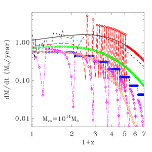
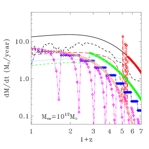
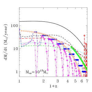
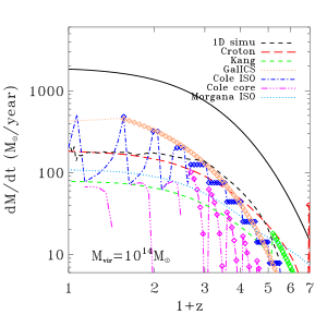
Figure 1: The cooling rates of dark matter haloes with a smooth, averaged accretion history. The panels show results with different final virial masses ($10^{11},10^{12},10^{13}$ and $10^{14}\>{\rm M_{\odot}}$) as labeled. The solid line denotes the rate at which baryons accrete into the dark matter halo. Each of the other lines denotes the cooling rate predicted by a cooling algorithm, as noted in the upper-right corner of the forth panel (see text). The segments of the lines covered by diamonds represent the “rapid” cooling regime and the plain lines represent the “slow” cooling regime. (See §2 for the cooling regime identification in each model.) Note that the MORGANA model does not differentiate the cooling regimes.

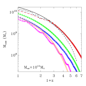
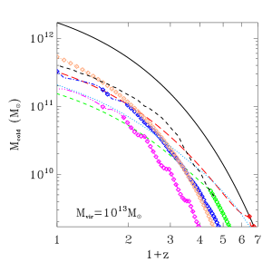
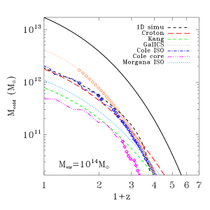
Figure 2: The accumulated cold gas mass in the central galaxy for the same model as Fig. 1, using the same halo masses. The solid lines plot the total mass of baryons in the dark matter halo. The black dashed lines plot the spherically symmetric simulation results.

Figures 1 and 2 show the predicted cooling rates and the accumulated cold gas masses, respectively. In these plots, we denote cooling in the “rapid” regime by diamonds and that in the “slow” regime by lines. The black short-dashed line in each panel shows the result of the spherical simulation. As one can see, in all the models, low-mass haloes and high-redshift haloes are dominated by “rapid” cooling while massive haloes at low redshift tend to be dominated by the “slow” cooling phase. However, since different models have different criteria for the cooling modes, the predicted transition times between these two cooling regimes are very different in the different models, and the halo masses at the transition can vary by almost two orders of magnitude. Thus, the transition mass in SAMs in general does not correspond to a given halo mass scale where shock heating of the gas becomes important (see also discussion in Appendix of Kereš et al., 2005).

The different models predict different cooling histories for the same dark matter halo. Since the Croton, Kang, and GalICS models redistribute the gas at every time step, and since the gas supply in the smooth-accretion halo model is continuous, these three models predict smooth cooling histories in both the “rapid” and “slow” cooling regimes. Since the Croton model accretes all the halo gas onto the central galaxy when the halo is in the “rapid” mode, the cooling rate follows the halo accretion rate in the early history of the halo. When haloes are in transition to the “slow” cooling regime, however, the accretion rate fluctuates as the haloes switch modes in adjacent time steps (see §2). In the Kang model, there is a factor of two drop in the cooling rate at this transition, as expected from their parameterisations (also see §2). The Croton model predicts a higher cooling rate than the Kang model, because the former assumes a shorter timescale for gas cooling. However, the reduced cooling in the Kang model leaves more gas in the halo, which enhances the cooling rate ($\propto m_{gas}^{2}$), thereby reducing the difference between the two models. This explains why the predicted total amounts of cooled gas for low-mass haloes in these models become more similar at late times.

Since the gas distribution is reset when the halo mass is doubled in the Cole model, the gas supply is not continuous. Thus, the cooling rate shows discrete features after every halo birth time. If one replaces the gas distribution with a singular isothermal density profile in the Cole model, the gas suddenly forms a central density cusp every time the halo mass doubles, boosting the cooling rate. When a halo is in the “rapid” cooling regime, the free-fall time determines the cooling rate. Hence, in the singular isothermal profile case, the cooling rate remains constant until the halo doubles its mass and the free-fall time changes. However, when the halo is in the “slow” cooling regime, the cooling radius determines the cooling rate, and the cooling rate drops with time owing to the decrease in the local gas density. When a core is added to the halo gas density distribution and the halo gas is redistributed when the halo mass doubles, the cooling rate then drops because the central gas density is low and the time interval $t-t_{\rm form}$ available for the hot halo gas to cool in the newly formed halo is short. However, as the cooling radius marches outwards, the local density approaches that of the singular isothermal density profile and the cooling rate approaches that seen in the model without a core. For very massive haloes with a cored gas density profile, the cooling rate can be very low owing to their high temperatures and low central densities (also see Viola et al., 2008).

If the GalICS model adopted an singular isothermal gas profile, its cooling rate would follow the upper envelope of the core-free Cole model prediction. Since the model has a small core radius, the predicted cooling rate is right between the Cole models with and without a core. This is not surprising given that the GalICS model adopts the same formula to predict the cooling rate as the Cole model right after a halo doubles its mass, as discussed in §2.5.

Since the MORGANA model does not distinguish the “rapid” and the “slow” cooling regimes, in Figure 1 and 2 we only plot the predicted total cooling rates and cold gas masses (the light blue dotted lines). The model, with the assumption of an isothermal gas profile, generally predicts higher cooling rates at early times for all halo masses. This characteristic has also been pointed out by previous studies using static halos and realistic gas profiles (Viola et al., 2008). At late times, the predicted cooling rates of the MORGANA model for an isothermal profile are about 1.4 times higher than those of the Kang model, which is the closest to the classic White & Frenk (1991) model among the models. This is in an excellent agreement with the analytic solutions of the two models for the isothermal gas profile presented in the appendix of Viola et al. (2008), (also see Bertschinger, 1989; Keres, 2007, for a more detailed discussion).

To compare with the Somerville model, one might consider assigning the halo lifetime as the Hubble time, rather than the time to the last merger. Without major mergers and because halo gas cools efficiently at high redshift, the model would predict that all the accreted gas would cool in a halo regardless of its mass. Without a new halo “birth time” to redistribute the gas, the model would always add the newly accreted gas to a thin shell between the cooling radius and the virial radius. Therefore, the halo gas density would remain high and cool efficiently throughout its lifetime.

As seen in Figure 2, for the two lower-mass haloes, the total cold gas masses predicted by all the models are within a factor of about 2 of each other at the present time. The differences increase with mass and are the largest for the $10^{14}\>{\rm M_{\odot}}$ halo. For these massive haloes, the GalICS model predicts the largest amount of cold gas; the Cole model without a core and the Croton model are in the middle; and the Cole model with a core and the Kang model predict the smallest amounts. Although the cooling rates predicted by the two Cole models look very different from the other models owing to their discontinuous behaviour, the total cold gas masses predicted by the Cole model without a core for haloes with masses $10^{12}$–$10^{14}\>{\rm M_{\odot}}$ are quite close to the predictions of the Croton model. For the two intermediate mass haloes, the total cold gas mass predicted by the GalICS model closely tracks that of the Cole model without a core over all redshifts, but for the higher mass haloes the cold gas mass predicted by GalICS model is larger than that of the Cole model at redshifts $z\la 2$. Compared with the spherically symmetric, hydrodynamic simulation, all the models under-predict the cooling rates for small haloes at late times, with only the Croton model approaching the simulation result. For massive haloes, the Croton and Cole models without a core are consistent with the simulation in the “slow” cooling regime.

3.2 Cooling in Merging Haloes

Cold dark matter haloes form hierarchically through both accretion and the merging of smaller structures. Therefore, the models presented in the previous section, which are based on the assumption of smooth accretion, do not fully capture the realistic picture of gas cooling in CDM haloes. In this section, we incorporate the different cooling algorithms into merger trees to show the performance of these algorithms under more realistic conditions.

Halo merger trees can either be extracted from $N$-body simulations or generated using Monte-Carlo methods. Because merger trees from N-body simulations contain information about both halo dynamics and environment, they have been widely adopted lately for modelling galaxy formation. However, Monte-Carlo merger trees, which lack this information, are still a powerful alternative as they are much easier to generate and have infinite resolution in principle. In this section, we adopt Monte-Carlo merger trees generated with the algorithm recently developed by Parkinson et al. (2008). This algorithm was tuned to match the conditional mass functions from $N$-body simulations. For a simple, illustrative example, we choose the free parameters in the model so that the resulting halo conditional mass function matches the EPS conditional mass function, i.e. $G_{0}=1$ and $\gamma_{1}=\gamma_{2}=0$ (see Parkinson et al., 2008). The virial radius of a halo is defined so that the mean over-density within it is a factor $\delta_{\rm vir}$ times the critical density of the universe. We use the fitting formula by Bryan & Norman (1998) to calculate $\delta_{\rm vir}$. This definition of virial radius is also the same as that used in the simulations presented in this paper.

As in the previous section, we study four cases, with halo masses of $m_{\rm vir}=10^{11},10^{12},10^{13}$ and $10^{14}\>{\rm M_{\odot}}$ at the present time. It is worth noting that the main difference between the merger tree model and the smooth accretion model is that gas can cool in all progenitor haloes in a merger tree but only cool in the main branch haloes in the smooth accretion model. To make a fair comparison with the results obtained in the last subsection, we only look at the main branch of the halo merger trees. The cooling histories of different haloes can be very different even if they have the same final mass because for different haloes mergers occur at various times and with different progenitor mass ratios. To sample the cooling histories, we generate 100 merger trees for each final halo mass and average the results. We set the mass resolution (the minimum halo mass tracked by the merger tree) to be 0.001 times the final mass of the halo. We store merger trees at 60 redshifts that are equally spaced in $\log(1+z)$ from $z=6$ to $z=0$. We will test the effects of the choice of mass and time resolution on the predicted cooling histories, and demonstrate that our results are numerically robust to these choices.

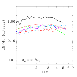
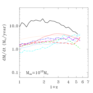
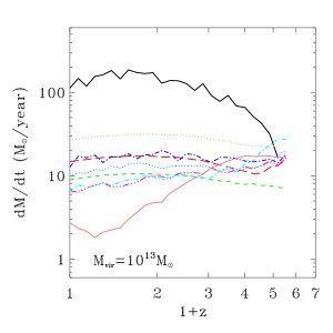
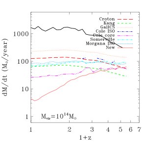
Figure 3: The cooling rate as a function of redshift for the Monte Carlo generated merger tree SAMs. The panels use the same final halo masses as the previous figures. For each halo mass, 100 merger trees are generated and the results are averaged. Only the cooling within the main branch haloes is shown. The solid line denotes the average baryon accretion rate of the haloes. The other lines correspond to the cooling rates predicted by the different cooling models as shown in the legend.

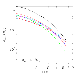
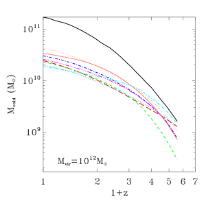
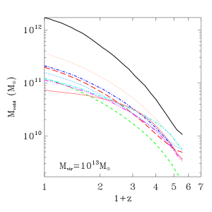
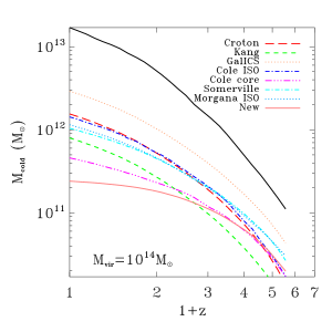
Figure 4: The cumulative cold gas mass of the central galaxies for the merger model in Figure 3 as a function of redshift. Only the gas cooled in the main branch is shown.

We illustrate the cooling rates and cold gas masses (both being the average of 100 merger trees) of the main progenitors for the four halo masses in Figures 3 and 4. Unlike the models with smooth MAHs, the central galaxies in the merger tree models could have a considerable fraction of their cold gas mass acquired through merging satellite galaxies. To exclude any differences that could result from the different treatment of galaxy mergers in the SAMs and to concentrate our study on the cooling of the halo gas, we exclude all the cold gas mass acquired through mergers from our analysis. Even with this treatment, gas cooling in progenitors can still have an important effect because it lowers the amount of gas available for cooling in the descendant haloes. Remember that the cumulative cold gas mass shown in Figure 4 represents the result of cooling that occurs only in the main branch.

The figures show some of the same features seen in the simple smooth-accretion model, but some new features arise owing to the merging nature of the dark-matter haloes. First, the amounts of cumulative cold gas shown in Figure 4 are smaller than the corresponding results shown in Figure 2, owing to the excluded gas that cooled in merging progenitors. Second, the cooling rate in the Croton model remains higher than in the Kang model, but for small haloes the differences between the two models are reduced since the Croton model switches to “slow” cooling at earlier times than the Kang model. This occurs for small haloes because the switch between cooling regimes almost always occurs at a time when the halo mass is about $3\times 10^{10}\>{\rm M_{\odot}}$ for the Croton model and about $2\times 10^{11}\>{\rm M_{\odot}}$ for the Kang model, as shown in Figure 2. For the lowest mass haloes ($10^{11}\>{\rm M_{\odot}}$), the Croton model predicts a higher cooling rate at high redshift, but this leaves less hot gas to cool at lower redshift. In contrast, the Kang model leaves more gas to cool at low redshift, leading to higher cooling rates at late times in these low mass haloes. Third, the MORGANA model for an isothermal profile predicts lower cooling rates than the Kang model for the hierarchically growing halos. This seems contradictory to what we find in the case of smooth-accretion halos, where the cooling rates predicted by the MORGANA model are higher than the Kang model. A similar behaviour is also shown in De Lucia et al. (2010), in which the authors compared the MORGANA model with the Croton model and the Durham model and, against their expectations, they found that the MORGANA model does not predict more efficient cooling than the Croton model. This result seems surprising, but it is easy to understand when the hierarchical formation of dark matter halos is taken into account. As we have shown, the MORGANA model cools faster at early times in progenitor halos, the main branch halo at later times has less hot gas to cool and, therefore, has a lower cooling rate. Fourth, adding a central core to the gas density distribution in the Cole model yields lower cooling rates for massive haloes, yet it does not have a significant effect on low-mass haloes because the cooling in these haloes is so efficient that most of the gas can cool even if the gas density is lowered by the presence of a core. Finally, the GalICS model in general predicts cooling rates that are higher than any of the other models.

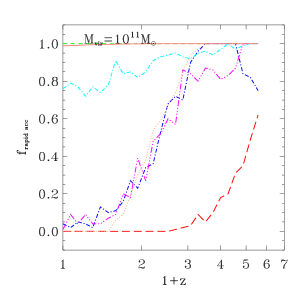
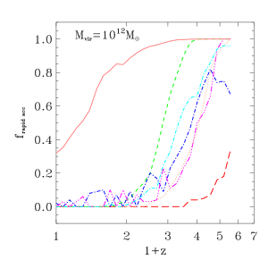
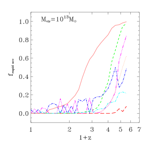
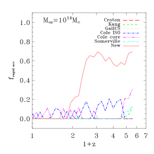
Figure 5: The fraction of main branch haloes in the “rapid” accretion mode as a function of redshift for the merger model used in Figure 3.

In the SAMs considered here, except the MORGANA model, a halo is either in the “rapid” or the “slow” cooling mode. However, haloes with the same final mass may switch between the modes at different times owing to their individual merging history. Figure 5 show the fraction of haloes in the “rapid” mode as a function of redshift for haloes of different final masses, as predicted by the cooling models. This fraction is determined from a limited halo sample at each redshift snapshot and is somewhat noisy. Nevertheless, several features can be seen from the figure. For small haloes “rapid” mode accretion dominates during the entire formation history in the Kang model and the Somerville model, while the other models switch to “slow” mode at $z\sim 2$. The intermediate mass haloes all have transition from the “rapid” mode to the “slow” mode at some time during their formation histories but the transition occurs at different times in the different models. The transition times predicted by the Croton model and Kang models are consistent with the prediction of the simple smooth accretion model presented above, but the GalICS model and the two Cole models predict transition times that are different from the smooth accretion model. As discussed in §2, the definition of “rapid” and “slow” modes for the GalICS model depends on the time step, which differs between the smooth-accretion and merger tree models, and so the difference in the predicted transition times is not surprising. In the Cole models, since the gas distribution is reset whenever the halo doubles its mass, the results can be sensitive to the details of the halo assembly history. Finally, for massive haloes, all the models predict that “slow” mode accretion dominates through their entire formation history. The Croton model has the smallest fraction of haloes in the “rapid” mode at any redshift and mass, making this accretion mode the least important in their model. However, models that do not renormalise the gas density profile at every time step often have some small fraction of haloes in the “rapid” mode even at late times and for massive haloes.

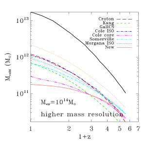
Figure 6: Mass and time resolution tests of SAMs shown as the cumulative cold gas mass of $10^{14}\>{\rm M_{\odot}}$ halos. The left panel shows the predictions with a merger tree mass resolution five times higher than that for the lower right panel of Fig.4. The right panel shows the predictions using merger tree time steps that are two times larger.

The mass resolution adopted for these merger trees is 0.001 of the final halo mass. For the two lower masses, this choice achieves higher mass resolution than those adopted in the literature. For the $10^{13}\,\rm M_{\odot}$ halos, the resolution is similar to that of the models based on the Millennium simulation (Springel et al., 2006). The mass resolution for the $10^{14}\,\rm M_{\odot}$ halos is lower than what is typically used in SAMs. We notice that, for some models at very high redshift, the predicted cold gas mass is not much higher than the adopted mass resolution, which suggests that these results are likely affected by the finite resolution of our model. To test the effect of mass resolution on our results we generate the same number of merger trees with a final mass of $10^{14}\,\rm M_{\odot}$ using a mass resolution of $2\times 10^{10}\,\rm M_{\odot}$. This mass resolution is 5 times higher than the one used in our previous discussion. We keep everything else the same and run the models on the merger trees. The left panel of Figure 6 shows the predicted cold gas of the central galaxies as a function of redshift. We find that increasing the mass resolution has no effect on the accretion histories at early times, indicating that the mass resolution we adopt can well resolve the accretion of these halos even at early times when the halo mass is low. At late times, however, the predicted cold gas mass shows a mild deviation from the fiducial models. The high resolution models predict lower cold gas mass. In the most extreme case, the GalICS model, the cold gas mass is reduced by 1/3, and the decrease is smaller for the other models. Although the decreases in the cold gas mass at late times are not significant, the effect is systematic. This occurs because with a higher mass resolution, more gas mass cools in progenitors instead of in the main branch halos and hence less gas mass is available to cool in the main branch halos at later times. The relative behaviour between the models, however, stays the same, confirming our previous discussion. We also test the effect of the time resolution of the merger trees. For the $10^{14}\,\rm M_{\odot}$ halos, we use the same merger trees, but only save 30 snapshots between $z=0$ and 6, instead of 60, so that the time resolution is reduced by a factor of 2. We run the models on the reduced trees and show the results in the right panel of Figure 6. The predicted cold gas mass is stable and not sensitive to the choice of time steps, except at very early times, $z>4$.

3.3 Comparison to Numerical Simulations

In this section, we compare the SAM results for cooling in merging haloes with a large-box cosmological Smoothed Particle Hydrodynamics (SPH) simulation (Kereš et al., 2009b). The simulation models a 50$\>h^{-1}{\rm{Mpc}}$ comoving, periodic cube using $288^{3}$ dark matter and $288^{3}$ gas particles, i.e. around 50 million particles in total. The mass of each gas and dark matter particle is $9.0\times 10^{7}\,\rm M_{\odot}$ and $4.4\times 10^{8}$, respectively. Hence, $\sim 10^{11}\,\rm M_{\odot}$ halos in the simulation are typically composed of about 200 gas and 180 dark matter particles. There are a larger number of gas particles because the baryon fraction has about a 10% excess over the cosmic average value for small halos, but converges to the cosmic baryon fraction for massive halos (Keres, 2007; Faucher-Giguere et al., 2011). However, since haloes of these small masses accrete their gas through cold mode accretion, to recover the converged gas accretion rates it is only necessary to correctly reproduce the gravitational gas accretion rate, something that is easily accomplished using this many particles. Gravitational forces are softened using a cubic spline kernel of comoving radius $10\>{h^{-1}{\rm kpc}}$, approximately equivalent to a Plummer force softening of $7.2\>{h^{-1}{\rm kpc}}$. The virial radius of the small halos ($\sim 10^{11}\,\rm M_{\odot}$) is $121\>{\rm kpc}$ at $z=0$, which means that the gravitational softening is about 1/12 of the virial radius. For massive halos ($\sim 10^{13}\,\rm M_{\odot}$), the softening is less than 1/50 of the virial radius at $z=0$. The initial conditions are evolved using the SPH code, Gadget-2 (Springel, 2005). This code uses the entropy and energy conserving formulation of SPH from Springel & Hernquist (2002), which avoids numerical problems with hot gas over-cooling in massive haloes (Springel & Hernquist, 2002; Keres, 2007). Our version of Gadget-2 includes modifications to incorporate gas cooling, a photoionising UV background, and star formation. We include all the relevant cooling processes with primordial abundances as in Katz et al. (1996), similar to the cooling implementation in the SAMs. We do not include any metal enrichment or cooling processes associated with heavy elements or molecular hydrogen. This simulation also includes a spatially uniform, extragalactic UV background that heats and ionises the gas. The background flux first becomes nonzero at $z=9$ and is based on Haardt & Madau (2001); for more details see Oppenheimer & Davé (2006). The UV background pre-heats the gas and modifies the cooling curve, but this change affects only galaxies far below the resolution limit of the simulations at early times, growing to around the resolution limit only at late times. Our tests show that incorporating the UV background and the cooling function used in the simulation do not significantly affect the accretion rates and the mass accumulation history of SAMs presented in this paper, although the transition from rapid to slow cooling regime can be affected in some models (see Kereš et al., 2005). When the UV background is included, cooling in small progenitor halos is suppressed and, therefore, the more massive descendant halos will have more hot gas. As a result, the addition of a UV background results in slightly higher accretion rates. Our tests show that the accretion rates of the $\sim 10^{11}\,\rm M_{\odot}$ halos in SAMs are enhanced by less than 20% when the UV background is included. For more massive halos, the effect becomes even smaller. The simulation also includes the star formation prescription and the sub-resolution two-phase medium, which is pressurised by supernovae, following the formalism of Springel & Hernquist (2003). However, since supernova winds are not explicitly included in this simulation, star formation and the supernova pressurised two-phase medium does not affect any halo gas, i.e. it only affects gas within the galaxies themselves, and hence is irrelevant for the comparisons we present here. Since the simulation and the SAMs differ in their star formation modelling, we compare them using the total baryonic masses of the galaxies, adding together the stellar and cold gas components.

To identify bound groups of cold, dense baryonic particles and stars, which we associate with galaxies, we use the program SKID (see Kereš et al., 2005 for more details). Briefly, a galaxy identified by SKID contains bound stars and gas with an over-density $\rho/\bar{\rho}_{\rm baryon}>1000$ and temperature $T<\mbox{30,000 K}$. Here, we slightly modify this criterion and apply a higher temperature threshold at densities where the two-phase medium develops. Such a modification is necessary to allow star forming two-phase medium particles to be a part of a SKID group, since at high densities the mass-weighted temperature in the two phase medium can be much higher than 30,000 K. To identify haloes, we use Spherical Overdensity (SO) algorithms with the algorithm and virial overdensity as in Kereš et al. (2005), adjusted to the new cosmology. We define “central” galaxies simply by choosing the most massive galaxy in each halo, regardless of position.

To avoid counting the accretion of sub-resolved groups as smooth accretion, we define smooth gas accretion as the accretion of gas particles that were not part of any SKID identified group at the previous time. In practise, this procedure will avoid counting sub-resolution mergers down to galaxies with $\sim 20$–30 particles, i.e. baryonic galaxy masses of $\sim 2\times 10^{9}\>{\rm M_{\odot}}$, approximately the mass where the galaxy mass function in our simulation drops rapidly owing to our limited resolution. Readers are referred to Kereš et al. (2009b) for a more detailed description of the simulation. There, the authors discuss that a large fraction of the cold-mode accretion in haloes more massive than $\sim 5\times 10^{12}\>{\rm M_{\odot}}$ at late redshifts is contributed by “cold drizzle”, i.e. accretion of individual cold particles or small groups of particles below the resolution limit that might be a consequence of poorly understood numerical effects. In this comparison, we still keep the contamination of “drizzle” as there is no unique way to remove it.

To make a fair comparison between the SAMs and the simulation, we generate a set of merger trees with the same cosmological model, the same volume, and the same mass resolution as the simulation using the Monte-Carlo method. We then run all the SAM cooling models for these halo merger trees to predict the cooling rates and the total cold gas masses. A comparison between the simulation and the SAM using merger trees from the simulation itself might be more direct, but for the purposes of this study, the Monte-Carlo merger trees are sufficient and better facilitate comparisons with the previous sections. We first draw a random sample of dark matter haloes using the EPS halo mass function from a $(50\>h^{-1}{\rm{Mpc}})^{3}$ volume for the same cosmological model as the simulation. We only generate the merger trees for haloes with virial masses larger than $5\times 10^{10}\>{\rm M_{\odot}}$ at $z=0$ for the sample, and we set the halo virial mass resolution to be $2\times 10^{10}\>{\rm M_{\odot}}$ to be approximately consistent with the effective resolution of the simulation. The time step of the merger tree is chosen to be the same as that used in §3.2. We apply every SAM cooling model to the merger trees and compare the SAM predictions with the simulation.

To avoid the complication of tracing the main branch of the halo merger trees in the simulation, unlike in the previous sections, we look at haloes in a fixed mass range at different redshifts. At each SAM or simulation snapshot, we select haloes in the mass ranges $10^{11\pm 0.15}\>{\rm M_{\odot}}$, $10^{12\pm 0.15}\>{\rm M_{\odot}}$, and $10^{13\pm 0.20}\>{\rm M_{\odot}}$. We then calculate the cold gas accretion rate for central galaxies in these haloes and the total halo gas mass that has not collapsed onto any galaxies, centrals or satellites, in the haloes for both the simulation and the SAMs. For the simulation, we choose four snapshots at $z=0$, 1, 2, and 3, and determine the accretion rates in each of these snapshots using the change of the cold gas mass between $z$ and $z+0.1$. For the SAMs, we use 15 snapshots evenly distributed in $\log(1+z)$ from $z=6$ to $z=0$.

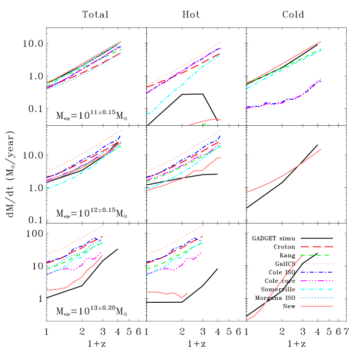
Figure 7: The average gas accretion rate onto the central objects of haloes with different halo mass ranges noted in the left panels as a function of redshift. The first column shows the total accretion rate; the second column shows the “hot” accretion rate; and the third column shows the “cold” accretion rate. The solid black lines show results from the SPH simulation, while the colour coded lines show the predictions of the SAM cooling models. Halo mass range is held constant with redshift.

For each halo mass range, we plot the averaged cold gas accretion rate of the central galaxies as a function of redshift in each row of Figure 7. For the simulation, each of the three columns shows the total accretion rate, the accretion rate in the hot mode and the accretion rate in the cold mode, respectively. As in the previous section, we do not include any cold gas from merging satellite galaxies in the SAMs. Correspondingly, in the simulation, we define the gas accretion as the accumulation of gas that was outside of any galaxy at the previous simulation output. We show the cooling rate from the hot halo gas in the simulation in the middle column. Since haloes may accrete cold gas directly, any cold gas that collapses onto the central galaxies but is not associated with merging galaxies is accounted as cold-mode accretion and plotted in the last column. The SAMs do not explicitly model the cold halo gas component, so the entire gas accretion is simply defined as the gas mass that cools from the hot halo and collapses onto the central galaxy. However, it is generally believed that the “rapid” and “slow” mode cooling in SAMs are proxies for the cold and hot-mode accretion observed in simulations. Following this idea, we split the accretion in SAMs according to the definition of the “rapid” and “slow” cooling mode for each of the models and plot them in the corresponding columns to compare with the simulation.

These plots illustrate several interesting points. We find that the SAMs have considerable differences in their predicted cooling rates, both in total and in the different modes, following the patterns seen in previous sections. For $\sim 10^{13}\>{\rm M_{\odot}}$ haloes, the predicted accretion rate differs by up to a factor of 4. Compared with the simulation, we find that none of the SAMs predicts cooling rates consistent with the simulation for all halo masses. For $10^{11}\>{\rm M_{\odot}}$ haloes, where the cooling is efficient at all redshifts, the cooling rate is strongly limited by the halo baryon accretion rate which is the same for all the SAMs, so the predicted cooling rates do not differ very much. However, the split between the accretion modes does not agree with the simulation, where galaxies in small haloes accrete gas mainly through cold accretion, which approximately follows the infall of baryons into haloes (see Kereš et al., 2005). In contrast, SAMs predict a much higher accretion rate through “slow” cooling. As shown in the predictions of SAMs, the rate of “slow” mode cooling makes up for the cold-mode accretion in small haloes, which occurs in the simulation but is missing in those models. Moreover, it is clear that most of the SAMs, except the Somerville and GalICS models, still under-predict the total accretion rate for small haloes even though they predict much faster cooling of hot gas than the simulation. For $10^{12}\>{\rm M_{\odot}}$ haloes, the total accretion rates over redshifts predicted by the SAMs show the same trend as the simulation, and the amplitudes are close to the simulation within a factor of 2–3. However, the models attribute all the accretion to the “slow” accretion, which results in zero “rapid” mode accretion and an over-prediction of hot mode accretion at high redshift. For $10^{13}\>{\rm M_{\odot}}$ haloes, the cooling rates predicted by the SAMs are at least 3 times higher than the simulation results, largely owing to the wrongly assumed steep gas density profile, and again none of the SAMs predict any cold or “rapid” mode accretion in this halo mass bin. (One should be cautious about the discrepancy in cold accretion rates in massive haloes owing to the previously mentioned concerns that the cold “drizzle” in simulated massive haloes might be purely of numerical origin.) In summary, these results indicate that without modelling the cold halo gas, SAMs generally under-predict the cold-mode accretion and over-predict cooling in the hot accretion phase. As a result, the SAMs over-predict the cooling at the high-mass end.

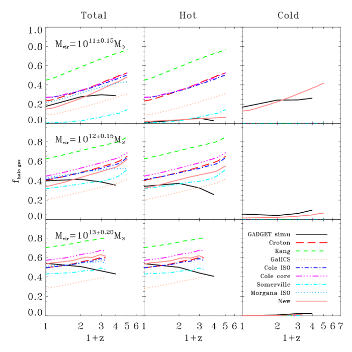
Figure 8: The total uncollapsed, hot and cold halo gas fractions as functions of redshift predicted by different SAMs compared with fractions of the corresponding components in the simulation.

The accumulated total baryonic mass of the central galaxy is difficult to compare between simulations and SAMs, because much of this mass comes from the merging of satellite galaxies. This happens naturally in simulations but depends on the model recipe for dynamical friction in the SAMs, including such parameters as the assigned Coulomb logarithm and tidal stripping, models of which have large uncertainties (Hopkins et al., 2010; De Lucia et al., 2010). To avoid these problems, we focus on the uncollapsed gas mass, comprising both the total hot gas mass and the cold gas that is contained by a halo but is not associated with any galaxies identified by SKID. We compare the averaged uncollapsed gas mass fraction, i.e. uncollapsed halo gas mass divided by the total baryonic mass in the halo, for each halo mass bin from all the simulation to the averaged total halo gas mass fraction from the SAMs. The first column in Figure 8 plots this quantity versus redshift. Similarly, the second column shows the hot halo gas mass fraction, and the third column shows the cold halo gas fraction. None of the models predict any cold halo gas, simply because this component is not included in any of the models. The models show a large variation in their uncollapsed gas fraction. Most of the models predict higher gas fractions than the simulation, because they generally predict less cooling for small haloes at high redshift. The exceptions are the Somerville and GalICS models, which cool most of the halo gas to build up the central galaxies and turn out to predict less uncollapsed gas mass for all halo masses. The simulation shows that cold halo gas contributes a significant fraction of the halo gas in small haloes. Although the hot halo gas dominates for more massive haloes, the simulation shows a mild increase in cold halo gas fraction with redshift for all halo masses.

All the SAMs predict that the hot fraction in haloes of a given mass increases with increasing redshift, in contrast to the weak decrease of the hot fraction with increasing redshift seen in the simulation. For a given virial mass, haloes at high redshifts have higher densities than at low redshifts, so they would cool faster. However, the temperature is higher and the timescale allowing the gas to cool is shorter at high redshifts, which can compensate for the density increase and make cooling slower. The key factor that determines which effect dominates is the dependence of the cooling rate on temperature. If the cooling rate is an increasing function of temperature, such as in the Bremsstrahlung regime, the increase in density with redshift can compensate for the higher virial temperature and the shorter timescales and can result in a higher fraction of cooled halo gas. If the cooling rate drops more rapidly with temperature than $T^{-1/2}$, the increase of the virial temperature with redshift can overcome the increasing density and hence result in less cooling at higher redshifts. In all the SAMs, we find that even for massive haloes, most of the gas actually cools at a temperature below $10^{5}$K, i.e. the bulk of the cooling occurs in small progenitors. For this temperature range, one can expect that the same mass haloes can cool more baryons at late redshifts, which is consistent with what we find in the SAMs. The simulation, however, shows the opposite trend. The cooling and gas mass assembly is more complex in simulations which can cause deviations from the trend predicted by the SAMs. The most important difference between the SAMs and the simulation is the large accretion rate of satellite galaxies at high redshift. These rates are comparable to the central galaxies of the same mass, which makes gas depletion in high-redshift haloes faster (Kereš et al., 2009a; Simha et al., 2009). Even though some satellites can also accrete gas at low redshift, these rates are typically lower than for central galaxies and, therefore, its effect is much weaker. In addition, the UV background can prevent the collapse of baryons into more massive haloes at late time. At high redshift the affected mass is below our resolution limit. But at low-$z$ this mass is close to our resolution limit (Keres, 2007). This can increase the fraction of uncollapsed material during the hierarchical build-up of the descendant haloes. Both of these effects can contribute to produce a flatter, or even reversed trend of uncollapsed fraction with redshift.

To summarise, gas accretion in SAMs differs significantly from accretion in a cosmological hydrodynamical simulation. The intrinsic differences between SAM cooling recipes show up as wide dispersions in the SAM results at all masses and redshifts, either in the accretion rates or uncollapsed gas fractions or both. Galaxy formation through accretion of cold gas is important in the simulations but is not modelled at all in SAMs. SAMs assume that all the gas virialises as soon as it enters the halo. The “rapid” mode accretion, which is sometimes taken as a proxy for cold mode accretion generally has lower rates than the simulated cold mode rates. However, the lack of cold-mode accretion is partially compensated for by more efficient cooling of the hot halo gas. This reduces the discrepancy between total accretion rates in the simulation and the SAMs in small and intermediate mass haloes. However, a large discrepancy remains at the high-mass end where hot-mode cooling dominates.

4 A New Model

As demonstrated in numerical simulations (Kereš et al., 2005; Keres, 2007; Kereš et al., 2009b), cold-mode gas accretion plays an important role in low-mass haloes at all redshifts and in massive haloes at high-redshift. Although current SAMs include a cooling-radius-based “rapid” mode which may mimic the cold-mode accretion to some extent, they do not model the co-existence of cold and hot halo gas and the bimodal accretion seen in the simulations. Motivated by the bimodal accretion in simulations, we propose a phenomenological model that explicitly incorporates cold-mode accretion. We introduce a cold gas component associated with dark matter haloes that evolves separately from the hot halo gas. This gas is assumed to avoid shock heating during infall and it is not hydrostatically supported. Furthermore, since cooling is not relevant for this component, it is assumed to be accreted by the central galaxy in a free-fall timescale unless the host halo merges into another halo. We continue to track the hot component, whose evolution in a halo is assumed to follow the radiative cooling described in §2. SPH simulations (Kereš et al., 2009b) have shown that the majority of massive haloes develop large cores in their hot gas distribution, presumably caused by the dynamical heating of recent mergers. To model this effect we link the size of the gas core to the mass assembly of the host dark matter halo, so that the cooling rate for recently formed massive haloes is reduced.

We describe the “bimodal” nature of cold gas accretion by the cold and hot halo-gas fractions. SPH simulations (Kereš et al., 2005; Dekel & Birnboim, 2006; Keres, 2007; Ocvirk et al., 2008; Kereš et al., 2009b; Brooks et al., 2009) show that these fractions depend on both redshift and halo mass. In addition, the bimodal accretion has a sharp transition at a nearly fixed halo mass over a wide redshift range. Guided by these simulation results, we model the fraction of hot halo gas for a given virial mass, $m_{\rm vir}$, as an error function:

$$p_{\rm hot}(m_{\rm vir},z)={f_{m}(z)\over 2}\left[1+\rm{erf}\left({\log m_{\rm vir}-\log m_{\rm tran}\over\sigma_{\rm logm}}\right)\right],$$ (24)

where $m_{\rm tran}$ is the transition mass, $\sigma_{\rm logm}$ characterises the sharpness of the transition, and $f_{m}(z)$ describes the maximum hot halo gas fraction for a halo with $m_{\rm vir}\gg m_{\rm tran}$ at redshift $z$. Simulations show that the accretion in massive haloes is dominated by the hot mode at low redshifts but the contribution of the cold mode increases with increasing redshift. We therefore model $f_{m}$ as a decreasing function of redshift,

$$f_{m}(z)=f_{\rm c}e^{-({z\over z_{\rm tran}})^{2}}+\left(1-f_{\rm c}\right),$$ (25)

where $z_{\rm tran}$ is a transition redshift and $f_{\rm c}$ is the fraction of the cold halo gas in very massive haloes at $z\gg z_{\rm tran}$. Our model for hot gas fraction, therefore, is specified by three free parameters. We fix the values of these parameters by matching the model predictions with the accretion rate and halo gas fraction (in both the cold and hot modes) obtained from the simulations. This gives $m_{\rm tran}\approx 10^{11.4}\>{\rm M_{\odot}}$, $\sigma_{\rm logm}\approx 0.4$, $z_{\rm tran}=4$ and $f_{\rm c}=0.1$.

This parametrisation serves only as an illustration that bimodal accretion matching a particular simulation can be modelled and straightforwardly implemented in SAMs. A general treatment must be based on a physical model for the dependence of the cold and hot gas fraction on the resolution, metal cooling, halo assembly history, and feedback processes. Each of these effects can change the relative distribution of the hot and cold components.

We apply the above model to merger trees to predict the evolution of the different gas components in a halo by calculating the hot fraction, $p_{\rm hot}$, for a halo of mass $m_{\rm vir}$ at redshift $z$. This fraction of the baryonic mass in the halo is assumed to be at the virial temperature, while the rest is assumed to be in the cold component. To make predictions for the accretion rate of the cold component onto the central galaxy, we assume that the accretion rate is half of the total mass of cold halo gas, $m_{\rm ch}$, divided by the free-fall timescale,

$$\dot{m}_{\rm cold}={m_{\rm ch}\over 2\tau_{\rm dyn}}={m_{\rm ch}V_{\rm c}\over 2r_{\rm vir}}.$$ (26)

Although the cold gas is likely to infall on a timescale close to the free-fall time, we only allow half of the total cold mass to collapse onto the central galaxy in a free-fall time to mimic several effects that are not included in the current model: some of the material can be accreted by satellites, a fraction of the currently cold gas can get heated to the virial temperature, and the angular momentum of the infalling gas must be removed before it can be accreted by the central galaxy.

We redistribute the hot gas only at the birth time of a halo. Following the Cole model, a halo is born when its mass is doubled. Motivated by the simulation results described above, we assume a cored profile for the hot halo gas, with a core radius, $r_{c}$ being half of the scale radius of the halo profile, $r_{s}$ (assumed to have an NFW form, see Navarro et al., 1997), i.e. $r_{c}=0.5r_{s}$. $N$-body simulations have shown that the halo concentration parameter, $c=r_{\rm vir}/r_{s}$, is closely related to the formation time of a halo (Bullock et al., 2001; Wechsler et al., 2002; Zhao et al., 2003a, b, 2009). We adopt the following simple form for this relation:

$$c=3\left({1+z_{c}\over 1+z}\right),$$ (27)

where $z$ is the redshift at selection and $z_{c}$ is the redshift at the birth time. This allows us to estimate $r_{s}$, and hence $r_{c}$, for any halo at any redshift. Using this prescription, we find that $10^{11}\>{\rm M_{\odot}}$ haloes at the present time typically have a concentration of about 15, while haloes of $10^{15}\>{\rm M_{\odot}}$ have a concentration of about 5.

From the hot gas profile, we calculate the cooling radius, $r_{\rm cool}$, and the free-fall radius, $r_{\rm ff}$, and assume that only the hot gas within both of these two radii can cool and accrete onto the central galaxy. Thus, the effective radius for cooling is $r_{\rm min}(t)=\min[r_{\rm cool},r_{\rm ff},r_{\rm vir}]$. The cooling rate of the hot mode is assumed to be equal to the mass of hot gas between spherical shells of radii given by the values of $r_{\rm min}$ at the current time and at one time step earlier. At each generation, the newly accreted hot gas is included by changing the normalisation of the hot gas profile at each time step, following the Somerville model.

Figures 3 and 4 show that the new model predicts higher cooling rates for low-mass haloes, but lower cooling rates for massive ones compared to the other models. In the new model, low-mass haloes accrete gas mostly through cold mode, and massive haloes cool gas from their hot haloes at a reduced rate because they typically form late and hence maintain a big core in their hot gas distribution. Figure 5 shows the fraction of cold accretion predicted by the new model, which is the ratio of the accretion rate of the cold halo gas to the total accretion rate. Clearly, in the new model the cold mode dominates more and the transition from cold to hot modes occurs at lower redshifts.

Figures 7 and 8 compare the new model with the simulation. The new model nicely reproduces the accretion rates for both the cold and hot modes for all halo masses over a large range of redshift and the predicted mass fractions in the hot and cold halo gas are in rough agreement the simulation results. However, as in the other models, the new model also predicts a weak increasing trend for the hot fraction with increasing redshift in contrast to the weak decreasing trend seen in the simulation (see Section 3.3).

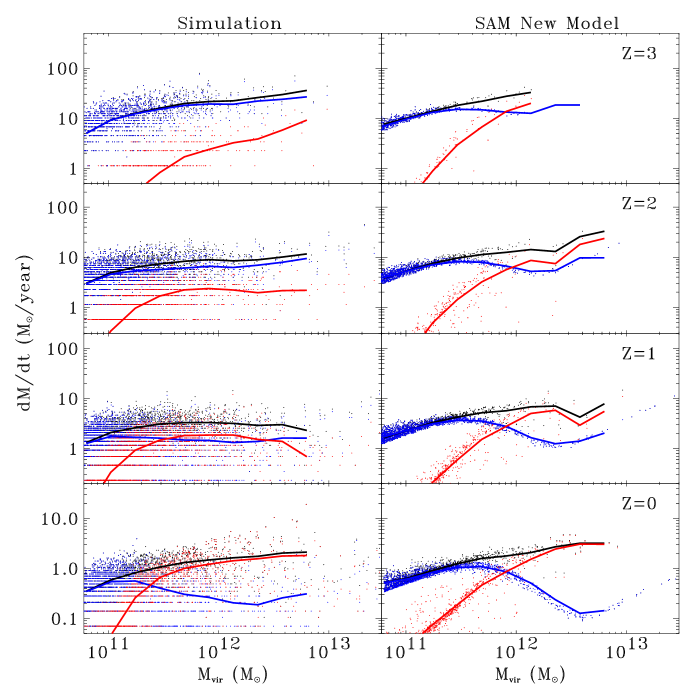
Figure 9: The total rate of accretion (black) and the “cold” (blue) and “hot” (red) mode contribution for individual central galaxies in haloes in the simulation (left column) and the new model (right column) at four redshifts, which are noted in the upper-right corner of each right panel. The red, blue and black lines show the mean hot, cold and total accretion rates.

To compare the new model with the simulation results in more detail, we show the predicted and simulated accretion rates in both the cold and hot modes for individual haloes at four different redshifts, $z=0,1,2$ and 3 in Figure 9. The new model matches the simulation results much better than any other model considered in this paper. In particular, the model shows the cold–hot-mode transition at $\sim 7\times 10^{11}\>{\rm M_{\odot}}$. Although the transition mass has a complex redshift dependence in the simulation, the model captures the characteristic mass scale. However, the predicted scatter in the accretion rate for a given halo mass is much smaller than that seen in the simulation. For a given merger history, the model ignores all stochasticity that may arise from different merger orbits and from the interactions between different mass components of a halo. The large scatter seen in the simulations suggests that these effects may have a significant impact on the gas accretion rates in individual haloes.

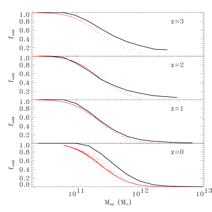
Figure 10: The fraction of cold halo gas in a halo of given mass at four redshifts. Lines show the median of the SPH simulation results, and dots show a randomly selected sample of haloes from the new model SAM.

Figure 10 compares the fraction of cold halo gas for a given halo mass predicted by the new model with that from the simulation. The model reproduces the overall trend seen in the simulation but under-predicts the cold fraction at $z=0$. The discrepancy is a consequence of the temperature criterion used to select cold gas in the simulation. Following Kereš et al. (2005), we demarcate the cold and hot component by $T=2.5\times 10^{5}\rm K$, but this is comparable to the virial temperature for haloes around the transition from mostly cold to mostly hot gas at $z\sim 0$. Therefore, gas in the halo outskirts that is typically slightly colder will be added into the cold component even if a fraction of such gas was shock heated to $\sim T_{\rm vir}$. At high redshift this is not an issue since the $T_{\rm vir}$ of these haloes is much higher.

The new model separately tracks the cold and hot phases of the halo gas. As we have demonstrated in this section, the two-phase model not only reproduces the bimodal accretion seen in simulations of a CDM universe, but also can be tuned to match the simulation results. However, our phenomenological model does not include the physical processes that determine the division between hot and cold halo gas. Therefore, the model parameters presented in this paper apply only when the feedback does not strongly affect the cold-mode accretion we tune the parameters to match a simulation without strong feedback. Feedback and preheating mechanisms may alter the fraction and evolutionary track of the cold halo gas. Further work is needed to better understand the physics of cold-mode accretion (e.g. Oppenheimer et al., 2010), such as the effect of feedback on cold-mode accretion and the interaction between the cold and hot halo gas phases. While our model is purely phenomenological, future physical models need to properly model the change in the accretion rates of cold and hot gas as a function of radius in a halo (e.g. Faucher-Giguere et al., 2011; van de Voort et al., 2010).

5 Discussion and Conclusions

The process of radiative cooling is fundamentally important for modelling galaxy formation. This process is often taken for granted, but, as we have shown in this paper, the predictions of existing cooling prescriptions in semi-analytic models (SAMs) differ significantly. We implemented the numerical recipes used in six published SAM codes, and compared their predictions with each other and hydrodynamic simulations for idealised spherical, smooth-accretion halos and for realistic merging halos in a cosmological context. Our tests examined the central galaxy accretion rates, the total cooled baryonic masses, and the fraction of baryons remaining in a hot halo. We focused on a range of halo masses relevant for galaxy formation and found large variance between different SAMs themselves and between SAMs and the cosmological SPH simulation.

These comparisons are useful for understanding the interdependence of our phenomenological descriptions and illustrate the need for a more reliable cooling model. For example, the cooling algorithms control gas accretion and gas phase fractions, these will affect star formation algorithms, star formation driven feedback, and AGN heating. The discrepancies in the models suggest the possibility of errors in both the physical interpretation and the predictions from SAMs. Furthermore, incomplete or incorrect modelling of the halo gas component will directly affect predictions for properties of halo gas and prospects for direct detection of different gas components.

Although our paper compares the largest collection of SAMs to a hydrodynamic simulation to date, there have been several attempts to compare a single SAM with a SPH simulation (see Benson et al., 2001; Yoshida et al., 2002; Helly et al., 2003; Cattaneo et al., 2007). All of these found good agreement between the “stripped-down” SAMs and the simulations. However, Springel & Hernquist (2002) have shown that the SPH implementation affects gas cooling rates, and as we have seen, subtle choices in SAM implementation may result in dramatic changes in the gas accretion rate. In some cases, we speculate that the reported consensus may be the result of insensitive tests; in others, it may reflect an overzealous match between SPH implementation and the choice of SAM cooling algorithm. Indeed, a recent SAM-simulation comparison (Saro et al., 2010) also shows that the accretion rate of the central galaxies in massive haloes from SAM and SPH simulations differ significantly.

Comparisons between competing SAMs are less numerous in the literature, but a recent paper by De Lucia et al. (2010) compares three models, the “Durham” (effectively Cole with a core), “Munich” (effectively Croton), and MORGANA models (Monaco et al., 2007). These comparisons are complementary to our tests. Their results are similar to ours, e.g. the lower cooling rates in the Durham model in the “rapid” mode at early times and for massive haloes at late times. Moreover, our extended comparison to six SAMs reveals an even larger dispersion among models than that found by De Lucia et al. (2010).

In the absence of strong feedback, most cooled gas in the universe comes from cold-mode accretion where the gas infalls onto galaxies without heating to the virial temperature. This process, therefore, should be central to the cooling models in SAMs. Currently, the “rapid” mode in SAMs is a proxy for this mechanism. However, our study highlights a large variance between the predictions for different SAM implementations. In part, this owes to different cooling radius calculations and timescales for “rapid” mode gas accretion. We also find that SPH simulations predict larger cold-mode accretion rates than the SAM “rapid” mode for some or all halo and redshift regimes, depending on the SAM. In addition, the cooled gas mass in the simulation has an order 30% dispersion, which is much less than that in the “rapid” mode accretion rates predicted by the SAMs. Even in the regimes where the total accretion rates are comparable between the SAMs and simulation, the properties and detectability of the accreting halo gas may very much depend on the accretion mode (e.g. Fardal et al., 2001; Dijkstra & Loeb, 2009; Goerdt et al., 2010; Faucher-Giguère et al., 2010). Furthermore the angular momentum of the infalling material can differ between the accretion modes (Kereš et al., 2005; Benson & Bower, 2010). Different physics of gas accretion in the cold and hot mode clearly needs to be captured properly in a model in order to understand the formation and evolution of galaxies.

To make progress, we propose a new cooling algorithm that introduces the cold-mode gas explicitly. The new model better matches the accretion rates and both the hot and halo gas mass fractions from the simulations. In addition, the explicit cold-mode channel can handle effects like aspherical and simultaneous cold/hot accretion. Other recent work on including cold-mode accretion explicitly in SAMs include Kang et al. (2010), who used a simple sharp transition from cold to hot haloes depending on halo mass, and Benson & Bower (2010), who more closely resembles our gradual transition. Benson & Bower (2010) find that strong SN feedback can always heat the ejected gas to high temperature in the halo and hence argue that the substitution of an explicit cold mode for their “rapid” mode made a negligible difference to their results. Kang et al. (2010) demonstrate that changes in the cold mode are significant for high-redshift, high-mass galaxies, and this impacts the prediction of global star formation rates. The discrepancy between these results suggest that effect of the cold-mode accretion depends on the implementation of feedback (De Lucia et al., 2010). However, the interaction between feedback and the infalling cold gas is not yet clear. High redshift cold-mode accretion proceeds in filamentary streams of cold gas which are hard to destroy by outflowing material, especially because the outflows will tend to expand into the low density regions in the halo. In fact, (Oppenheimer et al., 2010) show that the high redshift cold-mode accretion seems to be insensitive to the gas ejected with milder velocities. Observations that probe the properties of the halo gas could provide constraints on the feedback models and their effect on the cold halo gas. Moreover, it has been pointed out that “preventive” feedback, e.g. radio mode AGN, is unlikely to affect the gas accretion in cold mode with the same efficiency as it would affect gas in a hot halo (Kereš et al., 2009a). Therefore, we would argue that a more accurate treatment for gas accretion in SAMs is crucial to better understand how feedback works in galaxy formation.

This paper demonstrates that cooling processes in current semi-analytic models produce predictions that are at variance with each other and numerical simulations. We advocate a careful normalisation of the cooling models using a combination of numerical simulations and analytic arguments to improve the prescriptions and observational comparisons to constrain the cooling channels. For example, star-formation timescales are expected to be short at high redshift, so the instantaneous star formation rate should provide a lower limit on the ongoing gas accretion. Such observations (e.g. Förster Schreiber et al., 2009) are already providing challenging constraints for cooling models in SAMs (see Khochfar & Silk, 2009). To derive the constraints on gas accretion histories, we have implemented SAMs as a Bayesian inference problem and have demonstrated it leads to genuine constraints on model parameters and on model prescriptions themselves (Lu et al., 2010). For example, the Bayesian approach will allow us to assess the observational support of our new cold-mode accretion prescription relative to the existing cooling prescription using Bayes factors. Alternatively, gas accretion histories may be constrained with one or more observational data sets with non-parametric models (Neistein & Weinmann, 2010). Most likely, a variety of approaches will be necessary to improve our treatment of gas cooling, a key step in understanding how galaxies form and evolve.

6 Acknowledgments

We thank Andrew Benson, Darren Croton, and Martin White for useful discussion. DK acknowledges supports from Harvard University funds and from NASA through Hubble Fellowship grant HSTHF-51276.01-A. This work was supported in part by NSF IIS Program through award 0611948 and by NASA AISR Program through award NNG06GF25G. HJM acknowledges the support of NSF 0908334.

References

- Benson & Bower (2010) Benson A. J., Bower R., 2010, ArXiv e-prints
- Benson et al. (2003) Benson A. J., Bower R. G., Frenk C. S., Lacey C. G., Baugh C. M., Cole S., 2003, ApJ, 599, 38
- Benson et al. (2001) Benson A. J., Pearce F. R., Frenk C. S., Baugh C. M., Jenkins A., 2001, MNRAS, 320, 261
- Bertschinger (1989) Bertschinger E., 1989, ApJ, 340, 666
- Binney (1977) Binney J., 1977, ApJ, 215, 483
- Birnboim & Dekel (2003) Birnboim Y., Dekel A., 2003, MNRAS, 345, 349
- Bower et al. (2001) Bower R. G., Benson A. J., Lacey C. G., Baugh C. M., Cole S., Frenk C. S., 2001, MNRAS, 325, 497
- Bower et al. (2006) Bower R. G., Benson A. J., Malbon R., Helly J. C., Frenk C. S., Baugh C. M., Cole S., Lacey C. G., 2006, MNRAS, 370, 645
- Brooks et al. (2009) Brooks A. M., Governato F., Quinn T., Brook C. B., Wadsley J., 2009, ApJ, 694, 396
- Bryan & Norman (1998) Bryan G. L., Norman M. L., 1998, ApJ, 495, 80
- Bullock et al. (2001) Bullock J. S., Kolatt T. S., Sigad Y., Somerville R. S., Kravtsov A. V., Klypin A. A., Primack J. R., Dekel A., 2001, MNRAS, 321, 559
- Cattaneo et al. (2007) Cattaneo A., Blaizot J., Weinberg D. H., Kereš D., Colombi S., Davé R., Devriendt J., Guiderdoni B., Katz N., 2007, MNRAS, 377, 63
- Cole et al. (2000) Cole S., Lacey C. G., Baugh C. M., Frenk C. S., 2000, MNRAS, 319, 168
- Cook et al. (2009) Cook M., Lapi A., Granato G. L., 2009, MNRAS, 397, 534
- Croton et al. (2006) Croton D. J., Springel V., White S. D. M., De Lucia G., Frenk C. S., Gao L., Jenkins A., Kauffmann G., Navarro J. F., Yoshida N., 2006, MNRAS, 367, 864
- De Lucia et al. (2010) De Lucia G., Boylan-Kolchin M., Benson A. J., Fontanot F., Monaco P., 2010, MNRAS, 406, 1533
- Dekel & Birnboim (2006) Dekel A., Birnboim Y., 2006, MNRAS, 368, 2
- Dijkstra & Loeb (2009) Dijkstra M., Loeb A., 2009, MNRAS, 400, 1109
- Fardal et al. (2001) Fardal M. A., Katz N., Gardner J. P., Hernquist L., Weinberg D. H., Davé R., 2001, ApJ, 562, 605
- Faucher-Giguère et al. (2010) Faucher-Giguère C., Kereš D., Dijkstra M., Hernquist L., Zaldarriaga M., 2010, ApJ, 725, 633
- Faucher-Giguere et al. (2011) Faucher-Giguere C. A., Keres D., Ma C. P., 2011, ArXiv e-prints
- Förster Schreiber et al. (2009) Förster Schreiber N. M., Genzel R., Bouché N., Cresci G., Davies R., Buschkamp P., Shapiro K., Tacconi L. J., Hicks E. K. S., Genel S., Shapley A. E., Erb D. K., Steidel C. C., Lutz D., Eisenhauer F., Gillessen S., Sternberg A., Renzini A., Cimatti A., Daddi E., Kurk J., Lilly S., Kong X., Lehnert M. D., Nesvadba N., Verma A., McCracken H., Arimoto N., Mignoli M., Onodera M., 2009, ApJ, 706, 1364
- Goerdt et al. (2010) Goerdt T., Dekel A., Sternberg A., Ceverino D., Teyssier R., Primack J. R., 2010, MNRAS, 933
- Haardt & Madau (2001) Haardt F., Madau P., 2001, in Clusters of Galaxies and the High Redshift Universe Observed in X-rays, D. M. Neumann & J. T. V. Tran, ed.
- Hatton et al. (2003) Hatton S., Devriendt J. E. G., Ninin S., Bouchet F. R., Guiderdoni B., Vibert D., 2003, MNRAS, 343, 75
- Helly et al. (2003) Helly J. C., Cole S., Frenk C. S., Baugh C. M., Benson A., Lacey C., Pearce F. R., 2003, MNRAS, 338, 913
- Hopkins et al. (2010) Hopkins P. F., Croton D., Bundy K., Khochfar S., van den Bosch F., Somerville R. S., Wetzel A., Keres D., Hernquist L., Stewart K., Younger J. D., Genel S., Ma C., 2010, ApJ, 724, 915
- Kang et al. (2005) Kang X., Jing Y. P., Mo H. J., Börner G., 2005, ApJ, 631, 21
- Kang et al. (2010) Kang X., Lin W. P., Skibba R., Chen D. N., 2010, ApJ, 713, 1301
- Katz (1992) Katz N., 1992, ApJ, 391, 502
- Katz & Gunn (1991) Katz N., Gunn J. E., 1991, ApJ, 377, 365
- Katz et al. (2003) Katz N., Keres D., Dave R., Weinberg D. H., 2003, in Astrophysics and Space Science Library, Vol. 281, The IGM/Galaxy Connection. The Distribution of Baryons at z=0, J. L. Rosenberg & M. E. Putman, ed., pp. 185–+
- Katz et al. (1996) Katz N., Weinberg D. H., Hernquist L., 1996, ApJS, 105, 19
- Kauffmann et al. (1993) Kauffmann G., White S. D. M., Guiderdoni B., 1993, MNRAS, 264, 201
- Keres (2007) Keres D., 2007, PhD thesis, University of Massachusetts Amherst
- Kereš et al. (2009a) Kereš D., Katz N., Davé R., Fardal M., Weinberg D. H., 2009a, MNRAS, 396, 2332
- Kereš et al. (2009b) Kereš D., Katz N., Fardal M., Davé R., Weinberg D. H., 2009b, MNRAS, 395, 160
- Kereš et al. (2005) Kereš D., Katz N., Weinberg D. H., Davé R., 2005, MNRAS, 363, 2
- Khochfar & Silk (2009) Khochfar S., Silk J., 2009, ApJL, 700, L21
- Lu & Mo (2007) Lu Y., Mo H. J., 2007, MNRAS, 377, 617
- Lu et al. (2006) Lu Y., Mo H. J., Katz N., Weinberg M. D., 2006, MNRAS, 368, 1931
- Lu et al. (2010) Lu Y., Mo H. J., Weinberg M. D., Katz N. S., 2010, ArXiv e-prints
- Mo et al. (1998) Mo H. J., Mao S., White S. D. M., 1998, MNRAS, 295, 319
- Mo & Miralda-Escude (1996) Mo H. J., Miralda-Escude J., 1996, ApJ, 469, 589
- Monaco et al. (2007) Monaco P., Fontanot F., Taffoni G., 2007, MNRAS, 375, 1189
- Navarro et al. (1997) Navarro J. F., Frenk C. S., White S. D. M., 1997, ApJ, 490, 493
- Neistein & Weinmann (2010) Neistein E., Weinmann S. M., 2010, MNRAS, 405, 2717
- Ocvirk et al. (2008) Ocvirk P., Pichon C., Teyssier R., 2008, MNRAS, 390, 1326
- Oppenheimer & Davé (2006) Oppenheimer B. D., Davé R., 2006, MNRAS, 373, 1265
- Oppenheimer et al. (2010) Oppenheimer B. D., Davé R., Kereš D., Fardal M., Katz N., Kollmeier J. A., Weinberg D. H., 2010, MNRAS, 406, 2325
- Parkinson et al. (2008) Parkinson H., Cole S., Helly J., 2008, MNRAS, 383, 557
- Saro et al. (2010) Saro A., De Lucia G., Borgani S., Dolag K., 2010, MNRAS, 406, 729
- Simha et al. (2009) Simha V., Weinberg D. H., Davé R., Gnedin O. Y., Katz N., Kereš D., 2009, MNRAS, 399, 650
- Somerville & Primack (1999) Somerville R. S., Primack J. R., 1999, MNRAS, 310, 1087
- Springel (2005) Springel V., 2005, MNRAS, 364, 1105
- Springel et al. (2006) Springel V., Frenk C. S., White S. D. M., 2006, Nature, 440, 1137
- Springel & Hernquist (2002) Springel V., Hernquist L., 2002, MNRAS, 333, 649
- Springel & Hernquist (2003) —, 2003, MNRAS, 339, 289
- Stringer et al. (2010) Stringer M. J., Brooks A. M., Benson A. J., Governato F., 2010, ArXiv e-prints
- Sutherland & Dopita (1993) Sutherland R. S., Dopita M. A., 1993, ApJS, 88, 253
- Thoul & Weinberg (1995) Thoul A. A., Weinberg D. H., 1995, ApJ, 442, 480
- van de Voort et al. (2010) van de Voort F., Schaye J., Booth C. M., Haas M. R., Dalla Vecchia C., 2010, ArXiv e-prints
- Viola et al. (2008) Viola M., Monaco P., Borgani S., Murante G., Tornatore L., 2008, MNRAS, 383, 777
- Wechsler et al. (2002) Wechsler R. H., Bullock J. S., Primack J. R., Kravtsov A. V., Dekel A., 2002, ApJ, 568, 52
- White & Frenk (1991) White S. D. M., Frenk C. S., 1991, ApJ, 379, 52
- White & Rees (1978) White S. D. M., Rees M. J., 1978, MNRAS, 183, 341
- Yoshida et al. (2002) Yoshida N., Stoehr F., Springel V., White S. D. M., 2002, MNRAS, 335, 762
- Zhao et al. (2003a) Zhao D. H., Jing Y. P., Mo H. J., Börner G., 2003a, ApJL, 597, L9
- Zhao et al. (2009) —, 2009, ApJ, 707, 354
- Zhao et al. (2003b) Zhao D. H., Mo H. J., Jing Y. P., Börner G., 2003b, MNRAS, 339, 12