Probing the mass-loss history of AGB and red supergiant stars from CO rotational line profiles

Abstract

Context. The evolution of intermediate and low-mass stars on the asymptotic giant branch is dominated by their strong dust-driven winds. More massive stars evolve into red supergiants with a similar envelope structure and strong wind. These stellar winds are a prime source for the chemical enrichment of the interstellar medium.

Aims. We aim to (1) set up simple and general analytical expressions to estimate mass-loss rates of evolved stars, and (2) from those calculate estimates for the mass-loss rates of the asymptotic giant branch, red supergiant, and yellow hypergiant stars in our galactic sample.

Methods. The rotationally excited lines of carbon monoxide (CO) are a classic and very robust diagnostic in the study of circumstellar envelopes. When sampling different layers of the circumstellar envelope, observations of these molecular lines lead to detailed profiles of kinetic temperature, expansion velocity, and density. A state-of-the-art, nonlocal thermal equilibrium, and co-moving frame radiative transfer code that predicts CO line intensities in the circumstellar envelopes of late-type stars is used in deriving relations between stellar and molecular-line parameters, on the one hand, and mass-loss rate, on the other. These expressions are applied to our extensive CO data set to estimate the mass-loss rates of 47 sample stars.

Results. We present analytical expressions for estimating the mass-loss rates of evolved stellar objects for 8 rotational transitions of the CO molecule and thencompare our results to those of previous studies. Our expressions account for line saturation and resolving of the envelope, thereby allowing accurate determination of very high mass-loss rates. We argue that, for estimates based on a single rotational line, the CO(2–1) transition provides the most reliable mass-loss rate. The mass-loss rates calculated for the asympotic giant branch stars range from $4\times 10^{-8}$ M_⊙  yr^-1 up to $8\times 10^{-5}$ M_⊙  yr^-1. For red supergiants they reach values between $2\times 10^{-7}$ M_⊙  yr^-1 and $3\times 10^{-4}$ M_⊙  yr^-1. The estimates for the set of CO transitions allow time variability to be identified in the mass-loss rate. Possible mass-loss-rate variability is traced for 7 of the sample stars. We find a clear relation between the pulsation periods of the asympotic giant branch stars and their derived mass-loss rates, with a levelling off at $\sim$$3\times 10^{-5}$ M_⊙  yr^-1 for periods exceeding 850 days.

Conclusions.

1 Introduction

Stars of low and intermediate masses (1 M_⊙ $\leq\;$$M_{\star}$ $\leq\;$9 M_⊙) expel a large part of their outer layers in a dust-driven wind during the later stages of their evolution, when ascending the asymptotic giant branch (AGB). The expulsion of stellar material creates a cool circumstellar envelope (CSE) containing dust grains and molecular gas phase species. The rates at which mass is lost ($\dot{M}$) vary from $\sim$$10^{-8}$ M_⊙  yr^-1 up to $\sim$$10^{-4}$ M_⊙  yr^-1. A violent ejection of the circumstellar envelope ends the AGB phase and initiates further evolution into a protoplanetary nebula (PPN) and later into a planetary nebula (PN), when the ejected material is ionised (Habing & Olofsson, 2003).

High-mass stars ($M_{\star}$ $>\;$9 M_⊙) do not ascend the AGB, but evolve into supergiants and hypergiants. Similar to AGB stars, they are typified by circumstellar envelopes of dusty and molecular material created by strong winds. The mechanisms behind the dense outflows of both types of objects are likely to be different (Josselin & Plez, 2007), since the central stars have obtained other physical and chemical properties after going through somewhat different phases of evolution.

We want to investigate the physical and chemical properties of these CSEs by analysing molecular-line observations. The most important species for such investigations is carbon monoxide, CO. More specifically, observations of lines resulting from transitions from states with angular momentum quantum number $J$ to $J-1$ can be used to derive density, velocity and kinetic temperature in the envelope. Previous surveys have focussed on the analysis of only a few low-excitation rotational transitions of CO ($J=1-0,\;2-1,\;3-2$), or have used simple analytical expressions to derive the mass-loss rate from the parameters of these transitions (Knapp et al., 1982; Knapp & Morris, 1985; Olofsson et al., 1993; Loup et al., 1993; Neri et al., 1998; Ramstedt et al., 2008). Since we have access to an extensive data set covering both low and high-$J$ molecular lines, we want to provide mass-loss estimators based on multiple CO lines, including those of high excitation levels. These analytical expressions will link stellar and CO-line parameters to the (variable) mass-loss rates of the central stars.

The presence of both $\@element[12]{\mathrm{CO}}$ and $\@element[13]{\mathrm{CO}}$ line transitions in the data set allows us to estimate the $\@element[12]{\mathrm{C}}$/$\@element[13]{\mathrm{C}}$ isotope ratio for many stars in the sample. This abundance ratio provides a measure for the chemical evolution and hence of the evolutionary state of the stars. In this paper we give first order estimates for $\@element[12]{\mathrm{C}}$/$\@element[13]{\mathrm{C}}$, derived from line intensity ratios.

The sample of evolved stars and the CO-line observations are presented in Sect. 2 and in the (online) appendix. We discuss some of the sample stars individually based on the observations. Sect. 3 deals with the radiative transfer analysis and the parameter study that will lead to the construction of analytical expressions to estimate mass-loss rates. The constructed formalism is then compared to those presented in the literature. In Sect. 4 and Appendix C, we discuss the determination of the basic stellar parameters needed to derive mass-loss rates. The results of our study in terms of $\dot{M}$, $\@element[12]{\mathrm{C}}$/$\@element[13]{\mathrm{C}}$ and wind driving efficiency are presented in Sect. 5. Conclusions are given in Sect. 6.

2 Observations

2.1 The sample

The data for our sample of 69 galactic objects have been assembled over many years and mainly consists of targets originally selected as potential candidates to be included in guaranteed time key programs (GTKP) of the Herschel-HIFI and Herschel-PACS instruments. Different evolutionary and chemical types are covered, but there is a rather strong bias towards oxygen-rich (C/O$<1$) AGB stars. Several categories of AGB stars, differing in pulsational and mass-loss properties, are represented in the sample, i.e. Mira-variables, semi-regular (SR) variables and OH/IR-type stars. SRs and Miras have low to intermediate mass-loss rates ($10^{-8}-10^{-5}$ M_⊙  yr^-1), while OH/IR stars have very dusty and optically opaque envelopes, formed by intense mass loss that can reach up to a few $10^{-4}$ M_⊙  yr^-1. Typical for these objects are the strong OH masering at 1612 MHz and a very large infrared excess. Miras have very regular pulsations, with a fixed period of a few 100 days (average $\sim$400 days) and large amplitudes ($\geq$2.5 mag in V-band). Semi-regulars, on the other hand, have smaller amplitudes and can exhibit irregularities in their pulsations. Their pulsation periods can range from 20 up to 2000 days (GCVS Samus et al., 2004). OH/IR stars have pulsation periods ranging from a few 100 days up to more than 1000 days with an average of $\sim$1000 days and they could be considered the evolutionary successors of Miras (Vassiliadis & Wood, 1993). Their thick envelopes, obscuring the central star in the optical, are produced by the so-called superwind phases (Iben & Renzini, 1983; Vassiliadis & Wood, 1993), which occur during the late parts of the quiescent hydrogen burning phase, just before the central star goes through a thermal pulse (TP). During these phases, the pulsation period increases with increasing mass loss (up to a few $10^{-5}$ M_⊙  yr^-1) and luminosity. The enhanced mass loss leads to a very optically thick and dusty CSE, characterising an OH/IR star. When a superwind phase is halted, the pulsation period decreases again, the expelled material diffuses outwards, and a less intense mass-loss process is initiated (Vassiliadis & Wood, 1993). The combination of these factors can lead to the central star being again visible in the optical, and being again observed and classified as a Mira or SR variable. This scenario is more plausible for the less massive stars ($M_{\star}$ $\leq 2.5$ M_⊙), as the higher-mass stars ($M_{\star}$ $>2.5$ M_⊙) experience relatively modest variations in their high mass-loss rates, luminosities, and pulsation periods due to the TPs (see Figs. 3 to 9 in Vassiliadis & Wood, 1993). Low-mass stars experience only very short periods of enhanced mass loss. Moreover, during these periods the absolute value of the mass-loss rate is significantly lower than for their massive counterparts. Therefore, the chance to observe them in their superwind phases, i.e. as OH/IR, is far smaller than for the higher-mass stars.

Supergiants and hypergiants and some post-AGB objects are also included in the sample. The latter fit in this study as the progeny of AGB stars. Studying their extended envelopes will lead to an improved knowledge of the envelopes of AGB-type stars and the late stages of the AGB evolution. Two young stellar objects (YSOs) — AFGL 5502 and the Gomez Nebula — were observed together with the sample of evolved stars. The obtained data on these YSOs were not yet published and are presented in this paper. We will not further discuss these objects, since the focus of this paper is on evolved stars.

2.2 The observations

The data set presented in this paper consists of observations of multiple rotationally excited lines of both $\@element[12]{\mathrm{CO}}$ and $\@element[13]{\mathrm{CO}}$ in 69 stars. The bulk of the presented lines were first published by Kemper et al. (2003). Transitions from $J=1-0$ up to $J=7-6$ for $\@element[12]{\mathrm{CO}}$ and from $J=2-1$ up to $J=6-5$ for $\@element[13]{\mathrm{CO}}$ are covered. Since the high-$J$ lines have formation regions deeper within the CSEs, this multitude of rotational lines can sample a much larger part of the CSE than only the low-excitation transitions. Also, because of slightly different molecular properties, the $\@element[13]{\mathrm{CO}}$-data probe regions somewhat different from those sampled with the $\@element[12]{\mathrm{CO}}$-rotational lines. Moreover, since the abundance of $\@element[13]{\mathrm{CO}}$ is lower than that of $\@element[12]{\mathrm{CO}}$, the circumstellar layers are optically thin(ner) for the rotational lines of the former, implying that $\@element[13]{\mathrm{CO}}$-rotational lines provide good diagnostics for the envelope’s density structure. In this respect, we should be able to obtain a more complete view on the structure and properties of the envelopes and the mass-loss history of the objects, than was possible before with single-dish data only sampling low-excitation $\@element[12]{\mathrm{CO}}$-lines.

All previously unpublished data in our sample were obtained with APEX (Atacama Pathfinder EXperiment) and JCMT (James Clerk Maxwell Telescope). Other data were obtained via private communication or retrieved from the literature.

APEX is a 12m single-dish telescope with a frequency range from 210 up to 1500 GHz located at Llano Chajnantor, Chile. CO-line data were obtained with three heterodyne SIS-receivers mounted on the Nasmyth-A focus: APEX-2A, FLASH-I and FLASH-II. Instrument specifics are listed in Table 1, together with the CO-lines observable in the respective frequency ranges. All observations were performed in beam-switching mode.

Reduction of the APEX data was done with CLASS, part of the GILDAS-package. The process mainly consisted of combining different scans of the same molecular line towards one object into a single spectrum and subsequently removing baselines and spikes in the obtained spectra. Correcting the data for telescope efficiencies was carried out by the APEX online calibrator.

JCMT data were obtained with heterodyne receivers A, B, HARP, RxW (bands C and D), and E in beam-switching mode. Data reduction was performed with the reduction package SPECX. Spectra of standard stars taken during the observing runs were compared to the standard spectra available on the web site of JCMT. In case of large deviations in the measured line intensities of these standard stars ($>10\,\%$), the scientific-programme data obtained around the time of the measurement of these standard stars were corrected for these discrepancies. In case of multiple available standard spectra with other magnitudes of deviation, the correction factor was determined via linear interpolation in time. As for APEX data, most corrections and conversions of the data are performed online. The correction for the main-beam efficiency $\eta_{\mathrm{MB}}$ had to be done manually in the course of the reduction process using the values given in Table 1. $\eta_{\mathrm{MB}}$ allows transforming antenna temperatures, $T_{\mathrm{A}}$, into main-beam-brightness temperatures, $T_{\mathrm{MB}}$. The latter is the equivalent of the brightness temperature of measurements performed with a perfect antenna outside the earth’s atmosphere. The main advantage of a $T_{\mathrm{MB}}$-based temperature scale is that the data are no longer dependent of any of the instrumental properties, apart from the beam width. All data in this paper are presented on the $T_{\mathrm{MB}}$-scale.

The uncertainties on the JCMT data, so-called absolute errors, are fairly well established for all receivers (Kemper et al., 2003). For APEX this is not so clear. No standard spectra were available to check the performance of the instruments at the time of the execution of the scientific programme and no standard values for the uncertainties on the data were found in the literature. Ramstedt et al. (2006) mention an uncertainty of 20 % on the absolute intensity scale for the $J=3-2$ transition, but give no reference for this number.

Table 1: Frequency ranges, half power beam widths $\theta_{\rm b}$, main beam efficiencies $\eta_{\mathrm{MB}}$, and observable CO rotational excitation lines for APEX and JCMT instruments.

Instrument	Frequency	$\theta_{\mathrm{b}}$	$\eta_{\mathrm{MB}}$	Observable
	(GHz)	(arcsec)		CO lines
APEX
APEX-2A	$279-381$	17.3	0.73	$\@element[12]{\mathrm{CO}}$, $\@element[13]{\mathrm{CO}}$ ($3-2$)
FLASH-I	$430-492$	13.3	0.60	$\@element[12]{\mathrm{CO}}$, $\@element[13]{\mathrm{CO}}$ ($4-3$)
FLASH-II	$780-887$	7.7	0.43	$\@element[12]{\mathrm{CO}}$ ($7-6$)
JCMT
A	$211-279$	20	0.69	$\@element[12]{\mathrm{CO}}$, $\@element[13]{\mathrm{CO}}$ ($2-1$)
B	$315-375$	14	0.63	$\@element[12]{\mathrm{CO}}$, $\@element[13]{\mathrm{CO}}$ ($3-2$)
HARP	$325-375$	14	0.63	$\@element[12]{\mathrm{CO}}$, $\@element[13]{\mathrm{CO}}$ ($3-2$)
RxW(C)	$430-510$	11	0.52	$\@element[12]{\mathrm{CO}}$, $\@element[13]{\mathrm{CO}}$ ($4-3$)
RxW(D)	$626-710$	8	0.30	$\@element[12]{\mathrm{CO}}$, $\@element[13]{\mathrm{CO}}$ ($6-5$)
E	$790-840$	7	0.25	$\@element[12]{\mathrm{CO}}$ ($7-6$)

2.3 Results

Tables LABEL:tbl:12CO and LABEL:tbl:13CO in Appendix A (available online) contain main-beam-brightness temperatures at the centre of the line profile ($T_{\mathrm{MB,c}}$), velocity integrated main-beam intensities ($I_{\mathrm{MB}}$), and expansion velocities ($v_{\infty}$) for all CO-data of the sample stars. Among the high-quality CO-data for over fifty stars, there are $\@element[13]{\mathrm{CO}}$ data for 29 targets.

Some of the observed lines towards AGB or RSG stars in the sample were not detected, e.g. $\@element[12]{\mathrm{CO}}$ ($3-2$) for $\alpha$ Sco (=IRAS 16262-2619), and some others were too noisy or heavily contaminated by interstellar lines, e.g. V1360 Aql (=IRAS 18432-0149). In these cases, the data are presented in the appendix, but are not used in the further analysis of the sample. The respective targets are listed in Table 5 together with Post-AGB objects and YSOs.

Characterisations of the sample targets in terms of chemical type (oxygen-rich, carbon-rich or S-type) and pulsational and/or evolutionary type (e.g. Mira, SR, OH/IR) are listed in Table LABEL:tbl:fundamentalparameters.

Figure 1: $\@element[12]{\mathrm{CO}}$ and $\@element[13]{\mathrm{CO}}$ data of IK Tau, obtained with JCMT and APEX. It is clear from the graphs that the $\@element[12]{\mathrm{CO}}$ lines are more parabolic in shape than the $\@element[13]{\mathrm{CO}}$ lines. This effect is caused by the lower abundance of $\@element[13]{\mathrm{CO}}$, leading to optically thinner line profiles.

(a) R Cas

(b) V Hya

(c) VY CMa

(d) U Ant

(e) S Sct

(f) R Scl

Figure 2: Panels a to c show the multiple superimposed peaks that are easily detected in the CO emission lines of R Cas, V Hya, and VY CMa. Panels d and e show the two separate velocity components seen in the CO lines of U Ant and S Sct. These are clear evidence for detached shells around these targets. It has also been shown that R Scl (panel f) has a detached shell. See text for further comments.

Figure 3: The CO line profiles measured towards the oxygen-rich SRb variable EP Aqr bear clear evidence of a composite circumstellar environment. See Sect. 2.3.2 for further details.

2.3.1 Line profile diagnostics

Because of its high stability against photodissociation and its large molecular abundance, carbon monoxide exists throughout the largest part of the CSE. Rotational transitions of CO are easily excited in the cool envelopes and can therefore trace many properties of all different layers, e.g. density and temperature. These properties are linked to the optical thickness of the envelope layers and the mass-loss rate of the central star.

In case of optically thick, unresolved envelopes, the observed line profiles have parabolic shapes. Changing to the optically thin and/or spatially resolved case, the molecular lines are more flat-topped or even display two-horned profiles (Knapp & Morris, 1985). Considering this simple rule, the shape of the line profiles is a useful first diagnostic for the (density) properties and the geometric extent of a star’s CSE relative to the telescope beam. The data of, e.g., IK Tau shown in Fig. 1 clearly reflect that the envelope layers are optically thinner for $\@element[13]{\mathrm{CO}}$ than for $\@element[12]{\mathrm{CO}}$, since the line profiles of the latter are consistently more parabolic in shape. The mass loss of CW Leo is very strong ($\sim$$2\times 10^{-5}$ M_⊙  yr^-1; Mauron & Huggins, 2000), causing optically thick CO emission lines. These are, however, flattened due to the large angular size of the envelope ($\sim$200 arcsec; Mauron & Huggins, 2000), causing resolution by the telescope beams with half power beam widths between 7 and 20 arcsec (see Table 1).

A first analysis of the data consists in fitting a so-called soft parabola (Olofsson et al., 1993) to the observed line profiles. Every rotational line is specified by several line parameters: the main-beam-brightness temperature at the line centre, $T_{\mathrm{MB,c}}$, the velocity at the line centre, i.e. the velocity of the star with respect to the Local Standard of Rest, $v_{\mathrm{LSR}}$, and the half width of the line profile, i.e. the expansion velocity of the CSE in the outermost regions where the studied molecule is present, $v_{\infty}$. These parameters are obtained by fitting the data with the soft parabola line profile function, given in Eq. 2.3.1, where $\beta$ is a measure for the shape of the profile function:

$$T(v) = T_{\mathrm{MB,c}}\left[1-\left(\frac{v-v_{\mathrm{LSR}}}{v_{\infty}}\right)^{2}\right]^{\beta/2},\,|v-v_{\mathrm{LSR}}|\leq v_{\infty}$$

$$= 0,\hskip 216.81pt|v-v_{\mathrm{LSR}}|>v_{\infty}$$

When $\beta=2$, the line profile has a parabolic shape, representative for optically thick lines, observed towards spatially unresolved CSEs. Smaller, positive values for $\beta$ lead to more flat topped profiles. Negative $\beta$ values can be used to fit two-horned profiles observed towards optically thin envelopes. The best fit to the line profile was determined through minimising the total absolute difference between the data and the soft-parabola fit with the IDL-routine AMOEBA.

Figs. 17 and 18 show all $\@element[12]{\mathrm{CO}}$ and $\@element[13]{\mathrm{CO}}$ observations and the soft-parabola fits to these data. The $\beta$-values per line profile are listed in Tables LABEL:tbl:12CO and LABEL:tbl:13CO. The parameter $\beta$ provides information on the optical thickness of the envelope (and hence on $\dot{M}$) and the resolving power of the instrument. Its value will be used to improve the accuracy of the mass-loss determination (see Sect. 3.4).

2.3.2 Discussion on individual targets

If strong deviations from the soft-parabola fit are found, this fitting procedure could reveal significant deviations from the assumptions of, e.g., spherical symmetry or constant $\dot{M}$, since detached shells, variability in the mass loss, vast clumps in the envelope, or jets can affect the symmetry and the overall shape of the CO lines. Some of the targets in the sample and their deviations from the soft-parabola fits are discussed individually in this section.

It is obvious from Figs. 17 and 18 that indeed not all profiles in the data set can be fitted with the simple type of line profile function presented in Eq. 2.3.1. R Cas (Mira) and V Hya (SRa) have line profiles exhibiting superimposed peaks — see Fig. 2 — that could be linked to bipolar outflows (Olofsson et al., 1993; Sahai et al., 2003). Olofsson et al. (1993) suggest that these bipolar outflows could be related to the possible presence of a binary companion in case of both targets. Sahai et al. (2003) suggest that V Hya could already be transitioning to the Post-AGB phase. The high-velocity bipolar outflow would be linked to this transition process.

U Ant and S Sct are discussed by Olofsson et al. (1993) as targets with convincing evidence in the CO data for highly episodic mass loss, possibly due to a thermal pulse. The shapes of their line profiles — see Fig. 2 — indeed imply the presence of a detached shell. The inner parts of the outflow have terminal velocities of respectively 7 km s^-1 and 8 km s^-1, while the outflow velocities of the outer parts of the envelopes reach 16 km s^-1 and 20 km s^-1. The carbon-rich semi-regular R Scl also has a detached shell (Olofsson et al., 1996), albeit not directly visible in the CO line profiles.

The CO line profiles of the SRb variable EP Aqr (Fig. 3) reveal the composite nature of its circumstellar environments. Except for the low-S/N observation of $\@element[13]{\mathrm{CO}}$(4–3), all measured line profiles towards EP Aqr exhibit a composite profile with (a) a broad, low-$T_{\mathrm{MB}}$ profile and (b) a very narrow, high-$T_{\mathrm{MB}}$ profile centrally superposed on this broad profile. Only very little is known about the origin of these types of line profiles. The broad plateau emission has been suggested to originate from episodic mass loss, bipolar outflows, or circumstellar disks (Knapp et al., 1998; Kerschbaum & Olofsson, 1999). Winters et al. (2007) mention that no obvious departure from circular symmetry can be seen, but that there is evidence for a ringed structure in the $\@element[12]{\mathrm{CO}}$(2–1) map implying variation of $\dot{M}$ in time.

R Hya is well-known for its declining period and mass-loss rate (Decin et al., 2008Natureexlaba), which Wood & Zarro (1981) attributed to a possible recent thermal pulse. The detached shell that has been detected at 60 $\mu$m can be explained by a slowing down of the wind. Decin et al. (2008Natureexlaba) have modelled the wind of R Hya in detail, checking models produced with the radiative transfer code GASTRoNOoM against data of both rotational and vibration-rotation transitions of CO. WX Psc is a second object for which $\dot{M}$ could be considered to be under influence of TPs. This extreme oxygen-rich star could currently be going through a superwind phase (Decin et al., 2007), causing the large infrared excess. For both targets, however, these presumed deviations from constancy in mass-loss rate are not directly visible in the rotational CO line profiles.

The triply peaked low-$J$ transition profiles in both $\@element[12]{\mathrm{CO}}$ and $\@element[13]{\mathrm{CO}}$ towards the supergiant VY CMa — see Fig. 2 — are most probably a superposition of an optically thin component (red-wing and blue-wing peaks) and an optically thick one (middle peak), as shown by Ziurys et al. (2007). For the higher-$J$ transitions ($J=4-3$ and up), the extra parabolic feature is no longer clearly present. This, in combination with the asymmetry of the profile, led to the assumption of a variable mass-loss history as described by Decin et al. (2006). NML Cyg and $\alpha$ Ori both have spiked line profiles, somewhat similar to those of VY CMa. In the case of NML Cyg, the lines could be contaminated with interstellar CO detection. The line profiles of IRC +10420 and $\mu$ Cep exhibit asymmetries, with a blue-wing feature superimposed on a more or less parabolic profile. The extra feature is far more pronounced for $\mu$ Cep and is also further out to the blue part of the line profile.

For some of the more evolved objects in our sample, i.e. Post-AGB stars, we also see deviations from the soft-parabola shape. The $\@element[12]{\mathrm{CO}}$($3-2$) line profile towards GSC 08608-00509 exhibits a sharp red-wing peak. For the Cotton Candy Nebula, we see a similar sharp feature in the blue wing. Since we have only few observations for these targets, it is hard to draw well-founded conclusions about the properties or geometry of their extended envelopes.

All three line profiles towards the Gomez Nebula are two-horned, supporting the hypothesis of a CO emitting disk in keplerian rotation, as mentioned by Bujarrabal et al. (2008, their Fig. 3). The CO line profiles towards the other young stellar object, AFGL 5502, bear evidence of asymmetry, since the higher-excitation lines have superimposed features in their blue wings.

We note here that T Cet was not included in the sample of red supergiants, contrary to what is often found in literature (e.g. Sloan & Price, 1998), but in the sample of AGB stars. The low luminosity and the dust features in the ISO spectrum make classification of T Cet as AGB star more plausible (Speck et al., 2000; Verhoelst et al., 2009).

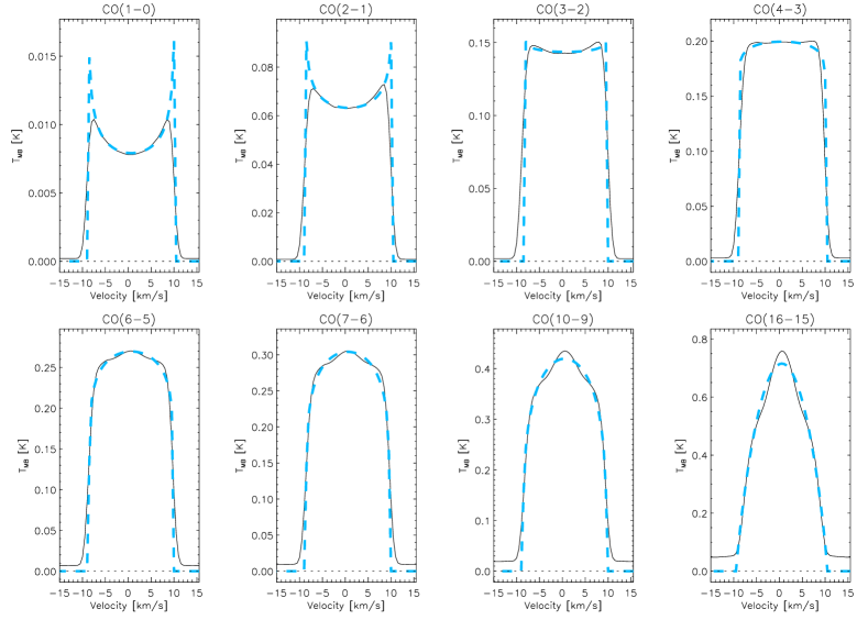
Figure 4: Line profile predictions for $T_{\star}$ = 2000 K, $L_{\star}$ = 3000 $L_{\odot}$, $d$ = 300 pc, $f_{\mathrm{H,CO}}$  = $1\times 10^{-4}$, ¹²C/¹³C = 10, $R_{\rm inner}$ = 3 $R_{\star}$, $\dot{M}$ = $1\times 10^{-7}$ $M_{\odot}$ yr^-1, $v_{\infty}$  = 10 km s^-1 for a beam width of 10^′′. The soft-parabola fit is plotted in dashed grey/light blue lines. For the high-$J$ excitation lines one can see both the stellar and dust continuum and the acceleration zone (the narrow peaks around the line centres).

3 Radiative transfer analysis

Physical information on the envelope structure of evolved stars can be extracted from the observed line fluxes using a non-local thermodynamic equilibrium (non-LTE) radiative transfer code (see Sect. 3.1 for a short description). The availability of a large $\@element[12]{\mathrm{CO}}$ and $\@element[13]{\mathrm{CO}}$ line flux data base, as presented in Sect. 2.3, offers interesting possibilities for statistical analyses. However, this large database also forces us to construct simplified analytical expressions relating the mass-loss rate and the observed integrated CO-line intensities to deduce the mass-loss history of each target. We therefore derived new mass-loss rate formulae based on a grid computation. Similar formalisms that have been presented in the literature are summarised in Sect. 3.2. The grid construction and the resulting analytical expressions are discussed in Sect. 3.3 and 3.4. A discussion on the quality of the formalism can be found in Sect. 3.5.

3.1 Radiative transfer model

The structure of circumstellar envelopes is thought to be quite complex, due to the possible presence of shocks, bipolar outflows, or episodic mass-loss events. The complex heating and cooling processes due to excitation of molecules, and the unknown grain-size distributions contribute to the complexity of the envelopes. The often taken approach to model these envelope structures is therefore to choose a simplified approach with reasonable assumptions. We use the non-LTE radiative code GASTRoNOoM, which was presented and discussed by Decin et al. (2006, 2007, 2008Natureexlaba) and benchmarked according to the method described by van Zadelhoff et al. (2002), considering a simple 2-level molecule (their cases 1a and 1b). The CSE is assumed to be spherically symmetric and formed by a constant mass-loss rate. The code calculates the kinetic temperature and velocity structure in the shell by solving the equations of motion of gas and dust and the energy balance simultaneously Justtanont et al. (1994). Adopting a value for the gas mass-loss rate, the dust-to-gas ratio is adjusted until the required terminal velocity is obtained (Decin et al., 2006). The statistical equilibrium equations and the radiative transfer equation are solved in the co-moving frame using the Approximated Newton-Raphson operator as developed by Schönberg & Hempe (1986). Finally, a ray tracing program uses the computed non-LTE level populations to calculate the line profiles. For a full description of the GASTRoNOoM-code, we refer to Decin et al. (2006).

As described by Decin et al. (2006, 2007, 2008Natureexlaba), a detailed radiative transfer modelling of one target often results in the computation of many ($>10^{5}$) models. Some prior knowledge on the input parameters helps to restrict the extensive parameter space. The main input parameters for this research are the stellar temperature $T_{\star}$, the stellar radius $R_{\star}$, the distance $d$, the CO fractional abundance $f_{\mathrm{H,CO}}=\mathrm{CO/H}$, the $\@element[12]{\mathrm{C}}$/$\@element[13]{\mathrm{C}}$ isotope abundance ratio, the terminal velocity $v_{\infty}$, the mass-loss rate $\dot{M}$, and the dust condensation radius $R_{\mathrm{inner}}$. When each of these eight parameters would only be scanned over five different values, almost 400 000 models should be computed. Performing an in-depth line profile analysis for each target presented in this study is therefore too time-consuming and beyond the scope of this paper. The mass-loss rates of some twenty targets of the current sample will be individually modelled in a forthcoming paper (Lombaert et al., in prep.).

Before describing the grid computation in Sect. 3.3, we give a short overview of mass-loss rate formulae presented in the literature. This overview is for sure not complete, but provides a few often applied formulae, relevant to this study. These formalisms are also compared with the one we present in this paper.

3.2 Comparison with other studies

Several theoretical mass-loss rate formulae based on observed line intensities or fluxes were already presented in the literature. Knapp & Morris (1985) derived a formula to estimate $\dot{M}$ in terms of the CO($J=1-0$) line intensity. Their formula relates the mass-loss rate to an assumed CO abundance and a number of easily determined observables: the main beam temperature $T_{\mathrm{MB,c}}$ at the line centre (in K), the terminal velocity $v_{\infty}$ (in km s^-1), and distance $d$ (in pc). A distinction was made between optically thick and optically thin envelopes. The model for the CO emission assumed a spherically symmetric envelope expanding at constant velocity. The kinetic temperature profile throughout the envelope was assumed in all cases to be that derived by Kwan & Linke (1982) for CW Leo. The statistical equilibrium equations were solved for the lowest 15 rotational levels. Olofsson et al. (1993) transformed the formula of Knapp & Morris (1985) for an optically thick envelope to the slightly more general form

$$\dot{M}_{\mathrm{KM}}=5.7\times 10^{-20}\frac{T_{\mathrm{MB,c}}v_{\infty}^{2}d^{2}\theta_{\rm b}^{2}}{s(J)f_{\mathrm{H,CO}}^{0.85}}\;\mathrm{M}_{\odot}/\mathrm{yr,}$$ (2)

where $\theta_{\rm b}$ is the beamwidth of the instrument (in arcsec) used for the observation of the line under study. The factor $s(J)$ depends on the rotational transition $J\rightarrow J-1$. For the $J=1-0$ transition $s(J)=1$, and for the $J=2-1$ transition $s(J)=0.5$ (see the discussion in Olofsson et al., 1993). In this equation — valid in the optically thick case — the CO envelope size was fixed at $3\times 10^{17}$ cm, appropriate for high-$\dot{M}$ targets. Schöier & Olofsson (2001) compared mass-loss rates derived using their Monte Carlo non-LTE radiative transfer model to those estimated using the formulae of Knapp & Morris (1985). They found that the formula underestimated the mass-loss rates when compared to those obtained from their radiative transfer analysis on average by a factor of about four, and the discrepancies were found to increase for lower mass-loss rate objects (Schöier & Olofsson, 2001, see their Fig. 8). In the case of optically thin envelopes, the exact envelope size matters in estimating $\dot{M}$, so Eq. 2 is indeed of lesser value. A correction for the envelope size (see Neri et al., 1998, and references therein) would decrease the discrepancy found by Schöier & Olofsson (2001). However, considering the simplicity of Eq. 2, the agreement is still remarkably good.

Loup et al. (1993) calculated the envelope size $R_{\mathrm{CO}}$ and the mass-loss rate $\dot{M}_{\mathrm{L}}$ by numerically solving the system of Eqs. 3 and 3.2.

$$\dot{M}_{\mathrm{L}} = \frac{v_{\infty}^{2}d^{2}T_{\mathrm{MB,c}}}{2\times 10^{3}(2f_{\mathrm{H,CO}})^{0.85}}\times F^{-1}(R_{\mathrm{CO}})\;\;\mathrm{M}_{\odot}\,\mathrm{yr}^{-1}$$ (3)

$$\dot{M}_{\mathrm{L}} = 10^{-6}\left(\frac{R_{\mathrm{CO}}}{7.3\times 10^{16}}\right)^{1/0.58}\left(\frac{v_{\infty}}{10}\right)^{1/1.45}$$

$$\quad\times\left(\frac{4\times 10^{-4}}{2f_{\mathrm{H,CO}}}\right)^{1/1.16}\;\;\mathrm{M}_{\odot}\,\mathrm{yr}^{-1}$$

They assumed $f_{\mathrm{H,CO}}$ of $2.5\times 10^{-4}$ for oxygen-rich stars and $5\times 10^{-4}$ for both carbon-rich and S-type stars. The function $F(R_{\mathrm{CO}})$ introduces a correction factor for the envelope size and is normalised to unity for $R_{\mathrm{CO}}=3\times 10^{17}$ cm.

Ramstedt et al. (2008) derived a formula relating the mass-loss rate to the integrated intensity $I_{{\rm CO},J}$ of the $\@element[12]{\mathrm{CO}}$ ($J\rightarrow J-1$) lines, the terminal velocity $v_{\infty}$, the abundance $f_{\mathrm{H,CO}}$, the distance $d$ to the object, and the telescope’s beam size $\theta_{\rm b}$. Using the Monte Carlo radiative transfer code described by Schöier & Olofsson (2001), the estimator was derived from a grid of 60 models varying in $\dot{M}$ (1, 3, 10, 30, and 100 $\times 10^{-7}$ M_⊙  yr^-1), $v_{\infty}$ (5, 10, 15, and 20 km s^-1), and $f_{\mathrm{H,CO}}$ (1, 3, and 10 $\times 10^{-4}$). The distance was taken to be 1000 pc. For each model, the velocity integrated intensities in CO ($J=1-0,\;2-1,\;3-2,\;4-3$) were calculated for a 20 m telescope (with corresponding beam sizes of 33^′′, 16.5^′′, 11^′′, and 8.5^′′). They use the so-called $h$-parameter to describe the free parameters of the dust (Schöier & Olofsson, 2001):

$$h=\left(\frac{\Psi}{0.01}\right)\left(\frac{2.0\ \mathrm{g\ cm^{-3}}}{\rho_{\mathrm{d}}}\right)\left(\frac{0.05\ \mu\mathrm{m}}{a_{\mathrm{d}}}\right),$$ (5)

where $\Psi$ is the dust-to-gas mass ratio, and $\mathrm{\rho_{d}}$ and $a_{\mathrm{d}}$ are the average density and the radius of an individual dust grain, respectively. The value of $h$ was assumed to be 0.2 for $\dot{M}$ in the range up to $3\times 10^{-7}$ M_⊙  yr^-1, 0.5 for $1-3\times 10^{-6}$M_⊙  yr^-1, and 1.5 for $10^{-5}$ M_⊙  yr^-1. The stellar temperature $T_{\star}$, stellar radius $R_{\star}$ or inner dust condensation radius $R_{\mathrm{inner}}$ were not specified. An estimate for the mass-loss rate was determined from a minimisation procedure applied to Eq. 6:

$$\dot{M}_{\mathrm{R}}=s_{J}(I_{\mathrm{CO},J}\theta_{\mathrm{b}}^{2}d^{2}/10^{6})^{a_{J}}v_{\infty}^{b_{J}}f_{\mathrm{H,CO}}^{-c_{J}}\mathrm{M}_{\odot}\,\mathrm{yr}^{-1},$$ (6)

with $I_{{\rm CO},J}$ in K km s^-1, $v_{\infty}$ in km s^-1, $d$ in pc, and $\theta_{\rm b}$ in arcsec. A comparison between their input mass-loss rates and the values found from Eq. 6 was not shown, nor were estimates of the uncertainties on the derived $\dot{M}$-values provided. The comparison between mass-loss rates derived using Eq. 6 and mass-loss rates derived using their Monte Carlo code for a sample of C-, M- and S-stars shows quite a good agreement. Close inspection, however, reveals that for low-$J$ transitions ($J=1-0,\,2-1$) Eq. 6 tends to underestimate the mass-loss rate for $\dot{M}\lesssim 10^{-6}$ M_⊙  yr^-1 and to overestimate it for $\dot{M}\gtrsim 10^{-5}$ M_⊙  yr^-1 (see Fig A.1. in Ramstedt et al., 2008).

Since (1) our data set holds observations up to the high excitation $J=6-5$ and $J=7-6$ rotational line transitions of CO, and we want (2) to include the shape of the line profiles, represented by parameter $\beta$, in the estimates of $\dot{M}$, and (3) to extend the computations to higher mass-loss rate values ($\dot{M}$$>1\times 10^{-5}$ $M_{\odot}$ yr^-1), we elaborated on the studies discussed above by performing a grid computation covering more than 15 000 models.

Table 2: Values for the input parameters used in the grid computations.

Param.	Grid values	Param.	Grid values
$T_{\star}$	2000, 2500, 3000 K	$R_{\rm inner}$	3, 10, 30 $R_{\star}$
$L_{\star}$	3000, 10 000, 30 000 L⊙	12C/13C	10, 30, 100
$d$	300,  1000,  3000 pc	$\dot{M}$	1, 3, 10, 30,
$v_{\infty}$	10, 15, 20 km s-1		100, 300, 1 000
$f_{\mathrm{H,CO}}$	1, 3, 5$\times 10^{-4}$		$\times 10^{-7}$M⊙  yr-1
$\theta$	10, 20, 30′′

3.3 Description of the grid

To study the influence of different stellar and envelope parameters — like stellar temperature, stellar radius (or stellar luminosity) and dust condensation radius — on the CO line intensities, the input parameters were varied to cover the relevant parameter space for evolved low-mass targets (see Table 2). The values for the $f_{\mathrm{H,CO}}$ were chosen to be $1\times 10^{-4}$ for O-rich stars (Kahane & Jura, 1994), $3\times 10^{-4}$ for S-type stars (Ramstedt et al., 2006), and $5\times 10^{-4}$ for C-rich stars (Zuckerman & Dyck, 1986). All computations were performed for a 15 m class telescope, with beam sizes of 10^′′, 20^′′ and 30^′′ as grid input values. This grid spans 15 309 star models, for which each rotational line intensity was computed for three values of the beamwidth.

As was done for the observational line profiles, the theoretical line profiles were fitted with a soft parabola. In the case of the theoretical line profiles, however, an extra offset $T_{0}^{g}$ should be added to the equation, resulting in

$$T^{g}(v) = T^{g}_{\mathrm{MB,c}}\left[1-\left(\frac{v^{g}-v^{g}_{\mathrm{LSR}}}{v^{g}_{\infty}}\right)^{2}\right]^{\beta/2}+T_{0}^{g}$$

$$\qquad\qquad\qquad\qquad\qquad{\rm for\ }|v^{g}-v^{g}_{\mathrm{LSR}}|\leq v^{g}_{\infty}$$

$$= T_{0}^{g}\ \ \qquad\qquad\qquad\qquad\,{\rm for\ }|v^{g}-v^{g}_{\mathrm{LSR}}|>v^{g}_{\infty}$$

where $T$ is the line intensity in main-beam temperature. The superscript ’$g$’ designates that we are dealing with theoretical profiles that were computed using the GASTRoNOoM-code. The reason for the offset is that, in case of optically thin envelopes, one still detects the almost unattenuated stellar continuum (see Fig. 4). This offset parameter is not present in Eq. 2.3.1 that was used to fit the data. During the data-reduction process, the offset is removed from the spectra when baselines are subtracted, since the observer does not know if and how much stellar light penetrates the envelope. When confronting observational data with theoretical integrated line intensities, one therefore has to compare $I^{g}-2v_{\infty}T^{g}_{0}$ to $I$, where $I$ is the integrated line intensity $\int T(v)dv$ in K km s^-1. The quantity $I^{g}-2v_{\infty}T^{g}_{0}$ will from now on be referred to as $I^{g,cc}$, with the superscript ’$cc$’ denoting the continuum correction. Optically thin lines allow one to trace the wind acceleration zone of which the emission is visible as a superimposed small peak around the line centre (see Fig. 4).

The soft-parabola fit is not ideal to reproduce optically thin resolved emission lines (see upper panels of Fig. 4). The $\beta$-value was determined in a way that the soft parabola should yield a good representation of the line depression. The integrated intensity of the fit was not required to match the integrated intensity of the GASTRoNOoM-predictions. This method provides information about the degree to which the line profiles are resolved by the telescope beam.

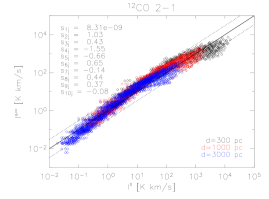
Figure 5: The continuum corrected integrated intensities $I^{g,cc}$ predicted with GASTRoNOoM are compared to the values $I^{\mathrm{D}}$ calculated with Eq. 3.4. Values for the exponents $s_{i,J}$ in Eq. 3.4 are specified in the upper left corner. The full line represents equality of $I^{g,cc}$ and $I^{\mathrm{D}}$, the dotted lines show a factor 3 difference w.r.t. this relation. For all three distance values assumed in the model grid, the estimates are plotted in a different color: black for $d=300$ pc, red for $d=1000$ pc, and blue for $d=3000$ pc. See Sect. 3.4 for further details.

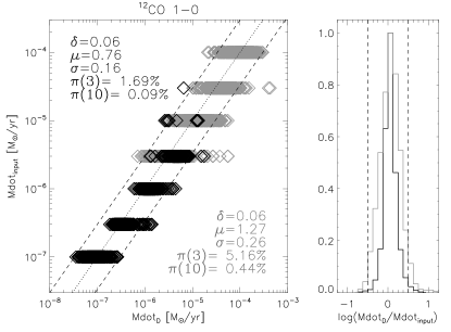
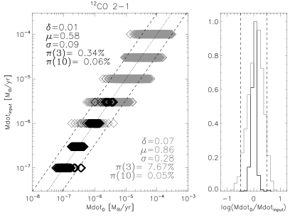
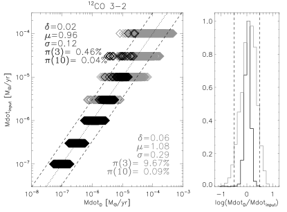
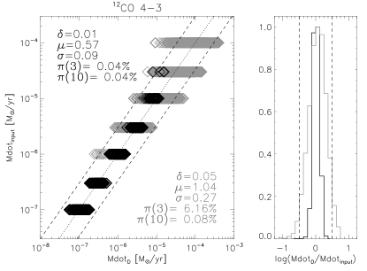
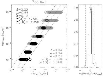
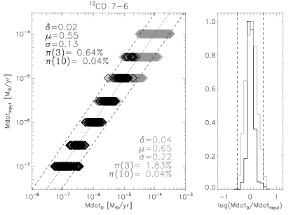
Figure 6: Comparison between the input value $\dot{M}_{\mathrm{input}}$ and $\dot{M}_{\mathrm{D}}$ resulting from using Eq. 9 for different rotational CO line transitions. Estimates for the non-saturated regime are plotted in black, for the saturated regime in grey. The dotted line represents equality of the input and estimated mass-loss rates, the dashed lines show a factor 3 difference w.r.t. this relation. The listed $\delta$, $\sigma$, and $\mu$ are the mean, the standard deviations, and the maximum absolute values of $\log(\dot{M}_{\mathrm{D}}/\dot{M}_{\mathrm{input}})$, respectively. $\pi(3)$ and $\pi(10)$ show the percentage of grid models that produce values of $\dot{M}_{\mathrm{D}}$ deviating more than a factor 3, resp. 10, from $\dot{M}_{\mathrm{input}}$. The histogram on the right of each panel shows the peak-normalised distribution of $\log(\dot{M}_{\mathrm{D}}/\dot{M}_{\mathrm{input}})$. The vertical dashed lines in these histograms again show a factor three difference between $\dot{M}_{\mathrm{D}}$ and $\dot{M}_{\mathrm{input}}$. The black and grey histograms represent estimates for the non-saturated, and saturated regimes, respectively.

Table 3: Values for the exponents $s_{i,J}$ in Eq. 9 for each $\@element[12]{\mathrm{CO}}$ ($J\rightarrow J-1$) transition. The boundary values for saturation (see text for further details) are given in the third column. The $s_{i,J}$ are calibrated such that the mass-loss rate $\dot{M}_{\mathrm{D}}$ is in units of M_⊙  yr^-1. Standard deviations $\sigma$, maximum absolute values $\mu$, and mean values $\delta$ of $\log(\hbox{$\dot{M}$}_{\mathrm{D}}/\dot{M}_{\mathrm{input}})$ are given in the last three columns.

Regime	Transition	$I_{\mathrm{MB}}\times d^{2}$	$s_{1,J}$	$s_{2,J}$	$s_{3,J}$	$s_{4,J}$	$s_{5,J}$	$s_{6,J}$	$s_{7,J}$	$s_{8,J}$	$s_{9,J}$	$s_{10,J}$	$\sigma$	$\mu$	$\delta$
		[K km s-1 $\times$ pc2]
unsat.	$1-0$	$<1\times 10^{7}$	$9.73\times 10^{-16}$	1.25	0.31	-1.78	-1.29	1.03	0.33	0.10	0.21	-0.01	0.16	0.76	0.06
sat.	$1-0$	$\geq 1\times 10^{7}$	$9.16\times 10^{-9}$	0.78	0.50	-1.22	-0.34	0.44	-0.66	0.28	0.37	-0.03	0.26	1.27	0.06
unsat.	$2-1$	$<2\times 10^{7}$	$1.00\times 10^{-15}$	1.26	0.05	-1.96	-1.26	0.79	0.05	0.24	0.10	0.07	0.09	0.58	0.01
sat.	$2-1$	$\geq 2\times 10^{7}$	$9.04\times 10^{-10}$	0.75	0.43	-1.47	-0.08	0.39	-1.00	0.35	0.41	-0.00	0.28	0.86	0.07
unsat.	$3-2$	$<9\times 10^{7}$	$9.93\times 10^{-14}$	1.14	0.13	-1.92	-1.39	0.78	-0.25	0.40	0.29	-0.11	0.12	0.96	0.02
sat.	$3-2$	$\geq 9\times 10^{7}$	$9.34\times 10^{-10}$	0.61	0.31	-1.67	-0.00	0.36	-1.00	0.37	0.43	0.01	0.29	1.08	0.06
unsat.	$4-3$	$<9\times 10^{7}$	$9.69\times 10^{-15}$	1.17	0.04	-1.98	-1.26	0.79	-0.38	0.39	0.32	0.02	0.09	0.57	0.01
sat.	$4-3$	$\geq 9\times 10^{7}$	$9.30\times 10^{-10}$	0.63	0.25	-1.77	-0.06	0.38	-1.00	0.42	0.45	0.03	0.27	1.04	0.05
unsat.	$6-5$	$<1\times 10^{8}$	$9.43\times 10^{-14}$	1.12	0.01	-1.99	-1.19	0.75	-0.48	0.46	0.42	-0.04	0.12	0.66	0.02
sat.	$6-5$	$\geq 1\times 10^{8}$	$9.52\times 10^{-10}$	0.69	0.15	-1.86	-0.22	0.49	-1.00	0.52	0.46	-0.11	0.23	0.94	0.04
unsat.	$7-6$	$<2\times 10^{8}$	$9.44\times 10^{-12}$	1.09	0.01	-1.99	-1.06	0.77	-0.42	0.57	0.52	-0.02	0.13	0.55	0.02
sat.	$7-6$	$\geq 2\times 10^{8}$	$9.44\times 10^{-10}$	0.64	0.12	-1.87	-0.21	0.47	-1.00	0.51	0.47	-0.15	0.22	0.65	0.04
unsat.	$10-9$	$<2\times 10^{8}$	$9.73\times 10^{-10}$	0.98	0.00	-2.00	-0.72	0.68	-0.47	0.63	0.60	0.01	0.13	0.45	0.02
sat.	$10-9$	$\geq 2\times 10^{8}$	$9.41\times 10^{-10}$	0.58	0.03	-1.93	-0.08	0.49	-1.00	0.51	0.47	-0.15	0.24	0.67	0.05
unsat.	$16-15$	$<2\times 10^{8}$	$9.84\times 10^{-10}$	0.87	0.01	-1.98	-0.57	0.61	-0.85	0.65	0.61	0.02	0.16	0.52	0.03
sat.	$16-15$	$\geq 2\times 10^{8}$	$9.20\times 10^{-10}$	0.48	0.02	-1.92	0.00	0.47	-1.00	0.46	0.43	-0.09	0.31	0.92	0.10

The values in Table 3 show that the dependence of the integrated intensity on the distance is strongest. For the unsaturated regime, the integrated intensity is quite sensitive on the terminal velocity and mass-loss rate, while this dependence is, as expected, much lower in the saturated regime. The intensity is moderately dependent on $\beta$, the stellar temperature, stellar radius, and dust condensation radius.

3.4 Grid results

To estimate the minimisation function to the integrated intensities, the dependence of the integrated intensity $I^{g}$ on the different input parameters was inspected, and a power-law relation between the integrated intensity and all parameters was assumed. To estimate the outcome variable $I^{g,cc}$ we therefore have minimised the function

$$I^{\mathrm{D}} = \frac{1}{s_{1,J}}\dot{M}^{s_{2,J}}\theta_{\rm b}^{s_{3,J}}d^{s_{4,J}}v_{\infty}^{s_{5,J}}f_{\mathrm{H,CO}}^{s_{6,J}}$$

$$\qquad\times\;T_{\star}^{s_{7,J}}R_{\star}^{s_{8,J}}R_{\mathrm{inner}}^{s_{9,J}}\beta^{s_{10,J}}.$$

The minimisation was carried out for each $\@element[12]{\mathrm{CO}}$ line transition, using the generalized reduced gradient method (Lasdon et al., 1978). The correlation between the GASTRoNOoM output variable $I^{g,cc}$ and the integrated intensity $I^{\mathrm{D}}$ derived from Eq. 3.4 is not bad, but a clear saturation effect is visible for all transitions when $I^{g,cc}$ exceeds a certain boundary value (see Fig. 5). These boundary values are higher for higher $J$. A higher mass-loss rate not only leads to an increase of the cooling of the circumstellar gas, but also to a decrease in drift velocity between the dust and the gas (Decin et al., 2006). This leads to a weaker dependence of the integrated intensity of the CO lines on $\dot{M}$, visible as saturation. Not accounting for this saturation effect typically leads to underestimating $\dot{M}$ by a factor of $3-10$ for $\dot{M}\geq 3\times 10^{-5}$ M_⊙  yr^-1.
Moreover, it is visible from Fig. 5 that the boundary values for saturation are distance dependent, with lower boundary values for larger distances. This dependence was removed by minimising Eq. 3.4 again, but with both the left-hand and the right-hand side multiplied with a factor $d^{2}$. The coefficients $s_{i,J}$ for $J=1-0,\;2-1,\;3-2,\;4-3,\;6-5,\;7-6,\;10-9,\;16-15$ and the boundary values of $I_{\mathrm{MB}}\times d^{2}$ for saturation are listed in Table 3.

Replacing $I^{\mathrm{D}}$ in Eq. 3.4 with the observed integrated line intensity $I_{\mathrm{MB}}$ yields an estimate for the mass-loss rate, $\dot{M}_{\mathrm{D}}$, provided that the other parameters are known:

$$\dot{M}_{\mathrm{D}}=\left[\frac{s_{1,J}\times I_{\mathrm{MB}}}{\theta_{\rm b}^{s_{3,J}}d^{s_{4,J}}v_{\infty}^{s_{5,J}}f_{\mathrm{H,CO}}^{s_{6,J}}T_{\star}^{s_{7,J}}R_{\star}^{s_{8,J}}R_{\mathrm{inner}}^{s_{9,J}}\beta^{s_{10,J}}}\right]^{\frac{1}{s_{2,J}}}.$$ (9)

In Fig. 6 we show a comparison between the mass-loss rate $\dot{M}_{\mathrm{input}}$ used as input for the grid models, and the mass-loss rate $\hbox{$\dot{M}$}_{\mathrm{D}}$, calculated from the CO line intensities that result from the models, using Eq. 9. In Table 3 and Fig. 6 we listed the mean values $\delta$, standard deviations $\sigma$, and maximum absolute values $\mu$ of the quantity $\log(\hbox{$\dot{M}$}_{\mathrm{D}}/\dot{M}_{\mathrm{input}})$. All listed $\delta$-values are positive, meaning that on average we slightly overestimate the input-mass-loss rate. This is however limited to overestimates of a few percents only, except for the cases of $1-0$ (15 %, $\delta$=0.06), and $2-1$ in the saturated regime (17 %, $\delta$=0.07). These deviations are still well within the standard deviation $\sigma$ and therefore not significant. In the panels of Fig. 6 we also mention the quantities $\pi(3)$ and $\pi(10)$. These are the percentages of models in the grid that result in a value of $\hbox{$\dot{M}$}_{\mathrm{D}}$ that deviates by more than a factor 3, resp. 10, from the input mass-loss rate. The $\sigma$-values indicate uncertainties of a factor $\sim$1.3 for the unsaturated regime, and a factor $\sim$1.9 for the saturated regime when comparing $\hbox{$\dot{M}$}_{\mathrm{D}}$ to $\dot{M}_{\mathrm{input}}$. When applying Eq. 9 to data, the error bars on the measured parameters, e.g. $T_{\star}$, add to these uncertainties, increasing the typical uncertainty to a factor of three.

The spread on the estimates reflects the interplay between the different stellar parameters and the line intensities, and the large parameter space covered by the grid. In the saturated regime the spread is somewhat larger than in the unsaturated regime, with standard deviations $\sigma$ ranging up to 0.16 and 0.31 in the unsaturated and saturated regimes, respectively. These values are still rather low, and are also reflected in the values of $\pi(3)$ and $\pi(10)$ that do not exceed $10\,\%$ and $0.45\,\%$ in the saturated regime, clearly showing the very small number of outliers present in our results. We point out that we found no obvious relations between the (few) grid points showing the larger values of $|\log(\hbox{$\dot{M}$}_{\mathrm{D}}/\dot{M}_{\mathrm{input}})|$. Therefore, we do not attach larger intrinsic uncertainties to specific input parameters. The quantities $\sigma,\,\mu,\,\delta,\,\pi$ indicate a high accuracy of the estimator for the complete range of mass-loss rates included in the grid (Table 2).

3.5 Discussion on the derived mass-loss rate formulae

3.5.1 Varying the number of free parameters

As was done in other studies (e.g. Ramstedt et al., 2008), one can lower the number of free parameters in Eq. 3.4. This is illustrated in Fig. 7 for the $J=2-1$ transition. We show the estimates in two cases, omitting the dependence of the integrated intensity on $\beta$ and $R_{\mathrm{inner}}$ (left panel) and on $\beta$, $R_{\mathrm{inner}}$, $T_{\star}$, and $R_{\star}$ (right panel). Mainly for the mass-loss rates exceeding $10^{-5}$ M_⊙  yr^-1, the estimates exhibit larger uncertainties. An overview of the values for the standard deviations $\sigma$, and maximum absolute values $\mu$ of $\log(\dot{M}_{\mathrm{D}}/\hbox{$\dot{M}$}_{\mathrm{input}})$ is given in Table 4 for the different cases. Both $\mu$ and $\sigma$ increase significantly when lowering the number of parameters. This implies that it is better to include a well-founded estimate for some parameter, like $\beta$ or $R_{\mathrm{inner}}$, than to omit it from Eq. 3.4.

Table 4: Standard deviations $\sigma$ and maximum deviations $\mu$ of $\log(\dot{M}_{\mathrm{D}}/\dot{M}_{\mathrm{input}})$ for the different numbers of parameters included in the formalism. Values for both the unsaturated and saturated regimes for $\@element[12]{\mathrm{CO}}$ ($J=2-1$) are shown.

$\@element[12]{\mathrm{CO}}$ ($J=2-1$)	$\sigma$		$\mu$
	unsat.	sat.	unsat.	sat.
all parameters	0.09	0.28	0.58	0.86
no $\beta$, $R_{\mathrm{inner}}$	0.10	0.42	0.62	1.13
no $\beta$, $R_{\mathrm{inner}}$, $T_{\star}$,$R_{\star}$	0.19	0.46	0.78	1.32

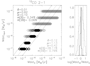
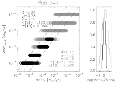
Figure 7: Comparison between the input value $\dot{M}_{\mathrm{input}}$ (ordinate) and $\dot{M}_{\mathrm{D}}$ resulting from using a formula analogous to Eq. 9 (abscissa) for different rotational CO line transitions, but omitting the dependence of the mass-loss rate on $R_{\rm inner}$ and $\beta$ (left panel), and on $R_{\rm inner}$, $\beta$, $T_{\star}$ , and $R_{\star}$ (right panel). Estimates for the non-saturated regime are plotted in black, for the saturated regime in grey. $\delta,\,\sigma,\,\mu,\,\pi(3)$ and $\pi(10)$ are as in Fig.6. The dotted line represents equality of the input and estimated mass-loss rates, the dashed lines show a factor 3 difference w.r.t. this relation. The histogram on the right of each panel shows the peak-normalised distribution of $\log(\dot{M}_{\mathrm{D}}/\dot{M}_{\mathrm{input}})$. The vertical dashed lines in these histograms again show a factor three difference between $\dot{M}_{\mathrm{D}}$ and $\dot{M}_{\mathrm{input}}$.

3.5.2 Sensitivity analysis

To further assess the quality of our estimator, we focus on the influence of (1) input parameters for Eq. 9, such as effective temperature, luminosity, dust condensation radius, photospheric CO abundance, and distance, (2) the envelope’s outer radius, and (3) the gas kinetic temperature.

Input parameters:

We tested the influence of $d$, $T_{\star}$, $L_{\star}$ ($R_{\star}$), $f_{\mathrm{H,CO}}$ and $R_{\mathrm{inner}}$ on the $\dot{M}$-estimates for $J=1-0,\,2-1,\,3-2,\,4-3,\,6-5,\,7-6$. We assumed a standard stellar model with $\dot{M}_{\mathrm{input}}$ $=10^{-7}$ M_⊙  yr^-1, $T_{\star}$ $=2000$ K, $R_{\star}$ $=3.14\times 10^{13}$ cm, $R_{\mathrm{inner}}$ $=3$ $R_{\star}$, $f_{\mathrm{H,CO}}$ $=10^{-4}$, $d=300$ pc, and a fixed beamwidth $\theta_{\mathrm{b}}=10$ ^′′. The integrated intensities $I_{\mathrm{MB}}$ are those calculated with the GASTRoNOoM-code for this model. In Fig. 8 we show the influence of the different parameters on the $\dot{M}$-estimates by varying $d$, $f_{\mathrm{H,CO}}$, $T_{\star}$, $L_{\star}$ and $R_{\mathrm{inner}}$ one by one while keeping all others constant at the model values. We point out that a slight gradient is present in the $\dot{M}$-estimates for the standard model, i.e. for higher $J$ we seem to estimate somewhat lower values of $\dot{M}$. The deviations and the spread of the estimates are, however, well within a factor three from the input mass-loss rate. Since the latter is used as a criterion to decide upon constancy of $\dot{M}$, we can state that the estimator can very well reproduce the input-$\dot{M}$.

As expected, the distance has the strongest influence on the estimated $\dot{M}$-values, with a similar increase or decrease in mass-loss rate for all transitions. Altering $f_{\mathrm{H,CO}}$ has a pure scaling effect on the estimates, with a lower $\dot{M}$ for a higher $f_{\mathrm{H,CO}}$. Changing $T_{\star}$, $L_{\star}$, or $R_{\mathrm{inner}}$ leads to the largest differences for the higher-$J$ transitions, since changing these parameters affects the layers closest to the star more strongly than it does the more outward layers. This effect is reflected in the larger absolute values of exponents $s_{7,J},\,s_{8,J}$ and $s_{9,J}$ in Eq. 9, and by the fact that the mentioned gradient is slightly shallower or steeper when considering other values for $T_{\star}$, $L_{\star}$, or $R_{\mathrm{inner}}$. This implies that the estimates based on the higher-$J$ transitions suffer from larger uncertainties and that more value can be attached to the estimates based on the lower-$J$ transitions.

Inspecting the different panels in Fig. 8, we find no indications for changes in the $\dot{M}$-estimates with an opposite character for the different transitions, in the sense that, e.g., the estimates for some $J$ would go lower, while those for other transitions go higher. For a constant mass-loss rate we will therefore only see a gradient (if any) and not a random distribution of the estimates. This implies that a faulty parameter assumption will only lead to a general shift of the estimates and is unlikely to change the interpretation of possible variability or constancy of the mass-loss rate.

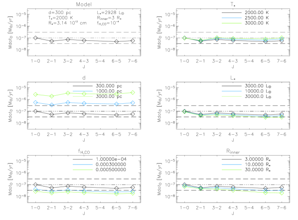
Figure 8: Sensitivity check of the used formalism for five parameters: $d$, $f_{\mathrm{H,CO}}$, $T_{\star}$, $L_{\star}$ ($R_{\star}$), and $R_{\mathrm{inner}}$. The upper left panel gives the estimates based on the input parameters of the model and the output values of the integrated intensities $I^{\mathrm{g,cc}}$. The grid values for the different parameters and the colour coding are specified in the legend of every panel. The dash-dotted line in all panels marks the model’s input-$\dot{M}$, $10^{-7}$ M_⊙  yr^-1, the dashed lines mark a factor three difference w.r.t. this value.

Outer envelope radius:

The influence of the outer radius of the CSE, $R_{\mathrm{outer}}$, can not be tested in the same way since it is not an input parameter in Eq. 9. This variable has therefore no direct influence on the estimates. It did however influence the derivation of the coefficients $s_{i,J}$, since the geometrical extent of the envelope affects the integrated intensities and the shapes of the emission lines. The transition most sensitive to changes in $R_{\mathrm{outer}}$ is $J=1-0$, implying that it is a safer choice to use $\dot{M}$-estimates based on the $J=2-1$ transition.

Clumping of CSE material causes a larger $R_{\mathrm{outer}}$ than a smooth mass outflow because of shielding properties of the clumps. This implies that higher integrated intensities can be reached with the same mass-loss rate. Therefore, if clumping is present, we could be overestimating the mass-loss rate. This will again be most strongly reflected in the $J=1-0$ estimates.

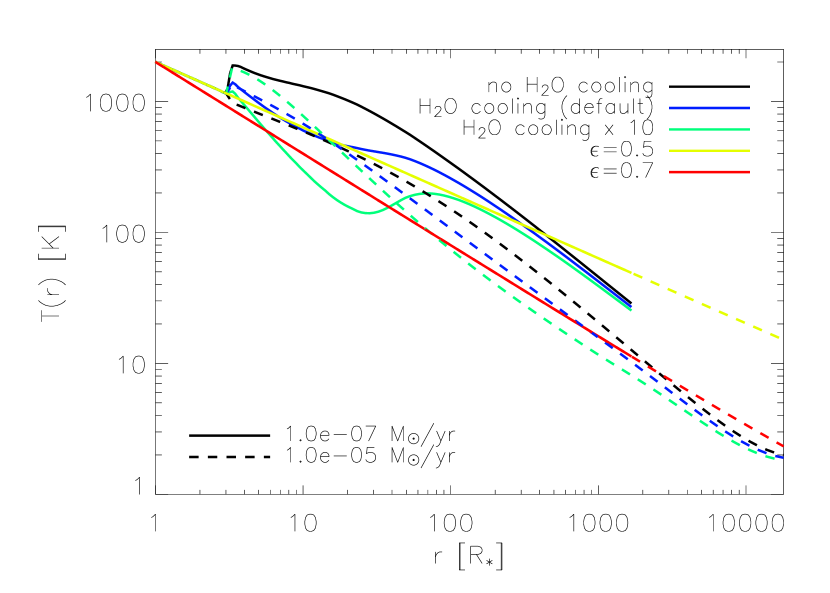
(a) Gas kinetic temperature $T$ versus radius $r$ for $\dot{M}$ =$10^{-7}$ M_⊙  yr^-1 (full line), and $10^{-5}$ M_⊙  yr^-1 (dotted line).

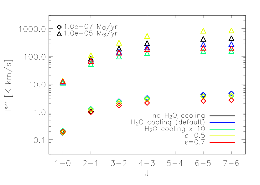
(b) Integrated intensities $I^{g,cc}$ for transitions $J=1-0$ up to $J=7-6$.

Figure 9: Gas kinetic temperatures (a) and integrated intensities (b) for different $\dot{M}_{\mathrm{input}}$-values and different cooling mechanisms. The colour coding in both panels is as follows: black was used for omission of H₂O-cooling, blue for inclusion of H₂O-cooling, green for inclusion of H₂O-cooling ten times stronger than by default, yellow for a temperature power law, as in Eq. 10, with $\epsilon=0.5$, and red for $\epsilon=0.7$. In the lower panel, the different values of the input-mass-loss rate are indicated with diamonds and triangles for $\dot{M}$ =$10^{-7}$ M_⊙  yr^-1 and $10^{-5}$ M_⊙  yr^-1, respectively. See discussion in Sect. 3.5.2.

Gas kinetic temperature:

In Fig. 9 we compare gas kinetic temperatures $T$, which have been consistently computed with the GASTRoNOoM-code, and integrated intensities $I^{g,cc}$ of transitions $J=1-0$ up to $J=7-6$ for two different values of $\dot{M}_{\mathrm{input}}$ ($10^{-7}$ M_⊙  yr^-1 and $10^{-5}$ M_⊙  yr^-1) and five different effects in cooling. All other model parameters are the same as those mentioned above for the standard model. The default cooling scheme, which was used to derive the formalism presented in this paper, includes among others cooling due to rotational excitation of H₂O. The cooling schemes we considered (1) ignore the H₂O-cooling, (2) include H₂O-cooling (default), (3) include H₂O-cooling ten times stronger than assumed by default, (4) assume a power law for the gas kinetic temperature

$$T(r)=\hbox{$T_{\star}$}\left(\hbox{$R_{\star}$}/r\right)^{\epsilon}$$ (10)

with $\epsilon=0.5$, and (5) assume a power law with $\epsilon=0.7$.

We point out that, except for the cases in which a power law was used to describe $T(r)$, the temperature can increase or decrease with increasing radius $r$, i.e., instead of cooling there can be heating of the envelope; see Fig. 9.

We focus on the H₂O rotational cooling since this part of the cooling is still subject to large uncertainties. In GASTRoNOoM, H₂O is modelled as a three-level system, which is a gross simplification of the actual structure of the molecule. The rotational rate coefficients used here are based on the results of Green et al. (1993), as are those of Neufeld & Kaufman (1993). Faure & Josselin (2008) recently calculated new rotational rates and compared them to those of Neufeld & Kaufman (1993), finding higher cooling rates for temperatures $\lesssim 1500$ K and lower cooling rates for temperatures $\gtrsim 1500$ K. They also found that the rotational rate coefficients can be uncertain by factors of a few up to an order of magnitude, which is reflected in the uncertainties on the cooling rates.

The contribution of H₂O-cooling is most important in the inner wind regions, since farther out in the envelope CO-rotational cooling and especially cooling due to adiabatic expansion dominate. This implies that the gas kinetic temperature in the inner wind regions is more uncertain than in the rest of the envelope.

As is visible in Fig. 9(b), $I^{g,cc}$ decreases for increasing H₂O-cooling. Again, this effect is more explicit for higher $J$. Overestimating the H₂O-cooling therefore leads to an underestimate of the mass-loss rate, considering the relation between the integrated intensities and the $\dot{M}$-estimates.

Since the excitation regions of the higher-$J$ transitions are partly situated in the inner wind regions, the integrated intensities of these transitions will be subject to larger uncertainties than those of the low-$J$ transitions $J=1-0$ and $2-1$. This different degree of influence on the integrated intensities for the different $J$-values is very clear in Fig. 9(b), where the spread on the integrated intensities of the transitions $J\rightarrow J-1$ increases for higher $J$. A second implication is that the mentioned gradient of (slightly) lower $\dot{M}$ for higher $J$-values is possibly linked to the uncertainties on the H₂O-cooling in the inner regions. If this is indeed the case, then the H₂O-cooling rates used in our models are overestimates of the actual rates.

Considering the current models, the uncertainties on the intensities of higher-$J$ transitions (as discussed above), and taking into account that the intensities of the $J=1-0$ transition can be affected by e.g. masering and clumping, we put forward that the $J=2-1$ transition is likely the most reliable transition to use in estimating mass-loss rates.

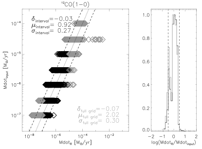
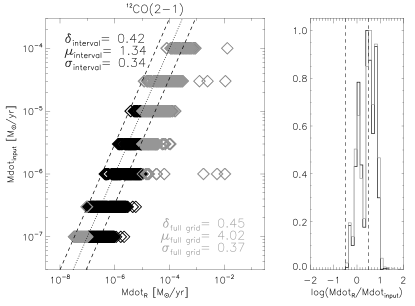
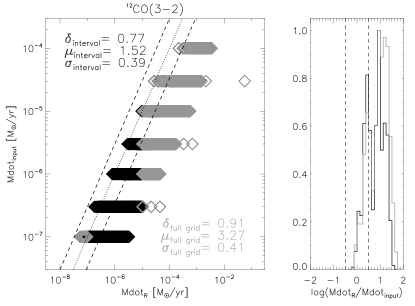
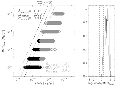
Figure 10: $\dot{M}_{\mathrm{input}}$ versus $\dot{M}_{\mathrm{R}}$ calculated from the grid also used to construct Fig. 6 and Eq. 6. The dotted line indicates where the quantities are equal, the dashed lines show a factor three difference w.r.t. this relation. The listed $\delta,\,\mu$, and $\sigma$ are, respectively, the mean values, the standard deviations, and the maximum absolute values of $\log(\dot{M}_{\mathrm{R}}/\dot{M}_{\mathrm{input}})$. We specify these quantities for the full grid (plotted in grey), and for the grid points inside the interval $[10^{-7};\,10^{-5}]$ M_⊙  yr^-1 (plotted in black). The histogram in each panel shows the peak-normalised distribution of $\log(\dot{M}_{\mathrm{R}}/\dot{M}_{\mathrm{input}})$.

3.5.3 Comparison to Ramstedt et al. (2008)

In benchmarking our formalism against mass-loss rate estimators presented in the literature, we focus on the one derived by Ramstedt et al. (2008). A direct comparison to the estimators of Knapp & Morris (1985) or Loup et al. (1993) is not possible, since these have the main-beam temperature at the line centre, $T_{\mathrm{MB,c}}$, as a fundamental parameter, while we consider the integrated intensity $I_{\mathrm{MB}}$ and the shape of the lines.

In Fig. 10 we show the mass-loss rate estimates derived for transitions $J=1-0,\;2-1,\;3-2$ and $4-3$ via Eq. 6, using the same parameter grid as was used to derive the formalism presented in this paper. Ramstedt et al. (2008) mention that their estimator $\dot{M}_{\mathrm{R}}$ is only valid for mass-loss rates between $10^{-7}$ and $10^{-5}$ M_⊙  yr^-1, so we marked those outside this interval in grey, for the sake of the clarity. Ramstedt et al. (2008) also note the requirement of unresolved envelopes to use their estimator to high accuracy, and we therefore eliminated the grid points that result in resolved envelopes by determining the CO-photodissociation radius, $R_{\mathrm{CO}}$, and subsequently the outer radius, $R_{\mathrm{outer}}$, of the envelope according to Stanek et al. (1995) and Schöier & Olofsson (2001):

$$R_{\mathrm{CO}} = 5.4\times 10^{16}\left(\frac{\hbox{$\dot{M}$}}{10^{-6}}\right)^{0.65}$$ (11)

$$\times\left(\frac{15}{\hbox{$v_{\infty}$}}\times\frac{f_{\mathrm{H,CO}}(\hbox{$R_{\star}$})}{4\times 10^{-4}}\right)^{0.55}$$

$$+7.5\times 10^{15}\left(\frac{\hbox{$v_{\infty}$}}{15}\right)\mathrm{\,cm}$$

$$\alpha = 2.79\times\left(\frac{\hbox{$\dot{M}$}}{10^{-6}}\times\frac{15}{\hbox{$v_{\infty}$}}\right)^{0.09}$$ (12)

$$f_{\mathrm{H,CO}}(r) = f_{\mathrm{H,CO}}(\hbox{$R_{\star}$})\times\exp\left[-\ln(2)\times\left(\frac{r}{R_{\mathrm{CO}}}\right)^{\alpha}\right]$$ (13)

The CO-photodissociation radius and the outer radius of the envelope are the radii at which the CO abundance has dropped to, respectively, 50 % and 1 % of its photospheric value, $f_{\mathrm{H,CO}}(\hbox{$R_{\star}$})$. $\alpha$ describes the abundance profile throughout the envelope. We adopted the $\dot{M}_{\mathrm{input}}$-value to calculate $R_{\mathrm{CO}}$ and $R_{\mathrm{outer}}$. When the angular size of the envelope with radius $R_{\mathrm{outer}}$ exceeded the beam size $\theta_{\rm b}$, we excluded the respective grid point.

The mean values $\delta$, standard deviations $\sigma$, and maximum absolute values $\mu$ of $\log(\dot{M}_{\mathrm{R}}/\dot{M}_{\mathrm{input}})$ are printed in each panel of Fig. 10, both for the full grid and for only those grid points inside the interval $[10^{-7};\,10^{-5}]$ M_⊙  yr^-1. Very high values of $\mu$ are reached when the complete grid is considered. Confining the statistics to the interval $[10^{-7};\,10^{-5}]$ M_⊙  yr^-1, we find that these values are much lower. For all transitions $\mu$ and $\sigma$ are higher than the values mentioned in Table 3, derived for our estimator. There is also a significant shift to higher $\dot{M}$-values, for all but the $J=1-0$ transition, using the estimator of Ramstedt et al. (2008) in Eq. 6. This shift is indicated by $\delta$-values significantly deviating from zero ($\delta>\sigma$) and is expected due to the differences in the temperature structure adopted by us and by Ramstedt et al. (2008). The uncertainties on the cooling, especially by rotational excitation of H₂O, are still rather large, especially so in the inner wind region, as discussed in Sect. 3.5.2. Furthermore, our approach utilises a higher number of parameters and expands the validity range of the $\dot{M}$-estimator by correcting for saturation of the CO lines, ensuring that we get small intrinsic uncertainties for our estimator.

4 Stellar parameters

4.1 Temperature, luminosity and distance

Since we want to obtain empirical relations between wind parameters (e.g. $\dot{M}$, $v_{\infty}$), molecular-line parameters (e.g. line intensity), and basic stellar parameters (e.g. $T_{\star}$, $L_{\star}$), the latter need to be well determined. To draw meaningful conclusions from sample statistics, a highly homogeneous determination of basic stellar parameters is needed. Effective temperatures were derived from the dereddened $V{\rm-}K$ colour, and luminosities from period-luminosity relations. A description of the methods used to obtain these parameters is given in Appendix C. The results for the sample are given in Table LABEL:tbl:fundamentalparameters, together with the evolutionary stage, chemical type and pulsational type of the objects.

4.2 Inner envelope radius

As discussed in Sect. 3, the inner radius of the circumstellar envelope, $R_{\mathrm{inner}}$, is used in determining the mass-loss rate. In estimating $\dot{M}$ for the sample targets, $R_{\mathrm{inner}}$ is calculated assuming that the dust temperature $T_{\mathrm{d}}$ at this radius is equal to the condensation temperature, and that

$$T_{\mathrm{d}}(r)=\hbox{$T_{\star}$}\left(\frac{\hbox{$R_{\star}$}}{2r}\right)^{2/(4+s)}$$ (14)

with $s\approx 1$ (Olofsson in Habing & Olofsson, 2003). The condensation temperature is taken to be 1500 K for O-rich and S-type stars and 1200 K for C-rich stars.

Table 5: Overview of sample targets for which no mass-loss rate estimates were made. The third column lists the evolutionary stage of each target.

IRAS	Other identifier	Evolutionary stage
06176-1036	Red Rectangle	P-AGB
07399-1435	Calabash Nebula	P-AGB
10197-5750	GSC 08608-00509	P-AGB
13428-6232	GLMP 363	P-AGB
16262-2619	Alpha Sco	RSG
17150-3224	Cotton Candy Nebula	P-AGB
17443-2949	PN RPZM 39	P-AGB
17501-2656	V4201 Sgr	AGB
18059-3211	Gomez Nebula	YSO
18100-1915	OH 11.52 -0.58	AGB
18257-1000	V441 Sct	AGB
18308-0503	AFGL 5502	YSO
18327-0715	OH 24.69 +0.24	AGB
18361-0647	OH 25.50 -0.29	AGB
18432-0149	V1360 Aql	AGB
18460-0254	V1362 Aql	AGB
18488-0107	V1363 Aql	AGB
18498-0017	V1365 Aql	AGB
19067+0811	V1368 Aql	AGB
19110+1045	KJK G45.07	HII-region

6

Table 6: Overview of the evolutionary stage, atmospheric chemistry, pulsational type, spectral type, and stellar parameters of the sample stars. Spectral types were taken from (i) the SIMBAD database, (ii) Kwok et al. (1997), (iii) Feast & Whitelock (2000), (iv) Justtanont et al. (1996), (v) Suárez et al. (2006), and (vi) Castro-Carrizo et al. (2007). For each star the following fundamental parameters are specified: distance $d$, period of pulsation $P$, effective temperature $T_{\mathrm{eff}}$, luminosity $L_{\star}$, and stellar radius $R_{\star}$. $T_{\mathrm{eff}}$ and $L_{\star}$ were determined according to the methods presented in Appendix C. References to the values adopted from the literature are: (1) Massey et al. (2006), (2) Schöier et al. (2007), (3) Levesque et al. (2007), (4) Matsuura et al. (2002), (5) Decin et al. (2008Natureexlabb), (6) Teyssier et al. (2006), (7) Whitelock & Catchpole (1985), (8) Levesque et al. (2005), (9) Schöier et al. (2005), (10) Faúndez et al. (2004), (11) de Jager (1998), (12) Likkel et al. (1991), (13) Groenewegen et al. (1999). $(V-K)_{0}$ is the $V-K$ colour that was dereddened according to the method discussed in Appendix B. $K_{\mathrm{mean}}$ is the mean K-band magnitude.

IRAS	OTHER	Evol.	Chem.	Puls.	Sp. Type	$d$	$P$	$T_{\mathrm{eff}}$	Ref.	$L_{\star}$	Ref.	$R_{\star}$	$(V-K)_{0}$	$K_{\mathrm{mean}}$
		Type		Type		(pc)	(days)	(K)		(L⊙)		(R⊙)	(mag)
-	NML Cyg	RSG	O	SRc	M6I	1220	1280	3834	-	272035	-	1183	3.9	12.3
00192-2020	T Cet	AGB	OS	SRb	M5/M6Ib/II	237	158	2788	-	4900	-	312	6.5	-0.8
01037+1219	WX Psc	AGB	O	OH/IR	M8/10II	740	660	2750	-	13914	-	520	13.3	2.3
01246-3248	R Scl	AGB	C	SRb	CII	475	370	2295	-	9527	-	617	6.9	-0.1
01304+6211	V669 Cas	AGB	O	OH/IR	M9III	6210	1525	2750	-	38012	-	859	-2.3	13.7
02168-0312	o Cet	AGB	O	MIRA	M7e	107	331	2193	-	6099	-	541	8.7	2.4
03507+1115	IK Tau	AGB	O	MIRA	M8/10IIe	260	470	2667	-	9258	-	451	13.9	-0.5
04566+5606	TX Cam	AGB	O	MIRA	M8.5	380	557	2779	-	11360	-	460	15.4	-0.6
05073+5248	NV Aur	AGB	O	MIRA	M10	1200	635	2500	-	13284	-	615	1.6	2.9
05524+0723	Alpha Ori	RSG	O	SRc	M2Iab	131	2335	3546	-	508887	-	1891	4.8	-4.3
07209-2540	VY CMa	RSG	O	SRc	M2/4II	1500	2000	3605	1	428303	-	1679	-0.4	8.1
09448+1139	R Leo	AGB	O	MIRA	M8IIIe	82	309	2890	-	5617	-	299	11	2.5
09452+1330	CW Leo	AGB	C	MIRA	C9,5	120	630	2000	2	9820	-	826	15.1	1.1
10131+3049	RW LMi	AGB	C	SRa	Ce	440	640	2000	2	5912	-	641	11.8	1.2
10329-3918	U Ant	AGB	C	LB	C5,3	256	365	2775	-	5640	9	325	5.9	-0.5
10350-1307	U Hya	AGB	C	SRb	C6,3	161	450	2982	-	11123	-	395	5.5	-0.7
10491-2059	V Hya	AGB	C	SRa	C6, 5e	2160	530	2007	-	5414	-	609	8	-0.1
12427+4542	Y CVn	AGB	C	SRb	C7Iab	217	157	2750	-	4853	-	307	5.9	-0.7
13269-2301	R Hya	AGB	O	MIRA	M7IIIe	118	388	2128	-	7375	-	631	9	2.4
13462-2807	W Hya	AGB	O	SRa	M7e	77	361	3129	-	4525	-	229	10.7	3.1
14219+2555	RX Boo	AGB	O	SRb	M7.5e	155	340	3010	-	8912	-	347	-1.7	1.9
15194-5115	II Lup	AGB	C	MIRA	C	500	575	2400	2	8933	-	547	4.4	1.7
16269+4159	G Her	AGB	O	SRb	M6III	310	89	3297	-	3121	-	171	-5.5	11.4
17123+1107	V438 Oph	AGB	O	SRb	M8e	416	169	2890	-	5163	-	286	14.8	0.6
17411-3154	AFGL 5379	AGB	O	OH/IR	(OH)	1190	1440	2750	-	35484	-	830	5.7	9.5
18050-2213	VX Sgr	RSG	O	SRc	M4eIa	1570	732	3535	3	102294	-	853	0.4	7.7
18308-0503	AFGL 5502	YSO	O	YSO	-	3100	-	-	-	21000	10	-	1.5	13.2
18333+0533	NX Ser	AGB	O	MIRA	(CO)	2480	795	3300	-	17395	-	403	4.9	3.6
18348-0526	OH 26.5+0.6	AGB	O	OH/IR	(OH)	1370	1570	2750	-	39362	-	874	-0.4	8.1
18397+1738	IRC +20370	AGB	C	MIRA	Ce	600	637	2200	2	9933	-	686	4.6	1.8
18448-0545	R Sct	AGB	O	Rva	K0Ibpv	431	146	5000	4	4000	4	84	5.6	12.1
18476-0758	S Sct	AGB	C	SRb	C6, 4	398	148	2425	-	4634	-	386	6.6	0.5
19114+0002	AFGL 2343	HYPERGIANT	O	SRd	G5Ia	4080	200	5418	-	199526	11	507	0.3	14.8
19126-0708	W Aql	AGB	S	MIRA	S6e	680	490	2800	5	9742	-	419	15.4	0.5
19192+0922	OH 44.8-2.3	AGB	O	OH/IR	(OH)	1130	552	2750	-	11228	-	467	4.2	13.6
19244+1115	IRC +10420	HYPERGIANT	O	SRd	A5Ia	5000	-	4442	-	630957	11	1342	2.2	13.9
19283+1944	AFGL 2403	AGB	O	OH/IR	(OH)	2300	-	2750	-	1574	12	174	3.2	13.3
19486+3247	Chi Cyg	AGB	S	MIRA	S6 +/1e	149	408	2000	6	7813	-	737	16	1.9
20075-6005	X Pav	AGB	O	SRb	M8III	270	199	2046	-	5849	-	608	9.3	-1.1
20077-0625	IRC -10529	AGB	O	OH/IR	M	620	680	2750	-	14421	-	529	2.3	2.1
20120-4433	RZ Sgr	AGB	S	SRb	Se	730	223	2710	7	6396	-	363	12.7	1.2
20396+4757	V Cyg	AGB	C	MIRA	C5, 3e	271	421	2581	-	6472	-	402	6.3	0.4
21419+5832	Mu Cep	RSG	O	SRc	M2Ia	390	730	3660	8	111215	-	830	-5.9	8.5
21439-0226	EP Aqr	AGB	O	SRb	M8IIIv	135	55	2302	-	2145	-	291	8.2	-1.6
21554+6204	GLMP 1048	AGB	O	OH/IR	(OH)	2030	-	2750	-	4984	13	311	3.2	14.8
22177+5936	OH 104.9+2.4	AGB	O	OH/IR	(OH)	2300	1620	2750	-	40871	-	891	1.1	13.9
22196-4612	pi1 Gru	AGB	S	SRb	S5, 7e	152	150	2257	-	4683	-	447	8.4	5.8
23166+1655	LL Peg	AGB	C	MIRA	C	980	696	2000	2	10887	-	869	2	10.5
23320+4316	LP And	AGB	C	MIRA	C	630	614	2000	2	9561	-	815	1.6	3.5
23558+5106	R Cas	AGB	O	MIRA	M7IIIe	106	430	3129	-	8331	-	310	16.8	1.8

7

Table 7: Mean mass-loss rates $\overline{\dot{M}}$ derived with Eq. 9 for all AGB, Post-AGB, supergiant, and hypergiant stars from the sample. Targets with line profiles that show clear deviations from the soft-parabola profile are marked with (!). $\sigma(\dot{M})$ indicates the spread of the $\dot{M}$-estimates if a minimum of three diagnostic lines is available. If variability is detected in the estimates, this is indicated in the fourth column. If no variability could be seen in the estimates, this is indicated with Constant. The fifth column lists some general remarks. $N_{\mathrm{lines}}$ is the number of lines used. The telescopes with which the line data were obtained are listed in the seventh column. $R_{\mathrm{outer}}$ is given in the last column.

Target	$\overline{\dot{M}}$	$|\log(\sigma(\dot{M})/\overline{\dot{M}})|$	Mass loss	Remarks	$N_{\mathrm{lines}}$	Telescopes	$R_{\mathrm{outer}}$
	(M⊙/yr)						($10^{16}$ cm)
NML Cyg (!)	8.7$\times 10^{-5}$	0.28	Constant	Red supergiant	4	JCMT	21.8
T Cet	8.8$\times 10^{-8}$	0.64	Constant		4	JCMT	0.9
WX Psc	1.9$\times 10^{-5}$	0.09	Possibly variable		16	APEX, BLT, FCRAO, JCMT, OSO	11.0
R Scl (!)	1.6$\times 10^{-6}$	0.16	Constant	Detached shell reported	5	APEX, SEST	5.9
V669 Cas	5.5$\times 10^{-5}$	0.01	Possibly variable		4	JCMT	25.9
o Cet (!)	2.5$\times 10^{-7}$	0.37	Constant		5	JCMT, SEST	1.4
IK Tau	4.5$\times 10^{-6}$	0.11	Constant		10	APEX, IRAM, JCMT	5.0
TX Cam	6.5$\times 10^{-6}$	0.20	Constant		3	JCMT	5.9
NV Aur	1.8$\times 10^{-5}$	0.17	Constant		4	JCMT	10.7
Alpha Ori (!)	2.1$\times 10^{-7}$	0.69	Constant	Red supergiant	3	JCMT	1.4
Red Rectangle	7.7$\times 10^{-8}$	-	Constant	Post-AGB	1	APEX	1.5
VY CMa (!)	2.8$\times 10^{-4}$	0.26	Constant	Red supergiant	6	JCMT, SEST	38.6
Calabash Nebula	8.0$\times 10^{-5}$	-	Constant	Post-AGB	1	APEX	15.4
R Leo (!)	9.2$\times 10^{-8}$	0.45	Constant		5	APEX, CSO, IRAM	0.9
CW Leo	1.6$\times 10^{-6}$	0.12	Constant		9	CSO, IRAM, JCMT, NRAO, SEST	6.6
RW LMi	5.9$\times 10^{-6}$	0.02	Possibly variable		5	CSO, IRAM	12.1
GSC 08608-00509	8.8$\times 10^{-5}$	-	Constant	Post-AGB	1	APEX	23.8
U Hya	4.9$\times 10^{-8}$	0.39	Constant		5	APEX, SEST	1.2
V Hya (!)	6.1$\times 10^{-5}$	0.31	Constant		4	APEX, SEST	42.7
Y CVn	9.5$\times 10^{-8}$	0.11	Constant		4	CSO, IRAM	1.7
R Hya	1.6$\times 10^{-7}$	0.25	Constant	Detached shell reported	7	CSO, IRAM, JCMT, NRAO	1.2
W Hya	7.8$\times 10^{-8}$	0.57	Constant		3	APEX	0.9
RX Boo	3.6$\times 10^{-7}$	0.03	Possibly variable		7	CSO, IRAM, JCMT	1.6
II Lup	3.9$\times 10^{-6}$	0.36	Constant		6	APEX	9.0
G Her	7.0$\times 10^{-7}$	0.18	Constant		3	JCMT	2.1
V438 Oph	4.1$\times 10^{-8}$	-	Constant		2	JCMT	0.6
Cotton Candy Nebula	2.1$\times 10^{-5}$	-	Constant	Post-AGB	1	APEX	10.8
AFGL 5379	2.8$\times 10^{-5}$	0.34	Constant		5	APEX, JCMT	12.7
VX Sgr	6.1$\times 10^{-5}$	0.19	Constant	Red supergiant	3	JCMT	20.2
NX Ser	6.2$\times 10^{-5}$	0.19	Constant		4	JCMT	23.7
OH 26.5+0.6	9.7$\times 10^{-6}$	-	Constant		2	JCMT	7.9
IRC +20370	4.3$\times 10^{-6}$	0.06	Constant		5	APEX, IRAM	11.1
R Sct	2.1$\times 10^{-7}$	-	Constant		1	APEX	1.3
AFGL 2343	1.4$\times 10^{-3}$	-	Constant	Yellow hypergiant	1	APEX	115.3
W Aql	1.3$\times 10^{-5}$	0.17	Constant		14	APEX, JCMT, NRAO, SEST	15.1
OH 44.8-2.3	4.6$\times 10^{-6}$	0.30	Constant		4	JCMT	5.1
IRC +10420 (!)	3.6$\times 10^{-3}$	0.20	Constant	Yellow hypergiant	10	CSO, IRAM, JCMT	205.7
AFGL 2403	1.7$\times 10^{-5}$	0.30	Constant		3	JCMT	11.1
Chi Cyg	2.4$\times 10^{-7}$	0.04	Possibly variable		9	CSO, IRAM, JCMT, NRAO	2.1
X Pav	5.2$\times 10^{-7}$	-	Constant		1	APEX	1.9
IRC -10529	4.5$\times 10^{-6}$	-	Constant		2	APEX	5.2
RZ Sgr	5.8$\times 10^{-7}$	-	Constant		2	APEX	3.4
V Cyg	4.0$\times 10^{-7}$	-	Constant		1	JCMT	3.0
Mu Cep (!)	2.0$\times 10^{-6}$	-	Constant	Red supergiant	2	JCMT	3.5
EP Aqr (!)	3.1$\times 10^{-7}$	0.23	Constant		4	JCMT	1.5
GLMP 1048	1.5$\times 10^{-5}$	0.09	Constant		4	JCMT	9.7
OH 104.9+2.4	8.4$\times 10^{-6}$	0.21	Constant		4	JCMT	7.1
pi1 Gru (!)	8.5$\times 10^{-7}$	0.15	Constant		3	APEX	3.4
LL Peg	3.1$\times 10^{-5}$	0.27	Possibly variable		9	APEX, CSO, IRAM, OSO	38.6
LP And	4.6$\times 10^{-6}$	0.02	Possibly variable		6	CSO, IRAM, JCMT, OSO	12.4
R Cas (!)	4.0$\times 10^{-7}$	0.39	Constant		4	JCMT	1.7

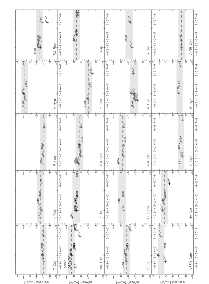
Figure 11: $\dot{M}$-estimates from Eq. 9 for the AGB stars in the sample. The dashed line indicates the mean value $\overline{\hbox{$\dot{M}$}}$ listed in Table LABEL:tbl:mdotestimates, the dashed line indicates the mean of the estimates. The shaded area indicates the typical uncertainty region around the mean value, which is a factor of three.

Fig. 11 (continued)

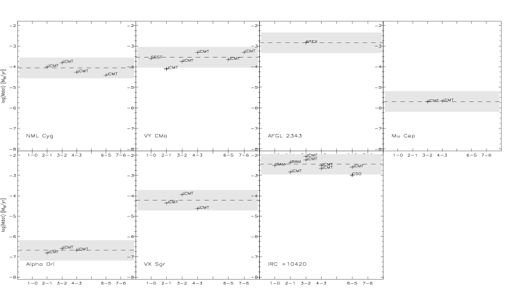
Figure 12: $\dot{M}$-estimates from Eq. 9 for the supergiants and hypergiants in the sample. The dashed line indicates the mean value $\overline{\hbox{$\dot{M}$}}$ listed in Table LABEL:tbl:mdotestimates, the dashed line indicates the mean of the estimates. The shaded area indicates the typical uncertainty region around the mean value, which is a factor of three.

5 Results and discussion

5.1 Mass-loss rate $\dot{M}$

For all targets in the sample for which we could fit at least one rotational line profile with a soft parabola (Eq. 2.3.1) we listed estimates for $\dot{M}$ in Table LABEL:tbl:mdotestimates. The estimates from all $\@element[12]{\mathrm{CO}}$ lines for the sample AGB stars are shown in Fig. 11. For the supergiants and hypergiants they are shown in Fig. 12. In case the soft-parabola fit procedure yielded a negative $\beta$, the exponent $s_{10,J}$ in Eq. 9 was assumed to be zero.

The listed estimates are averages over all values obtained via Eq. 9 for the fitted line transitions, and are written as $\overline{\hbox{$\dot{M}$}}$. In Table LABEL:tbl:mdotestimates we also listed the number of lines used and the spread of the estimates around the mean.

We did not attempt to fit the line profiles for U Ant and S Sct, since these are composed of emission from the inner part of the CSE and from the detached shell at larger outflow velocities, respectively. As discussed in Sect. 2.3.2 some other targets show clear deviations from the fitted soft-parabola profile. The estimates for these targets, e.g. EP Aqr, are therefore subject to larger uncertainties than the spreads listed in Table LABEL:tbl:mdotestimates and have to be interpreted with caution.

If the mass-loss-rate estimates of all available lines are within or close to the typical factor three uncertainty region, it is reasonable to state that the mass-loss rate of the target has been constant throughout the regions of the envelope sampled by these transitions. For most AGB stars in the sample this is indeed the case, but there are some exceptions indicating a possible variability in mass loss in the part of the envelope that is traced.

5.1.1 Variability

Criterion:

Since higher-$J$ transitions trace deeper, more recently formed envelope layers, a criterion to decide upon variability should consider the behaviour of the $\dot{M}$-estimates in view of the $J$-values. The presence of a picket-fence structure in the estimates, i.e. with $\dot{M}$ varying strongly between transitions could suggest variability of the mass-loss rate, but on rather short time scales of some hundreds of years. The presence of a strong overall gradient can also imply mass-loss-rate variability: e.g. decreasing $\dot{M}$ for increasing $J$ can be indicative for a mass-loss rate that has decreased over time. When discussing the sensitivity of our results to the modelling of the cooling of the envelope in Sect. 3.5.2, we pointed out that our estimates might intrinsically hold a shallow gradient. The differences associated with these model uncertainties between the highest and lowest estimates (for a constant $\dot{M}_{\mathrm{input}}$) are, however, not expected to exceed a factor three for $J=1-0$ up to $J=7-6$. Therefore, if a much steeper gradient is found in the estimates for some target, with a total coverage exceeding an order of magnitude in $\dot{M}$, we are therefore inclined to state that the mass-loss rate of the respective target has varied over time.

Variability in the sample:

The estimates for V669 Cas, shown in Fig. 11, exhibit the picket-fence type of trend and suggest that variability in the mass-loss rate is traced for this star.

The estimates for NV Aur and GLMP 1048 based on data of the $J=2-1,\,3-2,\,4-3,\,6-5$ transitions, the estimates for R Scl and IRC +20370, for $J=1-0,\,2-1,\,3-2,\,4-3,\,7-6$, and the estimates for CW Leo, for $J=1-0,\,2-1,\,3-2,\,4-3,\,6-5$ exhibit a spread of about an order of magnitude. This spread is within the uncertainties we expect around a $\dot{M}$-value and therefore points to a constant mass-loss rate throughout the traced regions of the envelope. The estimates for RW LMi, LP And and $\chi$ Cyg with $J=1-0,\,2-1,\,3-2,\,4-3,\,6-5$, respectively cover factors about ten, twenty and thirty in $\dot{M}$. The estimates for RX Boo, for $J=1-0,\,2-1,\,3-2,\,6-5$, cover a factor about forty in $\dot{M}$. In all these cases, we find a strong downward gradient, which most likely indicates that the more inward regions, i.e. the excitation regions of the higher-$J$ lines, were produced by a lower mass-loss rate than the outer regions. A strong gradient is also found for both WX Psc and LL Peg for $J=1-0$ up to $J=6-5$. For both targets, however, the $\dot{M}$-estimate based on the $J=7-6$ transition is higher by about an order of magnitude than the one based on the $J=6-5$ transition, indicating a recent increase of the mass-loss rate, as was proposed by Decin et al. (2007) for WX Psc. Qualitatively, this phenomenon is independent of the modelling of the H₂O-cooling, i.e. an increase would still be present if another cooling mechanism was considered in deriving the estimates. Obtaining a result corresponding to detailed modelling using an estimator as in Eq. 9 can be used as a benchmark for the quality of the estimator.

It is likely that the OH/IR stars and the more extreme Mira stars in the sample have already undergone mass-loss modulations, but to verify this more data are needed, especially of $J=1-0,\;6-5$ and $7-6$.

Data quality:

The IRAM measurements in our sample are subject to somewhat larger uncertainties than our own APEX and JCMT data since some questions have arisen about the data reduction. Decin et al. (2008Natureexlaba) already reported large uncertainties on the IRAM data of R Hya and Skinner et al. (1999) mentioned significant deviations between different measurements of the same lines towards CW Leo. The IRAM data Skinner et al. gathered from the literature and archives seemed to suffer from large uncertainties linked to pointing and calibration. They also discussed inconsistencies in the literature concerning the reported absolute line intensities. Very often confusion or unclarity arises about e.g. conversion from antenna temperatures to main-beam-brightness temperatures. For these reasons, we considered leaving the IRAM measurements out of the data set. In case of LL Peg this leads to a decrease of the estimated mass-loss rate with a factor 5.3, for IRC +20370 with a factor 3.9. For IRC +10420 and R Hya omitting the IRAM data has no effect on the $\dot{M}$-estimate. For the eight other objects with IRAM observations, the decrease is with a factor between 1.3 and 2.7. The $\dot{M}$-estimates ignoring IRAM data are always lower.

Omitting the IRAM data has an effect on the gradients seen in the estimates and discussed earlier. In many cases, the CO-sampling is now restricted to the transitions higher than $J=1-0$ and/or $J=2-1$, making possible trends less significant. In case of CW Leo, RX Boo, IRC +20370, RW LMi and LP And the supposed trends in the estimates are no longer present. For LL Peg the presence of an OSO $J=1-0$ measurement still gives the trend seen when the IRAM data are included.

For the oxygen-rich semi-regular variable RX Boo we find two estimates that could hint towards variability, i.e. those based on the IRAM $J=1-0$ and JCMT $J=6-5$ measurements. The latter is duplicated by a measurement carried out with CSO, and the estimate based on that observation is about an order of magnitude higher than the one derived from the JCMT. We are however inclined to attach more value to our JCMT observation, since the CSO calibration as described by Teyssier et al. (2006) holds larger uncertainties, such as rather large pointing errors. We conclude from this that there is some, however somewhat uncertain, downward trend with lower $\dot{M}$-estimates for higher $J$, indicating the possibility of a decrease in mass-loss rate over time.

Comparison to the literature:

Teyssier et al. (2006) note that a change in the mass-loss rate is needed to reproduce the data for three of their sample targets: R Hya, RW LMi and $\chi$ Cyg. Decin et al. (2008Natureexlaba) constructed a mass-loss model for R Hya and showed that a detached shell is needed to explain the rotation-vibrational lines. The purely rotational lines could however be reproduced with a constant mass-loss rate. Our estimates do, indeed, not point to any significant variations in the mass-loss rate, as can be seen from Fig. 11. The $\dot{M}$-estimates for RW LMi cover one order of magnitude and show a (shallow) gradient with lower $\dot{M}$ for higher $J$. This could point to a mass-loss rate that is presently lower than the one that produced the outer layers of the circumstellar envelope. Teyssier et al. specify a difference of only a factor 1.5 between the two mass-loss rates, so we can say that our estimates support this hypothesis of mass-loss-rate variability. In case of $\chi$ Cyg Teyssier et al. mention a minimum change of a factor 4 between the former and the present mass-loss rate, with the present one being lowest. This result is again reflected in our estimates.

The detached-shell structure of the carbon-rich semi-regular variable R Scl was described by Bergeat & Chevallier (2005) as the consequence of a former mass-loss rate of $\sim$$5.5\times 10^{-6}$ M_⊙  yr^-1 and a present mass-loss rate of $\sim$$3.5\times 10^{-7}$ M_⊙  yr^-1. The range of mass-loss rates covered by our estimates agrees with these values.

The mass-loss rates estimated from the individual CO emission lines for WX Psc — shown in Fig. 11 — are in very good agreement with the detailed modelling of the star by Decin et al. (2007). They present a profile $\dot{M}(r)$ exhibiting a high $\dot{M}$-value, followed in time by a strong decrease and again an increase of the mass-loss rate. We do not reproduce the same large difference of three orders in magnitude as mentioned by Decin et al. (2007). A possible explanation is that the excitation regions of the individual observed transitions are not restricted to either the high-$\dot{M}$ or the low-$\dot{M}$ regions. The estimates then represent more than one of these regions and are a kind of ’mean’ value of $\dot{M}$. However, the estimates we present in this paper for WX Psc reflect the detailed mass-loss modelling very well.

Winters et al. (2000) reported on possible time variability of the mass-loss rate of CW Leo. The present-day mass-loss rate is suggested to be lower than the mass-loss rate that produced the outer envelope layers by a factor of up to five. The decrease we see in our estimates, however, is by a factor $\sim$30. Also, the $\dot{M}$-values presented in the literature are about an order of magnitude higher than the $\overline{\dot{M}}$-value we derived. A possible explanation for these discrepancies is the H₂O-cooling uncertainty, leading to underestimates of $\dot{M}$. Another explanation is that the $J=7-6$ transition for the first time reveals a stronger variation in $\dot{M}$ than could be traced with single-dish observations of CO transitions up to $J=4-3$ or $6-5$. The model presented by Ramstedt et al. (2008) fitting lines $J=1-0$ up to $J=4-3$ shows clear deviations from the data. The discrepancies are systematic, i.e. the model underestimates the observed intensities more strongly for increasing $J$. This indicates the need for consideration of $\dot{M}$-variability for this target.

Neri et al. (1998) suggested that LL Peg might have a bipolar detached shell and Mauron & Huggins (2006) reported on a spiral structure in the envelope. The latter is indicative for variability in the outflow from the central star.

Supergiants and hypergiants:

The estimates for all five RSGs in our sample suggest constant mass-loss rates; see Fig. 12. In case of the yellow hypergiant IRC +10420, Humphreys et al. (1997); Castro-Carrizo et al. (2007) and Dinh-V.-Trung et al. (2009), among others, have put forward the possibility of a complex mass-loss history, with several episodes of high and low mass-loss rates. This resulted in multiple arc-like structures and shells around the central star. For AFGL 2343, the second hypergiant in our sample, we only used the $J=3-2$ line of $\@element[12]{\mathrm{CO}}$ to estimate the mass-loss rate, so no conclusions on variability in mass-loss rate can be drawn from this. Castro-Carrizo et al. (2007) mention variations in the mass-loss rate for both hypergiants on time scales of $\sim$1000 years. In this study, where we only consider CO emission lines measured with single-dish telescopes, we lack sensitivity for the rapid density fluctuations. This is due to the overlap of the line forming regions of the different rotational transitions.

(a) Histogram of the $\overline{\hbox{$\dot{M}$}}$-values for all AGB stars, grouped per pulsational type.

(b) Histogram of the $\overline{\hbox{$\dot{M}$}}$-values for all AGB stars, grouped per chemistry type. $N_{\mathrm{C}}$ is the number of carbon-rich targets, $N_{\mathrm{O}}$ is the number of oxygen-rich targets, and $N_{\mathrm{S}}$ is the number of S-type targets.

(c) Histogram of the $\overline{\hbox{$\dot{M}$}}$-values of all AGB stars.

Figure 13: Histograms containing the $\overline{\hbox{$\dot{M}$}}$-values estimated from Eq. 9 and given in Table LABEL:tbl:mdotestimates. The adopted bin size is $\Delta\log(\hbox{$\dot{M}$})=0.5$, which corresponds to about a factor three difference in mass-loss rate between consecutive bins.

5.1.2 AGB mass loss in view of pulsational type and chemistry type

The histograms in Fig. 13 show that the spread on $\overline{\hbox{$\dot{M}$}}$ for AGB stars is quite large, but there is a noticeable difference between the semi-regular variables on the one hand and the Miras and OH/IR targets on the other — see Fig. 13(a). The spread on $\dot{M}$ for the 16 Miras is rather extended, with values ranging from $9\times 10^{-8}$ M_⊙  yr^-1 (R Leo) up to $6\times 10^{-5}$ M_⊙  yr^-1 (NX Ser) and a mean value of $10^{-5}$ M_⊙  yr^-1.

The mass-loss rates for the 9 OH/IR targets were all estimated in the range $4\times 10^{-6}\leq\overline{\hbox{$\dot{M}$}}\leq 6\times 10^{-5}$ M_⊙  yr^-1, with an average of $2\times 10^{-5}$ M_⊙  yr^-1. The estimates for these targets seem low, considering that OH/IR stars have optically thick envelopes and can be heavily obscured. However, it has already been pointed out by e.g. Delfosse et al. (1997) that the mass-loss rates derived from CO lines can be significantly lower than those derived from the infrared flux in the case of OH/IR stars. The most likely explanation for the discrepancy is found in the recent ($\sim$1000 yr ago) onset of a superwind phase. The latter would not be traced by the CO lines available in this data set, except possibly for WX Psc.

The SRb targets have lower mass-loss rates, with an average of $5\times 10^{-7}$ M_⊙  yr^-1 and the highest value reaching $2\times 10^{-6}$ M_⊙  yr^-1 (R Scl). These results are in accordance with the idea that the SR variables are likely progenitors of Miras (Whitelock & Feast, 2000; Yeşilyaprak & Aslan, 2004).

When considering the histogram representing the AGB targets grouped per chemistry type (oxygen-rich, carbon-rich or S-type) in Fig. 13(b), no clear distinction between these groups can be made. Though this could be due to the bias of our sample towards oxygen-rich stars, there are no clear indications for significant discrepancies in $\dot{M}$ between the different types. Ramstedt et al. (2006) also reported no noticeable differences in $\dot{M}$-values for the different chemistries. Putting all AGB targets together for which $\dot{M}$-estimates could be made — irrespective of pulsational or chemical type — in Fig. 13(c), we get a minimum value of $4\times 10^{-8}$ M_⊙  yr^-1 (SRb V438 Oph), a maximum value of $6\times 10^{-5}$ M_⊙  yr^-1 (O-rich Mira NX Ser) and a mean of $10^{-5}$ M_⊙  yr^-1.

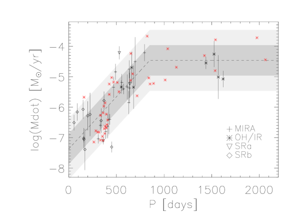
Figure 14: Mean estimates for $\dot{M}$ versus period of pulsation for the AGB stars in the sample are plotted in black. Different pulsational types are indicated with different plotting symbols: + for Miras, $\ast$ for OH/IR stars, $\nabla$ for SRa and $\diamond$ for SRb type stars. The red $\ast$ OH/IR data points were obtained from He & Chen (2001, priv. comm.). A linear relation fits the Miras, OH/IR stars and semi-regular variables in our sample with periods shorter than 850 days. $\dot{M}$ levels off to a constant value of $2.6\times 10^{-5}$ M_⊙  yr^-1 for longer periods. The darker shaded region represents a factor three spread around this fit, the paler grey region represents a spread of a factor 10. See Sect. 5.1.3 for further details.

5.1.3 AGB mass loss as a function of pulsation period

The $\overline{\hbox{$\dot{M}$}}$-values for all AGB stars in the sample — except for the RV Tauri star R Sct — are plotted versus pulsation period in Fig. 14 with error bars indicating the spread as listed in Table LABEL:tbl:mdotestimates. In case only one or two estimates could be obtained, we assumed a spread of a factor three, which is appropriate considering the overall spread in the sample. The red data points in the graph were taken from He & Chen (2001) and cover different types of OH/IR stars with a large spread on the periods of pulsation. Five objects in the sample of He & Chen (2001) are also present in our sample. Their pulsation periods and mass-loss rates are in accordance with our estimates, except in the case of V669 Cas, where He & Chen use $P=1995$ days (Slootmaker et al., 1985), while we adopted the more recently determined $P=1525$ days (Groenewegen et al., 1999). In constructing a linear relation between the pulsation period and the logarithm of the mass-loss rate, we only took into account the data points in our sample — i.e. we did not consider the data points of He & Chen (2001) — with periods shorter than 1000 days. The positions in the graph of the objects with periods longer than 850 days are represented by a constant $\dot{M}$ of $3.4\times 10^{-5}$ M_⊙  yr^-1. The linearly increasing part of the fit ($P\lesssim 850$ days) was constructed to represent the Miras, the short-period OH/IR stars and the AGB semi-regulars. The constant fitting value represents a levelling-off or saturation of the AGB mass-loss rate for stars with long periods, as proposed by, e.g., Vassiliadis & Wood (1993). The lack of data points for stars with longer periods complicates the determination of the cut-off period and the mean $\dot{M}$-value for the long-$P$ objects. Both were more or less arbitrarily chosen to yield a good fit. The fit in Fig. 14 is represented by

$$\begin{array}[]{lcllr}\log(\hbox{$\dot{M}$})&=&-7.37+3.42\times 10^{-3}\times P&&P\lesssim 850\,\mathrm{days}\\ &=&-4.46&&P\gtrsim 850\,\mathrm{days}\\ \end{array}$$

with $\dot{M}$ in units of M_⊙  yr^-1 and $P$ in days. Although He & Chen (2001) note that the quality of their derived mass-loss rates may be questionable, we find that their data points of both short and long-period targets are well represented by our fit. The targets that deviate strongest from the fit are semi-regular variables, e.g. W Hya and U Hya, and the Miras NX Ser (O-rich) and W Aql (S-type). We note that in constructing the fit we did not take into account the effect of differences in stellar mass that are likely to cause extra spread on the mass-loss rate for fixed pulsation periods, as shown by Vassiliadis & Wood (1993). We also point out the very good agreement between our fit and the results presented by Schöier & Olofsson (2001), who produced a similar diagram of $\dot{M}$ versus pulsation period for a sample of 68 optically bright carbon stars (their Fig. 12), and found a relation $\dot{M}\propto P^{2.3}$ for periods $P$ between 100 and 800 days.

Table 8: Line intensity ratios $I_{\mathrm{MB}}(^{12}\mathrm{CO})/I_{\mathrm{MB}}(^{13}\mathrm{CO})$ for the sample stars give first order estimates of their isotope abundance ratio $\@element[12]{\mathrm{C}}$/$\@element[13]{\mathrm{C}}$. An absolute flux error of $20\,\%$ for transitions $J=2-1,\;3-2$, and $4-3$ gives an error of $28\,\%$ on the respective line intensity ratios. For $J=6-5$, the absolute flux error is of the order of $30\,\%$, so the error on the line intensity ratio is about $42\,\%$. The $\@element[12]{\mathrm{C}}$/$\@element[13]{\mathrm{C}}$-value listed in the second to last column is the mean line intensity ratio, corrected with a factor 0.87 for the difference in line strengths (Eq. 15). The last column (M09) lists the values derived by Milam et al. (2009) from CO data.

	$I_{\mathrm{MB}}(^{12}\mathrm{CO})/I_{\mathrm{MB}}(^{13}\mathrm{CO})$					M09
Target	$2-1$	$3-2$	$4-3$	$6-5$	$\@element[12]{\mathrm{C}}$/$\@element[13]{\mathrm{C}}$	$\@element[12]{\mathrm{C}}$/$\@element[13]{\mathrm{C}}$
O-rich
RX Boo	12.0	10.5	-	-	9.8	-
EP Aqr	9.5	6.2	12.3	-	8.1	-
T Cet	11.5	14.4	-	-	11.2	-
o Cet	12.2	8.0	-	3.3	6.8	-
IK Tau	8.7	6.8	-	-	6.7	10
TX Cam	17.1	13.3	-	-	13.2	31
NV Aur	5.4	-	-	-	4.7	-
R Hya	6.1	-	-	-	5.3	-
R Cas	20.8	12.4	-	-	14.4	-
WX Psc	6.2	5.5	-	-	5.1	-
AFGL 5379	8.3	-	-	-	7.2	-
OH 44.8-2.3	3.8	7.6	-	-	4.9	-
NML Cyg	10.0	-	-	-	8.7	13
$\alpha$ Ori	6.5	-	-	-	5.7	8
VY CMa	19.7	14.3	-	-	14.8	25, 33, 46
VX Sgr	-	22.0	-	-	19.2	-
IRC +10420	9.0	9.7	-	-	8.1	14
AFGL 2343	-	3.8	-	-	3.3	-
S-type
$\pi^{1}$ Gru	-	35.3	-	-	30.7	-
W Aql	16.1	12.8	-	-	12.6	-
$\chi$ Cyg	-	16.2	-	-	14.1	33
C-rich
V Hya	-	30.7	-	-	26.7	71, 72
R Scl	-	10.6	-	-	9.2	-
II Lup	-	4.6	-	-	4.0	-
IRC +20370	-	8.1	-	-	7.1	-
V Cyg	13.8	-	-	-	12.0	-
LL Peg	-	4.2	-	-	3.6	-

Figure 15: Histogram with empirical estimates of the $\@element[12]{\mathrm{C}}$/$\@element[13]{\mathrm{C}}$ isotope abundance ratio for the AGB stars in our sample with an adopted bin size of two units. The targets are grouped per characteristic chemistry: carbon-rich objects (top panel), oxygen-rich targets (middle panel), and S-type targets (bottom panel).

5.2 $\@element[12]{\mathrm{C}}$/$\@element[13]{\mathrm{C}}$ isotope abundance ratio

For 29 sample stars we have observations of both $\@element[12]{\mathrm{CO}}$ and $\@element[13]{\mathrm{CO}}$ rotational lines, allowing us to estimate the $\@element[12]{\mathrm{C}}$/$\@element[13]{\mathrm{C}}$ isotope abundance ratio. This ratio is a tracer of the star’s chemical evolutionary state and nucleosynthesis (Sopka et al., 1989; Schöier & Olofsson, 2000; García-Hernández et al., 2007; Milam et al., 2009). $\@element[13]{\mathrm{C}}$ is produced during the interpulse phases when, after dredge-up, protons are partially mixed in the region between the hydrogen and helium burning shells. Reactions of the protons with $\@element[12]{\mathrm{C}}$ in this intershell region form $\@element[13]{\mathrm{C}}$. In massive AGB stars ($3$ M_⊙ $\leq$ $M_{\star}$ $\leq 7$ M_⊙), “hot bottom burning” (HBB) can be activated when the convective envelope penetrates the hydrogen-burning shell. During HBB, $\@element[12]{\mathrm{C}}$/$\@element[13]{\mathrm{C}}$ is lowered, since the net production of $\@element[13]{\mathrm{C}}$ is higher than that of $\@element[12]{\mathrm{C}}$ in the re-activated CN-cycle. For HBB-stars, a ratio $\@element[12]{\mathrm{C}}$/$\@element[13]{\mathrm{C}}$ around 10 is expected, but could possibly range down to values about 3 or even 1 (Ohnaka & Tsuji, 1999). HBB is expected to be active in the most massive and luminous oxygen-rich AGB stars. In this respect, OH/IR stars — typified by high luminosities, large infrared excesses and high mass-loss rates — are the best candidates for having very low $\@element[12]{\mathrm{C}}$/$\@element[13]{\mathrm{C}}$ isotope ratios (García-Hernández et al., 2007, and references therein).

Observational $\@element[12]{\mathrm{C}}$/$\@element[13]{\mathrm{C}}$-values for AGB stars range from as low as 1 (Ohnaka & Tsuji, 1999) up to about 90 (Milam et al., 2009). Lebzelter et al. (2008, and references therein) mention some clustering of empirical values of $\@element[12]{\mathrm{C}}$/$\@element[13]{\mathrm{C}}$ between 50 and 70 for galactic C-rich stars, while their evolutionary models even predict values higher than 100. The solar value is about 89 (Anders & Grevesse, 1989).

Line strength ratios of $\@element[12]{\mathrm{CO}}$ and $\@element[13]{\mathrm{CO}}$ transitions with identical $J$ provide a first order estimate of the isotope abundance ratio in case both lines are optically thin (Schöier & Olofsson, 2000). In case of optically thick lines, these estimates are only tentative, and lower than the actual isotopic ratio. Schöier & Olofsson (2000) mention that the $\@element[12]{\mathrm{C}}$/$\@element[13]{\mathrm{C}}$ values derived from their radiative transfer models are mostly higher than those estimated from intensity ratios. This effect is largest for their high $\dot{M}$-objects, where the difference amounts to a factor 6.

We note here that the line intensity ratios for $J=2-1$ are consistently larger than those for $J=3-2$ for our sample stars. A linear least-squares fit for the targets with line intensity ratios available for both $J=2-1$ and $J=3-2$ shows that

$$\frac{I(^{12}\mathrm{CO}(3-2))}{I(^{13}\mathrm{CO}(3-2))}=4.3+0.48\times\frac{I(^{12}\mathrm{CO}(2-1))}{I(^{13}\mathrm{CO}(2-1))}.$$

The standard deviation from this linear fit is 2.1 units in $I(^{12}\mathrm{CO}(3-2))/I(^{13}\mathrm{CO}(3-2))$. The slope and offset in this relation clearly indicate that individual line intensity ratios will not lead to accurate values of the actual $\@element[12]{\mathrm{C}}$/$\@element[13]{\mathrm{C}}$ abundance ratio and can only give rough estimates.

We have calculated $\@element[12]{\mathrm{C}}$/$\@element[13]{\mathrm{C}}$-values for our sample targets, correcting for line strength differences and — for the sake of simplicity — assuming the targets were unresolved by the beam, in the way this was done by Schöier & Olofsson (2000) and as is given by Eq. 15.

$$^{12}\mathrm{C}/^{13}\mathrm{C}=\frac{I_{\mathrm{MB}}(^{12}\mathrm{CO}(J\rightarrow J-1))}{I_{\mathrm{MB}}(^{13}\mathrm{CO}(J\rightarrow J-1))}\times\left(\frac{\nu_{{}^{12}\mathrm{CO}(J\rightarrow J-1)}}{\nu_{{}^{13}\mathrm{CO}(J\rightarrow J-1)}}\right)^{-3}$$ (15)

The frequency correction factor is equal to 0.87 for all values of $J$ considered. If multiple line intensity ratios were available for one $J$, these were averaged. The line intensity ratios and the resulting values for $\@element[12]{\mathrm{C}}$/$\@element[13]{\mathrm{C}}$ are listed in Table 8. Fig. 15 shows a histogram plot of the $\@element[12]{\mathrm{C}}$/$\@element[13]{\mathrm{C}}$-values for the AGB stars in the sample. It is clear from this graph that we derive very low values for $\@element[12]{\mathrm{C}}$/$\@element[13]{\mathrm{C}}$, but as mentioned before, these estimates are lower limits in case of large mass-loss rate objects due to optical depth effects, that are not taken into account using this approach. Since high-$\dot{M}$ objects are more easily observed, the sample is biased towards the higher mass-loss rates. The values for the 12 Miras range from 3.6 (carbon-rich LL Peg) up to 14.4 (oxygen-rich R Cas) and for the 3 OH/IR stars they range from 4.9 (OH 44.8-2.3) up to 7.2 (AFGL 5379). The spread on $\@element[12]{\mathrm{C}}$/$\@element[13]{\mathrm{C}}$ for the other stars in the sample is quite large and we do not see any clear differences in the first-order estimates of $\@element[12]{\mathrm{C}}$/$\@element[13]{\mathrm{C}}$ when considering the different types of stars in the sample.

Milam et al. (2009) found $\@element[12]{\mathrm{C}}$/$\@element[13]{\mathrm{C}}$ $\sim$13 for NML Cyg and $\@element[12]{\mathrm{C}}$/$\@element[13]{\mathrm{C}}$ $\sim$14 for IRC +10420, while for VY CMa they derived a much higher value between 25 and 46. We find similar ratios with a first order estimate for VY CMa of 14.8, and values of 8.7 and 8.1 for NML Cyg and IRC +10420, respectively. We note that Milam et al. (2009) deconvolved the line profiles for VY CMa and V Hya into separate velocity components, since the different structures probed could have discrepant chemical properties (see also Ziurys et al., 2007, for VY CMa). They analysed the multiple components for $\@element[12]{\mathrm{C}}$/$\@element[13]{\mathrm{C}}$ separately, resulting in three different values for VY CMa (46, 33 and 25) and 2 values for V Hya (71 and 72). Milam et al. (2009) claim a $\pm 30$ % uncertainty on their $\@element[12]{\mathrm{C}}$/$\@element[13]{\mathrm{C}}$-values.

5.3 Wind driving efficiency

Figure 16: Comparative histogram plots of the expansion velocities ($v_{\infty}$) of the AGB stars in the sample. The bin size was set to $\Delta\hbox{$v_{\infty}$}=2.5$ km s^-1. The targets are grouped per characteristic chemistry: carbon-rich objects (top panel), oxygen-rich targets (middle panel), and S-type targets (bottom panel).

Olofsson et al. (1993) and Oudmaijer et al. (2008) suggest that the acceleration of winds around C-rich stars is more efficient than that of winds around O-rich stars because of differences in dust absorption properties. Comparing samples of 40 S-type, 77 oxygen-rich and 61 carbon-rich stars, Ramstedt et al. (2006) also find indications for a higher terminal velocity in carbon-rich stars.

Fig. 16 shows histograms of $v_{\infty}$ in our sample for the three different chemical types of objects: oxygen-rich, carbon-rich and S-type stars. The mean $v_{\infty}$-values for respectively 24 oxygen-rich and 13 carbon-rich AGB targets in our sample are 14.5 km s^-1 and 15.4 km s^-1. These values are $\sim$4–10 km s^-1 higher than those of Ramstedt et al. (2006). We note that the largest $v_{\infty}$-values for our carbon-rich and S-type sample exceed those of Ramstedt et al. (2006) by about 10 km s^-1. These extreme values are however the only ones in both samples — V Hya in the C-rich and $\pi^{1}$ Gru in the S-type sample — so they are only weakly reflected in the samples’ mean values. Our results do not lead to the same clear conclusion that the wind driving efficiency is higher for carbon-rich than for oxygen-rich stars. They do, however, point in the same direction considering the sampling bias we have in favour of oxygen-rich objects and the occurrence of higher $v_{\infty}$-values for carbon-rich than for oxygen-rich targets in our sample.

6 Conclusions

The data set presented in this paper covers a very large number of high-quality measurements of CO rotational line transitions $J\rightarrow J-1$ with $J$ ranging from 1 up to 7. Observations of both $\@element[12]{\mathrm{CO}}$ and $\@element[13]{\mathrm{CO}}$ are included. It is the first time that a CO data set allowing one for such a detailed sampling of circumstellar envelopes of evolved objects is presented in the literature.

A grid of radiative transfer models calculated with GASTRoNOoM covering AGB stellar and wind parameters was used to derive a formalism allowing one to make estimates of mass-loss rates. The $\dot{M}$-estimator is valid for $J$ up to 16, while until now, only estimators valid for $J$ up to 4 have been presented in the literature. We also extended the validity range of the $\dot{M}$-estimator by correcting for saturation of the CO line intensities and therefore accounting for optically thick winds. The intrinsic spread of the estimator ensures good $\dot{M}$-estimates when all input parameters are well determined. We like to point out that, when only one transition is used to estimate a mass-loss rate, the $J=2-1$ transition will give the most reliable results.

For many of the sample AGB stars, the estimates based on the different rotational lines result in constant $\dot{M}$-values. The estimates for 7 targets do however hint at a variability of the mass-loss rate, by showing a large spread (more than an order of magnitude in $\dot{M}$) and clear trends. Uncertainties linked to the implemented H₂O-cooling could produce the effect of seemingly decreasing $\dot{M}$ in time, but there are two convincing cases in which these uncertainties cannot account for the variations seen in the estimates. This is the case for LL Peg and WX Psc, and we have shown that the $\dot{M}$-estimates for the latter target reflect the mass-loss history constructed through detailed radiative-transfer modelling by Decin et al. (2007). The fact that we (1) do not have full sampling of all rotational $J$-levels for all sample targets and that (2) did not perform full radiative-transfer modelling for the sample, of course limit our ability to prove conclusively that a star has experienced a constant mass loss or mass-loss modulations. This kind of detailed modelling will be presented in a forthcoming paper by Lombaert et al. (in preparation). The examples discussed in this paper show, however, that the use of the estimator allows one not only to establish good mass-loss-rate estimates in case of constant mass-loss targets, but also to trace strong variability in the mass-loss rate of AGB stars, given a sufficiently large number of CO line transitions. The fact that our estimates bear quite close resemblance to the mass loss derived through detailed radiative transfer modelling, gives confidence that our estimator is of good quality.

Further observations of mostly high-excitation rotational lines, such as $J=6-5$ and $J=7-6$ would make it possible to make a better distinction between constant or (possibly) variable mass loss. The $J=5-4$ transition will be measured by HIFI for many stars in our sample. These additional measurements will provide a more complete sampling of the circumstellar envelopes and the mass-loss history of these evolved stars.

Appendix A CO data – figures and tables

All $\@element[12]{\mathrm{CO}}$ and $\@element[13]{\mathrm{CO}}$ data of the sample and the soft-parabola fits (Sect. 2.3.1) to these data are shown in Figs. 17 and 18. The most important line parameters — main-beam temperature at the line centre and integrated intensity — and the $\beta$ parameter from the soft-parabola fitting procedure as described in Sect. 2.3.1 are given in Tables LABEL:tbl:12CO and LABEL:tbl:13CO. References for, or remarks on, the data are listed in Tables LABEL:tbl:12CO-REMARKS and LABEL:tbl:13CO-REMARKS for the $\@element[12]{\mathrm{CO}}$ and $\@element[13]{\mathrm{CO}}$ data respectively.

1

Table 9: Overview of all data presented in Fig. 17. The objects are ordered according to their IRAS numbers and are specified with their velocity in the frame of the Local Standard of Rest ($v_{\mathrm{LSR}}$) and the terminal velocity ($v_{\infty}$) of the CO envelope. For each measured transition, the main beam brightness temperature at the centre of the line ($T_{\mathrm{MB,c}}$) is given in K, together with the integrated intensity ($I_{\mathrm{MB}}$), given in K km s^-1. For the high-quality data, a soft parabola fit (see text) was performed and the according $\beta$-values are listed as the third entry per transition. In case of multiple observations of a specific transition, the data are given in the exact same order as in Fig. 17.

IRAS	Alternative name	$v_{\mathrm{LSR}}$	$v_{\infty}$	CO 1–0			CO 2–1			CO 3–2			CO 4–3			CO 6–5			CO 7–6
		km/s		$T_{\mathrm{MB,c}}$	$I_{\mathrm{MB}}$	$\beta$	$T_{\mathrm{MB,c}}$	$I_{\mathrm{MB}}$	$\beta$	$T_{\mathrm{MB,c}}$	$I_{\mathrm{MB}}$	$\beta$	$T_{\mathrm{MB,c}}$	$I_{\mathrm{MB}}$	$\beta$	$T_{\mathrm{MB,c}}$	$I_{\mathrm{MB}}$	$\beta$	$T_{\mathrm{MB,c}}$	$I_{\mathrm{MB}}$	$\beta$
-	NML Cyg	2.0	33.0	-	-	-	2.17	94.68	1.42	4.23	197.40	1.10	2.68	128.60	1.27	2.30	110.97	1.45	-	-	-
00192-2020	T Cet	23.0	7.0	-	-	-	0.35	3.91	1.45	0.69	7.18	1.12	0.95	10.12	1.45	0.73	8.26	1.14	-	-	-
01037+1219	WX Psc	9.0	19.8	0.19	3.61	1.10	2.29	65.64	1.53	2.98	80.79	1.95	1.88	49.81	2.16	0.54	8.59	2.15	0.86	22.78	2.27
”	”	”	”	0.55	51.70	0.84	1.64	59.76	0.26	2.44	66.43	1.72	1.42	40.76	1.56	-	-	-	1.06	34.78	0.59
”	”	”	”	0.92	25.45	0.99	2.11	59.32	1.47	2.43	67.15	1.60	1.44	40.21	1.66	-	-	-	0.90	36.45	0.15
”	”	”	”	0.91	26.95	0.80	-	-	-	-	-	-	-	-	-	-	-	-	-	-	-
01246-3248	R Scl	-17.0	17.0	0.98	24.86	1.21	1.73	47.60	0.70	1.72	54.69	-0.22	1.21	45.70	-0.77	-	-	-	0.99	25.91	-0.33
01304+6211	V669 Cas	-55.0	13.0	-	-	-	0.28	1.72	2.80	0.68	10.77	1.99	0.14	2.12	0.08	0.35	7.12	-0.49	-	-	-
02168-0312	o Cet	46.4	8.1	1.25	8.09	6.89	13.79	63.74	17.16	21.76	107.17	15.33	20.01	101.63	12.43	16.25	86.23	9.81	-	-	-
03507+1115	IK Tau	33.8	18.5	1.68	63.35	-0.75	4.54	150.35	0.23	3.04	87.02	0.99	4.36	127.27	0.92	-	-	-	5.04	122.61	1.91
”	”	”	”	-	-	-	2.93	89.62	0.54	4.04	115.71	1.01	4.25	119.43	1.09	-	-	-	-	-	-
”	”	”	”	-	-	-	5.97	200.84	0.12	3.23	94.22	1.01	-	-	-	-	-	-	-	-	-
04566+5606	TX Cam	10.8	21.2	-	-	-	2.34	63.58	2.10	5.41	144.84	2.22	2.77	76.30	2.24	-	-	-	-	-	-
05073+5248	NV Aur	3.0	19.2	-	-	-	1.38	36.31	1.75	1.51	38.76	1.91	1.35	35.43	2.21	0.37	8.88	1.10	-	-	-
05524+0723	Alpha Ori	3.5	14.0	-	-	-	0.02	-0.29	-	1.98	49.06	0.25	2.60	60.01	0.65	-	-	-	-	-	-
”	”	”	”	-	-	-	0.66	16.00	0.06	-	-	-	-	-	-	-	-	-	-	-	-
06176-1036	Red Rectangle	0.3	8.3	-	-	-	-	-	-	0.84	4.60	16.94	-	-	-	-	-	-	-	-	-
07209-2540	VY CMa	21.0	46.5	0.07	44.20	10.48	0.98	65.40	1.59	2.85	171.76	2.00	6.48	405.72	1.84	4.84	247.31	3.69	7.65	423.46	3.12
07399-1435	Calabash Nebula	40.0	110.0	-	-	-	-	-	-	1.73	111.03	19.67	-	-	-	-	-	-	-	-	-
09448+1139	R Leo	-1.0	9.0	0.37	4.07	2.01	2.19	28.43	1.81	2.99	33.54	2.93	-	-	-	4.46	38.10	4.49	-	-	-
”	”	”	”	-	-	-	-	-	-	1.89	22.63	1.47	-	-	-	-	-	-	-	-	-
09452+1330	CW Leo	-25.0	14.5	17.44	411.94	0.53	38.17	830.58	1.04	40.92	852.24	1.36	30.08	639.17	1.40	58.25	1130.61	1.92	-	-	-
”	”	”	”	9.68	222.79	0.99	23.27	491.83	2.13	31.98	672.09	1.41	-	-	-	-	-	-	-	-	-
”	”	”	”	9.49	230.77	0.38	-	-	-	-	-	-	-	-	-	-	-	-	-	-	-
10131+3049	RW LMi	-1.8	20.8	4.10	132.65	0.77	7.75	215.61	1.94	3.02	74.82	3.04	4.21	126.23	2.04	7.03	182.66	2.77	-	-	-
10197-5750	GSC 08608-00509	-5.0	28.0	-	-	-	-	-	-	0.75	24.76	3.09	-	-	-	-	-	-	-	-	-
10329-3918	U Ant	24.0	20.5	0.22	9.96	-	0.32	11.53	-	0.50	9.59	-	0.33	2.76	-	-	-	-	0.05	-4.69	-
10350-1307	U Hya	-31.0	8.5	0.42	4.79	1.72	0.91	10.76	4.28	2.64	29.28	2.51	2.94	30.64	2.81	-	-	-	3.29	25.13	5.11
10491-2059	V Hya	-17.0	30.0	0.81	22.93	7.12	1.47	37.99	8.87	3.47	105.43	5.42	1.53	53.47	3.75	-	-	-	1.31	16.81	-
12427+4542	Y CVn	21.0	7.5	0.93	9.07	0.87	1.88	24.62	0.43	-	-	-	1.36	17.00	0.37	1.25	16.85	0.48	-	-	-
13269-2301	R Hya	-10.0	12.5	0.13	1.58	5.23	1.11	13.00	5.51	4.01	41.49	7.76	-	-	-	6.44	51.68	13.55	-	-	-
”	”	”	”	-	-	-	1.42	17.02	5.82	1.64	14.82	9.03	-	-	-	-	-	-	-	-	-
”	”	”	”	-	-	-	0.69	6.35	6.31	-	-	-	-	-	-	-	-	-	-	-	-
13428-6232	GLMP 363	-	-	-	-	-	-	-	-	-0.00	2.41	-	-	-	-	-	-	-	-	-	-
13462-2807	W Hya	41.0	8.5	-	-	-	-	-	-	2.61	36.50	0.44	3.06	41.08	0.95	-	-	-	3.06	32.06	2.21
14219+2555	RX Boo	2.0	9.0	1.10	16.47	0.53	3.19	50.12	0.36	3.93	58.09	0.60	-	-	-	0.43	4.13	4.60	-	-	-
”	”	”	”	-	-	-	2.06	30.97	0.70	1.54	23.30	0.75	-	-	-	2.57	30.02	3.05	-	-	-
15194-5115	II Lup	-15.0	23.0	-	-	-	-	-	-	4.66	144.41	1.64	4.93	155.90	1.61	-	-	-	4.89	151.43	1.77
”	”	”	”	-	-	-	-	-	-	4.55	144.38	1.52	3.96	128.39	1.40	-	-	-	3.18	82.09	3.28
16262-2619	Alpha Sco	-	-	-	-	-	-	-	-	0.02	0.46	-	-	-	-	-	-	-	-	-	-
16269+4159	G Her	20.4	13.0	-	-	-	0.41	6.15	4.29	1.33	23.21	3.30	-	-	-	1.18	17.02	2.88	-	-	-
17123+1107	V438 Oph	9.8	4.2	-	-	-	0.20	1.19	1.99	0.31	1.60	1.75	-	-	-	-	-	-	-	-	-
17150-3224	Cotton Candy Nebula	15.0	24.0	-	-	-	-	-	-	0.78	18.84	5.15	-	-	-	-	-	-	-	-	-
17411-3154	AFGL 5379	-21.2	25.0	-	-	-	1.59	49.95	2.65	2.81	80.36	3.41	2.36	64.80	3.38	-	-	-	1.83	54.44	3.00
”	”	”	”	-	-	-	-	-	-	1.76	50.45	3.48	-	-	-	-	-	-	-	-	-
17443-2949	PN RPZM 39	-	-	-	-	-	-	-	-	0.24	5.26	-	-	-	-	-	-	-	-	-	-
17501-2656	V4201 Sgr	-	-	-	-	-	0.52	1.00	-	0.30	0.11	-	-	-	-	-	-	-	-	-	-
18050-2213	VX Sgr	6.5	24.3	-	-	-	0.74	32.47	0.30	2.41	94.47	0.73	1.18	42.12	0.95	-	-	-	-	-	-
18059-3211	Gomez Nebula	2.7	6.0	-	-	-	0.47	2.79	3.86	0.91	4.37	8.95	-	-	-	-	-	-	-	-	-
18100-1915	OH 11.52 -0.58	-	-	-	-	-	-	-	-	-0.60	-3.27	-	0.02	1.91	-	-	-	-	-0.66	0.07	-
18257-1000	V441 Sct	115.0	-	-	-	-	-	-	-	0.23	2.94	-	0.13	4.76	-	-	-	-	-0.06	-7.52	-
18308-0503	AFGL 5502	43.0	14.7	-	-	-	43.96	253.44	40.33	45.72	289.44	33.42	52.00	301.50	38.30	16.27	94.75	34.52	-	-	-
18327-0715	OH 24.69 +0.24	40.0	-	-	-	-	-	-	-	-0.09	-7.40	-	-0.10	-2.95	-	-	-	-	0.91	-1.46	-
18333+0533	NX Ser	33.5	17.8	-	-	-	1.20	26.08	2.72	1.29	28.15	3.16	0.97	22.02	1.96	0.20	4.09	2.49	-	-	-
18348-0526	OH 26.5+0.6	27.4	17.0	-	-	-	-0.18	7.02	-	1.09	23.57	2.19	0.85	18.98	1.85	-	-	-	-	-	-
18361-0647	OH 25.50 -0.29	27.5	-	-	-	-	-	-	-	1.76	3.29	-	2.31	6.62	-	-	-	-	0.05	1.57	-
18397+1738	IRC +20370	-0.5	16.0	3.65	84.14	1.12	4.52	93.39	2.07	2.93	60.34	2.21	3.45	66.09	2.85	-	-	-	3.10	49.77	3.51
18432-0149	V1360 Aql	40.0	-	-	-	-	-	-	-	-0.41	6.38	-	-1.23	-2.43	-	-	-	-	1.47	-5.88	-
18448-0545	R Sct	57.0	6.0	-	-	-	-	-	-	0.77	3.85	8.17	-	-	-	-	-	-	-	-	-
18460-0254	V1362 Aql	100.0	-	-	-	-	0.32	18.17	-	-0.35	6.81	-	0.02	-5.16	-	-	-	-	0.16	1.21	-
”	”	”	”	-	-	-	-	-	-	-0.30	-7.24	-	-	-	-	-	-	-	-	-	-
18476-0758	S Sct	15.0	8.0	0.13	1.27	-	0.12	1.23	-	0.20	1.54	-	-	-	-	-	-	-	-	-	-
18488-0107	V1363 Aql	75.0	-	-	-	-	-	-	-	2.21	18.75	-	0.64	9.98	-	-	-	-	0.01	-0.29	-
18498-0017	V1365 Aql	60.0	-	-	-	-	0.35	10.72	-	0.36	13.07	-	0.34	8.50	-	-	-	-	-0.12	1.11	-
”	”	”	”	-	-	-	-	-	-	0.07	3.99	-	-	-	-	-	-	-	-	-	-
19067+0811	V1368 Aql	60.0	-	-	-	-	-	-	-	-0.62	1.50	-	-0.51	0.44	-	-	-	-	0.01	5.61	-
19110+1045	KJK G45.07	60.0	25.0	-	-	-	-	-	-	-	-	-	32.42	729.07	6.42	-	-	-	-	-	-
19114+0002	V1427 Aql	99.0	40.0	-	-	-	-	-	-	1.69	84.28	2.47	-	-	-	-	-	-	-	-	-
19126-0708	W Aql	-25.0	20.0	0.97	27.03	0.93	2.76	80.88	1.16	3.89	96.71	2.51	4.70	119.33	2.32	-	-	-	4.97	134.55	1.49
”	”	”	”	0.99	26.93	1.71	1.88	51.58	2.13	4.75	118.44	2.51	4.06	97.28	2.21	-	-	-	1.73	29.21	0.31
”	”	”	”	1.27	34.06	1.77	-	-	-	5.02	127.23	2.26	4.08	96.31	1.07	-	-	-	-	-	-
”	”	”	”	-	-	-	-	-	-	2.16	52.98	2.49	-	-	-	-	-	-	-	-	-
19192+0922	OH 44.8-2.3	-70.5	17.7	-	-	-	0.38	9.67	1.42	0.63	15.40	1.99	0.41	9.99	1.50	0.53	9.59	2.57	-	-	-
19244+1115	IRC +10420	75.5	42.3	0.90	49.94	2.10	1.61	94.76	1.44	3.23	178.76	1.93	2.94	149.88	2.72	2.77	139.62	2.46	-	-	-
”	”	”	”	-	-	-	2.46	158.99	0.87	3.75	227.95	1.73	2.10	118.49	1.81	1.63	80.74	2.08	-	-	-
19283+1944	AFGL 2403	29.0	17.0	-	-	-	0.54	10.48	3.01	0.24	5.53	2.30	0.40	8.83	2.43	-	-	-	-	-	-
19486+3247	Chi Cyg	10.5	8.5	3.20	35.55	0.38	6.32	90.86	0.26	3.49	47.70	0.75	10.25	125.99	1.30	1.45	23.08	0.14	-	-	-
”	”	”	”	0.80	10.01	1.06	4.11	57.77	0.60	5.32	75.11	0.61	-	-	-	-	-	-	-	-	-
”	”	”	”	-	-	-	-	-	-	5.46	75.53	0.62	-	-	-	-	-	-	-	-	-
20075-6005	X Pav	-18.5	11.0	-	-	-	-	-	-	1.24	20.18	1.14	-	-	-	-	-	-	-	-	-
20077-0625	IRC -10529	-18.0	16.5	-	-	-	-	-	-	1.91	36.97	3.27	1.56	33.48	2.13	-	-	-	0.49	19.74	-
20120-4433	RZ Sgr	-30.0	9.0	-	-	-	-	-	-	1.13	12.76	1.92	0.80	9.78	1.99	-	-	-	0.03	-1.88	-
20396+4757	V Cyg	15.0	15.0	-	-	-	2.65	43.61	2.62	-	-	-	-	-	-	-	-	-	-	-	-
21419+5832	Mu Cep	23.0	35.0	-	-	-	0.04	2.63	-	0.23	13.46	0.85	0.44	28.31	-0.20	-	-	-	-	-	-
21439-0226	EP Aqr	-33.5	11.5	-	-	-	5.12	30.07	75.47	7.88	42.15	72.53	7.94	42.19	68.50	7.33	31.35	99.32	-	-	-
21554+6204	GLMP 1048	-18.7	18.6	-	-	-	0.53	12.23	2.74	0.54	10.22	3.82	0.26	4.42	5.65	0.07	1.20	3.17	-	-	-
22177+5936	OH 104.9+2.4	-26.0	18.3	-	-	-	0.20	5.09	1.46	0.46	10.56	2.39	0.11	3.37	0.61	0.22	6.50	0.44	-0.54	-10.81	-
22196-4612	pi1 Gru	-11.0	30.0	-	-	-	-	-	-	3.84	99.14	9.01	3.32	79.75	10.77	-	-	-	1.81	39.85	8.23
23166+1655	LL Peg	-31.0	16.0	4.75	101.41	2.02	6.45	118.99	3.23	4.50	76.16	4.00	4.85	87.58	3.43	1.02	22.40	1.95	7.79	152.69	2.73
”	”	”	”	1.56	26.97	2.61	-	-	-	2.40	40.23	3.53	4.03	72.19	3.28	-	-	-	-	-	-
23320+4316	LP And	-17.0	14.0	4.28	83.92	1.16	7.90	153.59	1.72	3.81	67.60	2.25	4.14	74.17	2.34	3.09	54.90	1.85	-	-	-
”	”	”	”	1.63	33.70	0.94	-	-	-	-	-	-	-	-	-	-	-	-	-	-	-
23558+5106	R Cas	25.5	13.5	-	-	-	2.68	56.45	1.14	5.20	99.03	2.08	6.05	109.97	2.21	5.01	76.20	3.42	-	-	-

2

Table 10: References for the presented $\@element[12]{\mathrm{CO}}$ data. In case of multiple observations of a specific transition, the data are given in the exact same order as in Fig. 17. References or remarks are (1) Knapp & Morris (1985), (2) Margulis et al. (1990), (3) Nyman et al. (1992), (4) Sopka et al. (1989), (5) Knapp et al. (1982), (6) Olofsson et al. (1993), (7) Neri et al. (1998), (8) archive data, (9) Teyssier et al. (2006), (10) Groenewegen et al. (1998), (11) Huggins et al. (1988), (12) Wang et al. (1994), (13) Wannier & Sahai (1986), (14) Bieging & Latter (1994), (-) this study.

IRAS	Alternative name	CO 1–0		CO 2–1		CO 3–2		CO 4–3		CO 6–5		CO 7–6
		Telescope	Reference	Telescope	Reference	Telescope	Reference	Telescope	Reference	Telescope	Reference	Telescope	Reference
-	NML Cyg	-	-	JCMT	-	JCMT	-	JCMT	-	JCMT	-	-	-
00192-2020	T Cet	-	-	JCMT	-	JCMT	-	JCMT	-	JCMT	-	-	-
01037+1219	WX Psc	BLT	1	JCMT	-	JCMT	-	JCMT	-	JCMT	-	JCMT	-
”	”	FCRAO	2	OVRO	5	APEX	-	APEX	-	-	-	APEX	-
”	”	OSO	3	JCMT	-	APEX	-	APEX	-	-	-	APEX	-
”	”	OSO	4	-	-	-	-	-	-	-	-	-	-
01246-3248	R Scl	SEST	6	SEST	6	APEX	-	APEX	-	-	-	APEX	-
01304+6211	V669 Cas	-	-	JCMT	-	JCMT	-	JCMT	-	JCMT	-	-	-
02168-0312	o Cet	SEST	3	JCMT	-	JCMT	-	JCMT	-	JCMT	-	-	-
03507+1115	IK Tau	IRAM	7	IRAM	7	APEX	-	JCMT	8	-	-	APEX	-
”	”	-	-	JCMT	8	JCMT	8	APEX	-	-	-	-	-
”	”	-	-	IRAM	-	APEX	-	-	-	-	-	-	-
04566+5606	TX Cam	-	-	JCMT	-	JCMT	-	JCMT	-	-	-	-	-
05073+5248	NV Aur	-	-	JCMT	-	JCMT	-	JCMT	-	JCMT	-	-	-
05524+0723	Alpha Ori	-	-	JCMT	-	JCMT	-	JCMT	-	-	-	-	-
”	”	-	-	JCMT	8	-	-	-	-	-	-	-	-
06176-1036	Red Rectangle	-	-	-	-	APEX	-	-	-	-	-	-	-
07209-2540	VY CMa	SEST	3	JCMT	-	JCMT	-	JCMT	-	JCMT	-	JCMT	-
07399-1435	Calabash Nebula	-	-	-	-	APEX	-	-	-	-	-	-	-
09448+1139	R Leo	IRAM	9	IRAM	9	APEX	-	-	-	CSO	9	-	-
”	”	-	-	-	-	CSO	9	-	-	-	-	-	-
09452+1330	CW Leo	IRAM	10	IRAM	10	JCMT	10	CSO	9	CSO	9	-	-
”	”	NRAO	11	SEST	6	CSO	12	-	-	-	-	-	-
”	”	SEST	6	-	-	-	-	-	-	-	-	-	-
10131+3049	RW LMi	IRAM	9	IRAM	9	CSO	9	CSO	9	CSO	9	-	-
10197-5750	GSC 08608-00509	-	-	-	-	APEX	-	-	-	-	-	-	-
10329-3918	U Ant	SEST	6	SEST	6	APEX	-	APEX	-	-	-	APEX	-
10350-1307	U Hya	SEST	6	SEST	6	APEX	-	APEX	-	-	-	APEX	-
10491-2059	V Hya	SEST	6	SEST	6	APEX	-	APEX	-	-	-	APEX	-
12427+4542	Y CVn	IRAM	7	IRAM	7	-	-	CSO	9	CSO	9	-	-
13269-2301	R Hya	IRAM	9	IRAM	9	JCMT	-	-	-	CSO	9	-	-
”	”	-	-	JCMT	-	CSO	9	-	-	-	-	-	-
”	”	-	-	NRAO	13	-	-	-	-	-	-	-	-
13428-6232	GLMP 363	-	-	-	-	APEX	-	-	-	-	-	-	-
13462-2807	W Hya	-	-	-	-	APEX	-	APEX	-	-	-	APEX	-
14219+2555	RX Boo	IRAM	9	IRAM	9	JCMT	-	-	-	JCMT	-	-	-
”	”	-	-	JCMT	-	CSO	9	-	-	CSO	9	-	-
15194-5115	II Lup	-	-	-	-	APEX	-	APEX	-	-	-	APEX	-
”	”	-	-	-	-	APEX	-	APEX	-	-	-	APEX	-
16262-2619	Alpha Sco	-	-	-	-	JCMT	-	-	-	-	-	-	-
16269+4159	G Her	-	-	JCMT	-	JCMT	-	-	-	JCMT	-	-	-
17123+1107	V438 Oph	-	-	JCMT	-	JCMT	-	-	-	-	-	-	-
17150-3224	Cotton Candy Nebula	-	-	-	-	APEX	-	-	-	-	-	-	-
17411-3154	AFGL 5379	-	-	JCMT	-	JCMT	-	APEX	-	-	-	APEX	-
”	”	-	-	-	-	APEX	-	-	-	-	-	-	-
17443-2949	PN RPZM 39	-	-	-	-	JCMT	-	-	-	-	-	-	-
17501-2656	V4201 Sgr	-	-	JCMT	-	JCMT	-	-	-	-	-	-	-
18050-2213	VX Sgr	-	-	JCMT	-	JCMT	-	JCMT	-	-	-	-	-
18059-3211	Gomez Nebula	-	-	JCMT	-	JCMT	-	-	-	-	-	-	-
18100-1915	OH 11.52 -0.58	-	-	-	-	APEX	-	APEX	-	-	-	APEX	-
18257-1000	V441 Sct	-	-	-	-	APEX	-	APEX	-	-	-	APEX	-
18308-0503	AFGL 5502	-	-	JCMT	-	JCMT	-	JCMT	-	JCMT	-	-	-
18327-0715	OH 24.69 +0.24	-	-	-	-	APEX	-	APEX	-	-	-	APEX	-
18333+0533	NX Ser	-	-	JCMT	-	JCMT	-	JCMT	-	JCMT	-	-	-
18348-0526	OH 26.5+0.6	-	-	JCMT	-	JCMT	-	JCMT	-	-	-	-	-
18361-0647	OH 25.50 -0.29	-	-	-	-	APEX	-	APEX	-	-	-	APEX	-
18397+1738	IRC +20370	IRAM	7	IRAM	7	APEX	-	APEX	-	-	-	APEX	-
18432-0149	V1360 Aql	-	-	-	-	APEX	-	APEX	-	-	-	APEX	-
18448-0545	R Sct	-	-	-	-	APEX	-	-	-	-	-	-	-
18460-0254	V1362 Aql	-	-	JCMT	-	JCMT	-	APEX	-	-	-	APEX	-
”	”	-	-	-	-	APEX	-	-	-	-	-	-	-
18476-0758	S Sct	SEST	6	SEST	6	APEX	-	-	-	-	-	-	-
18488-0107	V1363 Aql	-	-	-	-	APEX	-	APEX	-	-	-	APEX	-
18498-0017	V1365 Aql	-	-	JCMT	-	JCMT	-	APEX	-	-	-	APEX	-
”	”	-	-	-	-	APEX	-	-	-	-	-	-	-
19067+0811	V1368 Aql	-	-	-	-	APEX	-	APEX	-	-	-	APEX	-
19110+1045	KJK G45.07	-	-	-	-	-	-	JCMT	-	-	-	-	-
19114+0002	V1427 Aql	-	-	-	-	APEX	-	-	-	-	-	-	-
19126-0708	W Aql	NRAO	14	JCMT	-	APEX	-	APEX	-	-	-	APEX	-
”	”	SEST	3	SEST	-	APEX	-	APEX	-	-	-	APEX	-
”	”	SEST	-	-	-	APEX	-	APEX	-	-	-	-	-
”	”	-	-	-	-	APEX	-	-	-	-	-	-	-
19192+0922	OH 44.8-2.3	-	-	JCMT	-	JCMT	-	JCMT	-	JCMT	-	-	-
19244+1115	IRC +10420	IRAM	7	JCMT	-	JCMT	-	JCMT	-	JCMT	-	-	-
”	”	-	-	IRAM	7	JCMT	8	JCMT	8	CSO	9	-	-
19283+1944	AFGL 2403	-	-	JCMT	-	JCMT	-	JCMT	-	-	-	-	-
19486+3247	Chi Cyg	IRAM	7	IRAM	7	CSO	9	JCMT	8	CSO	9	-	-
”	”	NRAO	14	JCMT	8	JCMT	8	-	-	-	-	-	-
”	”	-	-	-	-	JCMT	8	-	-	-	-	-	-
20075-6005	X Pav	-	-	-	-	APEX	-	-	-	-	-	-	-
20077-0625	IRC -10529	-	-	-	-	APEX	-	APEX	-	-	-	APEX	-
20120-4433	RZ Sgr	-	-	-	-	APEX	-	APEX	-	-	-	APEX	-
20396+4757	V Cyg	-	-	JCMT	-	-	-	-	-	-	-	-	-
21419+5832	Mu Cep	-	-	JCMT	-	JCMT	-	JCMT	-	-	-	-	-
21439-0226	EP Aqr	-	-	JCMT	-	JCMT	-	JCMT	-	JCMT	-	-	-
21554+6204	GLMP 1048	-	-	JCMT	-	JCMT	-	JCMT	-	JCMT	-	-	-
22177+5936	OH 104.9+2.4	-	-	JCMT	-	JCMT	-	JCMT	-	JCMT	-	JCMT	-
22196-4612	pi1 Gru	-	-	-	-	APEX	-	APEX	-	-	-	APEX	-
23166+1655	LL Peg	IRAM	9	IRAM	9	APEX	-	APEX	-	CSO	9	APEX	-
”	”	OSO	3	-	-	CSO	9	CSO	9	-	-	-	-
23320+4316	LP And	IRAM	7	IRAM	7	JCMT	8	JCMT	8	CSO	9	-	-
”	”	OSO	3	-	-	-	-	-	-	-	-	-	-
23558+5106	R Cas	-	-	JCMT	-	JCMT	-	JCMT	-	JCMT	-	-	-

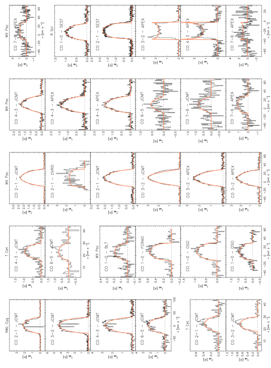
Figure 17: Profiles of $\@element[12]{\mathrm{CO}}$ with fitted soft-parabola profiles.

Fig. 17. (continued)

Fig. 17. (continued)

Fig. 17. (continued)

Fig. 17. (continued)

Fig. 17. (continued)

Fig. 17. (continued)

Fig. 17. (continued)

Fig. 17. (continued)

Fig. 17. (continued)

3

Table 11: Same as Table LABEL:tbl:12CO, for $\@element[13]{\mathrm{CO}}$-data presented in Fig. 18.

IRAS	Alternative name	$v_{\mathrm{LSR}}$	$v_{\infty}$	13 CO 2–1			13 CO 3–2			13 CO 4–3			13 CO 6–5
		km/s		$T_{\mathrm{MB,c}}$	$I_{\mathrm{MB}}$	$\beta$	$T_{\mathrm{MB,c}}$	$I_{\mathrm{MB}}$	$\beta$	$T_{\mathrm{MB,c}}$	$I_{\mathrm{MB}}$	$\beta$	$T_{\mathrm{MB,c}}$	$I_{\mathrm{MB}}$	$\beta$
-	NML Cyg	2.0	33.0	0.21	9.49	1.52	-	-	-	-	-	-	-	-	-
00192-2020	T Cet	23.0	7.0	-0.05	0.34	-	0.03	0.50	-1.47	-	-	-	-	-	-
01037+1219	WX Psc	9.0	19.8	0.36	12.93	0.07	0.48	16.01	0.48	-	-	-	-	-	-
”	”	”	”	0.23	8.09	0.11	0.34	11.39	0.21	-	-	-	-	-	-
”	”	”	”	-	-	-	0.36	11.44	0.50	-	-	-	-	-	-
01246-3248	R Scl	-17.0	17.0	-	-	-	0.11	5.17	-1.55	-	-	-	-	-	-
02168-0312	o Cet	46.4	8.1	1.39	5.22	19.70	3.13	13.35	16.91	-	-	-	5.17	26.54	11.62
03507+1115	IK Tau	33.8	18.5	0.28	10.34	-0.48	0.34	13.79	-0.68	-	-	-	-	-	-
04566+5606	TX Cam	10.8	21.2	0.10	3.72	-0.17	0.29	10.88	0.06	-	-	-	-	-	-
05073+5248	NV Aur	3.0	19.2	0.22	6.75	0.58	-	-	-	-	-	-	-	-	-
05524+0723	Alpha Ori	3.5	14.0	0.09	2.46	0.03	-	-	-	-	-	-	-	-	-
07209-2540	VY CMa	21.0	46.5	0.04	3.32	0.57	0.18	12.01	1.07	-	-	-	-	-	-
10491-2059	V Hya	-17.0	30.0	-	-	-	0.14	3.43	8.49	-	-	-	-	-	-
13269-2301	R Hya	-10.0	12.5	0.47	2.78	5.26	-	-	-	-	-	-	-	-	-
14219+2555	RX Boo	2.0	9.0	0.14	2.58	-1.32	0.57	5.51	3.04	-	-	-	-	-	-
15194-5115	II Lup	-15.0	23.0	-	-	-	0.76	31.06	-0.06	-	-	-	-	-	-
”	”	”	”	-	-	-	0.92	32.48	0.54	-	-	-	-	-	-
17411-3154	AFGL 5379	-21.2	25.0	0.16	6.05	0.84	0.05	2.70	-	-	-	-	-	-	-
18050-2213	VX Sgr	6.5	24.3	-	-	-	0.11	4.29	0.67	-	-	-	-	-	-
18059-3211	Gomez Nebula	2.7	6.0	-	-	-	0.23	1.81	3.25	-	-	-	-	-	-
18308-0503	AFGL 5502	43.0	14.7	22.97	77.97	102.80	24.38	95.37	87.94	-	-	-	-	-	-
18397+1738	IRC +20370	-0.5	16.0	-	-	-	0.28	7.41	0.76	-	-	-	-	-	-
19114+0002	V1427 Aql	99.0	40.0	-	-	-	0.43	22.20	2.12	-	-	-	-	-	-
19126-0708	W Aql	-25.0	20.0	0.14	5.03	-0.26	0.23	8.10	-0.28	-	-	-	-	-	-
”	”	”	”	-	-	-	0.25	8.68	0.49	-	-	-	-	-	-
”	”	”	”	-	-	-	0.23	7.68	0.48	-	-	-	-	-	-
19192+0922	OH 44.8-2.3	-70.5	17.7	0.10	2.56	0.13	0.08	2.04	0.49	-	-	-	-	-	-
19244+1115	IRC +10420	75.5	42.3	0.17	10.57	1.17	0.37	23.49	0.93	-	-	-	-	-	-
19486+3247	Chi Cyg	10.5	8.5	-	-	-	0.24	4.65	-0.89	-	-	-	-	-	-
20396+4757	V Cyg	15.0	15.0	0.16	3.16	0.20	-	-	-	-	-	-	-	-	-
21439-0226	EP Aqr	-33.5	11.5	0.67	3.18	208.64	1.42	6.76	136.35	0.87	3.44	16.11	-	-	-
22196-4612	pi1 Gru	-11.0	30.0	-	-	-	0.10	2.81	5.25	-	-	-	-	-	-
23166+1655	LL Peg	-31.0	16.0	-	-	-	0.86	18.36	1.62	-	-	-	-	-	-
23558+5106	R Cas	25.5	13.5	0.11	2.71	0.50	0.37	8.01	1.03	-	-	-	-	-	-

4

Table 12: References for the presented $\@element[13]{\mathrm{CO}}$ data. In case of multiple observations of a specific transition, the data are given in the exact same order as in Fig. 18. References or remarks are (1) archive data, (-) this study.

IRAS	Alternative name	13 CO 2–1		13 CO 3–2		13 CO 4–3		13 CO 6–5
		Telescope	Reference	Telescope	Reference	Telescope	Reference	Telescope	Reference
-	NML Cyg	JCMT	-	-	-	-	-	-	-
00192-2020	T Cet	JCMT	-	JCMT	-	-	-	-	-
01037+1219	WX Psc	JCMT	-	JCMT	-	-	-	-	-
”	”	JCMT	-	APEX	-	-	-	-	-
”	”	-	-	APEX	-	-	-	-	-
01246-3248	R Scl	-	-	APEX	-	-	-	-	-
02168-0312	o Cet	JCMT	-	JCMT	-	-	-	JCMT	-
03507+1115	IK Tau	JCMT	1	APEX	-	-	-	-	-
04566+5606	TX Cam	JCMT	-	JCMT	-	-	-	-	-
05073+5248	NV Aur	JCMT	-	-	-	-	-	-	-
05524+0723	Alpha Ori	JCMT	-	-	-	-	-	-	-
07209-2540	VY CMa	JCMT	-	JCMT	-	-	-	-	-
10491-2059	V Hya	-	-	APEX	-	-	-	-	-
13269-2301	R Hya	JCMT	-	-	-	-	-	-	-
14219+2555	RX Boo	JCMT	-	JCMT	-	-	-	-	-
15194-5115	II Lup	-	-	APEX	-	-	-	-	-
”	”	-	-	APEX	-	-	-	-	-
17411-3154	AFGL 5379	JCMT	-	JCMT	-	-	-	-	-
18050-2213	VX Sgr	-	-	JCMT	-	-	-	-	-
18059-3211	Gomez Nebula	-	-	JCMT	-	-	-	-	-
18308-0503	AFGL 5502	JCMT	-	JCMT	-	-	-	-	-
18397+1738	IRC +20370	-	-	APEX	-	-	-	-	-
19114+0002	V1427 Aql	-	-	APEX	-	-	-	-	-
19126-0708	W Aql	JCMT	-	APEX	-	-	-	-	-
”	”	-	-	APEX	-	-	-	-	-
”	”	-	-	APEX	-	-	-	-	-
19192+0922	OH 44.8-2.3	JCMT	-	JCMT	-	-	-	-	-
19244+1115	IRC +10420	JCMT	-	JCMT	-	-	-	-	-
19486+3247	Chi Cyg	-	-	JCMT	1	-	-	-	-
20396+4757	V Cyg	JCMT	-	-	-	-	-	-	-
21439-0226	EP Aqr	JCMT	-	JCMT	-	JCMT	-	-	-
22196-4612	pi1 Gru	-	-	APEX	-	-	-	-	-
23166+1655	LL Peg	-	-	APEX	-	-	-	-	-
23558+5106	R Cas	JCMT	-	JCMT	-	-	-	-	-

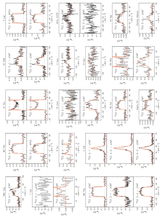
Figure 18: Profiles of $\@element[13]{\mathrm{CO}}$ with fitted soft-parabola profiles.

Fig. 18. (continued)

Appendix B Dereddening

Since the effective temperatures of late-type stars are well-determined by the intrinsic $V{\rm-}K$ colour (Sect. C.1), we need a way to derive this colour accurately. The magnitudes of both the $V$ and $K$ bands — at 0.550 $\mu$m and 2.2 $\mu$m, respectively — are reddened due to interstellar and circumstellar contributions. The data were corrected for interstellar extinction using the dust maps of Schlegel et al. (1998), which give the interstellar reddening at infinity, $E_{B-V,\infty}$, for a given set of galactic latitudes $b$ and longitudes $l$. This value was transformed into interstellar reddening at a given distance $d$ using

$$E_{B-V}=E_{B-V,\infty}\left[1-\exp{(-10\;\frac{d}{\mathrm{kpc}}\sin|b|)}\right],$$ (16)

following Feast et al. (1990). The resulting value for $E_{B-V}$ was combined with $R_{V}=3.1$ and $A_{K}=0.112\;A_{V}$ (Schlegel et al., 1998) to give interstellar extinction coefficients for the $V$ and $K$ bands.

Circumstellar extinction was not accounted for, even though it is assumed to be significant for high mass-loss rate LPV targets. Knapp et al. (1998) use the mass-loss rate $\dot{M}$ to determine the circumstellar extinction in the $K$ band. Since the aim of the paper is to establish empirical relations between stellar parameters and $\dot{M}$, this method can not be applied to the data for the sake of consistency. Knapp et al. (2003) suggest a formalism to calculate the circumstellar extinction in the $K$ band, $A_{K\mathrm{,CS}}$, as a function of $S_{12}/S_{2.2}$, the ratio of flux densities at 12 $\mu$m and 2.2 $\mu$m, respectively. This method is only valid for low optical depths (Knapp et al., 2003). When applied to the sample, unrealistic values for $A_{K\mathrm{,CS}}$ as high as several tens (LP And) or hundreds (CW Leo) of magnitudes are indeed obtained for the objects with presumed high $\dot{M}$ values. To decide, however, whether or not this correction should be applied for a given target seems arbitrary. For these reasons we did not correct for circumstellar reddening.

Appendix C Basic stellar parameters

In this appendix we describe the methods that we used to obtain the effective temperature, stellar luminosity and distance towards objects. The results are given in Table LABEL:tbl:fundamentalparameters in the paper.

C.1 Effective temperature

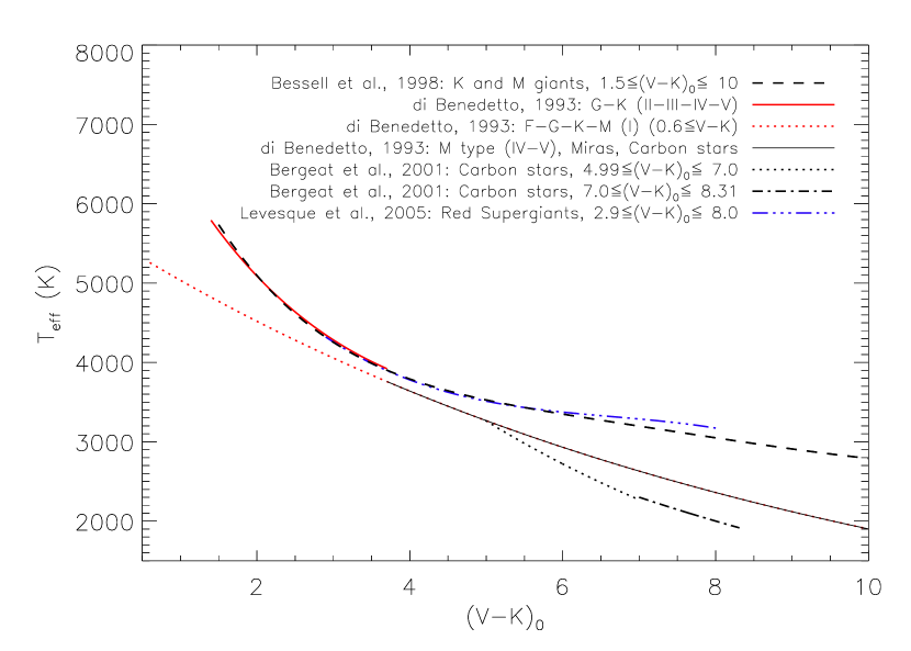
Figure 19: Different calibration relations linking the (dereddened) broad-band colour $(V{\rm-}K)_{0}$ and $T_{\mathrm{eff}}$. Relations were taken from di Benedetto (1993); Bessell et al. (1998); Bergeat et al. (2001); Levesque et al. (2005).

Since broad-band near-infrared colours are very good temperature criteria, being relatively independent of stellar gravities and abundances, they are often used to determine effective temperatures. The $V{\rm-}K$ colour is a good $T_{\mathrm{eff}}$-indicator for cool, late-type stars, e.g. GKM giants and supergiants (di Benedetto, 1993; Bessell et al., 1998; Bergeat et al., 2001; Levesque et al., 2005). For hotter A through K stars the $V-I$ colour is more suitable (Bessell et al., 1998).

In all $T_{\mathrm{eff}}$ versus $V{\rm-}K$ relations the Johnson-Cousins-Glass photometric system is used. $K$ magnitudes for the sample stars that were obtained in the systems of 2MASS ($K_{\mathrm{s}}$) and SAAO ($K_{\mathrm{SAAO}}$) were transformed via

$$K=K_{\mathrm{s}}+0.044=K_{\mathrm{SAAO}}-0.0275.$$ (17)

following (Bessell, 2005). Since the accuracy of the $K_{\mathrm{SAAO}}$-measurements ($\sim$0.03 mag; Olivier et al., 2001) is almost a factor 10 better than that of $K_{\mathrm{s}}$-data ($\sim$0.2 mag), preference was given to the SAAO-measurements when both were available. The errors on the magnitudes are expected to be small relative to the amplitude in the $K$ band caused by pulsations of the stars. The error bars on the $T_{\mathrm{eff}}$ values determined here, were calculated assuming an error on $(V{\rm-}K)_{0}$ of 1 mag, leading to rather conservative temperature estimates.

In all equations listed $(V{\rm-}K)_{0}$ is the intrinsic $V{\rm-}K$ broad-band colour with (1) both the $V$ and $K$ magnitudes at maximum light, or (2) both at their mean value if maximum light was not available, and (3) corrected for interstellar reddening in the way described in Sect. B.

C.1.1 Long-period variables: Miras, semi-regulars and irregular variables

Bessell et al. (1998) defined a $T_{\mathrm{eff}}$ versus $V{\rm-}K$ calibration for KM giants (luminosity class III), given by

$$T_{\mathrm{eff}} = 9037.597-3101.282\times(V{\rm-}K)_{0}$$

$$+717.7044\times(V{\rm-}K)_{0}^{2}$$

$$-85.83809\times(V{\rm-}K)_{0}^{3}$$

$$+5.021194\times(V{\rm-}K)_{0}^{4}$$

$$-0.1137841\times(V{\rm-}K)_{0}^{5}.$$

This relation is valid for 1.5 mag$\,\leq(V{\rm-}K)_{0}\leq\,$10 mag (see Fig. 19). However, Bessell et al. (1998) mention that their static model atmospheres cannot adequately represent the M giants cooler than 3000 K, since most of these are long-period variables (LPVs) with shock waves traversing and greatly extending their atmospheres.

di Benedetto (1993) presented a temperature calibration in which $T_{\mathrm{eff}}$ is derived from angular-diameter measurements based on Michelson interferometry. In case of variable stars, measurements at maximum light were used. The effective temperature of GK stars of luminosity classes II-III-IV-V is described by

$$\log T_{\mathrm{eff}} = a-(b+0.0118)(V{\rm-}K)_{0}$$

$$+0.0118(V{\rm-}K)_{0}^{2}$$

for 1.4 mag$\,\leq(V{\rm-}K)_{0}\leq\,$3.7 mag, for FGKM supergiants by

$$\log T_{\mathrm{eff}}=(a-0.205)-(b-0.086)(V{\rm-}K)_{0}$$ (20)

for $(V{\rm-}K)_{0}\geq 0.6$ mag and for M-type giants of type IV, Miras and carbon stars by Eq. 20 for 3.7 mag$\,\leq(V{\rm-}K)_{0}\leq\,$10 mag (see Fig. 19). The constants $a$ and $b$ in Eqs. C.1.1 and 20, and the validity ranges in terms of $(V{\rm-}K)_{0}$ are listed in Table 14.

For oxygen-rich LPVs, except for OH/IR stars, the effective temperature was derived via Eq. 20 (di Benedetto, 1993). The uncertainty on the temperature would then be of the order of 1 % according to di Benedetto (1993).

Bergeat et al. (2001) focussed on carbon-rich objects and derived a relation for $T_{\mathrm{eff}}$ versus $V{\rm-}K$ given by Eqs. C.1.1, C.1.1 and 23. The notation $T_{\mathrm{eff,d}}$ denotes that the relation is based on angular-diameter measurements, $T_{\mathrm{eff}}$ is the final temperature adopted for their sample stars.

$$\log T_{\mathrm{eff,d}} = -0.079_{(\pm 0.008)}(V{\rm-}K)_{0}+3.91_{(\pm 0.02)}$$

$$\qquad\qquad\qquad\qquad{\rm for}\;4.99\leq(V{\rm-}K)_{0}\leq 7$$

$$\log T_{\mathrm{eff,d}} = -0.061_{(\pm 0.008)}(V{\rm-}K)_{0}+3.79_{(\pm 0.02)}$$

$$\qquad\qquad\qquad\qquad{\rm for}\;7\leq(V{\rm-}K)_{0}\leq 8.31$$

$$\log T_{\mathrm{eff,d}} = 1.003\log T_{\mathrm{eff}}-0.009$$ (23)

These $T_{\mathrm{eff}}$ values are estimated to be accurate to within an error margin of $\pm 140$ K (Bergeat et al., 2001). Because this $T_{\mathrm{eff}}$-calibration is based on a sample of 54 carbon-rich stars, preference was given to this calibration, rather than to the one by di Benedetto (1993), in case of carbon stars. The validity range was adopted to be $4.99\,\leq(V{\rm-}K)_{0}\leq\,$8.31 mag, consistent with the minimum and maximum in Table 5 of Bergeat et al. (2001).

It is clearly visible from Fig. 19 that the carbon stars have lower predicted effective temperatures than the oxygen-rich stars. This is in agreement with the results of Marigo (2002), showing a clear dichotomy in $T_{\mathrm{eff}}$ between both chemical types of AGB stars. This dichotomy is caused by different molecular opacities in stellar atmospheres with differing C/O abundance ratios.

When using these $T_{\mathrm{eff}}$ estimators, one should be aware of the effect of circumstellar reddening on the $V$ and $K$ band data. This reddening is stronger for objects with higher values of $\dot{M}$ and depends on the chemistry of the central star (Knapp et al., 1998, 2003). As mentioned in Appendix B, the data were not corrected for circumstellar reddening.

For oxygen-rich targets with $(V{\rm-}K)_{0}$ outside the valid ranges for the above mentioned relations, the temperature corresponding to the spectral type listed in Table LABEL:tbl:fundamentalparameters was used (Table 13; Marigo et al., 2008). An error bar of 500 K was assumed for these values. For the carbon-rich targets with $(V{\rm-}K)_{0}$ outside the valid ranges the effective temperatures found in literature were used. References are given in Table LABEL:tbl:fundamentalparameters.

Table 13: Effective temperature $T_{\mathrm{eff}}$ versus spectral type for oxygen-rich targets as given by Marigo et al. (2008). They are used in this paper in case of oxygen-rich LPVs which have their dereddened $(V{\rm-}K)_{0}$ broad-band colour outside the valid ranges for the listed $T_{\mathrm{eff}}$ versus $(V{\rm-}K)_{0}$ relations.

Spectral Type	M0	M1	M2	M3	M4	M5
$T_{\mathrm{eff}}$ (K)	3850	3750	3650	3550	3490	3397
Spectral Type	M6	M7	M8	M9	M10
$T_{\mathrm{eff}}$ (K)	3297	3129	2890	2667	2500

Table 14: Coefficients $a$ and $b$ for the $T_{\mathrm{eff}}$ calibration from $V{\rm-}K$ colours via Eqs. C.1.1 and 20. Taken from di Benedetto (1993).

Spectral type	Luminosity class	$(V{\rm-}K)_{0}$	$a$	$b$
G-K	II-III-IV-V	$1.4-3.7$	3.927	0.122
M	III	$3.7-10$	3.833	0.101
M	II	$3.7-10$	3.859	0.108
F-G-K-M	I	$0.6-10$	3.954	0.133
M	IV-V	$3.7-10$	3.954	0.133
M	Mira	$3.7-10$	3.954	0.133
C	Carbon star	$3.7-10$	3.954	0.133

C.1.2 OH/IR stars

In the case of OH/IR stars the photosphere is not easily probed since the CSE is optically thick and consequently the infrared sources often do not have optical counterparts. Therefore, the $V{\rm-}K$ colour is no longer a meaningful diagnostic of $T_{\mathrm{eff}}$. For these objects an effective temperature of $2750\pm 750$ K was assumed.

C.1.3 Red supergiants

The $T_{\mathrm{eff}}$-calibration of Bessell et al. (1998) is not valid for red supergiants (RSGs) because of their low $\log g$-values. Levesque et al. (2005) derived a $T_{\mathrm{eff}}$-scale for RSGs in the Milky Way given by Eq. C.1.3. This relation between the broad-band colour $V{\rm-}K$ and the effective temperature is consistent with the results from their grid of marcs models and is valid for $2.9{\rm\,mag}\leq(V{\rm-}K)_{0}\leq 8.0{\rm\,mag}$. Adopting this new $T_{\mathrm{eff}}$-calibration for RSGs yields a better agreement between evolutionary tracks and observationally determined locations of RSGs in the HR-diagram (see Massey et al., 2008, Fig. 3). This $T_{\mathrm{eff}}$-scale for RSGs closely follows the relation of Bessell et al. (1998) defined for KM giants (see Fig. 19), but since Eq. C.1.3 was derived especially for RSGs, preference was given to this relation over Eq. C.1.1. It is given by

$$T_{\mathrm{eff}} = 7741.9-1831.83(V{\rm-}K)_{0}$$

$$+263.135(V{\rm-}K)_{0}^{2}-13.1943(V{\rm-}K)_{0}^{3}.$$

Levesque et al. (2005) expect that the effective temperatures for M-type supergiants were obtained with a precision of 50 K.

For RSGs with $(V{\rm-}K)_{0}<2.9$ or $(V{\rm-}K)_{0}>8.0$, the temperature was determined using the scale of $T_{\mathrm{eff}}$ versus spectral type — in case of galactic targets — presented by Levesque et al. (2005).

C.1.4 Yellow hypergiants

The adopted $T_{\mathrm{eff}}$-calibration of di Benedetto (1993) for FGKM targets of luminosity class I seems in accordance with the results presented by de Jager (1998) and Oudmaijer et al. (2008) for the yellow hypergiants (YHGs) IRC +10420 and AFGL 2343. Since both objects are known to exhibit large $T_{\mathrm{eff}}$-variations on time scales of a few decades (Oudmaijer et al., 2008), this calibration is somewhat uncertain.

C.1.5 Alternative methods

Haniff et al. (1995) derive effective temperatures from angular diameters and bolometric fluxes obtained through fits to optical and infrared photometry. The infrared flux method (IRFM), presented by Blackwell & Shallis (1977), consists of determining the ratio of the bolometric flux to the flux in a selected photometric band and comparing these results to predictions from model atmospheres. Since the goal of this paper is not to individually model all sample targets, we did not pursue these methods, nor did we perform full fits of the spectral energy distributions (SEDs). The latter would require detailed radiative transfer analysis for each star.

C.2 Luminosity

The luminosities of Miras, OH/IR stars, semi-regular pulsators of types a and b and red supergiants were determined through empirical period-bolometric magnitude relations presented in the literature (Feast et al., 1989; Groenewegen & Whitelock, 1996; Whitelock et al., 1991; Barthès et al., 1999; Whitelock & Feast, 2000; Yeşilyaprak & Aslan, 2004). These relations are then used to calculate luminosities adopting the solar bolometric magnitude $M_{\mathrm{bol},\odot}$ $=4.75$ mag.

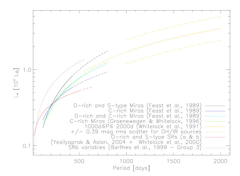
Figure 20: $P-$$L_{\star}$ relations taken from Groenewegen & Whitelock (1996); Feast et al. (1989); Whitelock et al. (1991); Yeşilyaprak & Aslan (2004); Barthès et al. (1999), and Whitelock et al. (2000). Dashed lines indicate extrapolations of the $P-$$L_{\star}$ relations from the literature to shorter or longer periods of pulsation. See text for details.

C.2.1 Miras and OH/IR stars

Feast et al. (1989) derived period-luminosity, $P-$$L_{\star}$, relations for oxygen-rich and carbon-rich Miras in the LMC with periods ranging from 115 up to 420 days. Groenewegen & Whitelock (1996) revised the $P-$$L_{\star}$ relation for carbon-rich Miras and extended the period range up to periods of 520 days. Whitelock et al. (1991) developed a similar relation for OH/IR targets with periods of pulsation exceeding 1000 days. These relations - and their extrapolations to shorter or longer pulsation periods - are shown in Fig. 20.

The relation derived by Feast et al. (1989) for oxygen-rich Miras was assumed to be valid also for galactic oxygen-rich Miras and was adjusted with a distance modulus of 18.5 mag. It is given by

$$M_{\mathrm{bol,O-MIRA,OH/IR}}=-3.00_{\pm 0.24}\log P+2.85_{\pm 0.57},$$ (25)

with $P$ in days.

Whitelock et al. (1991) mention a rather large scatter of 0.39 mag on their derived $P-$$L_{\star}$ relation for OH/IR variables with periods ranging up to 2000 days. The large range in predicted luminosities associated with this scatter has been made visible in the figure. Note that the extrapolated relation for oxygen-rich Miras derived by Feast et al. (1989) matches the higher luminosity edge derived for OH/IR targets very well. Whitelock et al. (1991) also point out that there are suggestions that the luminosities of OH/IR sources with $P>1000$ days probably follow this extrapolated $P-$$L_{\star}$ relation that was established for oxygen-rich Miras by Feast et al. (1989). Because of these arguments and the strong evolutionary connection between oxygen-rich Miras and OH/IR stars (see Sect. 2.1) we adopt the $P-$$L_{\star}$ relation of Feast et al. (1989) for oxygen-rich Miras, given in Eq. 25, for the determination of luminosities for all oxygen-rich Miras and OH/IR targets, regardless of their period of pulsation. Relation 25 was also used in determining the luminosity of S-type Miras in the sample.

Luminosities of carbon-rich Miras were determined via

$$M_{\mathrm{bol,C-MIRA}}=-2.59\log P+2.02_{(\pm 0.26)}$$ (26)

following Groenewegen & Whitelock (1996). This relation predicts luminosities substantially higher than does the relation derived by Feast et al. (1989). Preference was given to the former since the sample of Groenewegen & Whitelock (1996) is almost three times as large as the one used by Feast et al. (1989) (54 versus 20 objects). For longer-period carbon-rich Miras, this $P-$$L_{\star}$ relation was extrapolated, similar to what was done in the oxygen-rich case.

C.2.2 Semi-regular pulsators: SRa & SRb

Many semi-regular type a (SRa) objects differ from Miras only by their smaller amplitudes in the $V$ band ($\Delta V<2.5$ mag). Objects classified as semi-regular b (SRb) variables have rather poorly defined periodicity, show a superposition of multiple pulsation periods, or have alternating intervals of periodic and slow irregular changes.

Semi-regulars and Miras are linked in terms of evolution, since SRs of types a and b are thought to be the progenitors of Miras (Whitelock & Feast, 2000; Yeşilyaprak & Aslan, 2004). Therefore some type of $P-$$L_{\star}$ relation, analogous to those for Miras is probably justified for these LPVs.

Yeşilyaprak & Aslan (2004) presented period-magnitude relations for all magnitudes in the Johnson system and the IRAS system for SRa and SRb stars. To determine the bolometric magnitude, and hence the luminosity, only the $J$ and $K$ period – magnitude relations were used.

$$J = -1.03_{(\pm 0.56)}\log P-3.47_{(\pm 0.98)}$$ (27)

$$K = -1.38_{(\pm 0.58)}\log P-3.99_{(\pm 1.00)}$$ (28)

Yeşilyaprak & Aslan mention a scatter of 0.63 mag and 0.85 mag for the $J$ and $K$ relations, respectively. The bolometric correction on the $K$ magnitude was calculated via

$$BC_{K} = 10.86-38.10(J-K)_{0}$$

$$+64.16(J-K)_{0}^{2}-50.72(J-K)_{0}^{3}$$

$$+19.48(J-K)_{0}^{4}-2.94(J-K)_{0}^{5}$$

taken from Whitelock et al. (2000), where

$$M_{\mathrm{bol}} = K+BC_{K}.$$ (30)

Relations 27 and 28 were however only adopted in estimating the luminosities for SRa variables, and not for the SRb variables in the sample. Barthès et al. (1999) presented $P-(J-K)$ relations for long-period variables, including a large number of SRb type stars. The sample of Barthès et al. (1999) is divided in four groups, and the SRb type stars are largely split up in two of those — Groups 2 and 3, corresponding to younger and older kinematic properties respectively. Their Group 2 is far less luminous than their Group 3 and preference is given to the relations for their Group 3 - Eqs. 31 and 32 - since these estimates are in best accordance with luminosities derived in the literature for the SRb objects in the sample. Bolometric corrections were again derived via Eq. C.2.2.

$$K_{\mathrm{SRb}} = -2.11_{(\pm 0.13)}(\log P-1.75)-6.51_{(\pm 0.05)}$$ (31)

$$(J-K)_{0} = 0.17_{(\pm 0.04)}\log P+0.85_{(\pm 0.08)}$$ (32)

The uncertainties on calculated luminosities only take into account the uncertainties on the coefficients in Eqs. 25 through 32. The error bars on the pulsation periods are assumed to be small compared to the errors on the coefficients in the above relations.

C.2.3 Red supergiants

The luminosity of the RSGs in the sample was determined as a function of period of pulsation and effective temperature. Eq. 33 gives the relation between the $K$ magnitude and the pulsation period for RSGs in the milky way galaxy as presented by Dambis (1993). This relation was completed with the bolometric correction on the $K$ band magnitudes given by Levesque et al. (2005) (Eq. 34). This method leads to luminosities ranging from $\sim$$10^{4}$ L_⊙ up to $\sim$$5\;10^{5}$ L_⊙. It is given by

$$K = -10.10_{(\pm 0.08)}-3.44(\log P-2.7)$$ (33)

$$BC_{K} = 5.574-0.7589\times\frac{T_{\mathrm{eff}}}{1000\;\mathrm{K}}$$ (34)

C.2.4 Yellow hypergiants

No general period-luminosity relations can be established for these targets because of their very strong variability. The latter is reflected in the multiple motions from blue to red and vice versa in the HR diagram (de Jager, 1998; Oudmaijer et al., 2008). For both AFGL 2343 and IRC +10420, the two YHGs in the sample, luminosities were taken from de Jager (1998), yielding values for $\log L_{\star}/L_{\odot}$ of 5.30 and 5.80, respectively.

C.2.5 Alternative methods

More recently, Barthès et al. (1999) and Knapp et al. (2003) derived $P-K$ relations for oxygen-rich LPVs, including Miras and semi-regulars of types a and b. Using these relations in determining the luminosities of Miras would introduce extra uncertainties, since bolometric corrections for $K$ band magnitudes would have to be derived. This is the main reason why the above mentioned $P-$$M_{\mathrm{bol}}$ relations of Feast et al. (1989) and Groenewegen & Whitelock (1996) were used for Miras.

C.3 Distance

Distances towards the sample stars have been determined in various ways. (1) OH-maser phase lag distances were used for most OH/IR stars, since these provide a very accurate distance estimate (van Langevelde et al., 1990). (2) Hipparcos-data were used when available with a relative error lower than 50 %. (3) values in the literature derived from SED fitting were used and assumed to have uncertainties of 50 %, unless stated otherwise in the original papers.

C.3.1 Alternative method

An alternative method to derive distances is to compare observed magnitudes with absolute magnitudes predicted through formalisms as presented in Sect. C.2. The relations that could be used for distance determination from magnitudes for Miras are

$$K_{\mathrm{O-MIRA}} = -3.47_{(\pm 0.19)}\log P+0.98_{(\pm 0.45)}$$ (35)

$$K_{\mathrm{C-MIRA}} = -3.56\log P+1.14$$ (36)

Since the $K$ magnitude is less sensitive to metallicity than the bolometric magnitude $m_{\rm bol}$, it is a better distance indicator (Whitelock & Feast, 2000, and references therein). The strong variability in the $K$ band of most sample stars, however, gives rise to large uncertainties on absolute magnitudes. An additional constraint to the application of this method to determine distances is that the circumstellar material can redden the $K$ band magnitudes significantly.