A loop of $SU(2)$ gauge fields
stable under the Yang-Mills flow

Daniel Friedan

Department of Physics and Astronomy

Rutgers, The State University of New Jersey

Piscataway, New Jersey 08854-8019 USA

and

Natural Science Institute

The University of Iceland

Reykjavik, Iceland

friedan@physics.rutgers.edu

The gradient flow of the Yang-Mills action acts pointwise on closed loops of gauge fields. We construct a topologically nontrivial loop of $SU(2)$ gauge fields on $S^{4}$ that is locally stable under the flow. The stable loop is written explicitly as a path between two gauge fields equivalent under a topologically nontrivial $SU(2)$ gauge transformation. Local stability is demonstrated by calculating the flow equations to leading order in perturbations of the loop. The stable loop might play a role in physics as a classical winding mode of the lambda model, a 2-d quantum field theory that was proposed as a mechanism for generating spacetime quantum field theory. We also present evidence for 2-manifolds of $SU(3)$ and $SU(2)$ gauge fields that are stable under the Yang-Mills flow. These might provide 2-d instanton corrections in the lambda model.

For Isidore M. Singer in celebration of his eighty-fifth birthday.

1 Introduction

We are interested in the long time behavior of the Yang-Mills flow acting on topologically nontrivial loops and 2-spheres of $SU(2)$ and $SU(3)$ gauge fields on $S^{4}$. Singer [1] noted that the homotopy groups $\pi_{n}(\mathcal{A}/\mathcal{G})$ of the space $\mathcal{A}/\mathcal{G}$ of gauge fields on $S^{4}$ modulo gauge equivalence are given by the homotopy groups of the gauge group $G$,

$$\pi_{n}(\mathcal{A}/\mathcal{G})=\pi_{n-1}\mathcal{G}=\pi_{n+3}G\,.$$ (1)

There are nontrivial loops of $SU(2)$ gauge fields becausen $\pi_{4}SU(2)=\mathbb{Z}_{2}$ [2, 3]. For $SU(3)$, there are no nontrivial loops because $\pi_{4}SU(3)=0$ [4]. There are topologically nontrivial 2-spheres of gauge fields for both $SU(2)$ and $SU(3)$ because $\pi_{5}SU(3)=\mathbb{Z}$ [4] and $\pi_{5}SU(2)=\mathbb{Z}_{2}$ [5, 6].

Our motivation is a hypothetical effect in a speculative theory of physics. The lambda model [7] is a 2-dimensional nonlinear model whose target space is the manifold of spacetime fields. The short distance fluctuations in a 2-d nonlinear model generate a measure on its target manifold, called the a priori measure. In the lambda model, the a priori measure is a measure on the manifold of spacetime fields: a quantum field theory. The a priori measure of the lambda model is generated by a diffusion process in the loop space of the target manifold, driven by the gradient flow of the classical spacetime action. We are pursuing the possibility that the quantum field theory generated by the lambda model will be different from the canonically quantized field theory because of nonperturbative 2-dimensional effects. The dominant nonpertubative effects at weak coupling will be due to winding modes, which are associated with topologically nontrivial loops in the target manifold, and instantons, which are associated with topologically nontrivial 2-spheres in the target manifold. Winding modes in the lambda model might give rise to non-canonical physical states in the spacetime quantum field theory. Instantons in the lambda model might produce non-canonical interactions.

We are motivated by these possibilities to investigate the concentration points of the gradient flow of the Yang-Mills action as it acts on loops and on 2-spheres of $SU(2)$ and $SU(3)$ gauge fields on $\mathbb{R}^{4}$. We replace $\mathbb{R}^{4}$ by its conformal compactification $S^{4}$, studying gauge fields in topologically trivial bundles over $S^{4}$. As it turns out, our results will be applicable to gauge fields on $\mathbb{R}^{4}$ because they will concern fixed points of the Yang-Mills flow, i.e., critical points of the Yang-Mills action, which is conformally invariant.

We find that the Yang-Mills flow concentrates on a nontrivial loop of singular $SU(2)$ gauge fields made out of a zero-size instanton and a zero-size anti-instanton. We find evidence that the Yang-Mills flow concentrates on a nontrivial 2-sphere of singular $SU(3)$ gauge fields also made from a zero-size instanton and a zero-size anti-instanton. We find evidence that the flow concentrates on a nontrivial 2-sphere of $SU(2)$ gauge fields made from configurations of two zero-size instantons and two zero-size anti-instantons. These singular gauge fields live in the boundary of the manifold of gauge fields.

The natural metric on the manifold of gauge fields degenerates at the boundary, so the stable loop of gauge fields has zero length and the presumptive stable 2-spheres have zero area. This keeps alive the hope that they might have observable effects at low energy in the quantum field theory. Loops or 2-spheres of nonsingular gauge fields, with nonzero length or area, would make contributions in the lambda model only visible at extreme small distance in spacetime.

Let ${\mathcal{A}}$ be the space of connections (gauge fields) in the trivial $SU(2)$ principle bundle over $S^{4}$. A connection is described by its corresponding covariant derivative $D=d+A$, where $A$ is an $su(2)$-valued 1-form on $S^{4}$. The curvature 2-form is

$$F=D^{2}=dA+A^{2}\,.$$ (2)

The group of gauge transformations, $\mathcal{G}$, is the group of maps $\phi:S^{4}\rightarrow SU(2)$ acting on connections by

$$d+A\mapsto\phi(d+A)\phi^{-1}\qquad A\mapsto\phi d(\phi^{-1})+\phi A\phi^{-1}\,.$$ (3)

${\mathcal{A}}/\mathcal{G}$ is the space of gauge equivalence classes of connections.

The Yang-Mills (Y-M) action is

$$S_{\mathit{YM}}(A)=\frac{1}{8\pi^{2}}\int_{S^{4}}\mathrm{tr}(-F*F)$$ (4)

where ${*}$ is the Hodge operator, which takes $k$-forms to $(4-k)$-forms and satisfies ${*}^{2}=(-1)^{k}$. The action $S_{\mathit{YM}}$ is normalized so that the BPST instanton [8] has action $1$. The Yang-Mills flow on the space of connections is the gradient flow of the Y-M action [9, 10, 11, 12, 13],

$$\frac{dA\hfil}{dt}=-\nabla S_{\mathit{YM}}=*\,D*F=*\,\left(d*F+[A,\,*F]\right)\,.$$ (5)

The sign is such that $S_{\mathit{YM}}$ decreases along the flow. The gradient is taken with respect to the $L_{2}$ metric on variations $\delta A$ of $A$,

$$(ds)^{2}_{\mathcal{A}}=\frac{1}{4\pi^{2}}\int_{S^{4}}\mathrm{tr}(-\delta A*\delta A)\,.$$ (6)

The Y-M flow is gauge invariant (commutes with gauge transformations), so it acts on the gauge equivalence classes ${\mathcal{A}}/\mathcal{G}$.

The Y-M flow acts pointwise on parametrized loops in $\mathcal{A}/\mathcal{G}$, acting simultaneously on each connection along the loop. This action on parametrized loops is invariant under reparametrizations of the loop, so the Y-M flow acts on the unparametrized loops $\mathit{Maps}(S^{1}\rightarrow\mathcal{A}/\mathcal{G})/\mathit{Diff}(S^{1})$. We are interested in the long time behavior of the Y-M flow acting on the unparametrized loops in $\mathcal{A}/\mathcal{G}$. We expect that each connected component of the loop space contains a stable loop that is the generic attractor for the Y-M flow. There is an obvious stable attractor among the topologically trivial loops: the constant loop at the flat connection. All nearby connections are driven to the flat connection, so all nearby loops are driven to the constant loop.

The connected components of the loop space are the elements of the fundamental group $\pi_{1}({\mathcal{A}}/\mathcal{G})$. As Singer [1] pointed out, the long exact sequence of homotopy groups implies $\pi_{n}({\mathcal{A}}/\mathcal{G})=\pi_{n-1}\mathcal{G}$, since $\mathcal{A}$ is a contractible space. In particular,

$$\pi_{1}({\mathcal{A}}/\mathcal{G})=\pi_{0}\mathcal{G}=\pi_{4}SU(2)=\mathbb{Z}_{2}\,.$$ (7)

The loop space of $\mathcal{A}/\mathcal{G}$ thus has two connected components: the trivial (contractible) loops and the nontrivial (non-contractible) loops. The nontrivial loops in ${\mathcal{A}}/\mathcal{G}$ lift to paths in $\mathcal{A}$ whose endpoints are gauge equivalent under a nontrivial gauge transformation, i.e., one that belongs to the nontrivial connected component of $\mathcal{G}$.

Heuristically, we expect a stable nontrivial loop to be associated with an index 1 fixed point — a fixed point whose unstable manifold is one-dimensional. The unstable manifold will consist of two outgoing branches. We expect each of the two branches to flow to a flat connection, the two flat connections being gauge equivalent under a nontrivial gauge transformation. The unstable manifold will thus form a nontrivial loop in $\mathcal{A}/\mathcal{G}$. This loop will be locally stable because any nearby loop will intersect the codimension 1 stable manifold of the fixed point.

Here, we use elementary methods to find a locally stable attractor among the nontrivial loops. We start out completely ignorant of the long time fate of a generic nontrivial loop of connections under the Y-M flow. In hope of relieving our ignorance, we pick a particular nontrivial loop of connections, derived from the homogeneous space $SU(3)/SU(2)=S^{5}$, then try by numerical calculation to discover its long time behavior under the Y-M flow. The numerical results suggest the existence of an index 1 fixed point lying within the space of singular connections that consist of a zero-size instanton at one point and a zero-size anti-instanton at a second point and are flat everywhere else. A nontrivial loop of such singular connections is written explicitly. The loop is parametrized by the angle $\sigma$ that measures the relative rotation between the instanton and the anti-instanton. The Y-M flow is calculated asymptotically near these twisted pairs. The stable loop of twisted pairs is found by examining the flow lines.

Sibner, Sibner and Uhlenbeck [14] study a related problem. They consider the submanifold $(\mathcal{A}/\mathcal{G})_{\mathit{inv}}\subset\mathcal{A}/\mathcal{G}$ consisting of the $SU(2)$ connections on $S^{4}$ invariant under a certain $U(1)$ symmetry group. The submanifold $(\mathcal{A}/\mathcal{G})_{\mathit{inv}}$ separates into a series of connected components, indexed by $m\geq 1$. Each connected component has nontrivial $\pi_{1}$. For each $m$, they write a nontrivial loop consisting of a zero-size $m$-instanton at one pole in $S^{4}$ glued to a zero-size $m$-anti-instanton at the other pole. For $m=1$, their loop is exactly the loop of twisted pairs considered here. They point to [15] for references on the nontriviality of such loops. They apply a min-max procedure: minimizing the maximum value of $S_{\mathit{YM}}$ along the loop, over all nontrivial loops in $(\mathcal{A}/\mathcal{G})_{\mathit{inv}}$ that belong to the same homotopy class. For $m\geq 2$, they are able to make a small perturbation of the loop of singular connections to obtain a loop of nonsingular connections that has $S_{\mathit{YM}}<2m$ everywhere on the loop. They then prove that the min-max connection provides a non-singular critical point of the Y-M action that is neither self-dual nor anti-self-dual — the first examples of such in 4 dimensions. Their min-max connections should have index 1 within the submanifold $(\mathcal{A}/\mathcal{G})_{\mathit{inv}}$ and should correspond to globally stable loops under the Y-M flow acting on $(\mathcal{A}/\mathcal{G})_{\mathit{inv}}$. Here, we treat a much more elementary question: the local stability of the loop of twisted pairs (their $m=1$ loop) within the full $\mathcal{A}/\mathcal{G}$.

We present a summary of our results on the stable loop of $SU(2)$ gauge fields, then some preliminaries on notation and basic formulas, then the computer calculation, then the explicit loop of twisted pairs and its nontriviality, then the calculation of the flow asymptotically nearby and the demonstration of local stability. We present evidence of stable 2-manifolds for the gauge groups $SU(3)$ and $SU(2)$. For $SU(3)$ we expect this to be a stable 2-sphere. For $SU(2)$ we expect either a 2-torus or 2-sphere. At the end, we raise some mathematical questions and make some very preliminary remarks about possible effects in the lambda model.

2 Summary of the result

2.1 BPST instantons

The BPST instanton [8] is the self-dual gauge field, ${*}F=F$, in the $SU(2)$ bundle of Pontryagin index ${+}1$ over $S^{4}$. The anti-instanton is the anti-self-dual gauge field, ${*}F=-F$, in the bundle of Pontryagin index $-1$. Explicit formulas are given in section 3.13 below. The instantons are parametrized by a point in $S^{4}$ — the location of the instanton — and by a nonnegative real number — the size of the instanton — and by an element in $SU(2)/\{\pm\mathbf{1}\}$ — the orientation of the instanton. Strictly speaking, all the orientations of an isolated instanton are gauge equivalent. The orientation becomes significant when instantons are combined, the relative orientations being gauge invariant.

In the limit where the size of the instanton goes to $0$, the instanton becomes a singular connection whose action density $({8\pi^{2}})^{-1}\mathrm{tr}(-F*F)$ is a Dirac delta-function concentrated at the location of the instanton, while $F=0$ everywhere else.

2.2 Twisted pairs

A twisted pair is a singular gauge field in the trivial bundle consisting of a zero-size instanton at one point in $S^{4}$ and a zero-size anti-instanton at a second point. The zero size limit is taken with the ratio of the sizes held fixed. A twisted pair is everywhere either self-dual or anti-self-dual or flat, so each twisted pair is a fixed point of the flow. The twisted pairs are parametrized by the location $x_{+}\in S^{4}$ of the instanton, by the location $x_{-}\in S^{4}$ of the anti-instanton, by the ratio $\rho_{+}/\rho_{-}$ of the size of the instanton to the size of the anti-instanton, and by the relative orientation or twist, $g_{\mathit{tw}}\in SU(2)/\{\pm 1\}$. Of the two orientations, the instanton’s and the anti-instanton’s, one is eliminated by a gauge transformation, leaving only the relative orientation to parametrize the twisted pairs. We establish by an explicit calculation that a loop of twisted pairs is nontrivial in $\mathcal{A}/\mathcal{G}$ if $g_{\mathit{tw}}$ traverses a nontrivial loop in the space $SU(2)/\{\pm 1\}$ of relative orientations.

2.3 Conformal symmetry

The Hodge ${*}$-operator acting on 2-forms is conformally invariant in four dimensions, so the conformal symmetry group of $S^{4}$, which is $SO(1,5)$, acts on the space of critical points of the Yang-Mills action, in particular on the space of twisted pairs. Using conformal transformations, we can move the zero-size instanton to the south pole in $S^{4}$ and the zero-size anti-instanton to the north pole. We can make the sizes of the instanton and the anti-instanton equal. The remaining subgroup of the conformal group is $SO(4)$, which acts on the twist $g_{\mathit{tw}}\in SU(2)/\{\pm\mathbf{1}\}$ by conjugations. So we can diagonalize $g_{\mathit{tw}}$. The twisted pair is invariant under the remaining $U(2)$ subgroup of $SO(4)$. The conformal equivalence classes of twisted pairs form a one parameter family labelled by the conjugacy classes of $SU(2)/\{\pm\mathbf{1}\}$. Each twisted pair has a $U(2)$ symmetry.

The metric on $\mathcal{A}$ is not conformally invariant, so the Y-M flow is not conformally invariant away from the fixed points. Near the fixed points, the conformal group acts merely by rescaling parameters, so the qualitative behavior of the flow in the neighborhood of the fixed points is conformally invariant. It is enough to study the Y-M flow near a slice of the conformal equivalence classes, consisting of a representative in each conformal equivalence class of twisted pairs.

2.4 The Y-M flow near the twisted pairs

Instantons and anti-instantons are individually stable under the Y-M flow, so the Y-M flow very near the twisted pairs reduces to a flow in a slow manifold parametrized by an asymptotically small instanton and an asymptotically small anti-instanton.

We represent the conformal equivalence classes by puting the instanton at the south pole and the anti-instanton at the north pole, by making their sizes equal, $\rho_{+}=\rho_{-}=\rho\approx 0$, and by diagonalizing the twist,

$$g_{\mathit{tw}}=\begin{pmatrix}e^{\frac{1}{2}i\sigma}&0\\ 0&e^{-\frac{1}{2}i\sigma}\end{pmatrix}\,,\qquad\sigma\in[0,2\pi]\,.$$ (8)

The slow manifold is represented by a two dimensional space of connections parametrized by $\rho\approx 0$ and by $\sigma$. The twisted pairs are at $\rho=0$.

We calculate the Y-M flow equations to leading order in $\rho$,

$$\frac{d\rho}{dt}=\rho^{3}(1+2\cos\sigma)+O(\rho^{5})\,,\qquad\frac{d\sigma}{dt}=-8\rho^{2}\sin\sigma+O(\rho^{4})\,.$$ (9)

The flow lines follow the curves

$$\rho^{8}(1-\cos\sigma)\sin\sigma=C\,.$$ (10)

as pictured in Figure 1.

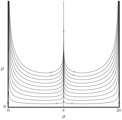
Figure 1: The flow on the slow manifold. The twisted pairs are represented by the horizontal axis. The vertical axes at $\sigma=0$ and $\sigma=2\pi$ are identified under a nontrivial gauge transformation.

The twisted pairs lie on the horizontal axis, $\rho=0$. The vertical axes at $\sigma=0$ and at $\sigma=2\pi$ are identified by a nontrivial gauge transformation $\phi:S^{4}\rightarrow SU(2)$. The maximally twisted pairs are those with $\mathrm{tr}(g_{\mathit{tw}})=0$, represented in Figure 1 by the point $\sigma=\pi$ on the horizontal axis. The attracting (stable) manifold of the maximally twisted pairs is represented in Figure 1 by the vertical line $\sigma=\pi$. It has codimension 1 in $\mathcal{A}/\mathcal{G}$. If a loop of connections intersects it, the Y-M flow drives the intersection point to a maximally twisted pair. An infinitesimal neighborhood within the loop around the intersection point is driven to the unstable manifold of that maximally twisted pair, which is represented in Figure 1 by the three axes: the horizontal axis $\rho=0$ and the vertical axes $\sigma=0$ and $\sigma=2\pi$. The unstable manifold of the maximally twisted pair is one dimensional. One outgoing branch consists of the segment of the horizontal axis going from $\sigma=\pi$ to $\sigma=0$, followed by the outgoing trajectory along the vertical axis at $\sigma=0$. The other branch consists of the segment of the horizontal axis going from $\sigma=\pi$ to $\sigma=2\pi$, followed by the outgoing trajectory along the vertical axis at $\sigma=2\pi$. The unstable manifold of the maximally twisted pair has to be constructed asymptotically in the limit $\rho\rightarrow 0$. In the limiting unstable manifold, the first segment of each branch — on the horizontal axis in Figure 1 — is in fact a line of fixed points. Effectively, the maximally twisted pairs are fixed points of index 1.

The stable loops are indexed by the maximally twisted pairs. The stable loop passing through a general maximally twisted pair $\mathrm{tr}(g_{\mathit{tw}})=0$ is obtained from the stable loop in Figure 1 by the inverting the conjugation that diagonalized $g_{\mathit{tw}}$. The segment of the stable loop lying within the twisted pairs consists of the shortest geodesic loop in $SU(2)/\{\pm\mathbf{1}\}$ that starts and ends at $\pm 1$ and that passes through $\pm g_{\mathit{tw}}$. This segment of fixed points is preceeded and followed by the outgoing trajectory leaving from the twisted pair at $\sigma=0,2\pi$, with twist $\pm 1$, the untwisted pair.

The twisted pairs look more literally like fixed points of index 1 when pictured in the riemannian geometry of the space of gauge fields. To leading order in $\rho$, the metric on the slow manifold in ${\mathcal{A}/\mathcal{G}}$ is

$$(ds^{2})^{\mathit{slow}}_{\mathcal{A}/\mathcal{G}}=16(d\rho)^{2}+\rho^{2}(d\sigma)^{2}\,.$$ (11)

Geometrically, the space of connections is a cone, as pictured in Figure 2.

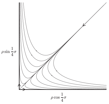
Figure 2: Conical geometry of the slow manifold. The twisted pairs are represented by the vertex. The two axes are identified under a nontrivial gauge transformation.

The loop of twisted pairs — the horizontal axis in Figure 1 — collapses to the vertex of the cone. The vertex of the cone looks like an index 1 fixed point lying on the boundary of ${\mathcal{A}/\mathcal{G}}$.

The outgoing trajectories at $\sigma=0$ and $\sigma=2\pi$, i.e., at $g_{\mathit{tw}}=+1$ and $g_{\mathit{tw}}=-1$, are gauge equivalent. The orientations of the small instanton and the small anti-instanton are lined up within $SU(2)$. Under the Y-M flow, the instanton and anti-instanton grow larger, presumably merging together and annihilating, flowing eventually to the flat connection. It remains to be proved that this does in fact happen in general, that the outgoing trajectory from the untwisted pair, $g_{\mathit{tw}}=\pm 1$, ends at the flat connection, and not at some other fixed point with $S_{\mathit{YM}}>0$. Here, we prove this only for the special case where the instanton and anti-instanton of the untwisted pair are located at opposite poles in $S^{4}$. Then the entire outgoing trajectory is $SO(4)$-invariant, and we can show that there are no $SO(4)$-invariant fixed points besides the flat connection and the untwisted pair itself.

2.4.1 Global stability

We have only established the local stability of the loop of twisted pairs. We can argue for global stability based on a theorem of Taubes [16] which states that, for connections in the trivial $SU(2)$ bundle over $S^{4}$, the hessian of $S_{\mathit{YM}}$ must have at least 2 negative eigenvalues at any smooth solution of the Yang-Mills equation (fixed point of the Y-M flow). It follows that there are no smooth fixed points with unstable manifolds of dimension 0 or 1. Any index 1 fixed point must be completely singular, so it must be a twisted pair or must have $S_{\mathit{YM}}\geq 4$. Therefore any loop of gauge fields with $S_{\mathit{YM}}<4$ must flow to the stable loop of twisted pairs. This argument does not work for stable 2-spheres, since Taubes’ theorem allows smooth fixed points of Morse index 2.

In retrospect, Taubes’ theorem and/or the paper of Uhlenbeck, Sibner, and Sibner could have made our numerical explorations unnecessary, leading directly to consideration of the loop of twisted pairs.

3 Preliminaries

We will be doing elementary, explicit calculations with the $U(2)$-invariant connections over $S^{4}$. In this section, we establish notation and collect some basic formulas. More detail is given in Appendix A.

3.1 Parametrization of $S^{3}$

We realize $S^{3}$ as the unit sphere in $\mathbb{C}^{2}$, parametrized by the unit vectors

$$\mathbf{z}=\begin{pmatrix}z_{1}\\ z_{2}\end{pmatrix}\,,\qquad\mathbf{z}^{\dagger}\mathbf{z}=\bar{z}_{1}z_{1}+\bar{z}_{2}z_{2}=1\,.$$ (12)

We write the complementary projection matrices

$$P(\mathbf{z})=\mathbf{z}\mathbf{z}^{\dagger}\,,\qquad Q(\mathbf{z})=1-P(\mathbf{z})\,.$$ (13)

The volume form on $S^{3}$ is

$$\mathrm{dvol}_{S^{3}}=-\frac{1}{2}(\mathbf{z}^{\dagger}d\mathbf{z})(d\mathbf{z}^{\dagger}d\mathbf{z})\,,\qquad\int_{S^{3}}\mathrm{dvol}_{S^{3}}=2\pi^{2}\,.$$ (14)

3.2 Parametrization of $S^{4}$

We realize $S^{4}$ as the unit sphere in $\mathbb{R}\oplus\mathbb{C}^{2}$, parametrized by the unit vectors

$$\vec{y}=(y_{0},\mathbf{y})\qquad y_{0}^{2}+\mathbf{y}^{\dagger}\mathbf{y}=1\,.$$ (15)

In polar coordinates,

$$\vec{y}=(\cos\theta,\mathbf{z}\sin\theta)\,,\qquad\mathbf{z}\in S^{3}\,.$$ (16)

Most often, we use coordinates $(x,\mathbf{z})$ where

$$x=\ln\tan\left(\frac{\theta}{2}\right)\,,\qquad-\infty\leq x\leq\infty\,.$$ (17)

The north pole of $S^{4}$ is at $\theta=0$, $x=-\infty$. The south pole is at $\theta=\pi$, $x=\infty$.

3.3 Round metric on $S^{4}$

The round metric on $S^{4}$ is

$$(ds)_{S^{4}}^{2}=R^{2}(x)\left[(dx)^{2}+d\mathbf{z}^{\dagger}d\mathbf{z}\right]\,,\qquad R^{2}(x)=(\cosh x)^{-2}\,.$$ (18)

3.4 Action of $U(2)$ on $S^{3}$ and $S^{4}$

$U\in U(2)$ acts on $S^{3}\subset\mathbb{C}^{2}$ by $\mathbf{z}\mapsto U\mathbf{z}$ and acts on $S^{4}\subset\mathbb{R}\oplus\mathbb{C}^{2}$ by $(y_{0},\mathbf{y})\mapsto(y_{0},U\mathbf{y})$ or $(x,\mathbf{z})\mapsto(x,U\mathbf{z})$.

3.5 $S^{3}$ identified with $SU(2)$

$S^{3}$ is identified with $SU(2)$ by

$$g(\mathbf{z})\mathbf{e}=\mathbf{z}\,,\qquad\mathbf{e}=\begin{pmatrix}1\\ 0\end{pmatrix}\,,\qquad g(\mathbf{z})=\begin{pmatrix}z_{1}&-\bar{z}_{2}\\ z_{2}&\bar{z}_{1}\end{pmatrix}\,.$$ (19)

The action of $U(2)$ on $S^{3}$ becomes

$$g(U\mathbf{z})=Ug(\mathbf{z})\begin{pmatrix}1&0\\ 0&(\det U)^{-1}\end{pmatrix}\,.$$ (20)

The rotation group $SO(4)$ is identified with $SU(2)\times SU(2)/\mathbb{Z}_{2}$ via

$$g(O(\mathbf{z}))=g_{L}g(\mathbf{z})g_{R}^{-1}\,,\qquad O\in SO(4)\,,\qquad(g_{L},g_{R})\in SU(2)\times SU(2)\,.$$ (21)

3.6 $U(2)$-invariant $su(2)$-valued 1-forms on $S^{3}$

The general $U(2)$-invariant $su(2)$-valued 1-form on $S^{3}$ is

$$f\eta-\bar{f}\eta^{\dagger}+f_{3}\eta_{3}\,,\qquad f_{3}\in\mathbb{R}\,,f\in\mathbb{C}$$ (22)

where

$$\eta =-PdP =-(\mathbf{z}^{\dagger}d\mathbf{z})\mathbf{z}\mathbf{z}^{\dagger}-\mathbf{z}d\mathbf{z}^{\dagger}$$ (23)

$$\eta^{\dagger} =-dPP =(\mathbf{z}^{\dagger}d\mathbf{z})\mathbf{z}\mathbf{z}^{\dagger}-d\mathbf{z}\mathbf{z}^{\dagger}$$ (24)

$$\eta_{3} =(\mathbf{z}^{\dagger}d\mathbf{z})(P-Q) =(\mathbf{z}^{\dagger}d\mathbf{z})(2\mathbf{z}\mathbf{z}^{\dagger}-1)$$ (25)

is a natural basis that diagonalizes the $U(1)$ generated by $i(P-Q)$,

$$[P-Q,\,\eta]=2\eta\,,\qquad[P-Q,\,\eta^{\dagger}]=-2\eta^{\dagger}\,,\qquad[P-Q,\,\eta_{3}]=0\,.$$ (26)

3.7 The Maurer-Cartan form $\omega$ on $SU(2)$

The Maurer-Cartan form $\omega$ on $SU(2)$ is

$$\omega=gd(g^{-1})=-\eta+\eta^{\dagger}-\eta_{3}\,,$$ (27)

satisfying

$$d\omega+\omega^{2}=0\,,\qquad-\frac{1}{6}\omega^{3}=\mathrm{dvol}_{S^{3}}\,1\,.$$ (28)

3.8 $U(2)$-invariant connections on $S^{4}$

A connection in the trivial $SU(2)$ bundle over $S^{4}$ is described by its covariant derivative

$$D=d+A(x,\mathbf{z})$$ (29)

where $A(x,\mathbf{z})$ is an $su(2)$-valued 1-form on $S^{4}$. Regularity at the poles requires

$$A(\pm\infty,\mathbf{z})=0\,.$$ (30)

Invariance under $U(2)$ is the condition

$$A(x,U\mathbf{z})=UA(x,\mathbf{z})U^{-1}\qquad U\in U(2)\,.$$ (31)

Define

$$d_{\omega}=gdg^{-1}=d+\omega$$ (32)

which satisfies

$$d_{\omega}^{2}=0\,,\qquad[d_{\omega},\,P-Q]=0\,.$$ (33)

The $U(1)$ generated by $i(P-Q)$ thus leaves $d_{\omega}$ invariant. It is convenient to write the $U(2)$-invariant connections in the $U(1)$-covariant form

$$D=d+A=d_{\omega}+\Delta A$$ (34)

$$\Delta A=A_{0}(x)dx\,i(P-Q)+f(x)\eta-\bar{f}(x)\eta^{\dagger}+f_{3}(x)\eta_{3}\$$ (35)

with

$$A_{0}(x)\,,f_{3}(x)\in\mathbb{R}\,,\;f(x)\in\mathbb{C}\,.$$ (36)

The $U(2)$-invariant gauge transformations act by

$$D\mapsto e^{i\varphi(x)(P-Q)}De^{-i\varphi(x)(P-Q)}=d_{\omega}-(\partial_{x}\varphi dx)\,i(P-Q)+e^{i\varphi(x)(P-Q)}\Delta Ae^{-i\varphi(x)(P-Q)}$$ (37)

$$e^{i\varphi(x)(P-Q)}\,\Delta A\,e^{-i\varphi(x)(P-Q)}=A_{0}(x)dx\,i(P-Q)+e^{2i\varphi(x)}f(x)\eta-e^{-2i\varphi(x)}\bar{f}(x)\eta^{\dagger}+f_{3}(x)\eta_{3}\,.$$ (38)

Connections with $A_{0}(x)=0$ are said to be in $A_{0}=0$ gauge. Any connection can be brought to $A_{0}=0$ gauge by the gauge transformation with $\partial_{x}\varphi=A_{0}(x)$, perhaps at the cost of introducing singularities at the poles $x=\pm\infty$.

3.9 The Yang-Mills action

The curvature 2-form is

$$F=D^{2}=dA+A^{2}\,.$$ (39)

The Yang-Mills action is

$$S_{YM}=\frac{1}{2\pi^{2}}\int_{S^{4}}\frac{1}{4}\mathrm{tr}(-F{*}F)$$ (40)

where $*$ is the Hodge operator taking $k$-forms to $(4-k)$-forms and satisfying ${*}^{2}=(-1)^{k}$.

For $U(2)$-invariant connections, the integrand is an invariant volume form

$$\frac{1}{4}\mathrm{tr}(-F{*}F)=dx\;L_{\mathit{YM}}(x)\,\mathrm{dvol}_{S^{3}}$$ (41)

and the Y-M action is

$$S_{YM}=\int_{-\infty}^{\infty}dx\,L_{\mathit{YM}}(x)\,.$$ (42)

3.10 Hodge duality

The (anti-)self-dual curvature is

$$F_{\pm}=\frac{1}{2}\left(F\pm{*}F\right)$$ (43)

The Y-M action splits into contributions of the two chiralities,

$$S_{\mathit{YM}}=S_{+}+S_{-}\qquad S_{\pm}=\frac{1}{2\pi^{2}}\int\frac{1}{4}\mathrm{tr}(-F_{\pm}{*}F_{\pm})\,.$$ (44)

The integer instanton number is

$$S_{\mathit{top}}=S_{+}-S_{-}\,.$$ (45)

The instanton number vanishes for connections in the trivial bundle over $S^{4}$.

3.11 Hodge duality for $U(2)$-invariant connections

For $U(2)$-invariant connections,

$$L_{\mathit{YM}}(x)=L_{+}(x)+L_{-}(x)$$ (46)

$$\frac{1}{4}\mathrm{tr}(-F_{\pm}{*}F_{\pm})=dx\,L_{\pm}(x)\;\mathrm{dvol}_{S^{3}}$$ (47)

$$S_{\pm}=\int_{-\infty}^{\infty}dx\,L_{\pm}(x)$$ (48)

$$S_{\mathit{YM}}=\int_{-\infty}^{\infty}dx\,\left[L_{+}(x)+L_{-}(x)\right]\,,\qquad S_{\mathit{top}}=\int_{-\infty}^{\infty}dx\,\left[L_{+}(x)-L_{-}(x)\right]\,.$$ (49)

For a $U(2)$-invariant connection in $A_{0}=0$ gauge,

$$D=d_{\omega}+\Delta A\,,\qquad\Delta A=f(x)\eta-\bar{f}(x)\eta^{\dagger}+f_{3}(x)\eta_{3}\,,$$ (50)

$$L_{\pm}=\frac{1}{4}\left[\partial_{x}f_{3}\pm 2\left(f_{3}-|f|^{2}\right)\right]^{2}+\frac{1}{2}\left|\partial_{x}f\pm 2\left(1-f_{3}\right)f)\right|^{2}$$ (51)

$$L_{\mathit{YM}}=\frac{1}{2}(\partial_{x}f_{3})^{2}+\left|\partial_{x}f\right|^{2}+2\left(f_{3}-|f|^{2}\right)^{2}+4\left(1-f_{3}\right)^{2}\left|f\right|^{2}$$ (52)

$$L_{+}-L_{-}=\partial_{x}\left(f_{3}^{2}+2\left|f\right|^{2}-2f_{3}\left|f\right|^{2}\right)\,,\qquad S_{\mathit{top}}=\left.\left(f_{3}^{2}+2\left|f\right|^{2}-2f_{3}\left|f\right|^{2}\right)\right|_{x=-\infty}^{x=\infty}\,.$$ (53)

3.12 Connections $d_{\omega}-f(x)\omega$

The $U(2)$-invariant connections that are invariant under the full $O(4)=SU(2)\times SU(2)/\{\pm 1\}$ are of the form

$$D=d_{\omega}-f(x)\omega=d_{\omega}+f(x)(\eta-\eta^{\dagger}+\eta_{3})\,.$$ (54)

Substituting in equations 51 and 53,

$$L_{\pm}(x)=\frac{3}{4}\left[\partial_{x}f\pm 2f(1-f)\right]^{2}\,.$$ (55)

$$S_{\mathit{top}}=\left.\left(3f^{2}-2f^{3}\right)\right|_{x=-\infty}^{x=\infty}\,.$$ (56)

3.13 The basic instanton

The BPST instanton [8] is the self-dual connection, $F=F_{+}$, of instanton number $1$. For us, the basic instanton is the self-dual $U(2)$-invariant connection of the form

$$D_{+}=d_{\omega}-f_{+}(x)\omega\,.$$ (57)

The self-duality equation $F_{-}=0$ becomes the ordinary differential equation

$$\partial_{x}f_{+}=2f_{+}(1-f_{+})\,.$$ (58)

The general solution is

$$f_{+}(x)=\frac{1}{1+e^{-2(x-x_{+})}}=\frac{1}{1+\rho_{+}^{-2}e^{-2x}}\,.$$ (59)

The parameter $\rho_{+}=e^{-x_{+}}$ is the size of the instanton. The Y-M action density is

$$L_{\mathit{YM}}(x)=L_{+}(x)=\frac{3}{4\cosh^{4}(x-x_{+})}$$ (60)

and the Y-M action is

$$S_{\mathit{YM}}=S_{+}=S_{\mathit{top}}=1\,.$$ (61)

The basic instanton is regular at the south pole ($x=\infty$), because $D_{+}\rightarrow d$ there. Near the north pole, $D_{+}\rightarrow d_{\omega}=gdg^{-1}$, so the instanton lives in the nontrivial bundle formed from trivial bundles over the two hemispheres, patched together at the equator using the index $+1$ map $\mathbf{z}\mapsto g(\mathbf{z})$ from $S^{3}$ to $SU(2)$. When the instanton size goes to zero, when $x_{+}\rightarrow\infty$, the action density becomes a delta-function concentrated at the south pole, at $x=\infty$. We say that the basic instanton is located at the south pole.

3.14 The basic anti-instanton

The anti-instanton is the anti-self-dual connection of instanton number $-1$. Our basic anti-instanton is

$$D_{-}=d_{\omega}-f_{-}(x)\omega$$ (62)

$$\partial_{x}f_{-}=-2f_{-}(1-f_{-})$$ (63)

$$f_{-}(x)=\frac{1}{1+e^{2(x-x_{-})}}=\frac{1}{1+\rho_{-}^{-2}e^{2x}}\,.$$ (64)

The parameter $\rho_{-}=e^{x_{-}}$ is the size of the anti-instanton. The basic instanton and anti-instanton are related by the orientation reversing map $x\mapsto-x$, $\rho_{+}\leftrightarrow\rho_{-}$. The Y-M action is

$$L_{\mathit{YM}}(x)=L_{-}(x)=\frac{3}{4\cosh^{4}(x-x_{-})}\,,\qquad S_{\mathit{YM}}=S_{-}=-S_{\mathit{top}}=1\,.$$ (65)

The basic anti-instanton is regular at the south pole ($x=-\infty$), because $D_{+}\rightarrow d$. Near the north pole, $D_{+}\rightarrow gdg^{-1}$, so the anti-instanton lives in the nontrivial bundle formed from trivial bundles on the hemispheres patched together at the equator using the index $-1$ map $\mathbf{z}\mapsto g(\mathbf{z})^{-1}$. When the anti-instanton size goes to zero, when $x_{-}\rightarrow-\infty$, the action density becomes a delta-function concentrated at the north pole, at $x=-\infty$. The basic anti-instanton is located at the north pole.

3.15 Twisted (anti-)instantons

The $U(2)$-invariant twisted instanton with twist angle $\sigma_{+}\in[0,2\pi]$ is

$$e^{i\alpha_{+}(x)(P-Q)}D_{+}e^{-i\alpha_{+}(x)(P-Q)}$$ (66)

where $\alpha(x)$ satisfies

$$\alpha_{+}(-\infty)=\frac{1}{2}\sigma_{+}\,,\qquad\alpha_{+}(\infty)=0\,.$$ (67)

and the $U(2)$-invariant twisted (anti-)instanton with twist angle $\sigma_{-}$ is

$$e^{i\alpha_{-}(x)(P-Q)}D_{-}e^{-i\alpha_{-}(x)(P-Q)}$$ (68)

$$\alpha_{-}(-\infty)=0\,,\quad\alpha_{-}(\infty)=\frac{1}{2}\sigma_{-}\,.$$ (69)

These are of course merely gauge transforms of the basic (anti-)instanton. The twist angle $\sigma_{\pm}$ is gauge invariant only if we restrict our notion of gauge equivalence to the group of pointed gauge transformations, that act as the identity at a base-point in $S^{4}$, here the gauge transformations $e^{i\varphi(x)(P-Q)}$ with $\varphi(\pm\infty)=0$.

The (anti-)instanton twisted by a general element $g_{\mathit{tw}}\in SU(2)/\{\pm 1\}$ is

$$D_{\pm}(g_{\mathit{tw}})=\phi(g_{\mathit{tw}})D_{\pm}\phi(g_{\mathit{tw}})^{-1}$$ (70)

where

$$\phi(g_{\mathit{tw}})(x,\mathbf{z})\rightarrow g(\mathbf{z})g_{\mathit{tw}}g(\mathbf{z})^{-1}\,,\qquad x\rightarrow\pm\infty\,.$$ (71)

The $U(2)$-invariant twisted (anti-)instanton corresponds to

$$g_{\mathit{tw}}=\begin{pmatrix}e^{\frac{1}{2}i\sigma_{\pm}}&0\\ 0&e^{-\frac{1}{2}i\sigma_{\pm}}\end{pmatrix}\,,\qquad g(\mathbf{z})g_{\mathit{tw}}g(\mathbf{z})^{-1}=e^{i\frac{1}{2}\sigma_{\pm}(P-Q)}$$ (72)

Rotations $O=(g_{L},g_{R})$ in $SO(4)=SU(2)\times SU(2)/\mathbb{Z}_{2}$ transform the twisted (anti-)instanton by

$$D_{\pm}(g_{\mathit{tw}})(x,O\mathbf{z})=g_{L}D_{\pm}(g_{R}^{-1}g_{\mathit{tw}}g_{R})(x,\mathbf{z})g_{L}^{-1}\,.$$ (73)

The $g_{R}$ act by conjugation on the twist $g_{\mathit{tw}}$, so every twisted instanton can be taken to a $U(2)$-invariant one by a rotation in $SO(4)$. The $g_{L}$ are symmetries, as are the $g_{R}$ that commute with $g_{tw}$.

3.16 Nontrivial $U(2)$-invariant maps $\phi_{h}:S^{4}\rightarrow SU(2)$

The Hopf fibration [2] is the map $h:S^{3}\rightarrow S^{2}\subset\mathbb{R}\oplus\mathbb{C}$,

$$h(\mathbf{z})=(|z_{1}|^{2}-|z_{2}|^{2},2\bar{z}_{1}z_{2})\,.$$ (74)

The nontrivial element in $\pi_{4}SU(2)=\mathbb{Z}_{2}$ is represented by the suspension, $Sh:S^{4}\rightarrow S^{3}=SU(2)$, of the Hopf fibration [3]. In particular, the $U(2)$-invariant maps $\phi_{h}:S^{4}\mapsto SU(2)$ of the form

$$\phi_{h}(x,\mathbf{z})=e^{i\varphi_{h}(x)(P-Q)}=g(\mathbf{z})\begin{pmatrix}e^{i\varphi_{h}(x)}&0\\ 0&e^{-i\varphi_{h}(x)}\end{pmatrix}g(\mathbf{z})^{-1}$$ (75)

with

$$\varphi_{h}(-\infty)=\pi\,,\qquad\varphi_{h}(\infty)=0$$ (76)

represent the nontrivial element in $\pi_{4}SU(2)=\mathbb{Z}_{2}$ [17]. Explictly,

$$\phi_{h}(x,\mathbf{z})=\cos\varphi_{h}(x)\begin{pmatrix}1&0\\ 0&1\end{pmatrix}+i\sin\varphi_{h}(x)\begin{pmatrix}|z_{1}|^{2}-|z_{2}|^{2}&2z_{1}\bar{z}_{2}\\ 2\bar{z}_{1}z_{2}&-|z_{1}|^{2}+|z_{2}|^{2}\end{pmatrix}\,.$$ (77)

4 Computer calculation

We start with a numerical calculation, looking for a clue to the long term behavior of the Y-M flow on the nontrivial loops. We pick a particular nontrivial loop and try to discover what it flows to. The calculation is sketched here. Details are given in Appendix B.

4.1 Rationale

We use the homogeneous space $SU(3)/SU(2)=S^{5}$ to construct a nontrivial loop of connections on $S^{4}$. The $SU(2)$ bundles over $S^{5}$ are classified topologically by $\pi_{4}SU(2)$, since they are made by gluing two trivial bundles along the equator in $S^{5}$ by a map from the equator, $S^{4}$, to $SU(2)$. The bundle $SU(2)\rightarrow SU(3)\rightarrow S^{5}$ represents the nontrivial element in $\pi_{4}SU(2)$ [4].

There is a canonical invariant connection $D_{\mathit{inv}}$ in $SU(2)\rightarrow SU(3)\rightarrow S^{5}$. We pull back $D_{\mathit{inv}}$ along a certain map $[-1,1]\times S^{4}\rightarrow S^{5}$ to obtain a one parameter family $D(s)$ of connections over $S^{4}$. The map is chosen so that the endpoint connections $D(\pm 1)$ are both flat, so $s\mapsto D(s)$ forms a closed loop in $\mathcal{A}/\mathcal{G}$. The nontriviality of the loop is verified explicitly in Appendix B. The map $[-1,1]\times S^{4}\rightarrow S^{5}$ preserves a $U(2)$ subgroup of the symmetries of $D_{\mathit{inv}}$, so each $D(s)$ is a $U(2)$-invariant connection over $S^{4}$.

We want to see what happens to this particular nontrivial loop under the Y-M flow. The Y-M flow preserves symmetry, so loop will remain within the $U(2)$-invariant connections on $S^{4}$. Two additional discrete symmetries of $D_{\mathit{inv}}$ are likewise preserved by our construction, one taking each $D(s)$ to itself, the other taking $D(s)$ to $D(-s)$. The connection $D(0)$ at the midpoint of the loop thus has an extra discrete symmetry. Again, the Y-M flow preserves these discrete symmetries.

In order to simplify the computational problem, we assume a plausible-seeming scenario. We assume that the midpoint $D(0)$ of the initial loop will flow to a fixed point in $\mathcal{A}/\mathcal{G}$ of Morse index 1, while the rest of the loop will flow to the one dimensional unstable manifold of the fixed point. The discrete symmetry that takes $D(s)$ to $D(-s)$ will exchange the two outgoing branches of the unstable manifold. Now we do not need to run the Y-M flow on the entire loop, but only on the single connection $D(0)$. We simplify still further by assuming that $D(0)$ will flow to a connection that minimizes $S_{\mathit{YM}}$ among all the $U(2)$-invariant conections with the same two discrete symmetries as $D(0)$. Assuming this scenario, there is no need to run the Y-M flow at all. We need only minimize $S_{\mathit{YM}}$ on this class of invariant connections, which is quite easy to do numerically. There is a fairly extensive literature on minimizing $S_{YM}$ over connections with specific prescribed symmetries [18, 14, 19, 20, 21, 22, 23, 24, 25, 26, 27, 13], but seemingly not the $U(2)\times\mathbb{Z}_{2}^{2}$ symmetry of interest here. The closest seems to be [25], which studies $U(2)$ invariant connections on non-round $S^{4}$ and finds a solution of the Yang-Mills equation which degenerates, in the round limit, to a zero-size instanton/anti-instanton pair.

The purpose of the numerical calculation is only heuristic. The simplifying assumptions are justified by the clue that emerges from the computation. It could have turned out otherwise. In particular, it could have turned out that an initial loop with such special symmetries would not detect generic properties of the Y-M flow acting on loops.

4.2 Numerical results

The midpoint connection $D(0)=d_{\omega}+\Delta A(0)$ of the initial loop is calculated in Appendix B,

$$\Delta A(0)=\cos\theta\,(\eta-\eta^{\dagger})+\left(1-\frac{1}{2}\sin^{2}\theta\right)\eta_{3}\,.$$ (78)

It is convenient to use the polar angle $\theta$ here, rather than $x=\ln\tan\frac{1}{2}\theta$ which we use elsewhere. The two discrete symmetries of $\Delta A(0)$ are derived in Appendix B. The general $U(2)$-invariant connection with these two additional discrete symmetries has the form

$$\Delta A=f(\theta)(\eta-\eta^{\dagger})+f_{3}(\theta)\eta_{3}$$ (79)

with

$$f=\bar{f}\qquad f(\pi-\theta)=-f(\theta)\qquad f_{3}(\pi-\theta)=f_{3}(\theta)\,.$$ (80)

Regularity at the poles requires the boundary conditions

$$f=f_{3}=1\;\text{ at }\theta=0\,.$$ (81)

We change variables again, to

$$t=\cos\theta$$ (82)

The Y-M action is given by equation 52,

$$S_{\mathit{YM}}=\int_{-1}^{1}dt\,(1-t^{2})^{-1}L_{\mathit{YM}}\,$$ (83)

$$L_{\mathit{YM}}=\frac{1}{2}(1-t^{2})^{2}(\partial_{t}f_{3})^{2}+2(f_{3}-f^{2})^{2}+(1-t^{2})^{2}(\partial_{t}f)^{2}+4(1-f_{3})^{2}f^{2}\qquad\,.$$ (84)

The initial connection $D(0)$ has

$$L_{YM}=\frac{3}{2}(1-t^{2})(1-t^{4})\,,\qquad S_{\mathit{YM}}=2.4\,.$$ (85)

To minimize $S_{\mathit{YM}}$ numerically, we use a finite mode approximation [23]. We write $f_{3}$ and $f$ as polynomials in $t$ obeying the symmetry and boundary conditions,

$$f_{3}=1+\sum_{n=1}^{N/2}(t^{2n}-1)a_{2n}\qquad f=t+\sum_{n=1}^{N/2}(t^{2n+1}-t)a_{2n-1}$$ (86)

where $N$ is an even number. The $N$ real variables $a_{k}$ parametrize an affine subspace of $\mathcal{A}$ of dimension $N$. We are approximating $\mathcal{A}$ by an increasing family of finite dimensional affine subspaces. On each subspace, $S_{\mathit{YM}}$ evaluates to a quartic polynomial in the $a_{k}$, which is minimized numerically using mathematical software such as Sage[28]. Typical results are shown in Table 1.

$N$	$\min(S_{\mathit{YM}})$
2	2.15627	12	2.00723	22	2.00286
4	2.06011	14	2.00504	24	2.00251
6	2.03019	16	2.00368	26	2.00202
8	2.01735	18	2.00346	28	2.00186
10	2.01086	20	2.00313	30	2.00147

Table 1: Results of numerical minimization of $S_{\mathit{YM}}$ on affine subspaces of $\mathcal{A}$ of dimension $N$.

The numerical results suggest that there is a global minimum with $S_{\mathit{YM}}=2$. The possibility of an integer global minimum motivates examining the self-dual and anti-self-dual action densities $L_{\pm}(x)$ of the approximate minima obtained from the computer calculations. Figure 3 plots the evolution of $L_{\pm}(x)$ as $N$ increases.

Figure 3: Plots of $L_{\pm}(x)$ for the connections numerically minimizing $S_{\mathit{YM}}$ for $N\leq 30$. The curves move away from the origin as $N$ increases. For comparison, the rightmost curve is $L_{+}(x)$ for the instanton of size $\rho_{+}=e^{-x_{+}}$, $x_{+}=4$.

It looks like the global minimum is a connection that consists of a zero-size instanton at the south pole and a zero-size anti-instanton at the north pole, and is otherwise flat. Closer inspection suggests that the minimum is attained at the connection given by

$$f_{3} =f=f_{-}=\frac{1}{1+e^{2(x-x_{-})}}\,, x<0$$ (87)

$$f_{3} =-f=f_{+}=\frac{1}{1+e^{-2(x-x_{+})}}\,, x>0$$ (88)

in the limit $x_{+}\rightarrow\infty$, $x_{-}\rightarrow-\infty$. This is the zero-size basic anti-instanton at the north pole combined with a twisted zero-size instanton at the south pole, twisted by $\pi$.

5 Twisted pairs

Motivated by the numerical calculation, we investigate the long time behavior of the Y-M flow near the singular connections that consist of a zero-size instanton and a zero-size anti-instanton patched together on a 3-sphere separating their locations. We are calling such connections twisted pairs. The general twisted pair is parametrized by the locations of the instanton and anti-instanton and by their relative twist $g_{\mathit{tw}}$. The $U(2)$-invariant twisted pair has the instanton at the south pole and the anti-instanton at the north pole and has diagonal $g_{\mathit{tw}}$, so is parametrized by the twist angle $\sigma\in[0,2\pi]$. We write the $U(2)$-invariant twisted pair explicitly in the next section. The general twisted pair is obtained by making a conformal transformation of $S^{4}$.

5.1 The $U(2)$-invariant twisted pairs

A $U(2)$-invariant twisted pair combines a $U(2)$-invariant twisted instanton of small size $\rho_{+}$ at the south pole with a $U(2)$-invariant twisted anti-instanton of the same size $\rho_{-}$ at the north pole, in the limit $\rho_{\pm}\rightarrow 0$,

$$D_{\mathit{tw}}(\alpha_{+},\alpha_{-})=\lim_{\rho_{\pm}\rightarrow 0}\left\{\begin{matrix}e^{i\alpha_{+}(x)(P-Q)}D_{-}e^{-i\alpha_{+}(x)(P-Q)}\quad&x>0\hfill\\[4.30554pt] e^{i\alpha_{-}(x)(P-Q)}D_{+}e^{-i\alpha_{-}(x)(P-Q)}\quad&x<0\,.\end{matrix}\right.$$ (89)

The functions $\alpha_{\pm}(x)$ should vanish fast enough at the poles to ensure that the connection is regular there,

$$\alpha_{\pm}(x)=O(e^{\mp 2x})\,,\qquad x\rightarrow\pm\infty\,.$$ (90)

The connection $D_{\mathit{tw}}(\alpha_{+},\alpha_{-})$ and its curvature are discontinuous at the equator as long as $\rho_{\pm}>0$, but the discontinuities disappear in the zero-size limit.

The relative twist is

$$\sigma=2\alpha_{+}(0)-2\alpha_{-}(0)\,.$$ (91)

The $U(2)$-invariant gauge transformations $e^{i\varphi(x)(P-Q)}$ act by $\alpha_{\pm}(x)\mapsto\alpha_{\pm}(x)-\varphi(x)$, so the relative twist $\sigma$ is gauge invariant. Any two $U(2)$-invariant twisted pairs with the same twist $\sigma$ are gauge equivalent.

5.2 The nontrivial loop of twisted pairs

The $U(2)$-invariant twisted pairs with twist $\sigma\in[0,2\pi]$ form a nontrivial closed loop in $\mathcal{A}/\mathcal{G}$ (for references on the nontriviality of such loops, reference [14] refers to reference [15]). To see this explicitly, let $D_{\mathit{tw}}(2\pi)=D_{\mathit{tw}}(\alpha_{+},\alpha_{-})$ be any twisted pair with $\sigma=2\alpha_{+}(0)-2\alpha_{-}(0)=2\pi$, and let $D_{\mathit{tw}}(0)=D_{\mathit{tw}}(0,0)$, which has twist $0$. Then

$$D_{\mathit{tw}}(2\pi)=\phi_{h}D_{\mathit{tw}}(0)\phi_{h}^{-1}$$ (92)

where $\phi_{h}$ is one of the nontrivial maps $S^{4}\rightarrow SU(2)$ described in section 3.16 above,

$$\phi_{h}(x,\mathbf{z})=e^{i\varphi_{h}(x)(P-Q)}\,,\qquad\varphi_{h}(x)=\left\{\begin{matrix}\alpha_{+}(x)\hfill\quad&x>0\hfill\\[4.30554pt] \pi+\alpha_{-}(x)\quad&x<0\,.\end{matrix}\right.$$ (93)

6 The slow manifold

A twisted pair is everywhere self-dual or anti-self-dual or flat, so the twisted pairs are all fixed points under the Y-M flow. Instantons in isolation are stable under the Y-M flow, as are anti-instantons. All perturbations of the instanton transverse to the space of instantons are driven rapidly to zero under the Y-M flow. Therefore, the Y-M flow, acting on a small neighborhood of the twisted pairs, rapidly compresses the neighborhood down to a space of approximate fixed points, the slow manifold, which is parametrized by an asymptotically small instanton and an asymptotically small anti-instanton. The long time behavior of the Y-M flow near the twisted pairs is determined by the flow on the slow manifold, which can be represented as a flow on the parameter space of the instanton-anti-instanton pair. To find the long time behavior, it will be enough to calculate the asymptotic expansion of the flow equation on the slow manifold to leading order in the sizes of the instanton and anti-instanton, at least if the leading order flow is robust against small perturbations.

The slow manifold is parametrized by the location, size and twist of the instanton and by the location, size and twist of the anti-instanton. A gauge transformation eliminates one of the twists, leaving the relative twist. The slow manifold is thus parametrized by the two locations, the two sizes and the relative twist $g_{\mathit{tw}}$.

The Y-M action $S_{\mathit{YM}}$ is invariant under the 15 parameter conformal group $SO(1,5)$, so $S_{\mathit{YM}}$ on the slow manifold, as a function of the parameters of the instanton-anti-instanton pair, is invariant under $SO(1,5)$. Therefore it suffices to calculate the generator of the Y-M flow, which is the gradient of $S_{\mathit{YM}}$, on a representative slice through the orbits of the conformal group.

We move the instanton to the south pole in $S^{4}$ using a conformal transformation, and the anti-instanton to the north pole using another. The remaining subgroup of $SO(1,5)$ consists of the rotation group $SO(4)$ and the translations in $x$ (which are the dilations of $\mathbb{R}^{4}$ in the stereographic projection). A rotation in $SO(4)$ diagonalizes the relative twist $g_{\mathit{tw}}$. We now have a $U(2)$-invariant instanton and a $U(2)$-invariant anti-instanton. A translation $x\mapsto x+a$ takes $\rho_{+}$ to $e^{-a}\rho_{+}$ and $\rho_{-}$ to $e^{a}\rho_{-}$, so we can use a translation in $x$ to set $\rho_{+}=\rho_{-}=\rho$. We now have a representative slice of the slow manifold parametrized by the $U(2)$-invariant instanton-anti-instanton pairs of equal size $\rho$ and relative twist $\sigma$.

7 The Y-M flow equation on the slow manifold

To calculate the asymptotic expansion of the Y-M flow equation on the slow manifold, we start with a larger than necessary slice of the slow manifold: all the $U(2)$-invariant instanton-anti-instanton pairs, parametrized by their asymptotically small sizes $\rho_{\pm}$ and their twist angles $\sigma_{\pm}\in[0,2\pi]$. This slice of the slow manifold is a family of $U(2)$-invariant connections

$$D^{\mathit{slow}}=\left\{\begin{matrix}e^{i\alpha_{+}(x)(P-Q)}\,(D_{+}+\delta A_{+})\,e^{-i\alpha_{+}(x)(P-Q)}\quad&x>0\hfill\\[4.30554pt] e^{i\alpha_{-}(x)(P-Q)}\,(D_{-}+\delta A_{-})\,e^{-i\alpha_{-}(x)(P-Q)}\hfill&x<0\,,\end{matrix}\right.$$ (94)

$$\alpha_{\pm}(0)=\frac{1}{2}\sigma_{\pm}\,.$$ (95)

The $\delta A_{\pm}$ are asymptotically small perturbations of the instanton and anti-instanton, to be determined by the condition that the family of connections $D^{\mathit{slow}}$, parametrized by $\rho_{\pm}$ and $\sigma_{\pm}$, is preserved under the Y-M flow. There must be velocity vector fields

$$\frac{d}{dt}\rho_{\pm}=\dot{\rho}_{\pm}\,,\qquad\frac{d}{dt}\alpha_{\pm}(x)=\dot{\alpha}_{\pm}(x)\,,\qquad\frac{d}{dt}\sigma_{\pm}=\dot{\sigma}_{\pm}=2\dot{\alpha}_{\pm}(0)$$ (96)

such that the Y-M flow equation is satisfied on the slow manifold

$$\frac{d}{dt}D^{\mathit{slow}}={*}D^{\mathit{slow}}{*}F^{\mathit{slow}}$$ (97)

where $F^{\mathit{slow}}$ is the curvature of $D^{\mathit{slow}}$. We solve for the velocities in two steps:

1. First we solve equation 97, the Y-M flow equation, separately in each open hemisphere. The general solution in each hemisphere depends on several undetermined parameters, including $\dot{\rho}_{\pm}$ and $\dot{\sigma}_{\pm}$.

2. Then we require $D^{\mathit{slow}}$ and $F^{\mathit{slow}}$ to be continuous at the equator, $x=0$, so that the flow equation holds there as well. At this stage, to simplify the calculation, we specialize to the subfamily where there is an $x\rightarrow-x$ symmetry, where

   $$\rho_{+}=\rho_{-}=\rho\,,\qquad\alpha_{+}(x)=-\alpha_{-}(-x)=\alpha(x)\,,\qquad\sigma_{+}=-\sigma_{-}=\frac{1}{2}\sigma\,.$$ (98)

   The symmetric twisted pairs still represent every orbit of the conformal group.

   The continuity conditions at $x=0$ fix all parameters in the separate solutions on the two hemispheres, thereby determining the velocity vectors $\dot{\rho}$, $\dot{\alpha}(x)$, and $\dot{\sigma}$.

All calculations are to leading order in $\rho$. With more work, the method would produce the velocity vectors on the slow manifold to all orders in $\rho$.

7.1 The flow equation in each open hemisphere

In this section, we solve the flow equation, equation 97, in each hemisphere separately, to leading order in $\rho_{\pm}$. The calculation is the same in each hemisphere, so, for the sake of legibility, we temporarily write $\rho$ instead of $\rho_{\pm}$ and $f$ instead of $f_{\pm}$.

The lhs of equation 97 is, to leading order,

$$\frac{d}{dt}D^{\mathit{slow}}=e^{i\alpha_{\pm}(x)(P-Q)}\,\left(\dot{\rho}\frac{\partial\hfill}{\partial\rho}D_{\pm}+\left[D_{\pm},\,-i\dot{\alpha}_{\pm}(x)(P-Q)\right]\right)\,e^{-i\alpha_{\pm}(x)(P-Q)}$$ (99)

We only need the rhs of equation 97 expanded to first order in $\delta A$. To this order, the connection $D=D_{\pm}+\delta A$ has curvature $F=D_{\pm}^{2}+D_{\pm}\delta A$ where $D_{\pm}^{2}$ is the curvature of the (anti-)instanton. So

$${*}D{*}F={*}[\delta A,\,D_{\pm}^{2}]+{*}D_{\pm}{*}D_{\pm}\delta A=\mp{*}D_{\pm}^{2}\delta A+{*}D_{\pm}{*}D_{\pm}\delta A={*}D_{\pm}({*}\mp 1)D_{\pm}\delta A$$ (100)

so the rhs of equation 97 becomes

$${*}D^{\mathit{slow}}{*}F^{\mathit{slow}}=e^{i\alpha_{\pm}(x)(P-Q)}\left[{*}D_{\pm}({*}\mp 1)D_{\pm}\delta A\right]e^{-i\alpha_{\pm}(x)(P-Q)}\,.$$ (101)

The flow equation, equation 97, is now

$$\dot{\rho}\frac{\partial\hfill}{\partial\rho}D_{\pm}+\left[D_{\pm},\,-i\dot{\alpha}_{\pm}(x)(P-Q)\right]={*}D_{\pm}({*}\mp 1)D_{\pm}\delta A\,.$$ (102)

This takes a particularly simple form if we make a change of basis

$$\omega=-\eta+\eta^{\dagger}-\eta_{3}\,,\qquad\omega_{1}=\eta-\eta^{\dagger}-2\eta_{3}\,,\qquad\omega_{2}=-i(\eta+\eta^{\dagger})\,.$$ (103)

Recall that

$$f=\frac{1}{1+\rho^{-2}e^{\mp 2x}}\,,\qquad\frac{1}{f}-1=\rho^{-2}e^{\mp 2x}$$ (104)

so

$$\rho\frac{\partial\hfill}{\partial\rho}D_{\pm}=\rho\frac{\partial\hfill}{\partial\rho}(d_{\omega}-f\omega)=-2f(1-f)\omega\,.$$ (105)

The $U(2)$-invariant infinitesimal gauge transformations of the (anti-)instanton are

$$\left[D_{\pm},\,-i\varphi(x)(P-Q)\right] =-\partial_{x}\varphi(x)dx\,i(P-Q)-\varphi(x)\left[-f\omega,\,i(P-Q)\right]$$ (106)

$$=-\partial_{x}\varphi(x)dx\,i(P-Q)-2f\varphi(x)\omega_{2}\,.$$ (107)

Using this formula with $\varphi=\dot{\alpha}_{\pm}$, equation 102 becomes

$$-2\rho^{-1}\dot{\rho}f(1-f)\omega-\partial_{x}\dot{\alpha}_{\pm}dx\,i(P-Q)-2f\dot{\alpha}_{\pm}\omega_{2}={*}D_{\pm}({*}\mp 1)D_{\pm}\delta A\,.$$ (108)

We expand in the new basis

$$\delta A=\delta A_{0}(x)dx\,i(P-Q)+\delta f(x)\omega+\delta A_{1}(x)\omega_{1}+\delta A_{2}(x)\omega_{2}\,.$$ (109)

The laplacian, derived in Appendix A.13, is diagonal in this basis,

$${*}D_{\pm}({*}\mp 1)D_{\pm}\delta A =-8R^{2}(x)^{-1}f^{2}\delta\tilde{A}_{0}idx(P-Q)-2R^{2}(x)^{-1}f^{-1}\partial_{x}\left(f^{2}\delta\tilde{A}_{0}\right)\omega_{2}$$ (110)

$$\qquad{}+R^{2}(x)^{-1}f^{-1}(1-f)^{-1}\partial_{x}f^{2}(1-f)^{2}\partial_{x}f^{-1}(1-f)^{-1}\delta f\,\omega$$ (111)

$$\qquad{}+R^{2}(x)^{-1}f^{-1}(1-f)^{2}\partial_{x}f^{2}(1-f)^{-4}\partial_{x}f^{-1}(1-f)^{2}\delta A_{1}\,\omega_{1}$$ (112)

where $R^{2}(x)=(\cosh x)^{-2}$ is the conformal factor in the round metric on $S^{4}$ as written in equation 18 and where

$$\delta\tilde{A}_{0}=\delta A_{0}-\frac{1}{2}\partial_{x}(f^{-1}\delta A_{2})\,.$$ (113)

Note that $\delta\tilde{A}_{0}$ vanishes for perturbations of the form $\delta A_{0}=-\partial_{x}\varphi$, $\delta A_{2}=-2f\varphi$, which are the infinitesimal gauge transformations of the (anti-)instanton as given in equation 107. So the laplacian annihilates the infinitesimal gauge transformations, as it should.

We take advantage of the infinitesimal gauge transformations to set $\delta A_{0}=0$, keeping the perturbation $\delta A$ in $A_{0}=0$ gauge. Then

$$\delta\tilde{A}_{0}=-\frac{1}{2}\partial_{x}(f^{-1}\delta A_{2})\,.$$ (114)

The flow equation, equation 108, is now four ordinary equations

$$-\partial_{x}\dot{\alpha}_{\pm} =-8R^{2}(x)^{-1}f^{2}\delta\tilde{A}_{0}$$ (115)

$$-2f\dot{\alpha}_{\pm} =-2R^{2}(x)^{-1}f^{-1}\partial_{x}\left(f^{2}\delta\tilde{A}_{0}\right)$$ (116)

$$-2\rho^{-1}\dot{\rho}f(1-f) =R^{2}(x)^{-1}f^{-1}(1-f)^{-1}\partial_{x}f^{2}(1-f)^{2}\partial_{x}f^{-1}(1-f)^{-1}\delta f$$ (117)

$$0 =R^{2}(x)^{-1}f^{-1}(1-f)^{2}\partial_{x}f^{2}(1-f)^{-4}\partial_{x}f^{-1}(1-f)^{2}\delta A_{1}\,.$$ (118)

Since we are solving the flow equation only to leading order, we expand

$$R^{2}(x)=(\cosh x)^{-2}=\frac{4f(1-f)}{\left[\rho^{-1}f+\rho(1-f)\right]^{2}}=4\rho^{2}f^{-1}(1-f)+O(\rho^{4})$$ (119)

and keep only the leading order term. This approximation expresses the fact that, in the limit $\rho\rightarrow 0$, only the metric at the location of the (anti-)instanton enters into the solution of the flow equation. The four equations 115–118 become

$$\partial_{x}\dot{\alpha}_{\pm} =2\rho^{-2}f^{3}(1-f)^{-1}\delta\tilde{A}_{0}$$ (120)

$$\dot{\alpha}_{\pm} =\frac{1}{4}\rho^{-2}f^{-1}(1-f)^{-1}\partial_{x}\left(f^{2}\delta\tilde{A}_{0}\right)$$ (121)

$$\rho^{-1}\dot{\rho} =-\frac{1}{8}\rho^{-2}f^{-1}(1-f)^{-3}\partial_{x}f^{2}(1-f)^{2}\partial_{x}f^{-1}(1-f)^{-1}\delta f$$ (122)

$$0 =\partial_{x}f^{2}(1-f)^{-4}\partial_{x}f^{-1}(1-f)^{2}\delta A_{1}\,.$$ (123)

For $D^{\mathit{slow}}$ to be regular at the pole, the perturbations must vanish at $x=\pm\infty$,

$$\delta f=\delta A_{1}=\delta A_{2}=O(e^{\mp 2x})=O(1-f)\quad\qquad x\rightarrow\pm\infty\,,\;f\rightarrow 1\,.$$ (124)

7.1.1 The first two flow equations

The first of the four flow equations, equation 120, is trivially solved to give

$$\delta\tilde{A}_{0}=\frac{1}{2}\rho^{2}f^{-3}(1-f)\partial_{x}\dot{\alpha}_{\pm}\,.$$ (125)

Then the second of the four flow equations, equation 121, becomes an equation on $\dot{\alpha}_{\pm}(x)$,

$$8f(1-f)\dot{\alpha}_{\pm}=\partial_{x}\left[f^{-1}(1-f)\partial_{x}\dot{\alpha}_{\pm}\right]\,.$$ (126)

If we change independent variable from $x$ to $f(x)$,

$$df=\pm 2f(1-f)dx\,,$$ (127)

this becomes

$$2\dot{\alpha}_{\pm}=\partial_{f}(1-f)^{2}\partial_{f}\dot{\alpha}_{\pm}$$ (128)

which has two independent solutions, $1-f$ and $(1-f)^{-2}$. The latter is singular at the pole $x=\pm\infty$, so we must have

$$\dot{\alpha}_{\pm}=C_{\alpha{\pm}}(1-f)\,.$$ (129)

At $x=0$, this is

$$\dot{\alpha}_{\pm}(0)=\frac{C_{\alpha{\pm}}}{1+\rho^{2}}$$ (130)

so, to leading order,

$$C_{\alpha{\pm}}=\frac{1}{2}\dot{\sigma}_{\pm}\,,\qquad\dot{\alpha}_{\pm}=\frac{1}{2}\dot{\sigma}_{\pm}(1-f)\,.$$ (131)

Using equations 131 and 114 in equation 125, we get

$$\partial_{x}(f^{-1}\delta A_{2})=-\frac{1}{4}\rho^{2}\dot{\sigma}_{\pm}\partial_{x}\left[f^{-2}(1-f)^{2}\right]\,.$$ (132)

The unique solution that goes to zero at the pole, where $f=1$, is

$$\delta A_{2}=-\frac{1}{4}\rho^{2}\dot{\sigma}_{\pm}f^{-1}(1-f)^{2}\,.$$ (133)

We now have the general solution of the first two equations,

$$\delta A_{2}=-\frac{1}{4}\rho^{2}\dot{\sigma}_{\pm}f^{-1}(1-f)^{2}\,,\qquad\dot{\alpha}_{\pm}=\frac{1}{2}\dot{\sigma}_{\pm}(1-f)\,.$$ (134)

7.1.2 The last two flow equations

The last two of the four flow equations, equations 122 and 123, become, after the change of independent variable from $x$ to $f(x)$,

$$-2\rho\dot{\rho}(1-f)^{2} =\partial_{f}f^{3}(1-f)^{3}\partial_{f}f^{-1}(1-f)^{-1}\delta f$$ (135)

$$0 =\partial_{f}f^{3}(1-f)^{-3}\partial_{f}f^{-1}(1-f)^{2}\delta A_{1}\,.$$ (136)

Integrating once, we get

$$\frac{2}{3}\rho\dot{\rho}f^{-3} =\partial_{f}f^{-1}(1-f)^{-1}\delta f$$ (137)

$$-2C_{1}\rho^{2}f^{-3}(1-f)^{3} =\partial_{f}f^{-1}(1-f)^{2}\delta A_{1}\,.$$ (138)

The integration constant in the first equation is fixed by the boundary condition that $\delta f$ should go to zero at $f=1$. We write the integration constant in the second equation as $-2C_{1}\rho^{2}$ for later convenience.

Integrating again, we get

$$\delta f =-\frac{1}{3}\rho\dot{\rho}f^{-1}(1-f)+C_{f}f(1-f)$$ (139)

$$\delta A_{1} =C_{1}\rho^{2}\left[f^{-1}+2-6(1-f)^{-1}-6f(1-f)^{-2}\ln f\right]\,.$$ (140)

The integration constant $C_{f}$ can be absorbed into a redefinition of $\rho$, so we set $C_{f}=0$. The new integration constant in the second equation is fixed by the boundary condition at $f=1$.

7.1.3 Summary: the general solution in each hemisphere

Now we restore the $\pm$ subscripts to $\rho$ and $f$, indicating the hemisphere in which they obtain. The general solution to the flow equation in each hemisphere, with the gauge fixing condition $\delta A_{0\pm}=0$, is

$$\delta f_{\pm} =-\frac{1}{3}\rho_{\pm}\dot{\rho}_{\pm}f_{\pm}^{-1}(1-f_{\pm})$$ (141)

$$\delta A_{1{\pm}} =C_{1{\pm}}\rho_{\pm}^{2}\left[f_{\pm}^{-1}+2-6(1-f_{\pm})^{-1}-6f_{\pm}(1-f_{\pm})^{-2}\ln f_{\pm}\right]$$ (142)

$$\delta A_{2\pm} =-\frac{1}{4}\rho_{\pm}^{2}\dot{\sigma}_{\pm}f_{\pm}^{-1}(1-f_{\pm})^{2}$$ (143)

$$\dot{\alpha}_{\pm}(x) =\frac{1}{2}\dot{\sigma}_{\pm}(1-f_{\pm})\,.$$ (144)

The solution in each hemisphere is parametrized by three quantities, $\dot{r}_{\pm}$, $\dot{\sigma}_{\pm}$ and $C_{1\pm}$, which are to be determined by the continuity equations at the equator.

7.2 Continuity conditions at the equator

Now we specialize to the subfamily of connections $D^{\mathit{slow}}$ with

$$\rho_{+}=\rho_{-}=\rho\,,\qquad\sigma_{+}=-\sigma_{-}=\frac{1}{2}\sigma\,,\qquad\alpha_{+}(x)=-\alpha_{-}(-x)=\alpha(x)\,.$$ (145)

These connections $D^{\mathit{slow}}$ have an $x\mapsto-x$ symmetry that simplifies the calculations. The general solution to the flow equation in each hemisphere is now

$$\delta A_{0\pm} =0$$ (146)

$$\delta f_{\pm} =-\frac{1}{3}\rho\dot{\rho}f_{\pm}^{-1}(1-f_{\pm})$$ (147)

$$\delta A_{1{\pm}} =C_{1{\pm}}\rho^{2}\left[f_{\pm}^{-1}+2-6(1-f_{\pm})^{-1}-6f_{\pm}(1-f_{\pm})^{-2}\ln f_{\pm}\right]$$ (148)

$$\delta A_{2\pm} =\mp\frac{1}{8}\rho^{2}\dot{\sigma}f_{\pm}^{-1}(1-f_{\pm})^{2}$$ (149)

$$\dot{\alpha}_{\pm} =\pm\frac{1}{4}\dot{\sigma}(1-f_{\pm})$$ (150)

$$\alpha_{\pm}(0) =\pm\frac{1}{4}\sigma$$ (151)

We will need, at $x=0$, the values

$$\delta f_{\pm}(0)=-\frac{1}{3}\rho^{-1}\dot{\rho}\,,\qquad\delta A_{1{\pm}}(0)=C_{1{\pm}}\,,\qquad\delta A_{2\pm}(0)=\mp\frac{1}{8}\dot{\sigma}\,,$$ (152)

and the first derivatives

$$\partial_{x}\delta f_{\pm}(0)=\pm\frac{2}{3}\rho^{-1}\dot{\rho}\,,\qquad\partial_{x}\delta A_{1{\pm}}(0)=\mp 2C_{1{\pm}}\,,\qquad\partial_{x}\delta A_{2\pm}(0)=\frac{1}{4}\dot{\sigma}\,.$$ (153)

7.2.1 Continuity of $D^{\mathit{slow}}$

The continuity of $D^{\mathit{slow}}$ at the equator is the condition, at $x=0$,

$$e^{i\alpha_{+}(x)(P-Q)}\,(D_{+}+\delta A_{+})\,e^{-i\alpha_{+}(x)(P-Q)}=e^{i\alpha_{-}(x)(P-Q)}\,(D_{-}+\delta A_{-})\,e^{-i\alpha_{-}(x)(P-Q)}\,.$$ (154)

This is equivalent to

$$e^{\frac{1}{4}i\sigma(P-Q)}\,(-\rho^{2}\omega+\delta A_{+})\,e^{-\frac{1}{4}i\sigma(P-Q)}=e^{-\frac{1}{4}i\sigma(P-Q)}\,(-\rho^{2}\omega+\delta A_{-})\,e^{\frac{1}{4}i\sigma(P-Q)}$$ (155)

since $D_{\pm}=d_{\omega}-f_{\pm}\omega$ and $\partial_{x}\alpha_{+}(0)=\partial_{x}\alpha_{-}(0)$ by the symmetry $\alpha_{-}(x)=-\alpha_{+}(-x)$ and

$$f_{+}(0)=f_{-}(0)=\rho^{2}+O(\rho^{4})\,.$$ (156)

At $x=0$,

$$-\rho^{2}\omega+\delta A_{\pm} =\left(-\rho^{2}-\frac{1}{3}\rho^{-1}\dot{\rho}\right)\omega+C_{1{\pm}}\omega_{1}\mp\frac{1}{8}\dot{\sigma}\omega_{2}$$ (157)

$$=\left(\rho^{2}+\frac{1}{3}\rho^{-1}\dot{\rho}+C_{1{\pm}}\pm\frac{1}{8}i\dot{\sigma}\right)\eta-\left(\rho^{2}+\frac{1}{3}\rho^{-1}\dot{\rho}+C_{1{\pm}}\mp\frac{1}{8}i\dot{\sigma}\right)\eta^{\dagger}$$ (158)

$$\qquad{}+\left(\rho^{2}+\frac{1}{3}\rho^{-1}\dot{\rho}-2C_{1{\pm}}\right)\eta_{3}$$ (159)

so the continuity condition becomes the two equations

$$e^{\frac{1}{2}i\sigma}\left(\rho^{2}+\frac{1}{3}\rho^{-1}\dot{\rho}+C_{1{+}}+\frac{1}{8}i\dot{\sigma}\right) =e^{-\frac{1}{2}i\sigma}\left(\rho^{2}+\frac{1}{3}\rho^{-1}\dot{\rho}+C_{1{-}}-\frac{1}{8}i\dot{\sigma}\right)$$ (160)

$$\rho^{2}+\frac{1}{3}\rho^{-1}\dot{\rho}-2C_{1{+}} =\rho^{2}+\frac{1}{3}\rho^{-1}\dot{\rho}-2C_{1{-}}$$ (161)

which are equivalent to the two equations

$$C_{1+}=C_{1-}$$ (162)

and

$$\left(\rho^{2}+\frac{1}{3}\rho^{-1}\dot{\rho}+C_{1{+}}\right)\sin\frac{1}{2}\sigma=-\frac{1}{8}\dot{\sigma}\cos\frac{1}{2}\sigma\,.$$ (163)

7.2.2 Continuity of $F^{\mathit{slow}}$

Continuity of $F^{\mathit{slow}}$ at $x=0$ is

$$e^{\frac{1}{4}i\sigma(P-Q)}\,(D_{+}^{2}+D_{+}\delta A_{+})\,e^{-\frac{1}{4}i\sigma(P-Q)}=e^{-\frac{1}{4}i\sigma(P-Q)}\,(D_{-}^{2}+D_{-}\delta A_{-})\,e^{\frac{1}{4}i\sigma(P-Q)}$$ (164)

The self-dual part of this condition is

$$e^{\frac{1}{4}i\sigma(P-Q)}\,(2D_{+}^{2}+({*}+1)D_{+}\delta A_{+})\,e^{-\frac{1}{4}i\sigma(P-Q)}=e^{-\frac{1}{4}i\sigma(P-Q)}\,({*}+1)D_{-}\delta A_{-}\,e^{\frac{1}{4}i\sigma(P-Q)}$$ (165)

while the anti-self-dual part is

$$e^{\frac{1}{4}i\sigma(P-Q)}\,({*}-1)D_{+}\delta A_{+}\,e^{-\frac{1}{4}i\sigma(P-Q)}=e^{-\frac{1}{4}i\sigma(P-Q)}\,(-2D_{-}^{2}+({*}-1)D_{-}\delta A_{-})\,e^{\frac{1}{4}i\sigma(P-Q)}\,.$$ (166)

The self-dual and anti-self-dual continuity equations are equivalent under the $x\mapsto-x$ symmetry.

From Appendix A.6, the (anti-)instanton curvature is

$$D_{\pm}^{2}=-2f_{\pm}(1-f_{\pm})({*}\pm 1)dx\omega$$ (167)

which is, at $x=0$,

$$D_{\pm}^{2}=-2\rho^{2}({*}\pm 1)dx\omega\,.$$ (168)

From Appendix A.13,

$$D_{\pm}\delta f_{\pm}\omega =\partial_{x}\delta f_{\pm}dx\omega+\lambda\delta f_{\pm}{*}dx\omega$$ (169)

$$D_{\pm}\delta A_{1\pm}\omega_{1} =\partial_{x}\delta A_{1\pm}dx\omega_{1}+\lambda_{1}\delta A_{1\pm}{*}dx\omega_{1}$$ (170)

$$D_{\pm}\delta A_{2\pm}\omega_{2} =\partial_{x}\delta A_{2\pm}dx\omega_{2}+\lambda_{2}\delta A_{2\pm}{*}dx\omega_{2}$$ (171)

where, to leading order,

$$\lambda=\lambda_{1}=\lambda_{2}=2\,.$$ (172)

At $x=0$, using the values collected in equations 152 and 153,

$$D_{\pm}\delta f_{\pm}\omega =-\frac{2}{3}\rho^{-1}\dot{\rho}({*}\mp 1)dx\omega$$ (173)

$$D_{\pm}\delta A_{1\pm}\omega_{1} =2C_{1\pm}({*}\mp 1)dx\omega_{1}$$ (174)

$$D_{\pm}\delta A_{2\pm}\omega_{2} =\mp\frac{1}{4}\dot{\sigma}({*}\mp 1)dx\omega_{2}$$ (175)

so

$$D_{\pm}\delta A_{\pm}=({*}\mp 1)dx\left(-\frac{2}{3}\rho^{-1}\dot{\rho}\omega+2C_{1\pm}\omega_{1}\mp\frac{1}{4}\dot{\sigma}\omega_{2}\right)\,.$$ (176)

Equation 165, the self-dual continuity condition, becomes

$$e^{\frac{1}{4}i\sigma(P-Q)}\,\rho^{2}\omega\,e^{-\frac{1}{4}i\sigma(P-Q)}=e^{-\frac{1}{4}i\sigma(P-Q)}\,\left(\frac{1}{3}\rho^{-1}\dot{\rho}\omega-C_{1\pm}\omega_{1}-\frac{1}{8}\dot{\sigma}\omega_{2}\right)\,e^{\frac{1}{4}i\sigma(P-Q)}\,.$$ (177)

Equation 166, the anti-self-dual continuity condition, becomes the equivalent equation

$$e^{\frac{1}{4}i\sigma(P-Q)}\left(\frac{1}{3}\rho^{-1}\dot{\rho}\omega-C_{1\pm}\omega_{1}+\frac{1}{8}\dot{\sigma}\omega_{2}\right)e^{-\frac{1}{4}i\sigma(P-Q)}=e^{-\frac{1}{4}i\sigma(P-Q)}\,\rho^{2}\omega\,e^{\frac{1}{4}i\sigma(P-Q)}\,.$$ (178)

Their solution is

$$C_{1+} =\frac{1}{3}\rho^{2}(\cos\sigma-1)$$ (179)

$$\rho^{-1}\dot{\rho} =\rho^{2}(1+2\cos\sigma)$$ (180)

$$\dot{\sigma} =-8\rho^{2}\sin\sigma\,.$$ (181)

where we have used $C_{1+}=C_{1-}$ which was required for continuity of $D^{\mathit{slow}}$. Finally, we check that the remaining continuity condition on $D^{\mathit{slow}}$, equation 163, is now also satisfied.

7.3 Summary: the Y-M flow equation on the slow manifold

The slow manifold is represented by the family of $U(2)$-invariant connections

$$D^{\mathit{slow}}=\left\{\begin{matrix}e^{i\alpha_{+}(x)(P-Q)}\,(D_{+}+\delta A_{+})\,e^{-i\alpha_{+}(x)(P-Q)}&\qquad x>0\\[4.30554pt] e^{i\alpha_{-}(x)(P-Q)}\,(D_{-}+\delta A_{-})\,e^{-i\alpha_{-}(x)(P-Q)}\hfill&\qquad x<0\,.\end{matrix}\right.$$ (182)

obeying the symmetry condition

$$\rho_{+}=\rho_{-}=\rho\qquad\alpha_{+}(x)=-\alpha_{-}(-x)=\alpha(x)\,.$$ (183)

The relative twist of the instanton and anti-instanton is

$$\sigma=4\alpha(0)\,.$$ (184)

The slow manifold is parametrized by the instanton size $\rho$, the relative twist $\sigma$, and by the gauge function $\alpha(x)$, $\alpha(0)=\frac{1}{4}\sigma$. The gauge transformations

$$D^{\mathit{slow}}\mapsto e^{i\varphi(x)(P-Q)}D^{\mathit{slow}}e^{-i\varphi(x)(P-Q)}\,,\qquad\varphi(x)=-\varphi(-x)$$ (185)

act on the slow manifold by

$$\alpha(x)\mapsto\alpha(x)+\varphi(x)$$ (186)

so the slow manifold in $\mathcal{A}/\mathcal{G}$ is parametrized by $\rho$ and $\sigma$ alone.

The Y-M flow equations on the slow manifold are

$$\dot{\rho} =\rho^{3}(1+2\cos\sigma)+O(\rho^{5})$$ (187)

$$\dot{\sigma} =-8\rho^{2}\sin\sigma+O(\rho^{4})$$ (188)

$$\dot{\alpha} =\frac{1}{4}\dot{\sigma}(1-f_{+})+O(\rho^{4})\,.$$ (189)

The perturbation $\delta A_{\pm}$ of the (anti-)instanton is

$$\delta A_{\pm}=\delta f_{\pm}(x)\omega+\delta A_{1\pm}(x)\omega_{1}+\delta A_{2\pm}(x)\omega_{2}$$ (190)

where

$$\delta f_{\pm} =-\frac{1}{3}\rho^{4}(1+2\cos\sigma)f_{\pm}^{-1}(1-f_{\pm})+O(\rho^{6})$$ (191)

$$\delta A_{1{\pm}} =\frac{1}{3}\rho^{4}(\cos\sigma-1)\left[f_{\pm}^{-1}+2-6(1-f_{\pm})^{-1}-6f_{\pm}(1-f_{\pm})^{-2}\ln f_{\pm}\right]+O(\rho^{6})$$ (192)

$$\delta A_{2\pm} =2\rho^{4}\sin\sigma f_{\pm}^{-1}(1-f_{\pm})^{2}+O(\rho^{6})\,.$$ (193)

which indeed is a small perturbation of the (anti-)instanton $D_{\pm}$ everywhere on $S^{4}$.

8 The gradient formula and $S_{\mathit{YM}}$ on the slow manifold

We check that the Y-M flow on the slow manifold is a gradient flow with respect to the metric induced from the space of connections $\mathcal{A}$.

Let $dD^{\mathit{slow}}$ be an infinitesimal variation in the slow manifold, corresponding to variations $d\rho$ and $d\alpha(x)$ of the parameters. In the metric on $\mathcal{A}$, given by equation 6, the length-squared of the variation is

$$(ds^{2})^{\mathit{slow}}=\frac{1}{4\pi^{2}}\int_{S^{4}}\mathrm{tr}\left(-dD^{\mathit{slow}}{*}dD^{\mathit{slow}}\right)$$ (194)

In each hemisphere, to leading order,

$$dD^{\mathit{slow}}=e^{i\alpha_{\pm}(x)(P-Q)}\,\left(d\rho_{\pm}\frac{\partial\hfill}{\partial\rho_{\pm}}D_{\pm}+\left[D_{\pm},\,-id\alpha_{\pm}(x)(P-Q)\right]\right)\,e^{-i\alpha_{\pm}(x)(P-Q)}$$ (195)

with

$$d\rho_{\pm}\frac{\partial\hfill}{\partial\rho_{\pm}}D_{\pm} =-2\rho_{\pm}^{-1}d\rho_{\pm}f_{\pm}(1-f_{\pm})\omega$$ (196)

$$\left[D_{\pm},\,-id\alpha_{\pm}(x)(P-Q)\right] =-\partial_{x}d\alpha_{\pm}dx\,i(P-Q)-2f_{\pm}d\alpha_{\pm}\omega_{2}\,.$$ (197)

Using the inner-product formulas given in Appendix A.11, equation 430, we get

$$(ds^{2})^{\mathit{slow}}=\int_{-\infty}^{\infty}dx\,R^{2}(x)\left[12\rho_{\pm}^{-2}(d\rho_{\pm})^{2}f_{\pm}^{2}(1-f_{\pm})^{2}+(\partial_{x}d\alpha_{\pm})^{2}+8f_{\pm}^{2}(d\alpha_{\pm})^{2}\right]$$ (198)

We replace the conformal factor $R^{2}(x)$ by its leading order approximation, equation 119, getting

$$(ds^{2})^{\mathit{slow}}=\int_{-\infty}^{\infty}dx\,4\rho_{\pm}^{2}f_{\pm}^{-1}(1-f_{\pm})\left[12\rho_{\pm}^{-2}(d\rho_{\pm})^{2}f_{\pm}^{2}(1-f_{\pm})^{2}+(\partial_{x}d\alpha_{\pm})^{2}+8f_{\pm}^{2}(d\alpha_{\pm})^{2}\right]$$ (199)

Specializing to the $x\leftrightarrow-x$ symmetric subfamily, and again writing $f$ for $f_{+}$, we have

$$(ds^{2})^{\mathit{slow}} =2\int_{0}^{\infty}dx\,4\rho^{2}f^{-1}(1-f)\left[12\rho^{-2}(d\rho)^{2}f^{2}(1-f)^{2}+(\partial_{x}d\alpha)^{2}+8f^{2}(d\alpha)^{2}\right]$$ (200)

$$=16\int_{0}^{1}df\,\left[3(d\rho)^{2}(1-f)^{2}+\rho^{2}(1-f)^{2}(\partial_{f}d\alpha)^{2}+2\rho^{2}(d\alpha)^{2}\right]$$ (201)

$$=16(d\rho)^{2}+16\rho^{2}\int_{0}^{1}df\,\left[(1-f)^{2}(\partial_{f}d\alpha)^{2}+2(d\alpha)^{2}\right]$$ (202)

The generator of the Y-M flow, $\dot{\rho}$, $\dot{\alpha}$, has inner product with a general variation

$$(ds^{2})^{\mathit{slow}}(\dot{\rho},\dot{\alpha};d\rho,d\alpha) =16\dot{\rho}d\rho+16\rho^{2}\int_{0}^{1}df\,\left[(1-f)^{2}\partial_{f}\dot{\alpha}\partial_{f}d\alpha+2\dot{\alpha}d\alpha\right]$$ (203)

$$=16\dot{\rho}d\rho+4\dot{\sigma}\rho^{2}\int_{0}^{1}df\,\partial_{f}\left[-(1-f)^{2}d\alpha\right]$$ (204)

$$=16\dot{\rho}d\rho+\dot{\sigma}\rho^{2}d\sigma$$ (205)

$$=16\rho^{3}(1+2\cos\sigma)d\rho-8\rho^{2}\sin\sigma\rho^{2}d\sigma$$ (206)

so

$$(ds^{2})^{\mathit{slow}}(\dot{\rho},\dot{\alpha};d\rho,d\alpha)=-dS_{\mathit{YM}}$$ (207)

with

$$S_{\mathit{YM}}=2-4\rho^{4}(1+2\cos\sigma)+O(\rho^{6})\,.$$ (208)

This is the gradient formula, equation 5. The additive constant in $S_{YM}$ is fixed because $S_{\mathit{YM}}=2$ for the twisted pairs at $\rho=0$.

9 The metric on the slow manifold in $\mathcal{A}/\mathcal{G}$

The metric on the slow manifold in $\mathcal{A}$ is given by equation 202. To find the metric on the slow manifold in $\mathcal{A}/\mathcal{G}$, we need to project on the horizontal subspace of the tangent space of $\mathcal{A}$ — the variations orthogonal to the infinitesimal gauge transformations.

The infinitesimal gauge transformations are the perturbations $d\alpha_{V}(x)$ with $d\alpha_{V}(0)=0$. A variation $d\alpha_{H}$ is perpendicular to the gauge transformations iff, for all $d\alpha_{V}(x)$ with $d\alpha_{V}(0)=0$,

$$\int_{0}^{1}df\,\left[(1-f)^{2}(\partial_{f}d\alpha_{V})(\partial_{f}d\alpha_{H})+2(d\alpha_{V})(d\alpha_{H})\right]=0$$ (209)

which is to say that $d\alpha_{H}$ satisfies the ordinary differential equation

$$\left[-\partial_{f}(1-f)^{2}\partial_{f}+2\right]d\alpha_{H}=0\,.$$ (210)

The only solution that vanishes at $f=1$ is

$$d\alpha_{H}=\frac{1}{4}d\sigma(1-f)\,.$$ (211)

Substituting in equation 202, we get the metric on the slow manifold in $\mathcal{A}/\mathcal{G}$,

$$(ds^{2})^{\mathit{slow}}_{\mathcal{A}/\mathcal{G}}=16(d\rho)^{2}+\rho^{2}(d\sigma)^{2}\,.$$ (212)

The gradient formula of course holds here as well,

$$(ds^{2})^{\mathit{slow}}_{\mathcal{A}/\mathcal{G}}(\dot{\rho},\dot{\sigma};d\rho,d\sigma)=-dS_{\mathit{YM}}\,.$$ (213)

10 Long time behavior of the flow

The Y-M flow on the slow manifold,

$$\frac{d\rho}{dt}=\rho^{3}(1+2\cos\sigma)\,,\qquad\frac{d\sigma}{dt}=-8\rho^{2}\sin\sigma\,,$$ (214)

has flow lines given by

$$\frac{d\rho}{d\sigma}=-\frac{\rho}{8}\left(\frac{1+2\cos\sigma}{\sin\sigma}\right)$$ (215)

which integrates to

$$\rho^{8}(1-\cos\sigma)\sin\sigma=4C\,.$$ (216)

Changing variable from $\sigma$ to

$$s=\cos\frac{\sigma}{2}\,,\qquad s\in[-1,1]\,,$$ (217)

the flow is

$$\frac{d\rho}{dt}=\rho^{3}(4s^{2}-1)\,,\qquad\frac{ds}{dt}=8\rho^{2}s(1-s^{2})\,,$$ (218)

and the flow lines are

$$\rho^{8}s(1-s^{2})^{3/2}=C\,.$$ (219)

On a flow line, say on the side $s\geq 0$ where $C\geq 0$, the flow equation is

$$\frac{ds}{dt}=8C^{1/4}(1-s^{2})^{5/8}s^{3/4}\,.$$ (220)

which integrates to

$$2C^{1/4}t=s_{t}^{\frac{1}{4}}F(s_{t}^{2})-s_{0}^{\frac{1}{4}}F(s_{0}^{2})$$ (221)

where $H(s^{2})$ is the hypergeometric function

$$F(z)=F\left({\textstyle\frac{1}{8}},{\textstyle\frac{5}{8}};{\textstyle\frac{9}{8}};z\right)\,,\qquad F(0)=1\,,\quad F(1-\epsilon)=F(1)-\frac{1}{3}\epsilon^{\frac{3}{8}}+O(\epsilon)\,.$$ (222)

Substituting for $C$, we get

$$2\rho_{0}^{2}(1-s_{0}^{2})^{3/8}t=\left(\frac{s_{t}}{s_{0}}\right)^{\frac{1}{4}}F(s_{t}^{2})-F(s_{0}^{2})$$ (223)

$$2\rho_{t}^{2}(1-s_{t}^{2})^{3/8}t=F(s_{t}^{2})-\left(\frac{s_{0}}{s_{t}}\right)^{\frac{1}{4}}F(s_{0}^{2})$$ (224)

Suppose $t$ large. If we hold $\rho_{0}$ fixed and letting $s_{0}$ vary near 0, we see explicitly from these formulas that the trajectory moves first towards $\rho=0$,$s=0$, then along the $s$-axis to the neighborhood of $\rho=0$, $s=1$, then outward to increasing $\rho$ with $s$ near 1.

11 The outgoing trajectory

For the symmetric twisted pair, where the instanton and anti-instanton are located at opposite poles in the round $S^{4}$, we can show that the outgoing trajectory at $\sigma=0,2\pi$ ends at the flat connection. The argument does not work for other twisted pairs, whose outgoing trajectories have less symmetry.

The perturbations $\delta A_{1,2}$, equations 192 and 193 vanish for $\sigma=0,2\pi$, so the outgoing trajectory has the full $SO(4)$ symmetry of the aligned instanton-anti-instanton and of the round geometry on $S^{4}$. The connections on the outgoing trajectory are therefore all of the form

$$D=d_{\omega}-f\omega\,,\qquad f(\pm\infty)=1\,.$$ (225)

From equation 55, the Y-M action is

$$S_{\mathit{YM}}=\int dx\,\frac{3}{2}\left[(\partial_{x}f)^{2}+4f^{2}(1-f)^{2}\right]\,.$$ (226)

From Appendix A,

$${*}F_{\pm} =-\left[\partial_{x}f\pm 2f(1-f)\right]\frac{1}{2}({*}\pm 1)dx\omega$$ (227)

$${*}D{*}F_{\pm} =-\frac{1}{2}R^{2}(x)^{-1}\left[\partial_{x}\pm 2(2f-1)\right]\left[\partial_{x}f\pm 2f(1-f)\right]\omega$$ (228)

so the Y-M flow equation is

$$\frac{df}{dt}=R^{2}(x)^{-1}\left[\partial_{x}^{2}f+4f(1-f)(2f-1)\right]\,.$$ (229)

Let us assume that the flow ends at a fixed point. The fixed point equation is

$$\partial_{x}^{2}f+4f(1-f)(2f-1)=0\,.$$ (230)

For any solution $f$ of the fixed point equation, the quantity

$$A=(\partial_{x}f)^{2}-4f^{2}(1-f)^{2}$$ (231)

is constant, $\partial_{x}A=0$, and must vanish because $S_{\mathit{YM}}<\infty$. So, for all $x$,

$$\partial_{x}f=\pm 2f(1-f)\,.$$ (232)

The only solution of this equation compatible with the boundary conditions $f(\pm\infty)=1$, besides the twisted pair, is $f=1$, the flat connection. There is no other fixed point where the outgoing trajectory can end.

12 Stable 2-manifolds of $SU(2)$ and $SU(3)$ gauge fields

Nontrivial stable 2-spheres of gauge fields might give 2-d instanton corrections to the space-time quantum field theory in the lambda model (discussed in section 13.3 below). Nontrivial 2-spheres of gauge fields are classified by $\pi_{2}(\mathcal{A}/\mathcal{G})$, which is $\pi_{5}$ of the gauge group. Potentially interesting examples are $\pi_{5}SU(2)=\mathbb{Z}_{2}$ and $\pi_{5}SU(3)=\mathbb{Z}$. We describe some partial results towards constructing stable 2-spheres for $SU(3)$ and for $SU(2)$ gauge groups.

12.1 $SU(3)$

Numerical evidence suggests that there is a stable 2-sphere of $SU(3)$ connections on $S^{4}$ consisting again of zero-size instanton-anti-instanton twisted pairs [29]. The numerical calculation is analogous to the $SU(2)$ calculation reported above (and was actually done first). The $SU(3)$ principle bundles over $S^{6}$ are classified by $\pi_{5}SU(3)=\mathbb{Z}$. The homogeneous space $SU(3)\rightarrow G_{2}\rightarrow S^{6}$ represents a generator of $\pi_{5}SU(3)$ [30]. Pulling back along a suitably chosen map $S^{2}\times S^{4}\rightarrow S^{6}$ gives a nontrivial 2-sphere of connections in the trivial $SU(3)$ bundle over $S^{4}$, representing a generator of $\pi_{2}(\mathcal{A}/\mathcal{G})$. The south pole of $S^{4}$ is mapped to the flat connection. Some of the $G_{2}$ symmetry survives, so that all of the connections on $S^{4}$ are $SU(2)$-invariant. An additional $U(1)$ symmetry acts on the 2-sphere family of connections, rotating the 2-sphere around its poles. The north pole of the 2-sphere is left fixed, so the connection at the north pole has an additional $U(1)$ symmetry. It also has a discrete symmetry exchanging $x\rightarrow-x$. It seems plausible that this connection flows to an index 2 fixed point whose two dimensional unstable manifold is a stable 2-sphere. It also seems plausible that this connection flows to the connection that minimizes $S_{\mathit{YM}}$ among all connections with the same symmetries. Carrying out this minimization of $S_{\mathit{YM}}$ numerically, we find strong indications that the minimum value is $S_{\mathit{YM}}=2$, realized by a twisted pair.

All $SU(3)$ instantons on $S^{4}$ of instanton number $\pm 1$ are reducible [31]. That is, they are $SU(2)$ instantons embedded in $SU(3)$. We identify $SU(2)$ with the upper-left $2\times 2$ block in $SU(3)$, identifying an element $g\in SU(2)$ with the block matrix

$$g\in SU(2)\equiv\left(\begin{array}[]{c|c}g&0\\ \hline\cr 0&1\end{array}\right)\in SU(3)\,.$$ (233)

The basic $SU(2)$ instanton $D_{+}$ is now an $SU(3)$ instanton. The general $SU(3)$ instanton — of given size and location — is $GD_{+}G^{-1}$ for $G\in SU(3)$, up to the equivalence $G\sim GK(\theta)$, for $K(\theta)$ in the $U(1)$ subgroup of $SU(3)$ of elements that commute with $SU(2)$, which take the block matrix form

$$K(\theta)=\left(\begin{array}[]{c|c}e^{i\theta}&0\\ \hline\cr 0&e^{-2i\theta}\end{array}\right)\,.$$ (234)

The space of orientations of the $SU(3)$ instanton is thus $SU(3)/U(1)$. The space of relative twists of a twisted pair of $SU(3)$ instantons is $M_{\mathit{tw}}^{SU(3)}=U(1)\backslash SU(3)/U(1)$, which consists of the individual orientations of the instanton and anti-instanton, $SU(3)/U(1)\times SU(3)/U(1)$, modulo the global $SU(3)$ gauge transformations. $M_{\mathit{tw}}^{SU(3)}$ contains nontrivial 2-spheres, $\pi_{2}M_{\mathit{tw}}^{SU(3)}\supset\mathbb{Z}$, that can represent $\pi_{2}(\mathcal{A}/\mathcal{G})$.

To write a concrete nontrivial 2-sphere of relative twists, it is convenient to parametrize $SU(3)$ as $SU(2)\times D^{2}\times SU(2)$,

$$G(g_{-},u,g_{+})=g_{-}^{-1}G_{1}(u)g_{+}$$ (235)

where

$$G_{1}(u)=\begin{pmatrix}1&0&0\\ 0&u&-\sqrt{1-|u|^{2}}\\ 0&\sqrt{1-|u|^{2}}&\bar{u}\end{pmatrix}\,,\qquad|u|\leq 1\,.$$ (236)

The parametrization is faithful for $|u|<1$, while at the boundary of the 2-disk, $|u|=1$, it gives a redundant parametrization of the subgroup $SU(2)\times U(1)\subset SU(3)$. The $U(1)$ subgroup of $SU(3)$ acts on the left and right by

$$K(\theta)G(g_{-},u,g_{+})K(\theta^{\prime})^{-1}=G(h({\theta+2\theta^{\prime}})g_{-},e^{2i\theta-2i\theta^{\prime}}u,h({2\theta+\theta^{\prime}})g_{+})$$ (237)

where

$$h(\theta)=\begin{pmatrix}e^{i\theta}&0\\ 0&e^{-i\theta}\end{pmatrix}\,.$$ (238)

The $O(4)=SU(2)\times SU(2)/\{\pm 1\}$ group of rotations around the poles of $S^{4}$ acts on the relative twists by $(g_{L},g_{R}):G\mapsto g_{R}^{-1}Gg_{R}$, the $g_{L}$ all leaving the twisted pair invariant. In our parametrization of $SU(3)$, the symmetries act by

$$G(g_{-},u,g_{+})\mapsto G(g_{-}g_{R},u,g_{+}g_{R})$$ (239)

We represent the symmetry classes of twists by the $G(1,u,g_{+})$ subject to the gauge equivalence

$$G(1,u,g_{+})\equiv G(1,e^{2i\theta}u,h(\theta)g_{+})=K\left(\frac{2\theta}{3}\right)G(1,u,g_{+})K\left(-\frac{\theta}{3}\right)^{-1}$$ (240)

and a remaining $U(1)$ symmetry

$$G(1,u,g_{+})\mapsto G(1,u,h({\theta})g_{+}h({\theta})^{-1})\,.$$ (241)

The symmetry classes of twisted pairs with an additional $U(1)$ invariance are the $G(1,u,1)$ and also $G(1,0,g_{0})$ with

$$g_{0}=\begin{pmatrix}0&1\\ -1&0\end{pmatrix}\,.$$ (242)

The latter, $G(1,0,g_{0})$, is the $U(2)$-invariant twisted pair indicated by the computer calculation.

A 2-sphere family of twisted pairs invariant under $U(1)$ acting by rotation around the poles of $S^{2}$ is given by

$$G(w)=G(1,w^{2},g_{1}(w))\,,\qquad|w|\leq 1$$ (243)

where

$$g_{1}(w)=\begin{pmatrix}w&-\sqrt{1-|w|^{2}}\\ \sqrt{1-|w|^{2}}&\bar{w}\end{pmatrix}\,.$$ (244)

The $U(1)$ symmetry is

$$G(w)\mapsto G(e^{i\theta}w)\,.$$ (245)

The twisted pair at the north pole of $S^{2}$, $w=0$, is the $U(2)$-invariant $G(1,0,g_{0})$. At $|w|=1$,

$$G(w)=K(w)\equiv 1$$ (246)

so $|w|=1$ can be identified to the the south pole in $S^{2}$, which is mapped to the aligned twisted pair, $G=1$.

It should be straightforward to check directly that $w\mapsto G(w)$ represents a generator of $\pi_{2}(\mathcal{A}/\mathcal{G})$, by the same argument used above to check the nontriviality of the loop of $SU(2)$ twisted pairs. We leave $A_{0}=0$ gauge, making $G(w)D_{+}G(w)^{-1}$ non-singular at the south pole of $S^{4}$ by a gauge transformation $\phi(w,x)\in SU(3)$. The twisted pairs at $|w|=1$ will all be gauge equivalent, giving a loop in the gauge group, a map $S^{1}\times S^{4}\rightarrow SU(3)$. This will factor through a map $S^{5}\rightarrow SU(3)$, which we can check is a generator of $\pi_{5}SU(3)$ by composing with $SU(3)\rightarrow S^{5}=SU(3)/SU(2)$ to get a map $S^{5}\rightarrow S^{5}$ whose index should be $\pm 1$ [4].

A quicker way to check the nontriviality of the 2-sphere $w\mapsto G(w)$ is to evaluate the family index [32] of the Dirac operator on $S^{4}$ acting on spinors tensored with the defining representation, $\mathbf{3}$, of $SU(3)$. The chiral zero-modes of the Dirac operator of each handedness are localized respectively in the instanton and and the anti-instanton. It is a simple calculation to show that the left-handed zero mode forms a line bundle of Chern number 1 over the 2-sphere of twisted pairs, which must then necessarily be a generator of $\pi_{2}(\mathcal{A}/\mathcal{G})=\mathbb{Z}$.

The Y-M flow on the slow manifold remains to be calculated in order to check that that the 2-sphere $w\mapsto G(w)$, or some deformation, is locally stable under the flow. The calculation is the same, in principle, as for the $SU(2)$ twisted pairs. For $SU(3)$, the symmetry classes of twists are described by 3 parameters, analogous to the twist angle $\sigma$ for $SU(2)$ twists. Unfortunately, there does seem to be any symmetry that singles out a distinguished set of representatives of the symmetry classes, closed under the flow, analogous to the $U(2)$ symmetry for $SU(2)$ twisted pairs. It might be possible to find a perpendicular slice through the symmetry classes, which would be closed under the gradient flow. Otherwise, it will be necessary to parametrize the slow manifold by the full 6 parameter space of $SU(3)$ twists, in addition to the instanton size $\rho$. Inverting the instanton laplacian will be considerably more work than in the $SU(2)$ case. In any case, the calculation of the Y-M flow on the slow manifold and the check of local stability remain to be done.

12.2 $SU(2)$

Since $\pi_{5}SU(2)=\mathbb{Z}_{2}$, there should be a nontrivial stable 2-sphere of $SU(2)$ gauge fields on $S^{4}$. We do not know of a homogeneous realization of the generator of $\pi_{5}SU(2)$ analogous to the bundles $SU(2)\rightarrow SU(3)\rightarrow S^{5}$ for $\pi_{4}SU(2)$ and $SU(3)\rightarrow G_{2}\rightarrow S^{6}$ for $\pi_{5}SU(3)$, but there is available a realization with enough symmetry to reduce the problem to minimizing $S_{\mathit{YM}}$ on the space of connections with a certain fixed symmetry group, as in the other two cases. In this case, the symmetry group is large enough that numerical minimization is (barely) practical.

We construct a nontrivial 2-sphere family of $SU(2)$ bundles over $S^{4}$, each having the symmetry group $(U(1)\times U(1)/\mathbb{Z}_{2})\times\mathbb{Z}_{2}$. The bundle at the north pole in $S^{2}$ has an extra $\mathbb{Z}_{2}\times\mathbb{Z}_{2}$ symmetry. We attempt to minimize $S_{\mathit{YM}}$ numerically over connections with the enhanced symmetry group $(U(1)\times U(1)/\mathbb{Z}_{2})\times(\mathbb{Z}_{2})^{3}$, again approximating the space of such connections by finite dimensional affine subspaces. We find $\min(S_{\mathit{YM}})<4.0053$. The numerical computations are more expensive in processing time and memory than the previous ones because the two continuous symmetries reduce $S^{4}$ to a 2-dimensional domain, instead of the 1-dimensional domain of the previous calculations. We have to minimize $S_{\mathit{YM}}$ over connections that are polynomials in two variables.

The numerical results suggest that, at the enhanced symmetry point in the 2-sphere family, $\min(S_{\mathit{YM}})$ is realized by a fixed point of the Y-M flow that consists of two zero-size instantons and two zero-size anti-instantons, arranged along the $x$ axis in the order $\bar{I}I\bar{I}I$. Writing the sizes of the instantons $r_{+1}=e^{-x_{+1}}$, $r_{+2}=e^{x_{+2}}$ and the sizes of the anti-instantons $r_{-1}=e^{x_{-1}}$, $r_{-2}=e^{-x_{-2}}$, the zero-size limit is taken with

$$x_{-1}\ll x_{+2}\ll 0\ll x_{-2}\ll x_{+1}\,.$$ (247)

Each pair of neighbors in the sequence is maximally twisted. It seems plausible that repulsion between neighbors will drive such a configuration of finite-size instantons and anti-instantons to this zero-size limit. In the limit, there is an an instanton/anti-instanton pair at each of the poles.

The evidence for $\min(S_{\mathit{YM}})=4$ at the enhanced symmetry point, realized by the twisted quadruplet of zero-size (anti-)instantons, is good, though perhaps not as compelling as in the previous calculations. The twisted quadruplet has $S_{\mathit{YM}}=4$, so $S_{\mathit{YM}}\leq 4$ is a rigorous upper bound at the enhanced symmetry point.

The continuous $U(1)\times U(1)/\mathbb{Z}_{2}$ symmetry restricts the relative twists of the instantons to the diagonal $SU(2)$ matrices. We write explicitly a 2-parameter family of twisted quadruplet connections, in the 2-parameter family of bundles. This family of connections forms a 2-torus, not a 2-sphere. It remains to calculate the Y-M flow in the slow modes, to check first that the twisted quadruplet connection at the enhanced symmetry point has a 2-dimensional unstable manifold, and then to find the global structure of that unstable manifold, presumably either a 2-torus of zero area or a 2-sphere of nonzero area. The first possibility would be of interest for the lambda model.

12.2.1 A nontrivial 2-sphere of $SU(2)$ bundles over $S^{4}$

The nontrivial element in $\pi_{5}SU(2)$ was originally realized as the suspension map $S(h\circ Sh):S^{5}\rightarrow S^{3}$, where $h:S^{3}\rightarrow S^{2}$ is the Hopf fibration, and $Sh:S^{4}\rightarrow S^{3}$ is its suspension [6]. We write explicitly

$$S(h\circ Sh):[0,\pi]^{2}\times SU(2)\rightarrow SU(2)$$ (248)

$$S(h\circ Sh)(\beta_{1},\beta_{2},g)=\left(gh_{\beta_{2}}g^{-1}\right)^{-1}h_{\beta_{1}}\left(gh_{\beta_{2}}g^{-1}\right)$$ (249)

where

$$h_{\beta}=\begin{pmatrix}e^{i\beta}&0\\ 0&e^{-i\beta}\end{pmatrix}\,.$$ (250)

We make a topologically insignificant modification, defining

$$\Phi_{2}:[0,\pi]^{2}\times SU(2)\rightarrow SU(2)$$ (251)

$$\Phi_{2}(\beta_{1},\beta_{2})(g)=h_{\beta_{1}}^{-1}S(h\circ Sh)=h_{\beta_{1}}^{-1}\left(gh_{\beta_{2}}g^{-1}\right)^{-1}h_{\beta_{1}}\left(gh_{\beta_{2}}g^{-1}\right)\,,$$ (252)

which satisfies

$$\Phi_{2}(\beta_{1},0,g)=\Phi_{2}(\beta_{1},\pi,g)=\Phi_{2}(0,\beta_{2},g)=\Phi_{2}(\pi,\beta_{2},g)=1\,,$$ (253)

so the boundary of the square $[0,\pi]^{2}$ can be identified to a point, the square becoming a 2-sphere, and $\Phi_{2}$ becoming a nontrivial map $S^{2}\times SU(2)\rightarrow SU(2)$. For each $(\beta_{1},\beta_{2})\in S^{2}$, we construct an $SU(2)$ bundle over $S^{4}$ using $g\mapsto\Phi_{2}(\beta_{1},\beta_{2},g)$ as the gluing map at the equator in $S^{4}$. Thus $\Phi_{2}$ defines a nontrivial 2-sphere of trivial $SU(2)$ bundles over $S^{4}$.

The group $SO(4)=SU(2)\times SU(2)/\{\pm 1\}$ of rotations of $S^{4}$ around the polar axis acts by

$$\Phi_{2}(\beta_{1},\beta_{2},g_{L}gg_{R}^{-1})=g_{L}\left[h_{1}^{-1}\left(gh_{2}g^{-1}\right)^{-1}h_{1}\left(gh_{2}g^{-1}\right)\right]g_{L}^{-1}$$ (254)

where

$$h_{1}=g_{L}^{-1}h_{\beta_{1}}g_{L}\,,\qquad h_{2}=g_{R}^{-1}h_{\beta_{2}}g_{R}\,.$$ (255)

If $g_{L}$ and $g_{R}$ are both diagonal,

$$g_{L}=h_{\alpha^{\prime}}\,,\qquad g_{R}=h_{\alpha}\,,$$ (256)

then

$$\Phi_{2}(\beta_{1},\beta_{2},h_{\alpha^{\prime}}gh_{\alpha}^{-1})=h_{\alpha^{\prime}}\Phi_{2}(\beta_{1},\beta_{2},g)h_{\alpha^{\prime}}^{-1}$$ (257)

so each of the $SU(2)$ bundles over $S^{4}$ is invariant under the $U(1)\times U(1)/\{\pm 1\}$ subgroup of diagonal matrices $(h_{\alpha^{\prime}},h_{\alpha})$ modulo $(-1,-1)$.

In addition, the entire 2-sphere family of bundles is invariant under the $\mathbb{Z}_{2}\times\mathbb{Z}_{2}$ subgroup generated by $(g_{L},g_{R})=(\mu_{2},\mu_{2})$ and $(\mu_{1},\mu_{3})$ where

$$\mu_{1}=\begin{pmatrix}0&i\\ i&0\end{pmatrix}\,,\qquad\mu_{2}=\begin{pmatrix}0&1\\ -1&0\end{pmatrix}\,,\qquad\mu_{3}=\begin{pmatrix}i&0\\ 0&-i\end{pmatrix}\,.$$ (258)

This $\mathbb{Z}_{2}\times\mathbb{Z}_{2}$ acts on the family of bundles by

$$\Phi_{2}(\beta_{1},\beta_{2},\mu_{2}g\mu_{2}^{-1}) =\mu_{2}\Phi_{2}(\pi-\beta_{1},\pi-\beta_{2},g)\mu_{2}^{-1}$$ (259)

$$\Phi_{2}(\beta_{1},\beta_{2},\mu_{1}g\mu_{3}^{-1}) =\mu_{1}\Phi_{2}(\pi-\beta_{1},\beta_{2},g)\mu_{1}^{-1}$$ (260)

$$\Phi_{2}(\beta_{1},\beta_{2},\mu_{3}g\mu_{1}) =\mu_{3}\Phi_{2}(\beta_{1},\pi-\beta_{2},g)\mu_{3}^{-1}\,.$$ (261)

Finally, there is a $\mathbb{Z}_{2}$ symmetry

$$\Phi_{2}(\beta_{1},\beta_{2},g)^{-1}=h_{\beta_{1}}^{-1}\Phi_{2}(\pi-\beta_{1},\beta_{2},g)h_{\beta_{1}}$$ (262)

that acts by reflecting $S^{4}$ in the equator, taking $\theta\rightarrow\pi-\theta$, $x\rightarrow-x$. Combining with the discrete symmetry $g\mapsto\mu_{1}g\mu_{3}^{-1}$, we get a reflection symmetry of each bundle in the family,

$$\Phi_{2}(\beta_{1},\beta_{2},g)^{-1}=h_{\beta_{1}}^{-1}\mu_{1}^{-1}\Phi_{2}(\beta_{1},\beta_{2},\mu_{1}g\mu_{3}^{-1})\mu_{1}h_{\beta_{1}}$$ (263)

so each connection has symmetry group $(U(1)\times U(1)/\{\pm 1\})\times\mathbb{Z}_{2}$.

The $SU(2)$ bundle at the midpoint $\beta_{1}=\beta_{2}=\frac{\pi}{2}$ thus has an extra $\mathbb{Z}_{2}\times\mathbb{Z}_{2}$ symmetry. If we were to choose a 2-sphere family of connections in this 2-sphere family of $SU(2)$ bundles, respecting the symmetries of the bundles, then run the Y-M flow on the family of connections, we might expect that the connection at the midpoint $\beta_{1}=\beta_{2}=\frac{\pi}{2}$ would flow to a fixed point with effective Morse index 2 that minimizes $S_{\mathit{YM}}$ among all connections with the enhanced symmetry of the bundle at $\beta_{1}=\beta_{2}=\frac{\pi}{2}$. With this scenario in mind, we attempt to minimize $S_{\mathit{YM}}$ among the connections invariant under this $(U(1)\times U(1)/\{\pm 1\})\times(\mathbb{Z}_{2})^{3}$ group.

12.2.2 Reduction to 2-dimensions

The continuous symmetry group $U(1)\times U(1)/\{\pm 1\}$ acts on $S^{4}$ by

$$g=\begin{pmatrix}z_{1}&-\bar{z}_{2}\\ z_{2}&\bar{z}_{1}\end{pmatrix}\mapsto h_{\alpha^{\prime}}gh_{\alpha}^{-1}=\begin{pmatrix}z_{1}e^{i\alpha^{\prime}-i\alpha}&-\bar{z}_{2}e^{i\alpha^{\prime}+i\alpha}\\ z_{2}e^{-i\alpha^{\prime}-i\alpha}&\bar{z}_{1}e^{-i\alpha^{\prime}+i\alpha}\end{pmatrix}=\begin{pmatrix}z_{1}e^{i\alpha_{1}}&-\bar{z}_{2}e^{-i\alpha_{2}}\\ z_{2}e^{i\alpha_{2}}&\bar{z}_{1}e^{-i\alpha_{1}}\end{pmatrix}$$ (264)

$$\alpha^{\prime}=\frac{1}{2}(\alpha_{1}-\alpha_{2})\,,\qquad\alpha=\frac{1}{2}(-\alpha_{1}-\alpha_{2})\,.$$ (265)

We write

$$z_{1}=r_{1}e^{i\theta_{1}}\,,\qquad z_{2}=r_{2}e^{i\theta_{2}}\,,\qquad r_{1}=\cos\frac{1}{2}\psi\,,\qquad r_{2}=\sin\frac{1}{2}\psi\,,\qquad\psi\in[0,\pi]$$ (266)

and use $\theta,\psi,\theta_{1},\theta_{2}$ as coordinates on $S^{4}$. We can write the coordinate map

$$g=h_{\frac{1}{2}(\theta_{1}-\theta_{2})}g(\psi)h_{\frac{1}{2}(-\theta_{1}-\theta_{2})}^{-1}$$ (267)

where

$$g(\psi)=\begin{pmatrix}r_{1}&-r_{2}\\ r_{2}&r_{1}\end{pmatrix}=e^{-\frac{1}{2}\psi\mu_{2}}\,.$$ (268)

The coordinate map is redundant at the poles $\theta=0,\pi$ and at $\psi=0,\pi$. All of $S^{4}$ is covered when $\psi$ ranges over $[0,\pi]$, but it is useful to think of $\psi$ taking any real value, the coordinate map being many-to-one.

The slice $\theta_{1}=\theta_{2}=0$ contains one representative in each symmetry class (except at the poles $\theta=0,\pi$). A connection on $S^{4}$ invariant under the continuous symmetry will reduce to a connection on the slice, the 2-dimensional domain parametrized by $\theta$ and $\psi$.

A connection in the bundle defined by the patching map $\Phi_{2}(\beta_{1},\beta_{2})$ consists of a connection in each hemisphere, $D_{\pm}=d+A_{\pm}$, related on the overlap of the hemispheres by

$$D_{-}=\Phi_{2}(\beta_{1},\beta_{2})D_{+}\Phi_{2}(\beta_{1},\beta_{2})^{-1}\,.$$ (269)

Writing

$$\Phi_{2}(\beta_{1},\beta_{2})=\Phi_{-}^{-1}\Phi_{+}$$ (270)

with

$$\Phi_{+}=h_{\beta_{1}}gh_{\beta_{2}}g^{-1}\,,\qquad\Phi_{-}=gh_{\beta_{2}}g^{-1}h_{\beta_{1}}\,,$$ (271)

the patching formula becomes

$$\Phi_{-}D_{-}\Phi_{-}^{-1}=\Phi_{+}D_{+}\Phi_{+}^{-1}\,.$$ (272)

The continuous symmetry group $(U(1)\times U(1)/\{\pm 1\})$ acts by

$$D_{\pm}(\theta,h_{\alpha^{\prime}}gh_{\alpha}^{-1})=h_{\alpha^{\prime}}D_{\pm}(\theta,g)h_{\alpha^{\prime}}^{-1}$$ (273)

or, equivalently,

$$A_{\pm}(\theta,h_{\alpha^{\prime}}gh_{\alpha}^{-1})=h_{\alpha^{\prime}}A_{\pm}(\theta,g)h_{\alpha^{\prime}}^{-1}\,.$$ (274)

We eliminate the dependence on $\theta_{1,2}$ by a gauge transformation

$$\tilde{D}_{\pm}=d+\tilde{A}_{\pm}=h_{\frac{1}{2}(-\theta_{1}+\theta_{2})}D_{\pm}h_{\frac{1}{2}(-\theta_{1}+\theta_{2})}^{-1}$$ (275)

$$\tilde{A}_{\pm}=h_{\frac{1}{2}(-\theta_{1}+\theta_{2})}A_{\pm}h_{\frac{1}{2}(-\theta_{1}+\theta_{2})}^{-1}+\frac{1}{2}(d\theta_{1}-d\theta_{2})\mu_{3}$$ (276)

$$\partial_{\theta_{1}}\tilde{A}_{\pm}=\partial_{\theta_{2}}\tilde{A}_{\pm}=0\,.$$ (277)

The patching formula now becomes

$$\tilde{\Phi}_{-}\tilde{D}_{-}\tilde{\Phi}_{-}^{-1}=\tilde{\Phi}_{+}\tilde{D}_{+}\tilde{\Phi}_{+}^{-1}$$ (278)

where

$$\tilde{\Phi}_{\pm}=h_{\frac{1}{2}(-\theta_{1}+\theta_{2})}\Phi_{\pm}h_{\frac{1}{2}(-\theta_{1}+\theta_{2})}^{-1}$$ (279)

also do not depend on $\theta_{1,2}$,

$$\tilde{\Phi}_{+}=h_{\beta_{1}}g(\psi)h_{\beta_{2}}g(\psi)^{-1}\,,\qquad\tilde{\Phi}_{-}=g(\psi)h_{\beta_{2}}g(\psi)^{-1}h_{\beta_{1}}\,.$$ (280)

Finally, we define

$$D=d+A=\tilde{\Phi}_{-}\tilde{D}_{-}\tilde{\Phi}_{-}^{-1}=\tilde{\Phi}_{+}\tilde{D}_{+}\tilde{\Phi}_{+}^{-1}$$ (281)

which is regular everywhere on $S^{4}$ except at the poles, and which is independent of $\theta_{1,2}$. At the poles,

$$D \rightarrow\tilde{\Phi}_{-}\left[d+\frac{1}{2}(d\theta_{1}-d\theta_{2})\mu_{3}\right]\tilde{\Phi}_{-}^{-1} \theta=0$$ at the north pole, . (282)

$$D \rightarrow\tilde{\Phi}_{+}\left[d+\frac{1}{2}(d\theta_{1}-d\theta_{2})\mu_{3}\right]\tilde{\Phi}_{+}^{-1} \theta=\pi$$ at the south pole, . (283)

We have traded the patching condition at the equator and the dependence on $\theta_{1,2}$ for boundary conditions at $\theta=0,\pi$. We now can write

$$A=A_{\theta}(\theta,\psi)d\theta+A_{\psi}(\theta,\psi)d\psi+A_{\theta_{1}}(\theta,\psi)d\theta_{1}+A_{\theta_{2}}(\theta,\psi)d\theta_{2}\,.$$ (284)

12.2.3 Reduction from $SU(2)$ to $U(1)$ by a $\mathbb{Z}_{2}$ symmetry at $\beta_{1}=\beta_{2}=\frac{\pi}{2}$

The extra $\mathbb{Z}_{2}$ symmetry at $\beta_{1}=\beta_{2}=\frac{\pi}{2}$,

$$\Phi_{2}\left(\frac{\pi}{2},\frac{\pi}{2},\mu_{2}g\mu_{2}^{-1}\right)=\mu_{2}\Phi_{2}\left(\frac{\pi}{2},\frac{\pi}{2},g\right)\mu_{2}^{-1}\\$$ (285)

becomes, on the slice,

$$A(\theta,\psi,-\theta_{1},-\theta_{2})=\mu_{2}A(\theta,\psi,\theta_{1},\theta_{2})\mu_{2}^{-1}$$ (286)

because

$$\mu_{2}g(\psi)\mu_{2}^{-1}=g(\psi)\,,\qquad\mu_{2}h_{\frac{1}{2}(-\theta_{1}+\theta_{2})}\mu_{2}^{-1}=h_{\frac{1}{2}(\theta_{1}-\theta_{2})}\,,$$ (287)

and, at the enhanced symmetry point,

$$\tilde{\Phi}_{-} =g(\psi)h_{\frac{\pi}{2}}g(\psi)^{-1}h_{\frac{\pi}{2}} =e^{-\frac{1}{2}\psi\mu_{2}}\mu_{3}e^{\frac{1}{2}\psi\mu_{2}}\mu_{3} =-e^{-\psi\mu_{2}}$$ (288)

$$\tilde{\Phi}_{+} =h_{\frac{\pi}{2}}g(\psi)h_{\frac{\pi}{2}}g(\psi)^{-1} =\mu_{3}e^{-\frac{1}{2}\psi\mu_{2}}e^{+\frac{1}{2}\psi\mu_{2}}\mu_{3} =-e^{\psi\mu_{2}}\,.$$ (289)

The connection on the slice therefore takes the form

$$A=a_{\theta}\mu_{2}d\theta+a_{\psi}\mu_{2}d\psi+(v_{1}\mu_{+}-\bar{v}_{1}\mu_{+}^{\dagger})d\theta_{1}+(v_{2}\mu_{+}-\bar{v}_{2}\mu_{+}^{\dagger})d\theta_{2}$$ (290)

where

$$\mu_{+}=\frac{1}{2}(\mu_{3}+i\mu_{1})\,,\qquad\mu_{2}\mu_{+}\mu_{2}^{-1}=-\mu_{+}\,,\qquad[\mu_{2},\,\mu_{+}]=2i\mu_{+}$$ (291)

and where the components $a_{\theta}$, $a_{\psi}$, and $v_{1,2}$ are functions only of $\theta$ and $\psi$. Thus the invariant $SU(2)$ connection reduces to a $U(1)$ connection on the slice, plus the two additional fields $v_{1,2}$.

We write the $U(1)$ connection as

$$D_{r}=d+iA_{r}=d\theta D_{r,\theta}+d\psi D_{r,\psi}\,,\qquad A_{r}=a_{\theta}d\theta+a_{\psi}d\psi\,.$$ (292)

Its curvature 2-form is

$$F_{r}=dA_{r}=F_{r,\theta\psi}d\theta d\psi\,,\qquad F_{r,\theta\psi}=\partial_{\theta}a_{\psi}-\partial_{\psi}a_{\theta}$$ (293)

12.2.4 $S_{\mathit{YM}}$

The curvature 2-form of $D$ is

$$F=\left[F_{r}+i(v_{1}\bar{v}_{2}-\bar{v}_{1}v_{2})d\theta_{1}d\theta_{2}\right]\mu_{2}+\left(D_{r}v_{1}d\theta_{1}+D_{r}v_{2}d\theta_{2}\right)\mu_{+}-\left(\overline{D_{r}v_{1}}d\theta_{1}+\overline{D_{r}v_{2}}d\theta_{2}\right)\mu_{+}^{\dagger}$$ (294)

where the covariant derivatives of the fields $v_{1,2}$ are given by

$$D_{r}v_{k}=(d+2iA_{r})v_{k}\,,\qquad D_{r,\theta}v_{k}=(\partial_{\theta}+2ia_{\theta})v_{k}\,,\quad D_{r,\psi}v_{k}=(\partial_{\psi}+2ia_{\psi})v_{k}\,.$$ (295)

The round metric on $S^{4}$ is

$$(ds)_{S^{4}}^{2}=(d\theta)^{2}+(\sin\theta)^{2}\frac{1}{4}(d\psi)^{2}+(\sin\theta)^{2}\frac{1}{2}(1+\cos\psi)(d\theta_{1})^{2}+(\sin\theta)^{2}\frac{1}{2}(1-\cos\psi)(d\theta_{2})^{2}\,.$$ (296)

The volume element of $S^{4}$ reduced to the 2-dimensional domain is

$$\frac{1}{8\pi^{2}}\int_{0}^{2\pi}\int_{0}^{2\pi}d\theta_{1}d\theta_{2}\;\mathrm{dvol}_{S^{4}}=\frac{1}{8}d\theta d\psi\,(\sin\theta)^{3}\sin\psi\,.$$ (297)

The Yang-Mills action is most neatly written in terms of a certain metric on the 2-dimensional domain

$$(ds)_{2}^{2}=(2\sin\psi)^{-1}\left[4(\sin\theta)^{-2}(d\theta)^{2}+(d\psi)^{2}\right]=(2\sin\psi)^{-1}[4(dx)^{2}+(d\psi)^{2}]$$ (298)

whose area element is

$$\mathrm{dvol}_{2}=d\theta d\psi\,(\sin\theta\sin\psi)^{-1}=dxd\psi\,(\sin\psi)^{-1}$$ (299)

and in terms of hermitian forms on the line bundles

$$\lVert v_{1}\rVert_{2}^{2}=h_{\bar{1}1}|v_{1}|^{2}\,,\qquad\lVert v_{2}\rVert_{2}^{2}=h_{\bar{2}2}|v_{2}|^{2}\,,\qquad h_{\bar{1}1}=\tan\frac{1}{2}\psi\,,\qquad h_{\bar{2}2}=\cot\frac{1}{2}\psi=h^{1\bar{1}}\,.$$ (300)

That is, $v_{1}$ is a section of a line bundle $L_{1}$ with hermitian form $h$, and $v_{2}$ is a section of $L_{2}=\bar{L}_{1}^{-1}$. Then $S_{\mathit{YM}}$ is given by the covariant formula

$$S_{\mathit{YM}}=\int\mathrm{dvol}_{2}\;\left(\frac{1}{2}\lVert F\rVert_{2}^{2}+\lVert v_{1}\bar{v}_{2}-\bar{v}_{1}v_{2}\rVert_{2}^{2}+\lVert D_{r}v_{1}\rVert_{2}^{2}+\lVert D_{r}v_{2}\rVert_{2}^{2}\right)$$ (301)

where

$$\lVert F\rVert_{2}^{2}=F_{r,ab}F_{r}^{ab}\,,\quad\lVert v_{1}\bar{v}_{2}-\bar{v}_{1}v_{2}\rVert_{2}^{2}=h_{\bar{1}1}h_{\bar{2}2}|v_{1}\bar{v}_{2}-\bar{v}_{1}v_{2}|^{2}\,,\quad\lVert D_{r}v_{k}\rVert_{2}^{2}=h_{\bar{k}k}\overline{D_{r,a}v_{k}}D_{r}^{a}v_{k}\,.$$ (302)

12.2.5 Discrete symmetries and boundary conditions

The remaining $\mathbb{Z}_{2}\times\mathbb{Z}_{2}$ symmetries are:

$$a_{\theta}(\pi-\theta,\psi) =a_{\theta}(\theta,\psi)\qquad v_{1}(\pi-\theta,\psi) =\bar{v}_{1}(\theta,\psi)$$ (303)

$$a_{\psi}(\pi-\theta,\psi) =-a_{\psi}(\theta,\psi) v_{2}(\pi-\theta,\psi) =\bar{v}_{2}(\theta,\psi)$$ (304)

$$a_{\theta}(\theta,\pi-\psi) =-a_{\theta}(\theta,\psi)\qquad v_{1}(\theta,\pi-\psi) =-\bar{v}_{2}(\theta,\psi)$$ (305)

$$a_{\psi}(\theta,\pi-\psi) =a_{\psi}(\theta,\psi) v_{2}(\theta,\pi-\psi) =-\bar{v}_{1}(\theta,\psi)$$ (306)

In addition, if we regard the connection as a function of $\psi\in\mathbb{R}$, we have

$$a_{\theta}(\theta,-\psi) =-a_{\theta}(\theta,\psi)\qquad v_{1}(\theta,-\psi) =\bar{v}_{1}(\theta,\psi)$$ (307)

$$a_{\psi}(\theta,-\psi) =a_{\psi}(\theta,\psi) v_{2}(\theta,-\psi) =\bar{v}_{2}(\theta,\psi)\,.$$ (308)

Combined with the $\psi\rightarrow\pi-\psi$ symmetry, this gives

$$a_{\theta}(\theta,\psi+\pi) =a_{\theta}(\theta,\psi)\qquad v_{1}(\theta,\psi+\pi) =-v_{2}(\theta,\psi)$$ (309)

$$a_{\psi}(\theta,\psi+\pi) =a_{\psi}(\theta,\psi) v_{2}(\theta,\psi+\pi) =-v_{1}(\theta,\psi)$$ (310)

so the $U(1)$ connection $D_{r}$ lives on the 2-sphere parametrized by $\theta,\psi$ with the identification $\psi\sim\psi+\pi$. The fields $v_{1,2}$ live on a 2-sheeted covering of this 2-sphere.

The boundary conditions at $\theta=0,\pi$ are:

$$a_{\theta}(0,\psi) =0\,,\qquad a_{\psi}(0,\psi) =1\,,\qquad v_{1}(0,\psi) =\frac{1}{2}e^{-2i\psi}\,,\qquad v_{2}(0,\psi) =-\frac{1}{2}e^{-2i\psi}\,,$$ (311)

$$a_{\theta}(\pi,\psi) =0 a_{\psi}(\pi,\psi) =-1 v_{1}(\pi,\psi) =\frac{1}{2}e^{2i\psi} v_{2}(\pi,\psi) =-\frac{1}{2}e^{2i\psi}\,.$$ (312)

At $\psi=0$ and at $\psi=\pi$, the $U(1)\times U(1)/\{\pm 1\}$ continuous symmetry degenerates to $U(1)$, giving rise to boundary conditions at $\psi=0,\pi$

$$a_{\theta}(\theta,0) =0\,,\qquad v_{1}(\theta,0) =\bar{v}_{1}(\theta,0)\,,\qquad v_{2}(\theta,0) =-\frac{1}{2}\,,\qquad D_{r,\psi}v_{2}(\theta,0) =0\,,$$ (313)

$$a_{\theta}(\theta,\pi) =0 v_{2}(\theta,\pi) =\bar{v}_{2}(\theta,\pi) v_{1}(\theta,\pi) =\frac{1}{2} D_{r,\psi}v_{1}(\theta,\pi) =0\,.$$ (314)

Because of the degeneration of the continuous symmetry group, the $U(1)$ gauge transformations must act trivially at $\psi=0,\pi$. The boundary conditions on $v_{1,2}$ at $\psi=0,\pi$ are gauge invariant for this restricted group of gauge transformations.

Over the 2-sphere $\psi\sim\psi+\pi$,

$$\frac{1}{2\pi}\int 2F_{r}=-2$$ (315)

so the fields $v_{1,2}$ live in the $U(1)$ bundle of Chern number $-2$.

12.2.6 Numerical computations

We try to minimize $S_{\mathit{YM}}$ numerically in this two dimensional setting by the same technique as in the previous one dimensional problems, approximating the space of connections by increasing finite dimensional affine subspaces of polynomial connections. We let the fields be polynomials of finite degree, whose coefficients are real variables. If there are $N$ of these real variables, we are approximating the space of connections by an affine subspace of dimension $N$. We use mathematical software [28] to evaluate $S_{\mathit{YM}}$ as a quartic polynomial in these $N$ real variables, and then to minimize it.

First, we design the polynomial approximation so that the evaluation of $S_{\mathit{YM}}$ requires only multiplication of polynomials (to conserve computational resources). We use as coordinates

$$t=\cos\theta\,,\qquad s=\cos\psi\,,$$ (316)

and write

$$a_{\theta}=Q_{\theta}(t,s)\sin\theta\sin\psi\,,\qquad a_{\psi}=t+(1-t^{2})Q_{\psi}(t,s)$$ (317)

$$v_{1}=v_{11}+i\tilde{v}_{12}\sin\psi\qquad v_{2}=v_{21}+i\tilde{v}_{22}\sin\psi$$ (318)

$$v_{11} =-\frac{1}{2}+s^{2}+(1-t^{2})(1+s)P_{11}(t,s)$$ (319)

$$v_{21} =\frac{1}{2}-s^{2}-(1-t^{2})(1-s)P_{11}(-t,-s)$$ (320)

$$\tilde{v}_{12} =-ts+(1-t^{2})P_{12}(t,s)$$ (321)

$$\tilde{v}_{22} =ts-(1-t^{2})P_{12}(-t,-s)$$ (322)

where $Q_{\theta}$, $Q_{\psi}$, $P_{11}$, and $P_{12}$ are polynomials in $t$ and $s$ obeying the symmetry conditions

$$Q_{t}(t,s)=-Q_{t}(t,-s)=Q_{t}(-t,s)$$ (323)

$$Q_{\psi}(t,s)=Q_{\psi}(t,-s)=-Q_{\psi}(-t,s)$$ (324)

$$P_{11}(t,s)=P_{11}(-t,s)\,,\qquad P_{12}(t,s)=-P_{12}(-t,s)\,.$$ (325)

All of the discrete symmetries are automatically satisfied, as are all of the boundary conditions except the boundary conditions on $D_{r,\psi}v_{1,2}$. These last conditions are solved by

$$P_{12}(t,s)=Q_{\psi}(t,s)+(1+s)Q_{v}(t,-s)$$ (326)

where $Q_{v}$ is a new polynomial with symmetry

$$Q_{v}(t,s)=-Q_{v}(-t,s)\,.$$ (327)

The connection is now specified by the polynomials $P_{11}$, $Q_{\theta}$, $Q_{\psi}$, and $Q_{v}$, which obey the various symmetries written above, but are otherwise arbitrary.

For simplicity in the computer program, each of the four polynomials is written so as to contain the first $n_{t}$ powers of $t$ and the first $n_{s}$ powers of $s$ consistent with the symmetries, so each polynomial contains $n_{t}n_{s}$ coefficients, so the total number of coefficients is $N=4n_{t}n_{u}$. We are approximating the space of connections by an affine subspace of dimension $N$.

Numerical results are shown in Table 2.

$n_{t}$	$n_{s}$	$N$	$\min(S_{\mathit{YM}})$
2	2	16	5.23
3	3	36	4.91
4	4	64	4.73
5	5	100	4.60
7	3	84	4.48

Table 2: Numerical minimization of $S_{\mathit{YM}}$ for the reduced 2-dimensional $U(1)$ system.

They were obtained using the Sage mathematics software [28]. The calculations became too time-consuming for $N>100$. Nothing is especially suggested by the values of $\min(S_{\mathit{YM}})$, besides insufficiency of the computing resources.

Slightly more suggestive are the graphs of the chiral action density

$$\frac{1}{8\pi^{2}}\mathrm{tr}\left(-F\frac{1}{2}(1+{*})F\right)=dtds\,L_{+}(t,s)$$ (328)

or rather, of its projection onto the $t$ or $x$ coordinate

$$dx\,L_{+}(x)=dt\int_{-1}^{1}ds\,L_{+}(t,s)\,.$$ (329)

Recall that

$$x=\ln\tan\frac{1}{2}\theta\,,\qquad t=\cos\theta=-\tanh x\,.$$ (330)

The graphs are shown in Figure 4.

Figure 4: Plots of $L_{+}(x)$ for the connections numerically minimizing $S_{\mathit{YM}}$. The bumps at positive $x$ move away from the origin as $\min(S_{\mathit{YM}})$ decreases (becomes a better upper bound). The graphs of $L_{-}(x)$ are given by reflecting $x\rightarrow-x$.

There appears to be a separation into four lumps of alternating topological charges (the two lumps of positive charge are shown in the graphs), though there is no indication that the topological charges are quantized. Still, we can guess that the outer lumps will travel to $x=\pm\infty$, the lump going to $x=\infty$ resolving into a zero-size instanton and the lump going to $x=-\infty$ resolving into a zero-size anti-instanton, the argument being that there seems to be nothing to stop this happening. A better method of approximation is needed that could give more convincing numerical evidence in support of this extrapolation.

12.2.7 Assume zero-size (anti-)instantons at the poles

We now assume that a zero-size instanton has gone to the south pole and a zero-size instanton to the north pole. These provide new boundary conditions at $\theta=0,\pi$ for the connection away from the poles. We minimize $S_{\mathit{YM}}$ numerically using the new boundary conditions.

An instanton of size $r_{+}=e^{-x_{+}}$ at the south pole is the connection

$$D_{+}=d+(1-f_{+})\omega\,,\qquad\omega=gd(g^{-1})\,,\qquad f_{+}(x)=\frac{1}{1-e^{-2(x-x_{+})}}\,.$$ (331)

In the limit of zero size, the instanton becomes

$$D_{+}=d+\omega=gdg^{-1}$$ (332)

which will provide the new boundary condition at the south pole, $\theta=\pi$, $x=\infty$.

Going to the slice $\theta_{1,2}=0$, the zero-size instanton becomes

$$\tilde{D}_{+} =h_{\frac{1}{2}(-\theta_{1}+\theta_{2})}D_{+}h_{\frac{1}{2}(-\theta_{1}+\theta_{2})}^{-1}$$ (333)

$$=g(\psi)h_{\frac{1}{2}(-\theta_{1}-\theta_{2})}^{-1}d\,h_{\frac{1}{2}(-\theta_{1}-\theta_{2})}g(\psi)^{-1}$$ (334)

$$=g(\psi)\left[d-\frac{1}{2}(d\theta_{1}+d\theta_{2})\mu_{3}\right]g(\psi)^{-1}$$ (335)

$$=e^{-\frac{1}{2}\psi\mu_{2}}\left[d-\frac{1}{2}(d\theta_{1}+d\theta_{2})\mu_{3}\right]e^{\frac{1}{2}\psi\mu_{2}}$$ (336)

$$D =\tilde{\Phi}_{+}\tilde{D}_{+}\tilde{\Phi}_{+}^{-1}$$ (337)

$$=e^{\psi\mu_{2}}\tilde{D}_{+}e^{-\psi\mu_{2}}$$ (338)

$$=e^{\frac{1}{2}\psi\mu_{2}}\left[d-\frac{1}{2}(d\theta_{1}+d\theta_{2})\mu_{3}\right]e^{-\frac{1}{2}\psi\mu_{2}}$$ (339)

$$=d-\frac{1}{2}d\psi\mu_{2}-\frac{1}{2}(d\theta_{1}+d\theta_{2})(e^{i\psi}\mu_{+}-e^{-i\psi}\mu_{+}^{\dagger})\,.$$ (340)

At the north pole we put the reflected connection, respecting the $\theta\rightarrow\pi-\theta$ symmetry:

$$D=d+\frac{1}{2}d\psi\mu_{2}-\frac{1}{2}(d\theta_{1}+d\theta_{2})(e^{-i\psi}\mu_{+}-e^{i\psi}\mu_{+}^{\dagger})\,.$$ (341)

Working backwards,

$$D =e^{-\frac{1}{2}\psi\mu_{2}}\left[d-\frac{1}{2}(d\theta_{1}+d\theta_{2})\mu_{3}\right]e^{\frac{1}{2}\psi\mu_{2}}$$ (342)

$$=\tilde{\Phi}_{-}\mu_{3}g(\psi)\mu_{3}^{-1}\left[d-\frac{1}{2}(d\theta_{1}+d\theta_{2})\mu_{3}\right]\mu_{3}g(\psi)^{-1}\mu_{3}^{-1}\tilde{\Phi}_{-}^{-1}$$ (343)

so the zero-size anti-instanton is given by

$$D_{-}=\mu_{3}(gdg^{-1})\mu_{3}^{-1}$$ (344)

which is the maximally twisted zero-size anti-instanton.

The new boundary conditions at $\theta=0,\pi$ are:

$$a_{\theta}(0,\psi) =0\,,\qquad a_{\psi}(0,\psi) =\frac{1}{2}\,,\qquad v_{1}(0,\psi) =-\frac{1}{2}e^{-i\psi}\,,\qquad v_{2}(0,\psi) =-\frac{1}{2}e^{-i\psi}\,,$$ (345)

$$a_{\theta}(\pi,\psi) =0 a_{\psi}(\pi,\psi) =-\frac{1}{2} v_{1}(\pi,\psi) =-\frac{1}{2}e^{i\psi} v_{2}(\pi,\psi) =-\frac{1}{2}e^{i\psi}\,.$$ (346)

The fields $v_{1,2}$ now live in the $U(1)$ bundle of Chern number $-1$.

12.2.8 Numerical calculations with the new boundary conditions

We use the same technique to minimize $S_{\mathit{YM}}$ with the zero-size instanton at the south pole and the zero-size anti-instanton at the north pole, using the same Sage program, making only the changes needed to implement the new boundary conditions. The numerical results are shown in Table 3.

$n_{t}$	$n_{s}$	$N$	$\min(S_{\mathit{YM}})$
4	4	64	2.0174
5	5	100	2.0109
6	3	72	2.0073
7	3	84	2.0053

Table 3: Numerical minimization of $S_{\mathit{YM}}$ for the reduced 2-dimensional $U(1)$ system, with a zero-size instanton at the south pole and a zero-size anti-instanton at the north pole. $S_{\mathit{YM}}$ here does not include the contribution of $2$ units from the instantons. $N$ is the dimension of the affine subspace of connections on which $S_{\mathit{YM}}$ is minimized.

Counting the two units of action from the instantons, we now have an upper bound $\min(S_{\mathit{YM}})<4.0053$. Graphs of $L_{+}(x)$ are shown in Figure 5.

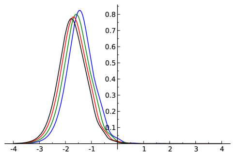
Figure 5: Plots of $L_{+}(x)$ for the connections numerically minimizing $S_{\mathit{YM}}$, with a zero-size instanton at the south pole and a zero-size anti-instanton at the north pole. The bumps move away from the origin as $\min(S_{\mathit{YM}})$ decreases. The graphs of $L_{-}(x)$ are given by the reflection $x\rightarrow-x$.

It seems clear that an instanton is moving towards $x=\infty$ and an anti-instanton towards $x=-\infty$.

Given a widely separated sequence of instantons, $\bar{I}I\bar{I}I$, the symmetry conditions at the enhanced symmetry point force all three of the neighboring pairs to be maximally twisted.

The zero-size limit of such a sequence, $\bar{I}I\bar{I}I$, of instantons and anti-instantons, widely separated in $x$, seems a plausible candidate for the enhanced symmetry fixed point connection with effective index $2$. It seems at least worth trying to check by calculating the Yang-Mills flow on the slow manifold.

It is worrisome that the first numerical minimization did not get closer to $\min(S_{\mathit{YM}})=4$. We would naively expect the sequence of four separated (anti-)instantons to appear quickly, leaving only the sizes as slow modes. Perhaps there is a competing process. Or perhaps there is an error in the computer program. Most likely, the polynomials are not of high enough degree in $t$ to sufficiently resolve the region near $t=\pm 1$.

There is no compelling evidence from the numerical calculations that $\min(S_{\mathit{YM}})=4$ at the enhanced symmetry point. There could still be a smooth fixed point with $S_{\mathit{YM}}<4$, or a hybrid connection containing a zero-size instanton and a zero-size anti-instanton plus a smooth part, with total action $2<S_{\mathit{YM}}<4$. We might note that this could not be the Sibner-Sibner-Uhlenbeck [14] solution of the Yang-Mills equation with $S_{\mathit{YM}}<4$. Their fixed point must have an unstable manifold of dimension $\geq 3$. The Sibner-Sibner-Uhlenbeck construction presupposes a certain $U(1)$ symmetry, and produces a connection with a 1 dimensional unstable manifold in the space of $U(1)$-invariant connections. Any other unstable directions would have to come in doublets of the $U(1)$ symmetry group (two dimensional real representations). So there is no possibility of a two dimensional unstable manifold. A smooth fixed-point must have at least two unstable directions [16], so the Sibner-Sibner-Uhlenbeck connection with $S_{\mathit{YM}}<4$ must have at least 3 unstable directions.

12.2.9 Improved numerical results

The first calculation, described in Section 12.2.6 above, can be re-done with improved resolution near the poles by a trivial modification, simply rescaling $x\rightarrow x/x_{1}$, redefining $t=-\tanh(x/x_{1})$, for appropriate values of $x_{1}$ that are determined empirically. The only change to the computer program is a rescaling of each term in the Yang-Mills action by a power of $x_{1}$.

Some results are shown in Table 4.

$n_{t}$	$n_{s}$	$N$	$x_{1}$	$\min(S_{\mathit{YM}})$
3	5	60	3.0	4.34
4	2	32	3.0	4.17
5	2	40	3.5	4.13
5	5	100	4.0	4.13
6	2	48	4.5	4.08
8	2	64	3.5	4.05
10	2	80	4.0	4.04
12	2	96	4.0	4.04

Table 4: Numerical minimization of $S_{\mathit{YM}}$ with coordinate re-scaling $x\rightarrow x/x_{1}$, choosing $x_{1}$ to obtain the best minimum (roughly).

The evidence for a local minimum at $S_{\mathit{YM}}=4$ is much better. Figure 6

Figure 6: $L_{+}(x)$ for the connection minimizing $S_{\mathit{YM}}$ at $4.04$ with the improved resolution, the last run in Table 4. For comparison, the curve centered at $x=0$ is $L_{+}(x)$ for an instanton.

shows the chiral action density $L_{+}(x)$. Figure 7

Figure 7: $L(x)$ for the connection minimizing $S_{\mathit{YM}}$ at $4.04$ with the improved resolution, the last run in Table 4. The separation into four small (anti-)instantons is more apparent.

shows the full action density $L(x)=L_{+}(x)+L_{-}(x)$. The evidence is stronger for separation into a quadruplet of zero-size (anti-)instantons at the minimum.

12.2.10 A 2-torus family of twisted quadruplets

We write an explicit 2-parameter family of twisted quadruplets of zero-size (anti-)instantons living in the 2-parameter family of bundles constructed in Section 12.2.1 above, parametrized by $(\beta_{1},\beta_{2})\in[0,\pi]^{2}$. Although the family of bundles forms a 2-sphere, the boundary of the square being identified to a point, the 2-parameter family of connections forms a 2-torus, opposite sides of the square being identified with each other.

Write the basic instanton as

$$D_{I}(x-x_{+})=d+\omega-f_{+}\omega\,,\qquad f_{+}=\frac{1}{1+e^{-2(x-x_{+})}}\,.$$ (347)

The basic anti-instanton is

$$D_{\bar{I}}(x-x_{-})=D_{I}(-x+x_{-})\,.$$ (348)

The twisted quadruplet is constructed from an instanton $D_{I}(x-x_{+})$, an anti-instanton $D_{\bar{I}}(x-x_{-})$, and their reflections under $x\rightarrow-x$, the instanton $D_{I}(x+x_{-})=D_{\bar{I}}(-x-x_{-})$, and the anti-instanton $D_{\bar{I}}(x+x_{+})=D_{I}(-x-x_{+})$, in the limit

$$x_{-}\rightarrow\infty\,,\qquad x_{+}-x_{-}\rightarrow\infty$$ (349)

twisted as follows,

$$D(\beta_{1},\beta_{2})=\left\{\begin{array}[]{crrll}\Phi_{-}h_{\beta_{1}}^{-1}D_{\bar{I}}(x+x_{+})h_{\beta_{1}}\Phi_{-}^{-1}&&&x&<-\frac{1}{2}(x_{+}+x_{-})\\ D_{I}(x+x_{-})&&-\frac{1}{2}(x_{+}+x_{-})<&x&<0\\ h_{\beta_{1}}D_{\bar{I}}(x-x_{-})h_{\beta_{1}}^{-1}&&0<&x&<\frac{1}{2}(x_{+}+x_{-})\\ \Phi_{+}D_{I}(x-x_{+})\Phi_{+}^{-1}&&\frac{1}{2}(x_{+}+x_{-})<&x&\end{array}\right.$$ (350)

Recall that the patching map for the bundle is

$$\Phi_{2}(\beta_{1},\beta_{2})=\Phi_{-}^{-1}\Phi_{+}\,,\qquad\Phi_{+}=h_{\beta_{1}}gh_{\beta_{2}}g^{-1}\,,\qquad\Phi_{-}=gh_{\beta_{2}}g^{-1}h_{\beta_{1}}\,.$$ (351)

In the limit, the instantons and anti-instantons agree at the junctions, taking the values

$$D=\left\{\begin{array}[]{crll}gdg^{-1}&&x=-\frac{1}{2}(x_{+}+x_{-})\\ d&&x=0\\ h_{\beta_{1}}gdg^{-1}h_{\beta_{1}}^{-1}&&x=\frac{1}{2}(x_{+}+x_{-})\end{array}\right.$$ (352)

At the north pole, $x=-\infty$,

$$D=\Phi_{-}h_{\beta_{1}}^{-1}dh_{\beta_{1}}\Phi_{-}^{-1}=\Phi_{-}d\Phi_{-}^{-1}$$ (353)

and at the south pole, $x=\infty$,

$$D=\Phi_{+}d\Phi_{+}^{-1}$$ (354)

so $D$ satisfies the boundary conditions defining the bundle. Alternatively, we have connections on the two hemispheres, nonsingular at the poles,

$$D_{-}=\left\{\begin{array}[]{crrll}h_{\beta_{1}}^{-1}D_{\bar{I}}(x+x_{+})h_{\beta_{1}}&&&x&<-\frac{1}{2}(x_{+}+x_{-})\\ \Phi_{-}^{-1}D_{I}(x+x_{-})\Phi_{-}&&-\frac{1}{2}(x_{+}+x_{-})<&x&<0\end{array}\right.$$ (355)

$$D_{+}=\left\{\begin{array}[]{crrll}\Phi_{+}^{-1}h_{\beta_{1}}D_{\bar{I}}(x-x_{-})h_{\beta_{1}}^{-1}\Phi_{+}&&0<&x&<\frac{1}{2}(x_{+}+x_{-})\\ D_{I}(x-x_{+})&&\frac{1}{2}(x_{+}+x_{-})<&x&\end{array}\right.$$ (356)

whose values at $x=0$ are

$$D_{-}=\Phi_{-}^{-1}d\Phi_{-}\,,\qquad D_{+}=\Phi_{+}^{-1}h_{\beta_{1}}dh_{\beta_{1}}^{-1}\Phi_{+}=\Phi_{+}^{-1}d\Phi_{+}$$ (357)

which are related by the patching map defining the bundle

$$D_{-}=\Phi_{2}(\beta_{1},\beta_{2})D_{+}\Phi_{2}(\beta_{1},\beta_{2})^{-1}\,.$$ (358)

So the connection $D(\beta_{1},\beta_{2})$ lives in the bundle defined by the patching map $\Phi_{2}(\beta_{1},\beta_{2})$. Moreover, it can be checked that all the symmetry conditions of the family of bundles are satisfied by the family of connections $D(\beta_{1},\beta_{2})$.

On the boundary of the square, $\beta_{1,2}=0,\pi$, the patching map is trivial, $\Phi_{2}(\beta_{1},\beta_{2})=1$, but the connections $D(\beta_{1},\beta_{2})$ are not all gauge equivalent on the boundary. At $\beta_{1}=0,\pi$,

$$D_{\mp}=\left\{\begin{array}[]{crrll}D_{\bar{I}}(x+x_{+})&&&x&<-\frac{1}{2}(x_{+}+x_{-})\\ \left(gh_{\beta_{2}}g^{-1}\right)^{-1}D_{I}(x+x_{-})\left(gh_{\beta_{2}}g^{-1}\right)&&-\frac{1}{2}(x_{+}+x_{-})<&x&<0\\ \left(gh_{\beta_{2}}g^{-1}\right)^{-1}D_{\bar{I}}(x-x_{-})\left(gh_{\beta_{2}}g^{-1}\right)&&0<&x&<\frac{1}{2}(x_{+}+x_{-})\\ D_{I}(x-x_{+})&&\frac{1}{2}(x_{+}+x_{-})<&x&\end{array}\right.$$ (359)

At $\beta_{2}=0,\pi$,

$$D_{\mp}=\left\{\begin{array}[]{crrll}h_{\beta_{1}}^{-1}D_{\bar{I}}(x+x_{+})h_{\beta_{1}}&&&x&<-\frac{1}{2}(x_{+}+x_{-})\\ h_{\beta_{1}}^{-1}D_{I}(x+x_{-})h_{\beta_{1}}&&-\frac{1}{2}(x_{+}+x_{-})<&x&<0\\ D_{\bar{I}}(x-x_{-})&&0<&x&<\frac{1}{2}(x_{+}+x_{-})\\ D_{I}(x-x_{+})&&\frac{1}{2}(x_{+}+x_{-})<&x&\end{array}\right.$$ (360)

The boundary of the square cannot be identified to a single point to give a 2-sphere family of connections. Rather, the opposite sides of the square are identified, giving a 2-torus family of connections, as might have been expected from the symmetry conditions on the family.

It remains to calculate the Y-M flow near this family of connections, first to check that the connection at the enhanced symmetry point $\beta_{1}=\beta_{2}=\frac{\pi}{2}$ has a two-dimensional unstable manifold, then to trace the global shape of that 2-manifold. We see two possibilities, depending on details of the flow on the slow manifold, yet to be calculated. The 2-torus of twisted quadruplets could be connected to the flat connection by a single outgoing trajectory leaving from the distinguished point $(\beta_{1},\beta_{2})=(0,0)$ (identified with the other 3 corners of the square). This outgoing trajectory in $\mathcal{A}/\mathcal{G}$ would lift to a 2-cylinder in $\mathcal{A}$, each point on the trajectory in $\mathcal{A}/\mathcal{G}$ lifting to a nontrivial loop in the group of gauge transformations, $\mathcal{G}$. In this scenario, the Y-M flow would have a stable 2-torus of zero area which might, in the lambda model, produce non-canonical low energy interactions in $SU(2)$ gauge theory. A second, less attractive, scenario would have outgoing trajectories leaving from each point on the boundary of the square, travelling to the flat connection. The unstable manifold would form a 2-sphere stable under the Y-M flow, with non-zero area.

13 Questions and comments

13.1 Does the outgoing trajectory end at the flat connection?

The topology of the Y-M flow is the same whatever the locations of the twisted pair in $S^{4}$ and whatever the geometry on $S^{4}$. There is always an outgoing trajectory from the aligned twisted pair. Does that outgoing trajectory always end at the flat connection?

Euclidean $\mathbb{R}^{4}$ is the setting of interest for the possible physics application (discussed in section 13.3 below). The twisted pair in euclidean $\mathbb{R}^{4}$ can be obtained as the limit of twisted pairs in $S^{4}$ in which the instanton and anti-instanton are brought together while the metric on $S^{4}$ is scaled so that the distance of separation remains constant. Scaling the metric on $S^{4}$ is equivalent to scaling the Y-M flow time, so the outgoing trajectory for twisted pairs in $\mathbb{R}^{4}$ is the same as the limiting trajectory for twisted pairs in $S^{4}$ as the instanton and anti-instanton approach each other. Even if the outgoing trajectory ends at the flat connection for all twisted pairs in $S^{4}$, there would still remain the possibility of cross-over to another fixed point as the locations of the instanton and anti-instanton approach each other, which would govern the outgoing trajectory for twisted pairs in $\mathbb{R}^{4}$. Does such a cross-over take place? or does the outgoing trajectory end at the flat connection for twisted pairs in euclidean $\mathbb{R}^{4}$?

Whatever the fixed point at the end of the outgoing trajectory, it will have $S_{\mathit{YM}}<2$, so it cannot be singular. If it is not the flat connection, then Taubes’ theorem [16] says it must have at least a two dimensional unstable manifold. It would seem extraordinary for the outgoing trajectory from the twisted pairs to end exactly on a twice unstable fixed point.

13.2 Asymptotic behavior of the outgoing trajectory?

For the possible application to physics, we would like to know how the outgoing trajectory approaches the flat connection at large time, especially for twisted pairs in euclidean $\mathbb{R}^{4}$ (presuming the outgoing trajectory does end at the flat connection). Near its end, the trajectory $A_{t}$ will approach the flat connection as a decaying perturbation whose Fourier transform in $\mathbb{R}^{4}$ takes the form

$$\tilde{A}_{t}(p)=e^{-tp^{2}}\tilde{A}_{0}(p)\,.$$ (361)

The amplitudes $\tilde{A}_{0}(p)$ will depend on the locations and twist of the twisted pair and will presumably control the observable properties of the hypothetical physical states associated with the twisted pair.

We might explore for clues to the outgoing trajectories by looking at the outgoing trajectory for the $U(2)$-invariant twisted pair on $S^{4}$, given by equation 229,

$$\frac{df}{dt}=R^{2}(x)^{-1}\left[\partial_{x}^{2}f+4f(1-f)(2f-1)\right]=(\cosh x)^{2}\left[\partial_{x}^{2}f+4f(1-f)(2f-1)\right]\,.$$ (362)

The flow equation for the outgoing trajectory in the slow manifold is given by equation 214 at $\sigma=0$ or $\sigma=2\pi$,

$$\frac{d\rho}{dt}=3\rho^{3}\,.$$ (363)

It determines the asymptotic initial conditions in the far past, $t\rightarrow-\infty$, for the outgoing trajectory,

$$f_{t}(x)\rightarrow f_{+}(|x|)\,,\qquad f_{+}(x)=\frac{1}{1+e^{-2(x-x_{+}(t))}}\,,\qquad x_{+}(t)=\frac{1}{2}\ln(-6t)+O(t^{-1})\,.$$ (364)

If, instead of the round metric on $S^{4}$, we were to use the cylindrical metric, $R^{2}(x)=1$, the outgoing trajectory would be given by

$$\frac{df}{dt}=\partial_{x}^{2}f+4f(1-f)(2f-1)$$ (365)

which is a nonlinear diffusion or reaction-diffusion equation known as the Newell-Whitehead-Segel equation, a special case of the Kolmogorov-Petrovsky-Piskounov/FitzHugh-Nagumo equation. It is apparently not integrable, but some exact solutions are known (see for example [33]). Given the asymptotic $t\rightarrow-\infty$ conditions we need for the outgoing trajectory, the methods by which the exact solutions were produced do not seem applicable [34]. Still, the possibility of an exact solution for the outgoing trajectory is tantalizing.

For twisted pairs in $\mathbb{R}^{4}$, the only symmetry of the outgoing trajectory is the $SO(3)$ group of rotations around the axis that passes through the locations of the instanton and anti-instanton. The unstable trajectory is given by a set of nonlinear diffusion equations in two spatial dimensions. Numerical integration might be the only way to find its long time asymptotic behavior.

13.3 The lambda model

The lambda model [7] is a two-dimensional nonlinear model whose target space is the manifold of spacetime fields: gauge fields, fermion fields, scalar fields, and the spacetime metric of general relativity. The functional integral of the lambda model is

$$\int\mathcal{D}\lambda\;\exp\left[{-\int d^{2}z\;\frac{1}{g^{2}}G_{ij}(\lambda)\partial\lambda^{i}\bar{\partial}\lambda^{j}}\right]$$ (366)

$$\mathcal{D}\lambda=\prod_{z,\bar{z}}d\rho(\lambda(z,\bar{z}))\,.$$ (367)

The field $\lambda(z,\bar{z})$ maps a two-dimensional domain, parametrized by a complex coordinate $z$, to the manifold of spacetime fields. The $\lambda^{i}$ are coordinates on the manifold of spacetime fields (e.g., their momentum modes), $G_{ij}(\lambda)d\lambda^{i}d\lambda^{j}$ is the natural metric on the manifold of spacetime fields, $g$ is the coupling constant, and $d\rho(\lambda)$ is a measure on the spacetime fields, the a priori measure of the nonlinear model. The lambda model differs from the standard two dimensional nonlinear model in that the fields $\lambda^{i}(z,\bar{z})$ are not precisely dimensionless, but change with the two-dimensional scale $\Lambda$ according to the gradient flow

$$\Lambda\frac{\partial\hfill}{\partial\Lambda}\lambda^{i}=-\nabla^{i}S(\lambda)\,,\qquad\nabla^{i}S=g^{2}G^{ij}\frac{\partial\hfill}{\partial\lambda^{j}}\left(\frac{1}{g^{2}}S\right)$$ (368)

where $\frac{1}{g^{2}}S$ is the classical action functional of the spacetime field theory. For small fluctuations, the dimension of the mode $\lambda^{i}$ is $p(i)^{2}$ where $p(i)$ is the spacetime momentum of the mode.

The a priori measure is produced by the fluctuations of the lambda fields at short 2-d distances, acting in combination with the gradient flow. The mechanism of production is expressed by the renormalization group equation for the a priori measure, which at leading order is the driven diffusion equation

$$\Lambda\frac{\partial\hfill}{\partial\Lambda}d\rho=\nabla_{i}\,g^{2}G^{ij}\left[\nabla_{j}+\partial_{j}\left(\frac{1}{g^{2}}S\right)\right]d\rho$$ (369)

which equilibrates at

$$d\rho=d\lambda\;e^{-\frac{1}{g^{2}}S}\,,$$ (370)

$d\lambda$ being the metric volume element. We recognize the a priori measure produced by the small fluctuations as the functional measure of the canonically quantized spacetime quantum field theory.

The exact a priori measure produced by the lambda model is a quantum field theory in spacetime that might not be identical to the canonically quantized field theory. We are pursuing the possibility that non-canonical corrections to the canonical quantum field theory might be produced by large two-dimensional fluctuations in the lambda model. At weak coupling, large fluctuations in a nonlinear model show up as winding modes, associated with $\pi_{1}$ of the target manifold, and as 2-d instantons, associated with $\pi_{2}$ of the target manifold. The winding modes might provide weakly interacting states not present in the canonical quantum $SU(2)$ gauge field theory. The 2-d instantons might provide interactions not present in the canonical quantum $SU(2)$ and $SU(3)$ gauge field theories.

The evolution of the nonlinear model in the two dimensional scale can be represented by the radial quantization, in which the wave functions live on the loop space of the target manifold and the hamiltonian is the 2-d dilation operator. The dilation operator of the lambda model is the ordinary dilation operator of the nonlinear model combined with the gradient flow. The winding modes are wave functions on the nontrivial component(s) of the loop space. In a normal nonlinear model, the low-lying winding modes are concentrated on the nontrivial loops of minimal length. In the lambda model, the gradient flow attempts to concentrate the wave function on the stable nontrivial loops. The two processes compete, in principle, so searching only for loops stable under the gradient flow was ill-conceived. Finding a stable loop of zero length was pure luck.

It remains to quantize the stable loop of $SU(2)$ gauge fields. The ground state or states will be concentrated on the nontrivial loop at the tip of the cone in Figure 2. Regarding the cone as an orbifold of the plane, the states of the stable loop are the twist states for the orbifold. The classical ground state energy is zero because the length of the loop is zero. But, if the stable loop is to provide any low energy states, the quantum corrections to the ground state energy must also vanish, at least to many orders in the coupling constant. We assume a high fundamental spacetime energy scale in the lambda model. Fermion zero-modes localized in the zero-size instanton and anti-instanton of the stable loop will provide degenerate ground states that offers at least a possibility of canceling the quantum corrections to the ground state energy, but to get cancellation to many orders or to all orders, we will probably need perturbative spacetime supersymmetry. The hypothetical non-canonical $SU(2)$ gauge theory states would only be visible at low energy in theories with perturbative supersymmetry.

It also remains to figure out the spacetime interpretation of the states of the stable loop. Do they appear as additional fields in the quantum field theory, or as extra states, in addition to the quantum field theory? In any case, they will presumably be bi-local objects, depending on the two instanton locations parametrizing the loop of twisted pairs.

For consistency in the 2-d quantum field theory, twist fields have to be accompanied by a projection that eliminates all states with nontrivial monodromy around the twist field. Here, nontrivial monodromy means change of sign under nontrivial $SU(2)$ gauge transformations. Such states arise in canonically quantized gauge theories that have a global $SU(2)$ anomaly [35]. By projecting out the anomalous states, and adding new non-canonical states, the lambda model might produce a non-anomalous quantization of such gauge theories.

We expect that interactions with the ordinary modes of the gauge field theory will be determined by the outgoing trajectory that leads from the twisted pairs to the flat connection. We picture two twist fields — two loops of twisted pairs — merging in the two dimensional domain. Any closed curve surrounding them will be a topologically trivial loop in the twisted pairs. In the radial quantization, it will be driven down the outgoing trajectory to the flat connection, where it can join to the rest of the two dimensional domain where there are only small fluctuations around the flat connection. The interactions of the new states associated with the stable loop should then be determined by how the outgoing trajectory approaches the flat connection.

We picture a 2-d instanton in the lambda model to consist of a point-like core that is the nontrivial 2-sphere of twisted pairs of $SU(3)$ gauge fields (or twisted quadruplets of $SU(2)$ gauge fields), evolving outwards in the radial quantization, down the outgoing trajectory towards the flat connection. Again, the effects on the ordinary states will be determined by how the outgoing trajectory approaches the flat connection. On the two dimensional domain, the instanton will look like a defect, around which the nearly flat gauge field winds by a nontrivial loop in the group of gauge transformations.

So far, we have only such vague speculations. The task now is to figure out how to calculate in the lambda model with the stable loop and the stable 2-spheres of gauge fields.

Appendix A $U(2)$-invariant connections on $S^{4}$

A.1 $S^{3}$, $SU(2)$, $U(2)$, $SO(4)$, $S^{4}$

$S^{3}$:

$$\mathbf{z}=\begin{pmatrix}z_{1}\\ z_{2}\end{pmatrix}\,,\qquad\mathbf{z}^{\dagger}\mathbf{z}=\bar{z}_{1}z_{1}+\bar{z}_{2}z_{2}=1\,,\qquad P(\mathbf{z})=\mathbf{z}\mathbf{z}^{\dagger}\,,\qquad Q(\mathbf{z})=1-P(\mathbf{z})\,,$$ (371)

$$\mathrm{dvol}_{S^{3}}=-\frac{1}{2}(\mathbf{z}^{\dagger}d\mathbf{z})(d\mathbf{z}^{\dagger}d\mathbf{z})\,,\qquad\int_{S^{3}}\mathrm{dvol}_{S^{3}}=2\pi^{2}\,.$$ (372)

$SU(2)$:

$$g(\mathbf{z})=\begin{pmatrix}z_{1}&-\bar{z}_{2}\\ z_{2}&\bar{z}_{1}\end{pmatrix}\,.$$ (373)

$U(2)$:

$$g(U\mathbf{z})=Ug(\mathbf{z})\begin{pmatrix}1&0\\ 0&(\det U)^{-1}\end{pmatrix}\,.$$ (374)

$SO(4)=SU(2)\times SU(2)/\mathbb{Z}_{2}$:

$$g(O(\mathbf{z}))=g_{L}g(\mathbf{z})g_{R}^{-1}\,.$$ (375)

$S^{4}$:

$$\vec{y}=(\cos\theta,\mathbf{z}\sin\theta)\,,\qquad x=\ln\tan\left(\frac{\theta}{2}\right)\,,\qquad-\infty\leq x\leq\infty\,.$$ (376)

$$(ds)_{S^{4}}^{2}=R^{2}(x)\left[(dx)^{2}+d\mathbf{z}^{\dagger}d\mathbf{z}\right]\,,\qquad R^{2}(x)=(\cosh x)^{-2}\,.$$ (377)

A.2 $U(2)$-invariant $su(2)$-valued 1-forms on $S^{3}$

$$\eta =-PdP =-(\mathbf{z}^{\dagger}d\mathbf{z})\mathbf{z}\mathbf{z}^{\dagger}-\mathbf{z}d\mathbf{z}^{\dagger}$$ (378)

$$\eta^{\dagger} =-dPP =(\mathbf{z}^{\dagger}d\mathbf{z})\mathbf{z}\mathbf{z}^{\dagger}-d\mathbf{z}\mathbf{z}^{\dagger}$$ (379)

$$\eta_{3} =(\mathbf{z}^{\dagger}d\mathbf{z})(P-Q) =(\mathbf{z}^{\dagger}d\mathbf{z})(2\mathbf{z}\mathbf{z}^{\dagger}-1)$$ (380)

$$\eta(\mathbf{e})=\begin{pmatrix}0&-d\bar{z}_{2}\\ 0&0\end{pmatrix}\qquad\eta^{\dagger}(\mathbf{e})=\begin{pmatrix}0&0\\ -dz_{2}&0\end{pmatrix}\qquad\eta_{3}(\mathbf{e})=\begin{pmatrix}dz_{1}&0\\ 0&-dz_{1}\end{pmatrix}$$ (381)

$$\eta^{2}=(\eta^{\dagger})^{2}=\eta_{3}^{2}=0$$ (382)

$$d_{\omega}\omega=d\omega+\{\omega,\,\omega\}=\omega^{2}$$ (383)

$$d_{\omega}(-\eta+\eta^{\dagger}-\eta_{3})=\{\eta_{3},\eta\}-\{\eta_{3},\eta^{\dagger}\}-\{\eta,\eta^{\dagger}\}$$ (384)

so, by $U(1)$-covariance,

$$d_{\omega}\eta=-\{\eta_{3},\eta\}\qquad d_{\omega}\eta^{\dagger}=-\{\eta_{3},\eta^{\dagger}\}\qquad d_{\omega}\eta_{3}=\{\eta,\eta^{\dagger}\}$$ (385)

A.3 $U(2)$-invariant $su(2)$-valued 2-forms on $S^{3}$

Define

$$\sigma =\frac{1}{2}d_{\omega}\eta =-\frac{1}{2}\{\eta_{3},\,\eta\} =\mathbf{z}^{\dagger}d\mathbf{z}PdP =-\mathbf{z}^{\dagger}d\mathbf{z}\,\eta$$ (386)

$$\sigma^{\dagger} =\frac{1}{2}d_{\omega}\eta^{\dagger} =-\frac{1}{2}\{\eta_{3},\,\eta^{\dagger}\} =-\mathbf{z}^{\dagger}d\mathbf{z}dPP =\mathbf{z}^{\dagger}d\mathbf{z}\,\eta^{\dagger}$$ (387)

$$\sigma_{3} =\frac{1}{2}d_{\omega}\eta_{3} =\frac{1}{2}\{\eta,\,\eta^{\dagger}\} =\frac{1}{2}(dP)^{2} =\frac{1}{2}d\mathbf{z}^{\dagger}d\mathbf{z}(P-Q)$$ (388)

$$\sigma(\mathbf{e})=\begin{pmatrix}0&dz_{1}d\bar{z}_{2}\\ 0&0\end{pmatrix}\qquad\sigma^{\dagger}(\mathbf{e})=\begin{pmatrix}0&0\\ d\bar{z}_{1}dz_{2}&0\end{pmatrix}\qquad\sigma_{3}(\mathbf{e})=\frac{1}{2}d\bar{z}_{2}dz_{2}\begin{pmatrix}1&0\\ 0&-1\end{pmatrix}$$ (389)

A.4 $U(2)$-invariant $su(2)$-valued forms on $S^{4}$

The volume form on $S^{3}$ is

$$\mathrm{dvol}_{S^{3}}(\mathbf{e})=-\frac{1}{2}dz_{1}d\bar{z}_{2}dz_{2}\qquad\mathrm{dvol}_{S^{3}}=-\frac{1}{2}(\mathbf{z}^{\dagger}d\mathbf{z})(d\mathbf{z}^{\dagger}d\mathbf{z})\qquad\int_{S^{3}}\mathrm{dvol}_{S^{3}}=2\pi^{2}\,.$$ (390)

In $S^{4}$, at each $x$, we have a basis for the $U(2)$-invariant $su(2)$-valued forms

0-forms: $$i(P-Q)\,,$$ (391)

1-forms: $$idx(P-Q)\,,\eta\,,\eta^{\dagger}\,,\eta_{3}\,,\hfill$$ (392)

2-forms: $$\sigma\,,\sigma^{\dagger}\,,\sigma_{3}\,,dx\,\eta\,,dx\,\eta^{\dagger}\,,dx\,\eta_{3}\,,$$ (393)

3-forms: $$i\mathrm{dvol}_{S^{3}}(P-Q)\,,dx\,\sigma\,,dx\,\sigma^{\dagger}\,,dx\,\sigma_{3}\,.$$ (394)

A.5 Hodge $*$

At $(x,\mathbf{e})\in S^{4}$, the Hodge $*$ operator acts on

1-forms and 3-forms:

$${*}^{2} =-1\qquad {*}dx =R^{2}(x)\mathrm{dvol}_{S^{3}}\qquad {*}dz_{1} =-R^{2}(x)dxd\bar{z}_{2}dz_{2}$$ (395)

$${*}dz_{2} =-R^{2}(x)dxdz_{1}dz_{2}\quad \quad{*}d\bar{z}_{2} =R^{2}(x)dxdz_{1}d\bar{z}_{2}$$ (396)

2-forms:

$${*}^{2}=1\qquad{*}(dxdz_{1})=\frac{1}{2}d\bar{z}_{2}dz_{2}\qquad{*}(dxdz_{2})=dz_{1}dz_{2}\qquad{*}(dxd\bar{z}_{2})=-dz_{1}d\bar{z}_{2}$$ (397)

So Hodge ${*}$ acts on the $U(2)$-invariant $su(2)$-valued forms by:

1-forms and 3-forms:

$${*}idx(P-Q)=R^{2}(x)\mathrm{dvol}_{S^{3}}i(P-Q)$$ (398)

$${*}\eta=-R^{2}(x)dx\sigma\qquad{*}\eta^{\dagger}=-R^{2}(x)dx\sigma^{\dagger}\qquad{*}\eta_{3}=-R^{2}(x)dx\sigma_{3}$$ (399)

2-forms:

$${*}(dx\eta)=\sigma\qquad{*}(dx\eta^{\dagger})=\sigma^{\dagger}\qquad{*}(dx\eta_{3})=\sigma_{3}$$ (400)

A.6 $F$, $F_{\pm}$

Recall

$$d+A=d_{\omega}+\Delta A$$ (401)

$$\Delta A=f(x)\eta-\bar{f}(x)\eta^{\dagger}+f_{3}(x)\eta_{3}\,,\qquad f_{3}=\bar{f}_{3}$$ (402)

$$F=(d_{\omega}+\Delta A)^{2}=d_{\omega}\Delta A+(\Delta A)^{2}$$ (403)

$$F_{\pm}=\frac{1}{2}(1\pm{*})F\,.$$ (404)

Calculate

$$F=\partial_{x}fdx\eta-\partial_{x}\bar{f}dx\eta^{\dagger}+\partial_{x}f_{3}dx\eta_{3}+2f\sigma-2\bar{f}\sigma^{\dagger}+2f_{3}\sigma_{3}-2f_{3}f\sigma+2f_{3}\bar{f}\sigma^{\dagger}-2f\bar{f}\sigma_{3}$$ (405)

$$F_{\pm} =[\partial_{x}f\pm 2(1-f_{3})f)]\,\frac{1}{2}(1\pm{*})dx\eta-[\partial_{x}\bar{f}\pm 2(1-f_{3})\bar{f})]\,\frac{1}{2}(1\pm{*})dx\eta^{\dagger}$$ (406)

$$\quad{}+[\partial_{x}f_{3}\pm 2(f_{3}-f\bar{f})]\,\frac{1}{2}(1\pm{*})dx\eta_{3}$$ (407)

A.7 $L_{\pm}$

$$\frac{1}{4}\mathrm{tr}(-F_{\pm}{*}F_{\pm})=\mp\frac{1}{4}\mathrm{tr}(F_{\pm}^{2})=L_{\pm}(x)dx\,\mathrm{dvol}_{S^{3}}$$ (408)

$$\mp\frac{1}{4}\mathrm{tr}(F_{\pm}^{2}) =\mp\frac{1}{4}\left[\partial_{x}f_{3}\pm 2\left(f_{3}-|f|^{2}\right)\right]^{2}\,\frac{1}{2}\mathrm{tr}(\pm dx\eta_{3}\sigma_{3})$$ (409)

$$\qquad{}\mp\frac{1}{4}\left|\partial_{x}f\pm 2\left(1-f_{3}\right)f)\right|^{2}\,\frac{1}{2}\mathrm{tr}(\mp dx\eta\sigma^{\dagger}\mp dx\eta^{\dagger}\sigma)$$

$$=\frac{1}{4}\left[\partial_{x}f_{3}\pm 2\left(f_{3}-|f|^{2}\right)\right]^{2}dx\,\mathrm{dvol}_{S^{3}}+\frac{1}{2}\left|\partial_{x}f\pm 2\left(1-f_{3}\right)f)\right|^{2}dx\,\mathrm{dvol}_{S^{3}}$$ (410)

$$L_{\pm}=\frac{1}{4}\left[\partial_{x}f_{3}\pm 2\left(f_{3}-|f|^{2}\right)\right]^{2}+\frac{1}{2}\left|\partial_{x}f\pm 2\left(1-f_{3}\right)f)\right|^{2}$$ (411)

A.8 Products of 1-forms and 2-forms

The nonzero products of 1-forms and 2-forms are

$$\sigma\eta^{\dagger}=\eta\sigma^{\dagger}=2\mathrm{dvol}_{S^{3}}P\qquad\sigma^{\dagger}\eta=\eta^{\dagger}\sigma=2\mathrm{dvol}_{S^{3}}Q\qquad\eta_{3}\sigma_{3}=\sigma_{3}\eta_{3}=-\mathrm{dvol}_{S^{3}}\mathbf{1}$$ (412)

So

$$[\omega,\,\sigma]=[\omega,\,\sigma^{\dagger}]=-2\mathrm{dvol}_{S^{3}}(P-Q)\qquad[\omega,\,\sigma_{3}]=0$$ (413)

A.9 Inner products

The non-zero inner products are:

1-forms:

$$\mathrm{tr}\left[-idx(P-Q){*}idx(P-Q)\right]=\mathrm{tr}\left(\eta{*}\eta^{\dagger}\right)=\mathrm{tr}\left(\eta^{\dagger}{*}\eta\right)=\mathrm{tr}\left(-\eta_{3}{*}\eta_{3}\right)=2R^{2}(x)dx\mathrm{dvol}_{S^{3}}$$ (414)

2-forms:

$$\mathrm{tr}(-dx\eta_{3}\sigma_{3})=\mathrm{tr}(dx\eta\sigma^{\dagger})=\mathrm{tr}(dx\eta^{\dagger}\sigma)=2dx\,\mathrm{dvol}_{S^{3}}$$ (415)

A.10 New basis for the $U(2)$-invariant forms

Change basis for the $U(2)$-invariant $su(2)$-valued 1-forms and 2-forms on $S^{3}$ to

$$\omega =-\eta+\eta^{\dagger}-\eta_{3}\qquad \omega_{1} =\eta-\eta^{\dagger}-2\eta_{3}\qquad \omega_{2} =-i(\eta+\eta^{\dagger})$$ (416)

$$\chi =-\sigma+\sigma^{\dagger}-\sigma_{3} \chi_{1} =\sigma-\sigma^{\dagger}-2\sigma_{3} \chi_{2} =-i(\sigma+\sigma^{\dagger})$$ (417)

Correspondingly, on $S^{4}$,

1-forms: $$idx(P-Q)\,,\omega\,,\omega_{1}\,,\omega_{2}\hfill$$ (418)

2-forms: $$\chi\,,\chi_{1}\,,\chi_{2}\,,$$ (419)

$$dx\,\omega\,,dx\,\omega_{1}\,,dx\,\omega_{2}$$ (420)

3-forms: $$i\mathrm{dvol}_{S^{3}}(P-Q)\,,dx\,\chi\,,dx\,\chi_{1}\,,dx\,\chi_{2}\,.$$ (421)

A.11 Formulas in the new basis

$$d_{\omega}\omega =2\chi d_{\omega}\omega_{1} =2\chi_{1} d_{\omega}\omega_{2} =2\chi_{2}$$ (422)

$$\{\omega,\,\omega\} =4\chi \{\omega,\,\omega_{1}\} =-2\chi_{1} \{\omega,\,\omega_{2}\} =2\chi_{2}$$ (423)

$$D_{\pm}\omega =(2-4f_{\pm})\chi\quad D_{\pm}\omega_{1} =(2+2f_{\pm})\chi_{1}\quad D_{\pm}\omega_{2} =(2-2f_{\pm})\chi_{2}$$ (424)

$$[\omega,\,\chi]=[\omega,\,\chi_{1}]=0\qquad[\omega,\,\chi_{2}]=4i\mathrm{dvol}_{S^{3}}(P-Q)$$ (425)

Hodge ${*}$ on 1-forms:

$${*}idx(P-Q)=R^{2}(x)\mathrm{dvol}_{S^{3}}i(P-Q)$$ (426)

$${*}\omega=-R^{2}(x)dx\chi\qquad{*}\omega_{1}=-R^{2}(x)dx\chi_{1}\qquad{*}\omega_{2}=-R^{2}(x)dx\chi_{2}$$ (427)

Hodge ${*}$ on 2-forms:

$${*}\chi=dx\omega\qquad{*}\chi_{1}=dx\omega_{1}\qquad{*}\chi_{2}=dx\omega_{2}$$ (428)

Non-zero inner products of 1-forms:

$$\mathrm{tr}\left[-idx(P-Q){*}idx(P-Q)\right]=2R^{2}(x)dx\mathrm{dvol}_{S^{3}}$$ (429)

$$\frac{1}{6}\mathrm{tr}(-\omega{*}\omega)=\frac{1}{8}\mathrm{tr}(-\omega_{1}{*}\omega_{1})=\frac{1}{4}\mathrm{tr}(-\omega_{2}{*}\omega_{2})=R^{2}(x)dx\mathrm{dvol}_{S^{3}}$$ (430)

Non-zero inner products of 2-forms:

$$\frac{1}{6}\mathrm{tr}(-dx\omega{*}dx\omega)=\frac{1}{8}\mathrm{tr}(-dx\omega_{1}{*}dx\omega_{1})=\frac{1}{4}\mathrm{tr}(-dx\omega_{2}{*}dx\omega_{2})=dx\mathrm{dvol}_{S^{3}}$$ (431)

A.12 Instanton covariant derivatives

Using the formulas in Appendix A.2, we calculate the instanton covariant derivatives of the 1-forms

$$D_{\pm}idx(P-Q)=-2f_{\pm}dx\omega_{2}\qquad D_{\pm}\omega=\lambda\chi\qquad D_{\pm}\omega_{1}=\lambda_{1}\chi_{1}\qquad D_{\pm}\omega_{2}=\lambda_{2}\chi_{2}$$ (432)

where

$$\lambda=2(1-2f_{\pm})\qquad\lambda_{1}=2(1+f_{\pm})\qquad\lambda_{2}=2(1-f_{\pm})\,.$$ (433)

The covariant derivatives of the 2-forms are

$$D_{\pm}(dx\,\omega)=-\lambda dx\,\chi\qquad D_{\pm}(dx\,\omega_{1})=-\lambda_{1}dx\,\chi_{1}\qquad D_{\pm}(dx\,\omega_{2})=-\lambda_{2}dx\,\chi_{2}$$ (434)

$$D_{\pm}\chi=0\qquad D_{\pm}\chi_{1}=0\qquad D_{\pm}\chi_{2}=-4f_{\pm}\mathrm{dvol}_{S^{3}}i(P-Q)$$ (435)

Their Hodge duals are

$${*}D_{\pm}(dx\,\omega)=-R^{2}(x)^{-1}\lambda\omega\qquad{*}D_{\pm}(dx\,\omega_{1})=-R^{2}(x)^{-1}\lambda_{1}\omega_{1}$$ (436)

$${*}D_{\pm}(dx\,\omega_{2})=-R^{2}(x)^{-1}\lambda_{2}\omega_{2}$$ (437)

$${*}D_{\pm}\chi=0\qquad{*}D_{\pm}\chi_{1}=0\qquad{*}D_{\pm}\chi_{2}=4R^{2}(x)^{-1}f_{\pm}idx(P-Q)$$ (438)

A.13 The instanton laplacian

$$D_{\pm}\delta A_{0\pm}(x)idx(P-Q) =-\delta A_{0\pm}2f_{\pm}dx\omega_{2}$$ (439)

$$({*}\mp 1)D_{\pm}\delta A_{0\pm}(x)idx(P-Q) =-2f_{\pm}\delta A_{0\pm}(\chi_{2}\mp dx\omega_{2})$$ (440)

$$D_{\pm}({*}\mp 1)D_{\pm}\delta A_{0\pm}(x)idx(P-Q) =-2\partial_{x}(f_{\pm}\delta A_{0\pm})dx\chi_{2}-2f_{\pm}\delta A_{0\pm}(D_{\pm}\chi_{2}\mp D_{\pm}dx\omega_{2})$$ (441)

$${*}D_{\pm}({*}\mp 1)D_{\pm}\delta A_{0\pm}(x)idx(P-Q) =-2\partial_{x}(f_{\pm}\delta A_{0\pm})R^{2}(x)^{-1}\omega_{2}$$ (442)

$$\qquad{}-2f_{\pm}\delta A_{0\pm}\left[4R^{2}(x)^{-1}f_{\pm}idx(P-Q)\right.$$ (443)

$$\qquad\qquad\qquad\qquad\qquad{}\left.\mp(-\lambda_{2})R^{2}(x)^{-1}\omega_{2}\right]$$ (444)

$$=-2R^{2}(x)^{-1}(\partial_{x}\pm\lambda_{2})(f_{\pm}\delta A_{0\pm})\omega_{2}$$ (445)

$$\qquad{}-8R^{2}(x)^{-1}f_{\pm}^{2}\delta A_{0\pm}idx(P-Q)$$ (446)

$$D_{\pm}\delta f_{\pm}(x)\omega =\partial_{x}\delta f_{\pm}dx\omega+\delta f_{\pm}\lambda\chi$$ (447)

$$({*}\mp 1)D_{\pm}\delta f_{\pm}(x)\omega =(\partial_{x}\mp\lambda)\delta f_{\pm}(\chi\mp dx\omega)$$ (448)

$$D_{\pm}({*}\mp 1)D_{\pm}\delta f_{\pm}(x)\omega =\partial_{x}(\partial_{x}\mp\lambda)\delta f_{\pm}dx\chi+(\partial_{x}\mp\lambda)\delta f_{\pm}(D_{\pm}\chi\mp D_{\pm}dx\omega)$$ (449)

$${*}D_{\pm}({*}\mp 1)D_{\pm}\delta f_{\pm}(x)\omega =R^{2}(x)^{-1}(\partial_{x}\pm\lambda)(\partial_{x}\mp\lambda)\delta f_{\pm}\omega$$ (450)

$$D_{\pm}\delta A_{1\pm}(x)\omega_{1} =\partial_{x}\delta A_{1\pm}dx\omega_{1}+\delta A_{1\pm}\lambda_{1}\chi_{1}$$ (451)

$$({*}\mp 1)D_{\pm}\delta A_{1\pm}(x)\omega_{1} =(\partial_{x}\mp\lambda_{1})\delta A_{1\pm}(\chi_{1}\mp dx\omega_{1})$$ (452)

$$D_{\pm}({*}\mp 1)D_{\pm}\delta A_{1\pm}(x)\omega_{1} =\partial_{x}(\partial_{x}\mp\lambda_{1})\delta A_{1\pm}dx\chi_{1}+(\partial_{x}\mp\lambda_{1})\delta A_{1\pm}(D_{\pm}\chi_{1}\mp D_{\pm}dx\omega_{1})$$ (453)

$${*}D_{\pm}({*}\mp 1)D_{\pm}\delta A_{1\pm}(x)\omega_{1} =R^{2}(x)^{-1}(\partial_{x}\pm\lambda_{1})(\partial_{x}\mp\lambda_{1})\delta A_{1\pm}\omega_{1}$$ (454)

$$D_{\pm}\delta A_{2\pm}(x)\omega_{2} =\partial_{x}\delta A_{2\pm}dx\omega_{2}+\delta A_{2\pm}\lambda_{2}\chi_{2}$$ (455)

$$({*}\mp 1)D_{\pm}\delta A_{2\pm}(x)\omega_{2} =(\partial_{x}\mp\lambda_{2})\delta A_{2\pm}(\chi_{2}\mp dx\omega_{2})$$ (456)

$$D_{\pm}({*}\mp 1)D_{\pm}\delta A_{2\pm}(x)\omega_{2} =\partial_{x}(\partial_{x}\mp\lambda_{2})\delta A_{2\pm}dx\chi_{2}+(\partial_{x}\mp\lambda_{2})\delta A_{2\pm}(D_{\pm}\chi_{2}\mp D_{\pm}dx\omega_{2})$$ (457)

$${*}D_{\pm}({*}\mp 1)D_{\pm}\delta A_{2\pm}(x)\omega_{2} =\partial_{x}(\partial_{x}\mp\lambda_{2})\delta A_{2\pm}R^{2}(x)^{-1}\omega_{2}$$ (458)

$$\qquad{}+(\partial_{x}\mp\lambda_{2})\delta A_{2\pm}(4R^{2}(x)^{-1}f_{\pm}idx(P-Q)\pm R^{2}(x)^{-1}\lambda_{2}\omega_{2})$$

$${*}D_{\pm}({*}\mp 1)D_{\pm}\delta A_{2\pm}(x)\omega_{2} =R^{2}(x)^{-1}(\partial_{x}\pm\lambda_{2})(\partial_{x}\mp\lambda_{2})\delta A_{2\pm}\omega_{2}$$ (459)

$$\qquad{}+4R^{2}(x)^{-1}f_{\pm}(\partial_{x}\mp\lambda_{2})\delta A_{2\pm}idx(P-Q)$$

We expand $\delta A_{\pm}$ in a basis of $U(2)$ invariant $su(2)$-valued 1-forms on $S^{4}$,

$$\delta A_{\pm}=\delta A_{\pm 0}(x)idx(P-Q)+\delta f_{\pm}(x)\,\omega+\delta A_{\pm 1}(x)\,\omega_{1}+\delta A_{\pm 2}(x)\,\omega_{2}\,.$$ (460)

From Appendix A.13,

$${*}D_{\pm}({*}\mp 1)D_{\pm}\delta A_{\pm} =R^{2}(x)^{-1}4f_{\pm}[-2f_{\pm}\delta A_{0\pm}+(\partial_{x}\mp\lambda_{2})\delta A_{2\pm}]idx(P-Q)$$ (461)

$$\qquad{}+R^{2}(x)^{-1}(\partial_{x}\pm\lambda)(\partial_{x}\mp\lambda)\delta f_{\pm}\omega$$

$$\qquad{}+R^{2}(x)^{-1}(\partial_{x}\pm\lambda_{1})(\partial_{x}\mp\lambda_{1})\delta A_{1\pm}\omega_{1}$$

$$\qquad{}+R^{2}(x)^{-1}(\partial_{x}\pm\lambda_{2})[-2f_{\pm}\delta A_{0\pm}+(\partial_{x}\mp\lambda_{2})\delta A_{2\pm}]\omega_{2}$$

where

$$\lambda=2(1-2f_{\pm})\qquad\lambda_{1}=2(1+f_{\pm})\qquad\lambda_{2}=2(1-f_{\pm})\,.$$ (462)

$$(\partial_{x}\pm\lambda) =f_{\pm}^{-1}(1-f_{\pm})^{-1}\partial_{x}f_{\pm}(1-f_{\pm})\qquad (\partial_{x}\mp\lambda) =f_{\pm}(1-f_{\pm})\partial_{x}f_{\pm}^{-1}(1-f_{\pm})^{-1}$$ (463)

$$(\partial_{x}\pm\lambda_{1}) =f_{\pm}^{-1}(1-f_{\pm})^{2}\partial_{x}f_{\pm}(1-f_{\pm})^{-2}\qquad (\partial_{x}\mp\lambda_{1}) =f_{\pm}(1-f_{\pm})^{-2}\partial_{x}f_{\pm}^{-1}(1-f_{\pm})^{2}$$ (464)

$$(\partial_{x}\pm\lambda_{2}) =f_{\pm}^{-1}\partial_{x}f_{\pm} (\partial_{x}\mp\lambda_{2}) =f_{\pm}\partial_{x}f_{\pm}^{-1}$$ (465)

so

$${*}D_{\pm}({*}\mp 1)D_{\pm}\delta A_{\pm} =R^{2}(x)^{-1}4f_{\pm}^{2}[-2\delta A_{0\pm}+\partial_{x}(f_{\pm}^{-1}\delta A_{2\pm})]idx(P-Q)$$ (466)

$$\qquad{}+R^{2}(x)^{-1}f_{\pm}^{-1}(1-f_{\pm})^{-1}\partial_{x}f_{\pm}^{2}(1-f_{\pm})^{2}\partial_{x}f_{\pm}^{-1}(1-f_{\pm})^{-1}\delta f_{\pm}\omega$$

$$\qquad{}+R^{2}(x)^{-1}f_{\pm}^{-1}(1-f_{\pm})^{2}\partial_{x}f_{\pm}^{2}(1-f_{\pm})^{-4}\partial_{x}f_{\pm}^{-1}(1-f_{\pm})^{2}\delta A_{1\pm}\omega_{1}$$

$$\qquad{}+R^{2}(x)^{-1}f_{\pm}^{-1}\partial_{x}\left(f_{\pm}^{2}[-2\delta A_{0\pm}+\partial_{x}(f_{\pm}^{-1}\delta A_{2\pm})]\right)\omega_{2}$$

Appendix B $SU(2){\rightarrow}SU(3){\rightarrow}S^{5}$ pulled back along $[-1,1]{\times}S^{4}{\rightarrow}S^{5}$

B.1 $SU(3)/SU(2)=S^{5}$

$S^{5}$ is represented as the unit sphere in $\mathbb{C}\oplus\mathbb{C}^{2}$. The unit vectors are written

$$w=\begin{pmatrix}w_{0}\\ \mathbf{w}\end{pmatrix}\qquad|w_{0}|^{2}+\mathbf{w}^{\dagger}\mathbf{w}=1$$ (467)

The north pole in $S^{5}$ is

$$n=\begin{pmatrix}1\\ \mathbf{0}\end{pmatrix}$$ (468)

$SU(3)$ acts by block matrices on $\mathbb{C}\oplus\mathbb{C}^{2}$. $SU(2)$ is identified with the subgroup of $SU(3)$ leaving $n$ fixed, the block matrices of the form

$$\begin{pmatrix}1&\mathbf{0}^{\dagger}\\ \mathbf{0}&g\end{pmatrix}\,.$$ (469)

We will write this $SU(3)$ matrix simply as $g$.

$w\in S^{5}$ is identified with the $SU(2)$ coset

$$\{G\in SU(3):\;Gn=w\}\,.$$ (470)

B.2 $U(2)$ acts on $SU(3)\rightarrow S^{5}$

$U\in U(2)$ acts as a symmetry of the bundle $SU(3)\rightarrow S^{5}$ by

$$G\mapsto\begin{pmatrix}1&\mathbf{0}^{\dagger}\\ \mathbf{0}&U\end{pmatrix}G\begin{pmatrix}1&\mathbf{0}^{\dagger}\\ \mathbf{0}&(\det U)^{-1/2}\,\mathbf{1}\end{pmatrix}$$ (471)

$$\begin{pmatrix}w_{0}\\ \mathbf{w}\end{pmatrix}\mapsto\begin{pmatrix}w_{0}\\ U\mathbf{w}\end{pmatrix}$$ (472)

where the sign of $(\det U)^{-1/2}$ is immaterial, because $-\mathbf{1}$ acts trivially on connections, being in the center of $SU(2)$.

B.3 A map $[-1,1]\times S^{4}\rightarrow S^{5}$

We construct a nontrivial loop of connections by pulling back along a map $[-1,1]\times S^{4}\rightarrow S^{5}$,

$$(s,\vec{y})\mapsto w(s,\vec{y})$$ (473)

$$w(s,\vec{y})=\begin{pmatrix}\cos\theta+is\sin\theta\\ \mathbf{z}\sin\theta\sqrt{1-s^{2}}\end{pmatrix}\,,\qquad\vec{y}=(\cos\theta,\mathbf{z}\sin\theta)\,.$$ (474)

This map is manifestly $U(2)$-invariant so, for each $s\in[-1,1]$, the pulled back connection $A(s)$ on $S^{4}$ is $U(2)$ invariant. At $s=\pm 1$, the pulled back connection over $S^{4}$ is flat, so we get a closed loop in $\mathcal{A}/\mathcal{G}$.

B.4 Trivialize

We find a formula for $A(s)$ by trivializing $SU(3)\rightarrow S^{5}$ over a convenient region of $S^{5}$, giving, for each of the $SU(2)$-bundles in the loop, a trivialization over $S^{4}\backslash\text{south pole}$. Recall

$$w=\begin{pmatrix}w_{0}\\ \mathbf{w}\end{pmatrix}=\begin{pmatrix}w_{0}\\ \mathbf{z}\sqrt{1-|w_{0}|^{2}}\end{pmatrix}\,,\qquad P=\mathbf{z}\mathbf{z}^{\dagger}\,,\quad Q=1-P\,.$$ (475)

Define a partial section $S^{5}\rightarrow SU(3)$

$$w\mapsto G(w)=\begin{pmatrix}w_{0}&-\mathbf{w}^{\dagger}\\ \mathbf{w}&\bar{w}_{0}P+Q\end{pmatrix}\,.$$ (476)

which is regular on $S^{5}$ except where $|w_{0}|=1$, $w_{0}\neq 1$. For each $s$ except $s\pm 1$, it is regular on $S^{4}$ away from the south pole $\theta=\pi$.

The invariant connection in $SU(2)\rightarrow SU(3)\rightarrow S^{5}$ takes the explicit form

$$d+A_{\mathit{inv}}(w)=d_{\omega}+\Delta A_{\mathit{inv}}(w)=d+P_{V}G(w)^{-1}dG(w)$$ (477)

where $P_{V}$ is the invariant projection on $su(2)\subset su(3)$. We calculate,

$$\Delta A_{\mathit{inv}}(w)=\left[\frac{1}{2}(w_{0}d\bar{w}_{0}-\bar{w}_{0}dw_{0})-(1-|w_{0}|^{2})\mathbf{z}^{\dagger}d\mathbf{z}\right]\frac{1}{2}(P-Q)+\bar{w}_{0}dPP-w_{0}PdP\,.$$ (478)

B.5 A formula for $\Delta A(s)$

We substitute $w_{0}=cos\theta+is\sin\theta$ and, for each $s$, restrict the connection to $S^{4}$

$$\Delta A(s)=-\frac{1}{2}isd\theta(P-Q)+(\cos\theta-is\sin\theta)\eta_{-}+(\cos\theta+is\sin\theta)\eta_{+}+\left[1-\frac{1}{2}(1-s^{2})\sin^{2}\theta\right]\eta_{3}$$ (479)

At the midpoint of the loop, $s=0$,

$$\Delta A(0)=\cos\theta\,(\eta_{+}+\eta_{-})+\left(1-\frac{1}{2}\sin^{2}\theta\right)\eta_{3}$$ (480)

B.6 Discrete symmetries of the loop

In addition to the $U(2)$ symmetry, there are two discrete symmetries.

B.6.1 Reflection symmetry

The bundle $SU(2)\rightarrow SU(3)\rightarrow S^{5}$ has a discrete symmetry

$$G\mapsto\begin{pmatrix}-1&0\\ 0&\mathbf{1}\end{pmatrix}G\begin{pmatrix}1&0\\ 0&i\mathbf{1}\end{pmatrix}$$ (481)

which acts on $S^{5}$ by

$$w\mapsto Rw=\begin{pmatrix}-w_{0}\\ \mathbf{w}\end{pmatrix}$$ (482)

so on $[-1,1]\times S^{4}$ by

$$s\mapsto-s\,,\qquad(y_{0},\mathbf{y})\mapsto(-y_{0},\mathbf{y})\,.$$ (483)

B.6.2 Conjugation symmetry

Complex conjugation acts on $SU(2)$ by

$$\bar{g}=g_{1}gg_{1}^{-1}\qquad g_{1}=\begin{pmatrix}0&1\\ -1&0\end{pmatrix}\,.$$ (484)

Define, for $G\in SU(3)$,

$$G_{c}=\bar{G}g_{1}\,.$$ (485)

Then, for $g\in SU(2)$,

$$(Gg)_{c}=\bar{G}\bar{g}g_{1}=\bar{G}g_{1}g=G_{c}g$$ (486)

so $G\mapsto G_{c}$ is a symmetry of the bundle $SU(2)\rightarrow SU(3)\rightarrow S^{5}$. It acts on $S^{5}$ by

$$w\mapsto\bar{w}$$ (487)

so on $I\times S^{4}$ by

$$s\mapsto-s\,,\qquad(y_{0},\mathbf{y})\mapsto(y_{0},\bar{\mathbf{y}})\,.$$ (488)

B.7 Action of the discrete symmetries

B.7.1 Action of the reflection symmetry

$$G(Rw)=G(w)_{r}g_{r}(w)^{-1}$$ (489)

$$\begin{pmatrix}-w_{0}&-\mathbf{w}^{\dagger}\\ \mathbf{w}&-\bar{w}_{0}P+Q\end{pmatrix}=\begin{pmatrix}-w_{0}&i\mathbf{w}^{\dagger}\\ \mathbf{w}&i(\bar{w}_{0}P+Q)\end{pmatrix}g_{r}(w)^{-1}$$ (490)

$$g_{r}(w)^{-1}=\begin{pmatrix}-\bar{w}_{0}&\mathbf{w}^{\dagger}\\ -i\mathbf{w}&-i(w_{0}P+Q)\end{pmatrix}\begin{pmatrix}-w_{0}&-\mathbf{w}^{\dagger}\\ \mathbf{w}&-\bar{w}_{0}P+Q\end{pmatrix}=\begin{pmatrix}1&0\\ 0&i(P-Q)\end{pmatrix}$$ (491)

$$g_{r}=-i(P-Q)$$ (492)

$$d_{\omega}+\Delta A(Rw) =g_{r}(w)(d_{\omega}+\Delta A(w))g_{r}^{-1}(w)$$ (493)

$$=d_{\omega}+g_{r}(w)\Delta A(w)g_{r}^{-1}(w)$$ (494)

since

$$(d+\omega)P=gdg^{-1}gP(\mathbf{e})g^{-1}=P(d+\omega)$$ (495)

so

$$\Delta A(Rw)=g_{r}\Delta AA(w)g_{r}^{-1}$$ (496)

We have

$$g_{r}\eta g_{r}^{-1}=-\eta\qquad g_{r}\eta^{\dagger}g_{r}^{-1}=-\eta^{\dagger}\qquad g_{r}\eta_{3}g_{r}^{-1}=\eta_{3}$$ (497)

so, writing

$$\Delta A(s)=A_{0}(s,\theta)d\theta\,i(P-Q)+f(s,\theta)\eta-\bar{f}(s,\theta)\eta^{\dagger}+f_{3}(s,\theta)\eta_{3}$$ (498)

Then the reflection symmetry is

$$A_{0}(s,\theta) =-A_{0}(-s,\pi-\theta)$$ (499)

$$f(s,\theta) =-f(-s,\pi-\theta)$$ (500)

$$f_{3}(s,\theta) =f_{3}(-s,\pi-\theta)$$ (501)

B.7.2 Action of the conjugation symmetry

$G(\bar{w})$ and $G(w)_{c}$ belong to the same $SU(2)$ coset, so there is $g_{c}\in SU(2)$ such that

$$G(\bar{w})=G(w)_{c}g_{c}(w)^{-1}=\overline{G(w)}g_{1}g_{c}(w)^{-1}=G(\bar{w})g_{1}g_{c}(w)^{-1}$$ (502)

so

$$g_{c}=g_{1}=\begin{pmatrix}0&1\\ -1&0\end{pmatrix}\,.$$ (503)

$G\mapsto G_{c}$ is a symmetry, so

$$d+A(\bar{w})=g_{c}(d+A(w))g_{c}^{-1}$$ (504)

or

$$A(w)=g_{c}A(\bar{w})g_{c}^{-1}\,.$$ (505)

Complex conjugation acting on $su(2)$ gives

$$g_{c}\bar{\eta}_{3}g_{c}^{-1}=\eta_{3}\qquad g_{c}\bar{\eta}g_{c}^{-1}=-\eta^{\dagger}\qquad g_{c}\bar{\eta}^{\dagger}g_{c}^{-1}=-\eta$$ (506)

In particular, $g_{c}\bar{\omega}g_{c}^{-1}=\omega$, so the conjugation symmetry is

$$\Delta A(w)=g_{c}\Delta A(\bar{w})g_{c}^{-1}$$ (507)

$$A_{0}(s,\theta) =-A_{0}(-s,\theta)$$ (508)

$$f(s,\theta) =\bar{f}(-s,\theta)$$ (509)

$$f_{3}(s,\theta) =f_{3}(-s,\theta)\,.$$ (510)

B.7.3 Summary of the actions of the discrete symmetries

Each connection $A(s)$ along the loop has the discrete symmetry that combines reflection and conjugation,

$$A_{0}(s,\theta) =A_{0}(s,\pi-\theta)$$ (511)

$$f(s,\theta) =-\bar{f}(s,\pi-\theta)$$ (512)

$$f_{3}(s,\theta) =f_{3}(s,\pi-\theta)\,.$$ (513)

In addition, there is a discrete symmetry that reflects the loop, leaving the midpoint $s=0$ fixed,

$$A_{0}(s,\theta) =-A_{0}(-s,\theta)$$ (514)

$$f(s,\theta) =\bar{f}(-s,\theta)$$ (515)

$$f_{3}(s,\theta) =f_{3}(-s,\theta)\,.$$ (516)

B.7.4 Discrete symmetries at the midpoint $s=0$

The two discrete symmetries of the loop leave fixed the midpoint, $s=0$, so they are symmetries of the connection $A(0)$. The conjugation symmetry is

$$A_{0}(0,\theta)=0\,,\qquad f(0,\theta)=\bar{f}(0,\theta)\,.$$ (517)

The reflection symmetry is

$$f(0,\theta)=-f(0,\pi-\theta)\,,\qquad f_{3}(0,\theta)=f_{3}(0,\pi-\theta)\,.$$ (518)

Both can be checked in equation 480.

B.8 Nontriviality of the loop

B.8.1 Trivialize over $S^{4}\backslash\text{north pole}$

Define a second partial section which is nonsingular on $S^{4}$ except at the north pole,

$$G^{-}(w)=\begin{pmatrix}w_{0}&-\mathbf{w}^{\dagger}\\ \mathbf{w}&\bar{w}_{0}P-Q\end{pmatrix}=G(w)\begin{pmatrix}1&0\\ 0&P-Q\end{pmatrix}\,.$$ (519)

The pulled back connection is

$$d_{\omega}+\Delta A^{-}(s) =(P-Q)(d_{\omega}+\Delta A(s))(P-Q)$$ (520)

$$=d_{\omega}+(P-Q)\Delta A(s)(P-Q)$$ (521)

$$\Delta A^{-}(s) =(P-Q)\Delta A(s)(P-Q)$$ (522)

B.8.2 Transform $A(s)$ to $A_{0}=0$ gauge

Gauge transform $A(s)$ to $A_{0}=0$ gauge, using a gauge transformation that is regular at $\theta=0$, the north pole,

$$d_{\omega}+\Delta\tilde{A}(s) =e^{-\frac{1}{2}is\theta(P-Q)}(d_{\omega}+\Delta A(s))e^{\frac{1}{2}is\theta(P-Q)}$$ (523)

$$=d_{\omega}+\frac{1}{2}isd\theta(P-Q)+e^{-\frac{1}{2}is\theta(P-Q)}\Delta A(s)e^{\frac{1}{2}is\theta(P-Q)}$$ (524)

so, in $A_{0}=0$ gauge, the loop is

$$\Delta\tilde{A}(s)=(\cos\theta+is\sin\theta)e^{-is\theta}\eta-(\cos\theta-is\sin\theta)e^{is\theta}\eta^{\dagger}+\left[1-\frac{1}{2}(1-s^{2})\sin^{2}\theta\right]\,\,\eta_{3}$$ (525)

B.8.3 Transform $A^{-}(s)$ to $A_{0}=0$ gauge

Gauge transform $A^{-}(s)$ to $A_{0}=0$ gauge, using a gauge transformation that is regular at $\theta=\pi$, the south pole,

$$d_{\omega}+\Delta\tilde{A}^{-}(s) =e^{-\frac{1}{2}is(\theta-\pi)(P-Q)}(d_{\omega}+\Delta A^{-}(s))e^{\frac{1}{2}is(\theta-\pi)(P-Q)}$$ (526)

$$=\phi(s)(D+\Delta\tilde{A}(s))\phi(s)^{-1}$$ (527)

with

$$\phi(s)=e^{-\frac{1}{2}is(\theta-\pi)(P-Q)}i^{-1}(P-Q)e^{\frac{1}{2}is\theta(P-Q)}=e^{\frac{1}{2}i(s-1)\pi(P-Q)}$$ (528)

B.8.4 Patching map at the equator is the suspension of the Hopf fibration

Now we have a loop of bundles over $S^{4}$, made from trivial bundles over the two hemispheres patched together by the loop of gauge transformations $\phi(s)$, which we can write

$$\phi(s)=g(\mathbf{z})\begin{pmatrix}e^{\frac{1}{2}i\pi(s-1)}&0\\ 0&e^{-\frac{1}{2}i\pi(s-1)}\end{pmatrix}g(\mathbf{z})^{-1}$$ (529)

which is the suspension of the Hopf fibration. So the loop of connections is nontrivial.

References

- [1] I. M. Singer. Some remarks on the Gribov ambiguity. Commun. Math. Phys., 60:7–12, 1978.
- [2] Heinz Hopf. Über die Abbildungen der dreidimensionalen Sphäre auf die Kugelfläche. Math. Ann., 104:637–665, 1931.
- [3] Hans Freudenthal. Über die Klassen der Sphärenabbildungen. I. Große Dimensionen. Compos. Math., 5:299–314, 1937.
- [4] B. Eckmann. Zur Homotopietheorie Gefaserter Räume. Comm. Math. Helv., 14:141–192, 1942.
- [5] L. S. Pontryagin. Homotopy classification of the mappings of an -dimensional sphere on an -dimensional one. Doklady Akad. Nauk SSSR (N.S.), 70:957–959, 1950.
- [6] George W. Whitehead. The homotopy group of the -sphere. Ann. of Math. (2), 52:245–247, 1950.
- [7] Daniel Friedan. A tentative theory of large distance physics. JHEP, 10:063, 2003.
- [8] A. A. Belavin, Alexander M. Polyakov, A. S. Shvarts, and Yu. S. Tyupkin. Pseudoparticle solutions of the Yang-Mills equations. Phys. Lett., B59:85–87, 1975.
- [9] S. K. Donaldson. Anti self-dual Yang-Mills connections over complex algebraic surfaces and stable vector bundles. Proc. London Math. Soc. (3), 50(1):1–26, 1985.
- [10] Michael Struwe. The Yang-Mills flow in four dimensions. Calc. Var. Partial Differential Equations, 2(2):123–150, 1994.
- [11] Andreas Schlatter. Global existence of the Yang-Mills flow in four dimensions. J. Reine Angew. Math., 479:133–148, 1996.
- [12] Andreas Schlatter. Long-time behaviour of the Yang-Mills flow in four dimensions. Ann. Global Anal. Geom., 15(1):1–25, 1997.
- [13] Andreas E. Schlatter, Michael Struwe, and A. Shadi Tahvildar-Zadeh. Global existence of the equivariant Yang-Mills heat flow in four space dimensions. Amer. J. Math., 120(1):117–128, 1998.
- [14] L. M. Sibner, R. J. Sibner, and K. Uhlenbeck. Solutions to Yang-Mills equations that are not self-dual. Proc. Nat. Acad. Sci. U.S.A., 86(22):8610–8613, 1989.
- [15] S. K. Donaldson. Connections, cohomology and the intersection forms of -manifolds. J. Differential Geom., 24(3):275–341, 1986.
- [16] Clifford Henry Taubes. Stability in Yang-Mills theories. Comm. Math. Phys., 91(2):235–263, 1983.
- [17] Thomas Puettmann and A. Rigas. Presentations of the first homotopy groups of the unitary groups. Comment. Math. Helv., 78:648–662, 2003.
- [18] Hajime Urakawa. Equivariant theory of Yang-Mills connections over Riemannian manifolds of cohomogeneity one. Indiana Univ. Math. J., 37(4):753–788, 1988.
- [19] Gil Bor and Richard Montgomery. invariant Yang-Mills fields which are not self-dual. Hamiltonian systems, transformation groups and spectral transform methods, Proc. CRM Workshop, Montréal/Can. 1989, 191-198 (1990)., 1990.
- [20] Lorenzo Sadun and Jan Segert. Constructing non-self-dual Yang-Mills connections on with arbitrary Chern number. In Differential geometry: geometry in mathematical physics and related topics (Los Angeles, CA, 1990), volume 54 of Proc. Sympos. Pure Math., pages 529–537. Amer. Math. Soc., Providence, RI, 1993.
- [21] Lorenzo Sadun and Jan Segert. Non-self-dual Yang-Mills connections with nonzero Chern number. Bull. Amer. Math. Soc. (N.S.), 24(1):163–170, 1991.
- [22] Lorenzo Sadun and Jan Segert. Non-self-dual Yang-Mills connections with quadrupole symmetry. Comm. Math. Phys., 145(2):363–391, 1992.
- [23] Lorenzo Sadun and Jan Segert. Stationary points of the Yang-Mills action. Comm. Pure Appl. Math., 45(4):461–484, 1992.
- [24] Gil Bor. Yang-Mills fields which are not self-dual. Comm. Math. Phys., 145(2):393–410, 1992.
- [25] Thomas H. Parker. Nonminimal Yang-Mills fields and dynamics. Invent. Math., 107(2):397–420, 1992.
- [26] Thomas H. Parker. A Morse theory for equivariant Yang-Mills. Duke Math. J., 66(2):337–356, 1992.
- [27] Lorenzo Sadun. A symmetric family of Yang-Mills fields. Comm. Math. Phys., 163(2):257–291, 1994.
- [28] W. A. Stein et al. Sage Mathematics Software (Version 4.3.4). The Sage Development Team, 2009. http://www.sagemath.org.
- [29] D. Friedan. Preliminary evidence for a stable 2-sphere in the Yang-Mills flow for gauge fields on . Talk at workshop: Geometric Flows in Mathematics and Theoretical Physics, Pisa, June 24, 2009. Slides at http://www.physics.rutgers.edu/pages/friedan/.
- [30] Lucas M. Chaves and A. Rigas. Complex reflections and polynomial generators of homotopy groups. J. Lie Theory, 6(1):19–22, 1996.
- [31] M. F. Atiyah, N. J. Hitchin, and I. M. Singer. Self-duality in four-dimensional Riemannian geometry. Proc. Roy. Soc. London Ser. A, 362(1711):425–461, 1978.
- [32] M. F. Atiyah and I. M. Singer. The index of elliptic operators. IV. Ann. of Math. (2), 93:119–138, 1971.
- [33] M. C. Nucci and P. A. Clarkson. The nonclassical method is more general than the direct method for symmetry reductions. an example of the fitzhugh-nagumo equation. Physics Letters A, 164(1):49 – 56, 1992.
- [34] V. Calian. Private coversations, 2009-2010.
- [35] E. Witten. An SU(2) anomaly. Phys. Lett., B117:324–328, 1982.