Electronic structure and total energy of interstitial hydrogen in iron: Tight binding models

Abstract

An application of the tight binding approximation is presented for the description of electronic structure and interatomic force in magnetic iron, both pure and containing hydrogen impurities. We assess the simple canonical $d$-band description in comparison to a non orthogonal model including $s$ and $d$ bands. The transferability of our models is tested against known properties including the segregation energies of hydrogen to vacancies and to surfaces of iron. In many cases agreement is remarkably good, opening up the way to quantum mechanical atomistic simulation of the effects of hydrogen on mechanical properties.

I Introduction

In this paper we demonstrate tight binding (TB) models for iron with and without interstitial hydrogen impurites at the concentrated and dilute limits. Although there is a large number of existing classical potentials which are certainly of great importance and usefulness, they all suffer from a particular drawback in that the underlying classical EAM-type models for pure Fe, with one apparent exception,Ramasubramaniam et al. (2009) fail to predict the known core structures of screw dislocations.Ramasubramaniam et al. (2009); Mrovec et al. (2009) On the other hand tight binding models abstracted into bond order potentials correctly predict core structures in agreement with first principles calculations.Mrovec et al. (2009) Ultimately one of the many goals is to study how interstitials form atmospheres around dislocations and impede or enhance flow through mechanisms such as hydrogen enhanced local plasticityLynch (1988) (HELP) and so it is essential that dislocation core structures are correctly predicted. A further slightly disturbing feature of the classical models is the truly vast number of parameters involved which have to be fitted to a very large training set of data. Here in common with the approach to classical model fitting,Ramasubramaniam et al. (2009) we first construct models for pure iron and then go on to make models for hydrides without further adjusting the Fe–Fe interaction parameters. But in contrast we try to keep the number of parameters and fitting targets to a minimum and focus on the ability of the models to predict those properties that are normally included in the training sets in the construction of classical potentials. We would argue that this is possible because the TB approximation comprises a correct quantum mechanical description of both magnetism and the metallic and covalent bond and so the correct physics is built in from the start. That being the case, we do not expect the theory to be over sensitive to the choice of parameters and indeed in the procedure we describe below a large number of equally useful models is thrown up.

The structure of this paper is as follows. In section II we revisit the tight binding approximation and discuss its parameters and their environment dependence, or screening. We describe two models for pure Fe in section III which are fitted to properties of bulk bcc $\alpha$-Fe and used to predict properties of fcc $\gamma$-Fe and hcp $\epsilon$-Fe, as well as surface and vacancy formation energies in $\alpha$-Fe. In section IV we augment one of these models with Fe–H interactions which we fit to the properties of four monohydride FeH phases, and test against adiabatic potential surfaces. We then proceed to the dilute limit of H in Fe in section V without further adjustment of parameters and use our model to predict segregation energies of H to interstitial sites, vacancies and surfaces of $\alpha$-Fe. By and large, we find remarkable agreement with published experimental results and ab initio calculations. We discuss our models and conclude in section VI.

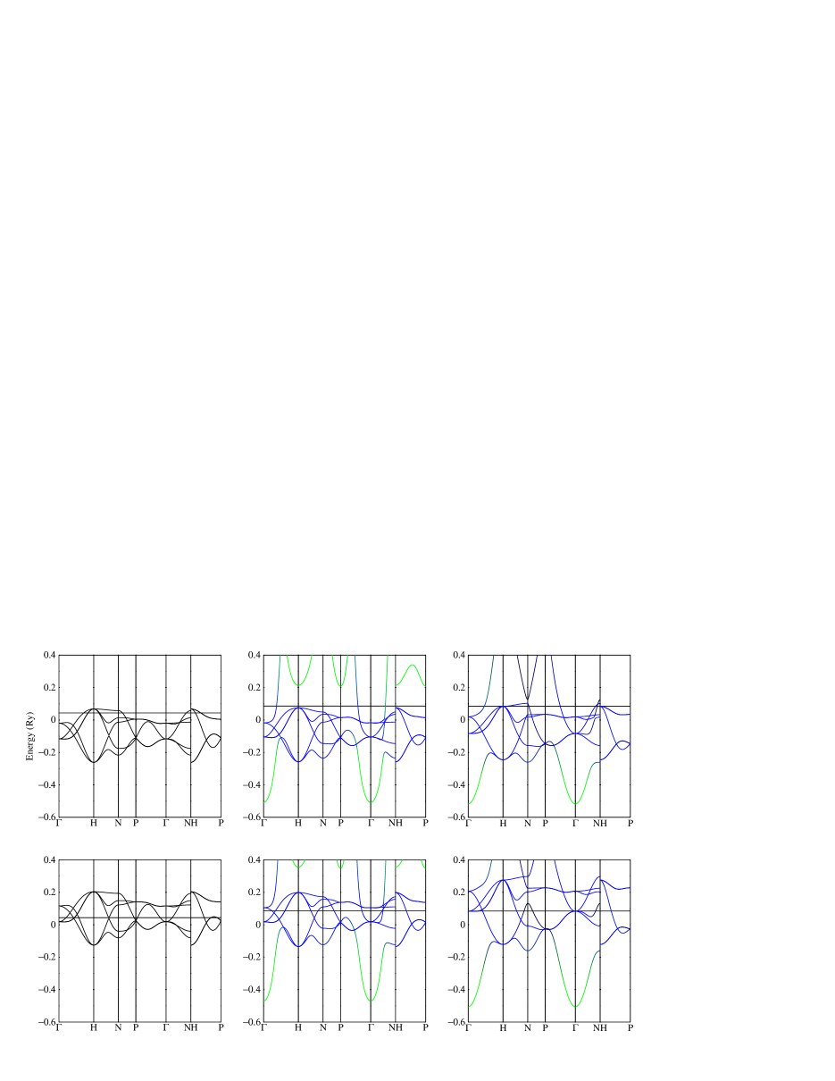
Figure 1: (color online) Energy bands for bcc Fe at its experimental lattice constant, 2.87 Å. The coloring is such that $s$ character is green and $d$ character is blue. The Fermi energy is indicated by a horizontal line. The upper panels are majority and the lower panels minority spin bands. Far left is the tight binding $d$-band model and in the center our non orthogonal $sd$ model. To the right are bands calculated in the LSDA-GGA.

II The tight binding approximation and transferability

II.1 Distance scaling and range of the hopping integrals

There is no need to rehearse the tight binding approximation in any detail here. Recently Paxton and FinnisPaxton and Finnis (2008) constructed tight binding models for magnetic Fe and Fe–Cr alloys and details can be found there as well as in many other publications.Harrison (1980); Pettifor (1995); Finnis (2003); Liu et al. (2005); Pax However we do wish to make some preliminary remarks. The scheme that we use is the self consistent Stoner model for itinerant ferromagnetismLiu et al. (2005) and goes beyond the fixed moment and rigid band approximations. The connection between tight binding theory and the first principles local spin density approximation (LSDA) to density functional theory (DFT) is now well established.Foulkes and Haydock (1989); Sutton et al. (1988); Finnis (2003) TB is computationally several orders of magnitude faster than LSDA because the hamiltonian is constructed from a look-up table of parameterized hopping integrals, $h$, and possibly overlap integrals, $s$. These are conventionally written in Slater and Koster’s notationSlater and Koster (1954) as $ss\sigma$, $sd\sigma$, $dd\sigma$, $dd\pi$, $dd\delta$. Central to a tight binding model is the way in which these integrals scale with bond length. In this work we will useDucastelle (1970); Spanjaard and Desjonquères (1984); Paxton (1996); Paxton and Finnis (2008)

$$h(r)=h_{0}{\rm e}^{-qr}$$ (1)

and similarly for overlap integrals, when used,

$$s(r)=s_{0}{\rm e}^{-qr}.$$ (2)

The alternative is to use the power law scaling, $h\sim r^{-n}$, demanded by canonical band theory.Heine (1967); Andersen (1973, 1975); Pettifor (1977) There is no strong argument to prefer one over the other; in fact by equatingSkinner and Pettifor (1991) logarithmic derivates of $h(r)$ at, say first neighbors at a distance $r_{0}$, we have $n=qr_{0}$ and in the bcc structure of Fe $q\approx 1$ a.u. corresponds to the canonical $n=5$ (see table 1, below).

This brings us to a well known paradox of tight binding modeling namely that the decay of the hopping integrals is known a priori from band theory, which may render them longer ranged than is desirable. A well known example is the group IV semiconductors where by analogy with the free electron bands, to reproduce the volume dependence of the bandwidth the hopping integrals must scale with $n=2$.Froyen and Harrison (1979) This scaling is bound to lead to very long ranged hopping integrals; on the other hand it is known that the first neighbor approximation is the right one, and attempts to include further neighbors fail.Paxton et al. (1987) For many purposes it is adequate simply to cut off the interactions between first and second neighbors, but this can lead to difficulties in work on complex defects or in molecular dynamics. An elegant solution was provided by Goodwin, Skinner, and PettiforGoodwin et al. (1989) (GSP) which cuts off a power law exponentially beyond some chosen cut-off distance, $r_{c}$. There are two drawbacks to this. (i) An exponential decay can still lead to discontinuities in molecular dynamics (as one still needs to impose a cut-off in the neighbor lists). (ii) The GSP form maintains the value but not the slope of the underlying power law at first neighbors. Therefore our preference is to retain the power or exponential scaling given by the canonical band theory and to choose two distances, $r_{1}$ and $r_{c}$, between which to smoothly augment the interaction to zero. This can be achieved by matching value, slope and curvature at $r_{1}$ and at $r_{c}$ with a fifth degree polynomial which replaces the hopping integral in that range.Znam et al. (2003) We show our hopping integrals thus augmented at figure 8 in section IV below, where we discuss this matter further.

II.2 The pair potential, transferability, and non orthogonality

The hopping integrals provide an attractive force, which in the conventional tight binding models is balanced by a repulsive pair potential, which here may take the form

$$\phi(r)=B_{1}{\rm e}^{-p_{1}r}-B_{2}{\rm e}^{-p_{2}r}$$ (3)

in which, as suggested by Liu et al.Liu et al. (2005), both $B_{1}$ and $B_{2}$ are positive. This potential is expected to be repulsive at short range but is not positive for all $r$ (see Fig. 4, below).

An additional non pairwise repulsion is provided if it is chosen to make the model basis non orthogonal. This may give a number of advantages.Paxton and Finnis (2008) One is, that it is widely believed that non orthogonality confers a greater transferability to the model.Allen et al. (1986) By this is meant that a model constructed for a particular crystal structure is less likely to fail when transferred into a situation of different crystal structure or increased or reduced coordination. We will wish to focus critically on this aspect of our models below. It is instructive at this stage to recall that by its very construction the tight binding approximation discards all three center terms in the hamiltonian.Pax On the one hand the canonical band theory shows that these, like non orthogonality, are of second order in the band width.Pettifor (1972, 1977); Andersen and Jepsen (1984) On the other hand Tang et al.Tang et al. (1996) and Haas et al.Haas et al. (1998) took the important step of proposing environment dependent hopping integrals. In this empirical scheme the hopping integral between two atoms is modified in the close proximity of a third atom—in the extreme limit this third atom may approach the two center bond, generally speaking weakening or “screening” it, and eventually come in between the two atoms. Whereas the screening was first described by an empirical formula, Pettifor succeeded in deriving the Tang et al.Tang et al. (1996) expression from the Löwdin transformation of the non orthogonal hamiltonian.Nguyen-Manh et al. (2000) In particular he showed that $sd$ overlap matrix elements in pure transition metals provide this “screening” of the two center bond. Therefore rather than adopting explicit environment dependence as is done in recent bond order potentials,Mrovec et al. (2004, 2007) we retain the two center approximation and employ non orthogonal models to account for the screening.

II.3 The choice of parameters

A related and highly significant findingNguyen-Manh et al. (2000) is that hopping integrals extracted from an LSDA hamiltonian calculated using the tight binding LMTO-ASA methodAndersen and Jepsen (1984) are discontinuous between first and second neighbors in bcc transition metals. These discontinuities are described consequently by the screening—a feature of the geometry of the bcc lattice—leading to the analytic form of Tang et al.Tang et al. (1996) and Haas et al.Haas et al. (1998) The point we wish to raise here is that it became clearNguyen-Manh et al. (2000) that transferable hopping integrals may be extracted from an LSDA hamiltonian thus avoiding the usual need for fitting.Nguyen-Manh et al. (2000); Pax Of course there is no unique tight binding model for a given element since the LSDA hamiltonian is basis-set dependent. We do not adopt this approach here for two reasons. First, the hopping integrals deduced from the LMTO-ASANguyen-Manh et al. (2000); Pax derive from a hamiltonian whose on-site matrix elements are strongly volume dependent whereas in the tight binding approximation these terms are volume independent and hence any volume dependence of the electronic structure must be taken up by the scaling law (1). Second, if the hopping integrals and their scaling are taken from ab initio bandstructures without permitting further adjustment, then essential properties such as elastic constants, lattice constants and structural energy differences may have to rely on the choice of pair potential placing a large burden on that part of the model which is the most ad hoc.

III Models of pure iron

Table 1: Parameters of our tight binding models for pure Fe. The {$h$} and {$s$} are the $h_{0}$ and $s_{0}$ of equations (1) and (2). All quantities are given in atomic Rydberg units (1 bohr = 0.529 Å, 1 Ry = 13.61 eV). Note that in the minimal basis, orthogonal $d$ model, the number of $d$-electrons, $N_{d}$ is a parameter.Liu et al. (2005) Both hopping integrals and pair potentials are smoothly cut off between distances $r_{1}$ and $r_{c}$. These are shown in units of the bcc lattice constant, $a$. Both pair potentials are cut off with $r_{1}=1.1$ and $r_{c}=1.4$, that is, between second and third neighbors of the bcc lattice (see Fig. 4 below). By expressing $r_{1}$ and $r_{c}$ in units of $a$ we imply that these scale with the lattice constant, for example in the calculation of the bulk modulus, so that in a perfect lattice first and second neighbors always see the “proper” pair potential (3) and hopping integrals. This also applies below (Fig. 6) to energy–volume curves in FeH, both for first and second bcc neighbors and first fcc neighbours.

model	orthogonal $d$				non orthogonal $sd$
$\varepsilon_{s}-\varepsilon_{d}$	—				0.15
	$h_{0}$/$s_{0}$	$q$	$r_{1}$	$r_{c}$	$h_{0}$/$s_{0}$	$q$	$r_{1}$	$r_{c}$
$h_{dd\sigma}$	–4.464	1	1.1	1.4	–2.438	0.9	1.1	1.4
$h_{dd\pi}$	2.976	1	1.1	1.4	1.997	0.9	1.1	1.4
$h_{dd\delta}$	–0.744	0.94	1.1	1.4	–0.907	0.9	1.1	1.4
$h_{sd}$	—	—	—	—	–0.141	0.3	1.1	2.0
$h_{ss}$	—	—	—	—	–0.350	0.3	1.1	2.0
$s_{sd}$	—	—	—	—	0.50	0.6	1.1	2.0
$s_{ss}$	—	—	—	—	0.45	0.5	1.1	2.0
$N_{d}$	6.80				—
$I$	0.050				0.055
$B_{1}$	1248.0				536.0
$p_{1}$	1.4510				1.4900
$B_{2}$	1025.0				371.2
$p_{2}$	1.4087				1.4131

III.1 Orthogonal $d$, and non orthogonal $sd$ models

Construction of a tight binding model for transition metals is quite straight forward if it is not required to take the parameters from first principles bandstructure calculations.Paxton and Finnis (2008) Given that the scaling should be close to canonical, as should the ratios,Pettifor (1977)

$$dd\sigma\hskip 6.0pt:\hskip 6.0ptdd\pi\hskip 6.0pt:\hskip 6.0ptdd\delta\hskip 6.0pt\approx-6\hskip 6.0pt:\hskip 6.0pt4\hskip 6.0pt:\hskip 6.0pt-1$$

it is simple enough to guess a set of hamiltonian and overlap matrix elements and adjust these until the resulting energy bands match reasonably closely those from the LSDA. In fact, in all that follows we have used the LSDA with a generalized gradient correction (GGA) of Perdew et al.Perdew et al. (1997) With the exception of data taken from the literature all our LSDA-GGA results are calculated using the full potential LMTO method.Methfessel et al. (2000) Energy bands calculated in this way are shown on the right in Fig. 1. A simple canonical $d$-band model produces the bands shown to the left of Fig. 1. In addition to the integrals already discussed, we require a Stoner parameter, $I$, which represents an on-site Coulomb integral,Pettifor (1995); Paxton and Finnis (2008) to achieve a splitting of the up and down spins.Liu et al. (2005); Paxton and Finnis (2008) Furthermore since the canonical model omits the $s$-band which is occupied by roughly one electronPettifor (1977) it is necessary to fix a number of $d$ electrons, $N_{d}$.Paxton (1996); Liu et al. (2005) This is both the most simple and most reliable model for transition metals.Pettifor (1979); Williams et al. (1980); Pettifor (1987, 1995) Nevertheless for the present purposes we wish to extend this model. In the interests of transferability and to account for the bond screening without explicit environment dependent bond integrals, we explore here the addition of an $s$-orbital to the basis, including $sd\sigma$ and $ss\sigma$ non orthogonality. We will also give arguments for this necessity when we come to the iron hydrides below. The resulting bands, again obtained by simple comparison by eye with the LSDA-GGA bands are shown in Fig. 1. Densities of states associated with the LSDA-GGA and tight binding models are shown in Fig. 2.

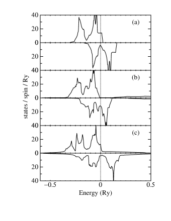
Figure 2: Densities of states of pure bcc Fe in the orthogonal $d$ (a) and non orthogonal $sd$ (b) tight binding models compared to the LSDA-GGA (c). Majority and minority spin states are shown in the upper and lower panels of each. The zero of energy is shifted to the Fermi energy.

Table 2: Calculated properties using parameters from table 1. They are compared in the right hand column to either experimental values or values calculated using LSDA-GGA, the latter written in italics. A proper comparison of the cohesive energy, $E_{{\text{coh}}}$, with experiment should take account of the spin polarization energy of the free atom which is absent in the tight binding limit of infinite separation; this energy is as much asPhilipsen and Baerends (1996) 0.32 Ry so that the calculated $E_{{\text{coh}}}$ should amount to 0.63 Ry. Hence the apparent better agreement of the orthogonal $d$ model is misleading. Both ferromagnetic (FM) and non magnetic (NM) fcc Fe is included; we compare the experimental data to the FM calculations: the lattice constant is extrapolated to 0^∘K;Seki and Nagata (2005) the elastic constants are taken from phonon dispersion curvesZarestky and Stassis (1987) measured at 1428^∘K which is above the Curie temperature (1043^∘K) although local moments are expected to persist.Edwards (1983) LSDA-GGA NM values in parentheses refer to the low spin phase.

		$d$	$sd$
bcc	$a$ (Å)	2.87	2.87	2.87, 2.84
bcc	$K$ (GPa)	175	184	170, 173
bcc	$C^{\prime}$ (GPa)	48	43	52, 62
bcc	$c_{44}$ (GPa)	118	108	121, 109
bcc	moment ($\mu_{B}$)	2.7	2.2	2.2
bcc	$E_{{\text{coh}}}$ (Ry)	0.36	0.51	0.31
hcp	$a$ (Å)	2.54	2.51	2.54
hcp	$K$ (GPa)	164	171	160
hcp	moment ($\mu_{B}$)	2.4	1.8	2.4
hcp	$E_{mag}$ (mRy)	7.7	4.6	7.7
$\Delta E_{{\text{coh}}}$ hcp–bcc (mRy)		12	3	15
fcc (FM)	$a$ (Å)	3.68	3.60	3.55, 3.64
fcc (FM)	$K$ (GPa)	223	187	133, 191
fcc (FM)	$C^{\prime}$ (GPa)	13	12	16, –88
fcc (FM)	$c_{44}$ (GPa)	79	74	77, 13
fcc (NM)	$a$ (Å)	3.45	3.51	3.46 (3.45)
fcc (NM)	$K$ (GPa)	358	232	294 (294)
fcc (NM)	$C^{\prime}$ (GPa)	96	72	102 (102)
fcc (NM)	$c_{44}$ (GPa)	227	151	250 (249)

Having obtained two sets of bond integrals, we proceed to find parameters of the pair potential and we do this by adjusting the four parameters in (3) to the lattice constant and the three elastic constants of bcc Fe. This cannot be done exactly because of the restricted form of the pair potential. The parameter sets are given in table 1 and resulting properties are in good agreement with experiment or LSDA-GGA calculations as can be seen in table 2. Calculations, written in italics in table 2, have been done using the full potential LMTO methodMethfessel et al. (2000) and elastic constants are all obtained at the theoretical lattice constants. Our calculated lattice and elastic constants are in general agreement with previous work.Guo and Wang (2000)

III.2 Predictions of the models

III.2.1 Magnetic moment and structural magnetic energy differences

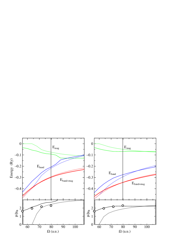
Figure 3: (color online) Contributions to the energy–volume relation in the orthogonal $d$ (left) and non orthogonal $sd$ (right) tight binding models. The lower panel shows the volume dependence of the magnetic moment. The dotted lines refer to the hcp crystal structure and show the rapid collapse of the moment under pressure. The solid line is the bcc moment and may be compared with the circles which are LSDA-GGA calculations. The upper panel shows the bandstructure energy (blue) and the magnetic energy (green) and their sum in red. Solid lines refer to bcc and dotted lines to hcp. The pair potential energy favors bcc in both models. A vertical line indicates the equilibrium volume in bcc Fe.

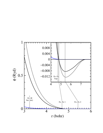
Figure 4: (color online) Pair potentials in the orthogonal $d$ (dotted line) and non orthogonal $sd$ (solid line) tight binding models. Note how these are negative at some of the critical bond lengths. While this helps to stabilize bcc against hcp, the real benefit is in obtaining a correct elastic constant $C^{\prime}$. For reference below we also show here the Fe–H pair potential in blue (see table 5). Vertical lines are placed at first and second neighbor distances in bcc Fe and at first neighbor distances in hcp Fe.

It should be noted that the two models we have described are rather intuitively obtained and so, apart from the pair potential it cannot be said that these are “fitted” in the sense of a classical potential. Hence the properties shown in table 2 are in essence predictions of the model, validating the underlying correctness of the tight binding theory. These predictions can be discussed in more detail by reference to Fig. 3 which shows the structural energy–volume relation in bcc and hcp Fe broken down into bandstructure energy and magnetic energy contributions.Paxton and Finnis (2008) Both models reproduce the essential features which are, (i) the rapid collapse of the hcp magnetic moment under pressure; (ii) the slow decline of the bcc moment and (iii) the stabilization of bcc over hcp being a result of the magnetism. The role of the pair potential warrants explanation here. Fig. 4 shows equation (3) plotted using the parameters of our two models from table 1. It might well be supposed that the stability of the bcc phase compared to the hcp is an artefact of the negative region of $\phi(r)$ falling at the second neighbors of the bcc structure, while the 12 hcp nearest neighbor distances fall in a positive region. This would be a valid criticism of our and Liu et al.’sLiu et al. (2005) models but is misleading. In fact we find that we can easily make models that stabilize bcc employing a pair potential that is positive everywhere. In addition the stabilisation of the bcc structure can be amplified by choosing larger Stoner $I$ parameter. We allow a larger moment in our orthogonal $d$ model since it is known that the magnetic moment in bcc Fe would be closer to $2.6\mu_{B}$ in the absence of $sd$ and $pd$ hybridization.Heine et al. (1980); Hasegawa and Pettifor (1983) Therefore the LSDA-GGA bcc–hcp energy difference is better rendered in that model (table 2) whereas we have chosen a value of $I$ in our non orthogonal $sd$ model that strikes a compromise between a smaller bcc–hcp energy difference having the benefit of a magnetic moment closer to the observed value. The real benefit of the form (3) is that it enables a sufficiently large value of the elastic constant $C^{\prime}$ which otherwise appears too small. It is well known that $C^{\prime}$ can become very soft in bcc metals and the values we obtain in table 2 are the best we can achieve after many trials with the other parameters and scalings in the models. Indeed in the model of Liu et al.Liu et al. (2005), $C^{\prime}$ is significantly lower than ours. The only solution we know of to fit the elastic constants exactly is to employ a spline form for the pair potential as is done in the fitting of bond order potentials,Znam et al. (2003); Mrovec et al. (2004, 2007) and we are rather reluctant to make such a departure from physical intuition.

III.2.2 fcc $\gamma$-Fe

Because our models were fitted to the bcc Fe lattice and elastic constants, it is important to focus on the lower part of table 2 which deals with the fcc phase of Fe. This is $\gamma$-Fe which is the base for the austenitic steels and the crystal structure adopted by pure Fe above 1185^∘K.Leslie (1981) It is well knownKaufman et al. (1963); Roy and Pettifor (1977); Christensen et al. (1988); Elsässer et al. (1998) that $\gamma$-Fe exists in a high spin ferromagnetic and a low spin (approximately non magnetic) modification and we show predictions for both phases in table 2 which we compare with LSDA-GGA calculations and experimental observations. It is a mark of transferability that both models give a good account of each of the two fcc phases. Neither model fully captures the large and negative $C^{\prime}$ or the softening of $c_{44}$ of the LSDA-GGA in the high spin phase; although they are in better accord with experiment than the LSDA-GGA, the proper comparison is with the 0^∘K calculations. The elastic softening in $\gamma$-Fe is consistent with the measured temperature dependence of $C^{\prime}$ in the Invar alloys,Tajima et al. (1976) therefore it is encouraging that our models are able to describe this important physical phenomenon at least in principle. It has already been shown that elastic and phonon softening with increasing temperature in $\alpha$-Fe is captured in the tight binding approximation.Hasegawa et al. (1985, 1987)

Table 3: Calculated surface energies in J/m². Values in parentheses are for truncated bulk (unrelaxed) surfaces. LSDA-GGA calculations are taken from Spencer et al.Spencer et al. (2002)

model	orthogonal $d$	non orthogonal $sd$	GGA
(110)	1.77 (1.77)	1.53 (1.56)	2.27 (2.27)
(001)	2.12 (2.15)	1.74 (1.79)	2.29 (2.32)
(111)	3.54 (3.85)	2.80 (3.34)	2.52 (2.62)

III.2.3 Surface energies

The proper test of transferability is to carry the models into situations of over or under coordination. Here, we do this by addressing the surface energies of pure Fe. We have set up the (110), (001) and (111) surfaces of bcc Fe and relaxed the atom positions by energy minimization using the Hellmann–Feynman forces.Finnis et al. (1998); Liu et al. (2005); Pax The resulting energies are shown in table 3 in order of decreasing coordination, the most close packed surface being (110). We achieve modest, but satisfactory agreement with published LSDA-GGA calculationsSpencer et al. (2002) at least for the two most close packed surfaces. It is in fact notable that the LSDA-GGA predicts all the surfaces to have nearly the same energy with (111) being a little higher. This is not reflected in the tight binding models, indicating limits to their transferability. The orthogonal $d$ model gives the greater spread in energies, demonstrating to some extent the greater transferability afforded by the inclusion of an $s$ orbital. It is gratifying that both models give a qualitative account of surface energies without having been fitted, at least in the case of the (110) and (001) the latter being of most importance as it’s the usual cleavage face.Allen et al. (1956); Leslie (1981); Ayer et al. (2006) It is also significant in the present context that the effect of H on pure Fe and Fe–Si is to enable cleavage also on the (110) planes.Nakasato and Bernstein (1978)

III.2.4 Vacancy formation energy

Table 4: Vacancy formation energy, $E_{v}^{f}$, in eV, of pure Fe, calculated with the orthogonal $d$ and non orthogonal $sd$ tight binding models and compared to published LSDA-GGA and experimental results.

model	$d$	$sd$	LSDA-GGA	expt.
relaxed	2.39	1.33	1.95, 2.18	1.61–1.75, 1.59
			2.09	$2.0\pm 0.2$
unrelaxed	2.42	1.36	2.24, 2.60

A further test of the transferability is to predict the formation energy of a vacancy. We do this by constructing 54 and 53 atom “supercells” of bcc Fe ($3\times 3\times 3$ cubic two-atom unit cells), one of which has an atom missing. The structure is relaxed by energy minimization; its resulting total energy is denoted $E(\text{Fe}_{53})$. The energy of the 54 atom supercell is denoted $E(\text{Fe}_{54})$. Then the vacancy formation energy, neglecting volume relaxation, isGillan (1989)

$$E_{v}^{f}=E(\text{Fe}_{53})-\frac{53}{54}\>E(\text{Fe}_{54}).$$

Our results are shown in table 4 which also gives values for the “unrelaxed” vacancy. As for the surface energies, $E_{v}^{f}$ is underestimated by the non orthogonal $sd$ model and overestimated by the orthogonal $d$ model. The likely error compared to experiment in the latter however is more than twice that of the non orthogonal $sd$ model, again demonstrating some benefit in transferability of including the non orthogonal $s$-orbitals.

IV Adding Fe–H interactions

Figure 5: (color online) To illustrate the tetrahedral (T) and octahedral (O) interstices in the bcc (upper figure) and fcc (lower figure) crystals. Note that in the bcc lattice the octahedral site is at the center of a distorted octahedron, unlike the fcc where it is regular. The distance to the two apical atoms, shown here as a horizontal bond, is shorter by a factor $1/\sqrt{2}$ than the distances to the equatorial atoms, two of which are shown here in the upper face. This leads in general to the well known tetragonal distortion of the bcc lattice near octahedral interstitial atoms, for example in martensite. For details see refs [Barrett and Massalski, 1966; Leslie, 1981]. Neither is the tetrahedral interstitial site in the bcc lattice regular—indeed both octahedral and tetrahedral bcc interstices have tetragonal symmetry. The fcc crystal structure with all the octahedral sites occupied becomes that of cubic rocksalt adopted by many transition metal carbides and nitrides. In fcc, the tetrahedral site is regular; when half these sites are occupied the resulting crystal structure is that of zincblende.

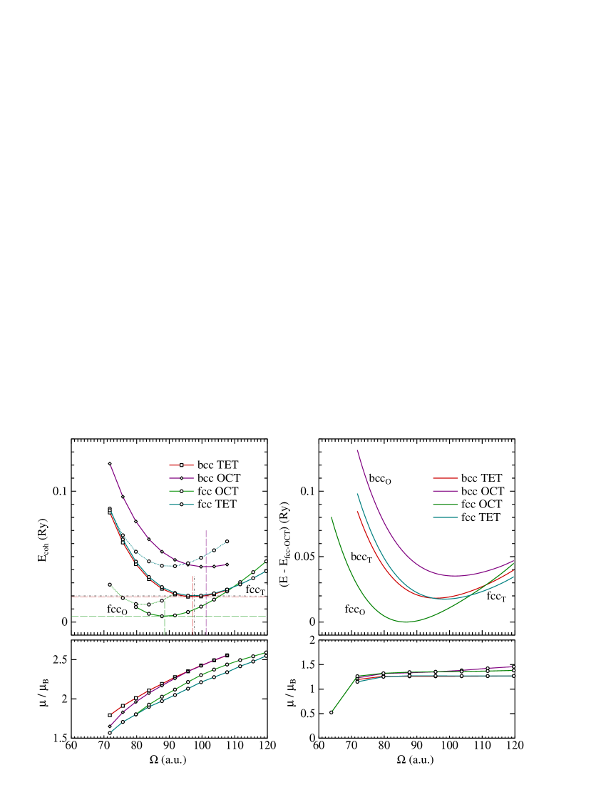
Figure 6: (color online) Cohesive energy and magnetic moment as a function of volume per Fe atom in the four FeH phases calculated within the LSDA-GGA (left). Dotted lines denote non magnetic phases. The cohesive energy is with respect to solid $\alpha$-Fe and molecular H₂ also calculated using the same energy functional and hence is an approximation to the heat of formation. Note that on this basis none of the phases is expected to exist. On the right we show the same quantities calculated in the non orthogonal $sd$ tight binding model. We expect that the almost exact degeneracy of bcc TET and fcc TET is accidental.

As emphasized before, we will keep the parameters of pure Fe unchanged as we seek a model for H in Fe. We will find such a model by comparison with properties of iron monohydrides of stoichiometry FeH, that is, the concentrated limit and then test our model’s transferability into the dilute limit.

In a series of three papers,Elsässer et al. (1998, 1998, 1998) Elsässer et al. have made a comprehensive study of the compound FeH in the framework of density functional theory. One is interested in four putative phases, namely fcc and bcc Fe each having one H atom in either tetrahedral or octahedral sites. These are illustrated in Fig. 5; and Fig. 6 shows energy–volume curves for these four phases calculated using LSDA-GGA in the full potential LMTO methodMethfessel et al. (2000) (see also Fig. 5 in ref [Elsässer et al., 1998]).

Figure 7: (color online) Energy bands for bcc tetrahedral FeH, calculated at the lattice constant of pure bcc Fe. The upper panels show majority and the lower minority spin states. The coloring is such that H-$s$ character is red and Fe-$d$ character is blue. Fe-$s$ bands are green. The Fermi energy is indicated by a horizontal line. Note that the Fe-$4s$ band has been pushed above the $d$-bands. Bands on the left are from our tight binding model and on the right are bands calculated in the LSDA-GGA.

Examination of the upper sketch in Fig. 5 shows that the displacement of the tetrahedral interstitial atom in the bcc structure towards the octahedral site brings the impurity atom from above the second neighbor bond, at right angles until it finally rests at the bond center. This is precisely the situation envisaged by Haas et al.Haas et al. (1998) in their proposal of the screening function, and we therefore expect for a model to be transferable, we will require it to be non orthogonal. There is also a strong argument for the retention of the Fe $4s$ orbital even though, as we have seen, it does not lead to a significantly better model for pure Fe than the orthogonal $d$.Paxton (1996) The argument for its inclusion follows from an examination of Fig. 7 which shows LSDA-GGA energy bands for bcc tetrahedral FeH. The bands are colored according to the eigenvector weights coming from LMTO’s from H $1s$ (red) or Fe $3d$ (blue). The H $1s$ band is split off from the Fe $3d$ bands and has similar width. The Fe $4s$ band which in pure Fe has its bottom below the Fe $3d$ bands and which hybridizes with them (see Fig. 1) is pushed up above the top of the Fe $3d$ bands by repulsion of the H $1s$ band. This means that the Fermi energy remains near where it is in pure Fe. Roughly speaking one might say that the single $4s$ electron per atom in pure Fe is transferred to the hydrogen atom to complete its 1$s$ shell, or rather to fill the H $1s$ band. At first glance it may seem natural to neglect the Fe $4s$ bands in FeH. But a difficulty will arise if we adapt a $d$-only model by adding just an extra H $1s$ orbital. Hydrogen brings one electron with it and to fill the split-off H $1s$ band an electron will be drawn down from the Fe $3d$ bands consequently lowering the Fermi level. If we were only interested in FeH then we could just adjust $N_{d}$, the number of $d$ electrons; but this will introduce an inconsistency in going to the dilute limit: $N_{d}$ will somehow need to be continuously adjusted at Fe atoms successively further away from an impurity H. It is very hard to see how this problem could be overcome except possibly by alloting two electrons to the hydrogen impurity; while it is solved naturally by the Fe $4s$ falling back into place as an Fe atom finds itself remote from the influence of impurity. We emphasize that in the non orthogonal $sd$ model and its extension to impurities the number of electrons is not a parameter—as long as all occupied bands are included in the hamiltonian we can happily take the number of electrons from the periodic table.

Therefore we take over the pure Fe non orthogonal $sd$ model and we add parameters to account for the additional H $s$ band. We need Fe–H $sd\sigma$ and $ss\sigma$ hopping and overlap parameters but we do not require H–H interaction parameters since even the closest approaching interstitial sites are distant more than three times the length of the H₂ molecular bond. The $sd\sigma$ and $ss\sigma$ integrals establish the width of the H $s$ band while its position with respect to the $d$ bands is set by the on-site energy, $\varepsilon_{s}$ of the H $s$ orbital. We also require Hubbard-$U$ parametersFinnis et al. (1998); Finnis (2003) for H and Fe, but these are not critical and 1.2 Ry and 1 Ry are good choices. Essentially these lead to approximate charge neutrality as expected in metals and their alloys.Pettifor (1987) For simplicity we take the Stoner parameter for H to be zero. Tetrahedral bcc FeH is ferrimagnetic, both in LSDA and in our tight binding model, the H atom carrying a small moment, less than 1 $\mu_{\text{B}}$ (aligned opposite to that of the Fe atom cf., Fig. 8 in ref [Elsässer et al., 1998]).

Table 5: H on-site, and Fe–H interaction parameters of our tight binding model. All quantities are given in atomic Rydberg units. For all these integrals we use $r_{1}=0.8$ and $r_{c}=2$ in units of the pure Fe bcc lattice constant, $a=2.87$ Å; for the pair potential we use $r_{1}=0.8$ and $r_{c}=0.95$ in the same units.

$\varepsilon_{s}-\varepsilon_{d}$	–0.085
$U_{\hbox{Fe}}$	1.0
$U_{\hbox{H}}$	1.2
		$q$
$h_{ss}$	–0.35	0.776
$h_{sd}$	–0.14	0.454
$s_{ss}$	0.27	0.286
$s_{sd}$	0.22	0.473
$B$	299.6
$p$	2.6922

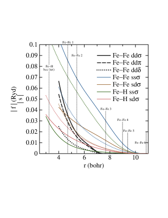
Figure 8: (color online) Hopping and overlap integrals as functions of bond length, $r$, in the $sd$ non orthogonal model. Except in the case of $dd\delta$ the dotted lines are the overlap integrals corresponding to the hopping integrals of the same color. Vertical dotted lines indicate the Fe–H bond length in bcc tetrahedral FeH at equilibrium volume, and the Fe–Fe bond lengths of the first six neighbors in pure bcc Fe.

To find the additional parameters we have resorted to fitting these to the four equilibrium atomic volumes and three cohesive energy differences marked with dashed lines on Fig. 6. We do this using Schwefel’s multimembered evolution strategy.Schwefel (1977, 1993) For the Fe–H pair potential we employ

$$\phi(r)=\frac{B}{r}\>{\rm e}^{-pr}.$$

The resulting parameters are displayed in table 5 and the hopping integrals are shown graphically in Fig. 8 to illustrate their relative magnitudes and ranges. In the same figure we show the hopping integrals for Fe which are, of course, identical to those of our non orthogonal $sd$ model of section III. With reference to our remarks in section II.1 we note that all our hopping and overlap integrals have the simple exponential form up to the distance $r_{1}$ beyond which they are augmented so as to go continuously and differentiably to zero at $r_{c}$. These distances are not strictly parameters of the model and are not used in the fitting. They are chosen intuitively; for example one expects just first neighbors in hcp and fcc, and first plus second neighbors in the bcc structures to be interacting through $dd$ hopping whereas the $s$ electrons in pure Fe are essentially free electron like and hence “do not take kindly to being treated within a TB framework”.Pettifor (1977) They are best represented by longer ranged interactions. These points are illustrated in Fig. 8 and the values of $r_{1}$ and $r_{c}$ can be found in tables 1 and 5. The use of fifth degree polynomials to augment the tails is necessary to acheive a smooth join; it can lead to small kinks as seen in Fig. 8, but these are designed to fall in between neighbor shells and so minimize their effect. This is why the parameters $r_{0}$ and $r_{c}$ are made to scale with the lattice constant. The resulting energy bands are plotted in Fig. 7 for comparison with the LSDA-GGA bands. The resulting energy volume curves are shown in Fig. 6. The TB model does not reproduce the magnetic moments of the LSDA-GGA in Fig. 6 quantitatively since this is a sensitive function of the density of states at the Fermi level in the non magnetic crystal and our energy bands are only in qualitative agreement with the LSDA-GGA.

Table 6 summarizes the equilibrium properties of the four hydride phases shown in Fig. 6. The question of site selectivity, especially in bcc Fe is important and we will revisit it in the dilute limit, below, in section V.2.1.

Table 6: Equilibrium volumes per Fe atom and cohesive energies of the four FeH phases following evolution optimisation, compared to the target values. Cohesive energies are relative to the fcc octahedral (rocksalt) phase. The final column shows the radius of the interstitial site based on a lattice of hard spheres at the equilibrium volume of pure Fe and taken from Leslie.Leslie (1981) All quantities are given in atomic Rydberg units.

	TB		Target		radius
	$E_{\hbox{coh}}$	$\Omega$	$E_{\hbox{coh}}$	$\Omega$
fcc OCT	0.0	86.90	0.0	88.59	0.98
fcc TET	0.017	98.64	0.016	97.58	0.53
bcc TET	0.018	96.16	0.015	97.23	0.68
bcc OCT	0.035	101.75	0.038	101.28	0.36

V Predictions of the Fe–H model

V.1 Iron hydride

Figure 9: (color online) Illustrates the translations of the bcc intersitials in constructing our adiabatic potential surfaces, after the three dimensional drawing of Fig. 1 in Krimmel et al.Krimmel et al. (1994) The figure represents an (010) face of the bcc lattice with Fe atoms as black circles at each corner. The octahedral sites are shown as squares, the central, filled one being the one occupied in octahedral FeH. Of the four tetrahedral sites, shown as triangles, one is occupied in tetrahedral FeH and this is shown filled in here. The point, S, is midway between two tetrahedral sites—the expected diffusion path of H in FeHirth (1980) which is highlighted in red here and in Fig. 10. Those displacements which are in the (010) plane are indicated.

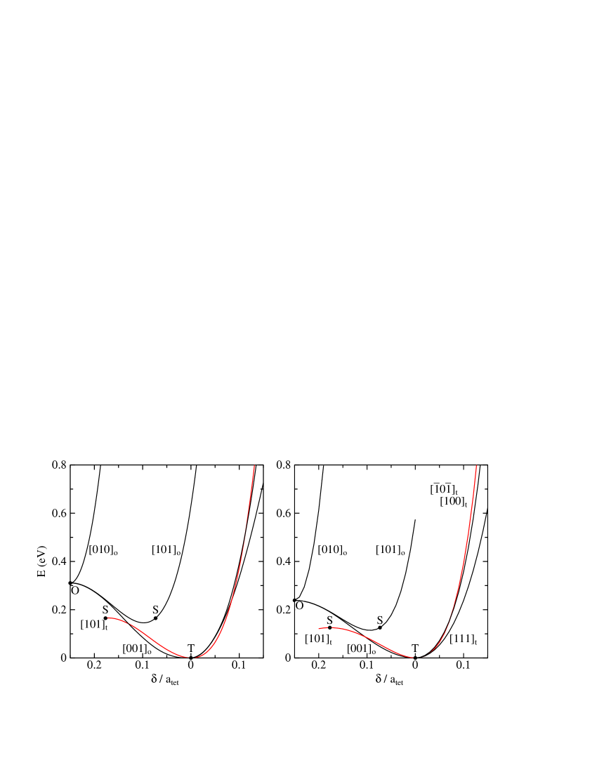
Figure 10: (color online) Adiabatic potential surface sections of bcc FeH: left LDA,Elsässer et al. (1998) right TB. These curves show the energy as a function of the displacement of the H sublattice relative to the Fe sublattice. The curves which start at the point “O” refer to displacements from the octahedral site phase; a H atom initially at position $[\frac{\scriptstyle 1}{\scriptstyle 2}0\frac{\scriptstyle 1}{\scriptstyle 2}]$ translates in the directions indicated. Along the $[001]$ direction it eventually falls into a vacant tetrahedral site (see Fig. 9). This curve hence represents the transition to the tetrahedral-site phase. Translation along $[101]$ takes the H atom to a position midway between two, vacant, tetrahedral sites—this point is marked “S”. For a H atom initially occupying a tetrahedral site, translation along $[101]$ moves it to an adjacent, unoccupied, tetrahedral site, the half-way point being the same point “S”. The translation labels are vectors referred to Fig. 9. For each case, LDA and TB, the calculations are at fixed atomic volume, namely the equilibrium volume of the bcc tetrahedral phase of FeH, see table 6; $a_{0}$ is the corresponding equilibrium lattice constant.

Our first test of the tight binding model is to compare the resulting adiabatic potential surface section with the results of calculations by Elsässer et al.Elsässer et al. (1998); Krimmel et al. (1994) which were made in the local density approximation (LDA) to DFT. In these calculations the H sublattice is displaced with respect to the Fe sublattice in both bcc and fcc FeH in a chosen set of directions so as to explore the curvatures and barriers of the potential energy landscape. For the case of the bcc structure, Fig. 9 shows some of the displacment paths. The potential sections from previous LDAElsässer et al. (1998) and our present tight binding model are shown in Fig. 10. Whereas the relative energies of the tetrahedral and octahedral sites have been established by the fitting, the remainder of the these curves amount to predictions of the tight binding model. They turn out to be be in remarkable, quantitative agreement with the LDA calculations in the bcc and fcc case, the latter being shown in Fig. 11. These curves exploit to the full the notion discussed in section II.2, above, of environment dependent screening of hopping integrals as the hydrogen approaches Fe–Fe first and second neighbor bonds and indeed penetrates the bond to lie directly in between the two atoms. It is exactly in this situation that one expects the Fe–Fe bond integrals to be strongly modified by screening, and clearly our model captures this well in a non orthogonal two center description. In particular note, in reference to Fig. 10 that the minimum energy (saddle) point along the $[101]_{o}$ path lies to the left of the point “S” in both LDA and in our TB model. This implies that the $[101]_{t}$ minimum energy diffusion path in reality is bowed slightly towards the center of Fig. 9. The strongest test of the environment dependence however is in the fcc hydrides of Fig. 11. The energy barrier at the maximum of the $\langle 110\rangle_{o}$ path, coinciding with the maximum of the $\langle 001\rangle_{t}$ path is perfectly rendered by the TB model without having been fitted and this corresponds to the extreme instance of screening in which the H atom becomes positioned at the center of the first neighbor Fe–Fe bond (see Fig. 1, ref [Krimmel et al., 1994]).

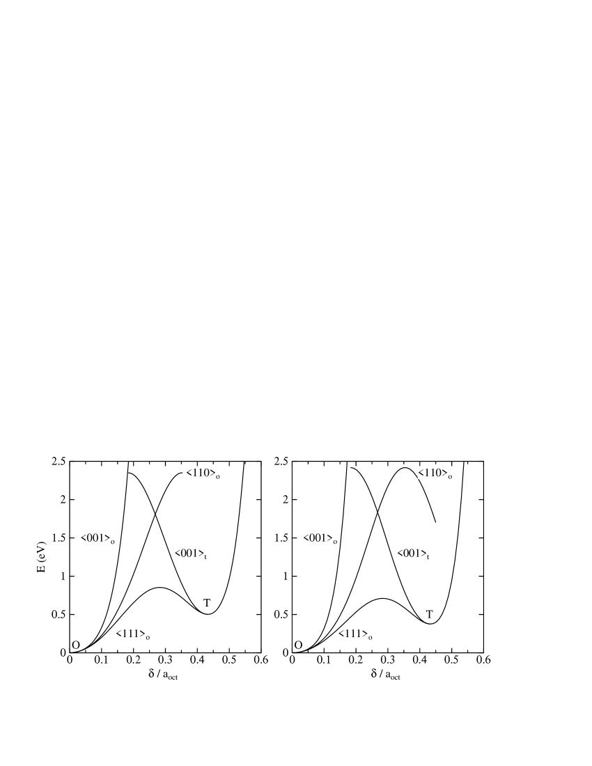
Figure 11: Adiabatic potential surface sections of fcc FeH: left LDA,Elsässer et al. (1998) right TB. At the point “O” we have the rocksalt phase, from which translation of the H sublattice along a $\langle 111\rangle$ direction transforms the structure to the zincblende phase in which tetrahedral sites are occupied. The energy maximum between “O” and “T” is located close to where the H atom squeezes between an equilateral triangle of Fe atoms in the (111) plane. At the maximum along $\langle 110\rangle_{o}$, and along $\langle 001\rangle_{t}$, the H is positioned mid-way between two nearest neighbor Fe atoms (see Fig. 1 of ref [Krimmel et al., 1994]). Note that both these two energy barriers are predicted by the TB model with quantitative accuracy. The calculations are at the calculated equilibrium volume of the fcc octahedral (rocksalt) phase of FeH, see table 6; $a_{0}$ is the corresponding equilibrium lattice constant.

V.2 H in Fe—the dilute limit

We concentrate on three predicted properties of iron in this section. First is the dissolution energyJiang and Carter (2004) or zero temperature heat of solution of hydrogen in Fe. Included in this study is the matter of the site selectivity. Second is the binding energyRamasubramaniam et al. (2009) or 0^∘K segregation energy of H to the (001) surface of Fe. Third, and of great importance to the question of hydrogen embrittlement, is the binding of H atoms to a vacancy in Fe.

V.2.1 Dissolution energy

Following Ramasubramaniam et al.Ramasubramaniam et al. (2009) we construct a 54 atom supercell as we did in section III.2.4 and whose total energy we denoted $E(\text{Fe}_{54})$. We then place a hydrogen atom at either a tetrahedral or an octahedral site and minimize the total energy by relaxation. The resulting total energies are denoted $E(\text{Fe}_{54}H)$. We do not allow the volume to relax. Then the dissolution energy isJiang and Carter (2004)

$$E_{\text{dis}}=E(\text{Fe}_{54}\text{H})-E(\text{Fe}_{54})-\genfrac{}{}{}{1}{1}{2}E_{{\text{H}}_{2}}$$ (4)

Our model does not contain H–H interactions, but faux de mieux we may take $E_{{\text{H}}_{2}}=-4.75$ eV from experiment or from quantum chemistry.Skinner and Pettifor (1991); Jiang and Carter (2004) For each of the three calculations we employ a mesh of $12\times 12\times 12$ ${\bf k}$-points and use first order generalized Gaussian integration of the Brillouin zone with a width of 2.5 mRy.Methfessel and Paxton (1989) Results are shown in table 7. These are in remarkably good quantitative agreement with both observations and LSDA-GGA calculations. In particular we predict the tetrahedral site to be preferred over the octahedral, as is well established.Hirth (1980) We may point out here that this is not a trivial result: carbon in contrast, while preferring the tetrahedral site in the ficticious bcc-based carbide, transfers to the octahedral site in the dilute limit.Paxton (2010) In the effective medium theory, upon which the embedded atom potentials (EAM) are based, H prefers the octahedral site.Puska and Nieminen (1984)

Table 7: Dissolution energy, in eV, of H in Fe in both tetrahedral (TET) and octahedral (OCT) interstices. Present results are marked TB, experimental and LSDA-GGA values are taken from Jiang and Carter.Jiang and Carter (2004)

	TET	OCT
TB	0.273	0.354
expt.	0.296
GGA	0.19	0.32

V.2.2 H segregation to the (001) surface of Fe

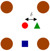
Figure 12: (color online) Three possible binding sites of H on the (001) surface of Fe, after Ramasubramaniam et al.Ramasubramaniam et al. (2009) Four large circles represent the Fe atoms at the corners of a unit cell of the (001) face of the bcc lattice. At the center is the “hollow” site, a smaller circle; this may be displaced along [100] by an amount $\delta$ to become the “quasi-threefold” (QT) site indicated by a triangle. The “bridge” site is shown as a square. It is important to recognize that the bridge and hollow sites in the plane of the truncated bulk surface are octahedral interstices, whereas the QT site at $\delta=0.25a_{0}$ is a tetrahedral site. If a H atom at the bridge site is displaced up or down by $0.25a_{0}$ then it comes to occupy a tetrahedral site. Here, $a_{0}=2.87$ Å is the equilibrium pure $\alpha$-Fe lattice constant.

Three binding sites of H to the (001) surface of Fe have been identified.Ramasubramaniam et al. (2009) These are illustrated in Fig. 12. We have constructed supercells of $2\times 2\times 5$ cubic two-atom unit cells with three layers of vacuum inserted along the long axis. The slab contains 40 Fe atoms and the total energy of the fully relaxed supercell is denoted $E^{\text{surf}}(\text{Fe}_{40})$. We place one H atom at one of the three adsorption sites in Fig. 12 and relax the structure by energy minimization. Allowing all atoms to relax we denote the total energy $E^{\text{surf}}(\text{Fe}_{40}H)$. The associated “adsorption energy” isRamasubramaniam et al. (2009)

$$E_{\text{ads}}=E(\text{Fe}_{54}\text{H})-E(\text{Fe}_{54})-\genfrac{}{}{}{1}{1}{2}E_{{\text{H}}_{2}}$$

and by combining the previous two equations the “binding energy” isRamasubramaniam et al. (2009)

$$E_{\text{bind}}=E_{\text{dis}}^{t}-E_{\text{ads}}$$ (5)

in which the reference energy, or chemical potential, of gaseous H₂ has canceled. $E_{\text{dis}}^{t}$ is the dissolution energy (4) at a tetrahedral site (table 7). We have calculated the three quantities using a $12\times 12\times 1$ ${\bf k}$-point mesh and the same Brillouin zone integration as above. In table 8 we show our calculated binding energies, the displacement $\delta$ in Fig. 12 and the height, $h$, from the (001) surface constructed as the difference in $z$-coordinates of the H atom and the average from the four topmost Fe atoms.

Table 8: Predicted structure and energetics of H adsorbed on Fe (001). We show for the QT, hollow (H) and bridge (B) sites of Fig. 12 the displacent $\delta$ and height, $h$, above the surface (all in Å) and the 0^∘K segregation or binding energy, $E_{\text{bind}}$, in eV. In parentheses are the LSDA-GGA results of Ramasubramaniam et al.Ramasubramaniam et al. (2009)

	$\delta$		$h$		$E_{\text{bind}}$
	TB	(GGA)	TB	(GGA)	TB	(GGA)
QT	0.635	(0.19)	0.31	(0.38)	0.241	(0.768)
H			0.27	(0.38)	0.191	(0.775)
B			0.85	(1.20)	0.222	(0.655)

The predictions of our model are only in reasonable agreement with the LSDA-GGA.Ramasubramaniam et al. (2009) The heights above the surface are well rendered; the displacement, $\delta$, is significantly larger, but is consistent with the preference for tetrahedral site occupancy. As we point out in the caption to Fig. 12, $\delta=0.25a_{0}=0.71$ Å puts the H atom into a surface tetrahedral site and our model does exactly that; in contrast the LSDA-GGA quite surprisingly results in a much smaller $\delta$. In the same vein, the height of the H atom above the bridge site, 0.85 Å, is close to $0.25a_{0}$, and we find another local minimum at 0.34 Å below the bridge site. Thus the strongest binding in the TB model is to surface tetrahedral sites and the surface octahedral site is indeed not a local energy minimum. In this way the binding energies are in poor agreement with the LSDA-GGA and may reflect the limitations in transferability (section II.2) in that the model retains its bulk-like features at the surface. $E_{\text{bind}}$ is in fact the 0^∘K segregation energy, usually defined as the energy needed to remove the impurity from the surface and place it into the interior of the crystal. The LSDA-GGA shows the smallest adsorption energy (largest $E_{\text{bind}}$) to be at the hollow site; whereas we find it at the QT site and at this coverage this is not consistent with experiment which shows a transition at 100^∘K from hollow to QT site selectivity between about 0.3ML and 1ML,Merrill and Madix (1996) while our calculations and the LSDA-GGARamasubramaniam et al. (2009) are at 0.25ML.

Both the QT and bridge sites are at local minima in the potential energy in our model. This is consistent with the LSDA-GGA.Ramasubramaniam et al. (2009) However the hollow site is a local saddle point having an almost flat energy surface with respect to small displacements parallel to the surface; if we displace the H atom a sufficient amount then the structure relaxes into the QT site occupancy. This is inconsistent with the LSDA-GGA in which surprisingly, in view of there being another local minimum at QT just 0.19Å distant, the hollow site is at a local minimum.Ramasubramaniam et al. (2009)

To some extent our choice of chemical potential for $H_{2}$, $E_{{\text{H}}_{2}}$, is arbitrary; however the observed bond energy leads to a very good rendering of the 0^∘K heat of solution (dissolution energy) of H in Fe, table 7. On the other hand it leads to a positive, but small, adsorption energy, $E_{\text{ads}}$, which means that in our model $H_{2}$ will not dissociate on the (001) surface of Fe. In order to model the surface adsorption properly we could make an ad hoc adjustment of $E_{{\text{H}}_{2}}$. This would be at the expense of less accurate $E_{\text{dis}}$. For example, if we used the Skinner and Pettifor tight binding model of hydrogen,Skinner and Pettifor (1991) then we’d have $E_{{\text{H}}_{2}}=-4.30$ eV rather than $-4.75$ eV. In that case our dissolution energy in the tetrahedral site becomes 0.05 eV (rather than 0.27 eV, cf table 7) but the adsorption energies are then negative as they should be. Of course the segregation energies (table 8) remain unchanged by this redefinition of the hydrogen chemical potential.

V.2.3 H segregation to a vacancy in Fe

It is believed that the trapping of H to vacancies in Fe is of central importance in the effects of H on mechanical behavior.Hirth (1980); Takai et al. (2008); Kirchheim (2010) It is also known that dissolved hydrogen results in a dramatic increase in the vacancy concentration in several metals including Fe,Iwamoto and Fukai (1999); Fukai et al. (2003) caused through segregation induced lowering of the vacancy formation enthalpy.Kirchheim (2007) We can show that our model is able to demonstrate these facts by comparison with LSDA-GGA calculations of the 0^∘K segregation energy, $E^{v}_{\text{bind}}(n)$, of up to seven H atoms to a single vacancy in Fe.Ramasubramaniam et al. (2009); Tateyama and Ohno (2003) The principal result, which we also predict in our TB model is that up to five H atoms may bind to a vacancy with a positive segregation energy, but the sixth has a small negative $E^{v}_{\text{bind}}(n)$. Here we follow Tateyama and OhnoTateyama and Ohno (2003) and Ramasubramaniam et al.Ramasubramaniam et al. (2009) and define $E^{v}_{\text{bind}}(n)$ as the 0^∘K segregation energy of a H atom from a bulk tetrahedral site to a vacancy to which $(n-1)$ H atoms are already segregated. Hence we set up a 53 atom supercell as in section III.2.4; then in reference to figure 5 in Ramasubramaniam et al.,Ramasubramaniam et al. (2009) if the vacant site is at $[\genfrac{}{}{}{1}{1}{2}\genfrac{}{}{}{1}{1}{2}\genfrac{}{}{}{1}{1}{2}]$ in the bcc supercell we add H atoms successively in (1) $[\genfrac{}{}{}{1}{1}{2}\genfrac{}{}{}{1}{1}{2}0]$, (2) $[\genfrac{}{}{}{1}{1}{2}\genfrac{}{}{}{1}{1}{2}1]$, (3) $[\genfrac{}{}{}{1}{1}{2}1\genfrac{}{}{}{1}{1}{2}]$, (4) $[\genfrac{}{}{}{1}{1}{2}0\genfrac{}{}{}{1}{1}{2}]$, (5) $[1\genfrac{}{}{}{1}{1}{2}\genfrac{}{}{}{1}{1}{2}]$, and (6) $[0\genfrac{}{}{}{1}{1}{2}\genfrac{}{}{}{1}{1}{2}]$ octahedral interstices—these are the centers of the six {001} faces bounding the vacant site. Finally a seventh H atom may be placed at the vacant site. These supercells are relaxed by energy minimization and we denote the total energy of the supercell by $E({\text{Fe}}_{53}{\text{H}}_{n})$. Then we haveTateyama and Ohno (2003); Ramasubramaniam et al. (2009); Foo in analogy with (5)

$$E^{v}_{\text{bind}}(n)=E_{\text{dis}}^{t}-\left(E({\text{Fe}}_{53}{\text{H}}_{n})-E({\text{Fe}}_{53}{\text{H}}_{n-1})-\genfrac{}{}{}{1}{1}{2}E_{{\text{H}}_{2}}\right)$$

which is independent of the chemical potential of H. Table 9 shows our segregation energies, compared to LSDA-GGA. The relaxation pattern is very simple in all cases except $n=3$ and $n=5$. In the simple instances, each H atom relaxes perpendicularly to its {001} face, by an amount we denote $\delta^{\text{even}}_{\perp}(n)$, towards the vacant site. The displacement decreases as $n$ increases both in LSDA-GGATateyama and Ohno (2003) and our TB model. In each of the cases $n=3$ and $n=5$ there is one H atom which follows this trend whereas the remaining $(n-1)$ H atoms are displaced both towards the vacancy by $\delta^{\text{odd}}_{\perp}(n)$ and, by an amount $\delta_{\parallel}(n)$ in a direction parallel to the {001} face containing the site where the H atom was originally placed, in a $\langle 100\rangle$ direction.

Table 9: Segregation of H atoms to a vacancy in Fe. We show our model’s predicted $E^{v}_{\text{bind}}(n)$ compared to LSDA–GGA results,Tateyama and Ohno (2003) quoted by Ramasubramaniam et al.,Ramasubramaniam et al. (2009) in eV. Also shown are the displacements of the H atom towards the vacancy, and away from the octahedral site in the {001} plane in which it was originally placed. In cases of higher symmetry the displacement of all H atoms is an amount $\delta^{\text{even}}_{\perp}(n)$ normal to the {001} face and towards the vacant site. In the cases $n=3$ and $n=5$ one atom follows this displacement, while all those remaining move both perpendicular to the face—by an amount $\delta^{\text{odd}}_{\perp}(n)$—and parallel to the face in a $\langle 100\rangle$ direction by an amount $\delta_{\parallel}(n)$, rather like the knight’s move in chess. A displacement $\delta_{\parallel}=0.25a_{0}=0.71$ Å will take the H atom into a tetrahedral site. Displacements are given in Å.

$n$	$E^{v}_{\text{bind}}(n)$		$\delta^{\text{even}}_{\perp}(n)$	expt.	$\delta^{\text{odd}}_{\perp}(n)$	$\delta_{\parallel}(n)$
	TB	LSDA-GGA
1	0.319	0.559	0.25	$0.4\pm 0.1$
2	0.330	0.612	0.27
3	0.263	0.399	0.19		0.27	0.35
4	0.160	0.276	0.28
5	0.144	0.335	0.13		0.26	0.25
6	–0.033	–0.019	0.19
7	–0.474	–2.68	0.14

Table 9 shows very much better agreement with the LSDA-GGA than in the case of surface segregration. This probably reflects the better transferability into the less undercoordinated environment. Our absolute values of $E^{v}_{\text{bind}}(n)$ are no more than 50% underestimated while the trends are in perfect accord: we observe the increase in segegration energy going from $n=1$ to $n=2$ implying that a H atom segregates more readily to a vacancy that has already trapped a H atom. We also see that up to five H atoms will segregate exothermally to a vacancy, while the sixth segregates endothermically. The displacement patterns in the symmetric cases are consistent in magnitude with the LSDA-GGATateyama and Ohno (2003) and follow the trend of decreasing $\delta^{\text{even}}_{\perp}$ with increasing $n$. For the case $n=1$ we obtain $\delta^{\text{even}}_{\perp}=0.25$ Å which agrees well with the LSDA-GGA calculated value of 0.22 Å.Tateyama and Ohno (2003) An experimental estimate of $0.4\pm 0.1$ Å was obtained for deuterium in Fe by ion channeling.Myers et al. (1979) Effective medium theory for $n=1$ results in $\delta^{\text{even}}_{\perp}=0.5\pm 0.1$ Å in FeNørskov et al. (1982) and $0.46\pm 0.07$ Å in Nb.Čížek et al. (2004) The octahedral sites in which the H atoms are originally placed correspond to the hollow sites at the (001) surface, and as in the surface case the atoms relax into the vacuum or vacancy and, symmetry permitting, laterally towards the tetrahedral positions. The interpretation of Tateyama and OhnoTateyama and Ohno (2003) that there is an electrostatic repulsion between H atoms is unconvincing to us, since we imagine that this will be screened by the electrons in the vacant site. We note that in the highly endothermic segregation of a seventh H atom to the vacancy there is still an inward relaxation, at least in our model, towards the vacant site, now occupied by a H atom. However our $E^{v}_{\text{bind}}(7)$ is more than five times smaller than in LSDA-GGA.Tateyama and Ohno (2003)

We should note, as Kirchheim has pointed out,Kirchheim (2010) that the reduction in enthalpy of the impurity by segregating to a defect is entirely equivalent to a reduction in the defect’s enthalpy of formation. Hence ours and the LSDA-GGA binding energies of table 9 are consistent with the observed “superabundant vacancy formation” in many metals subject to a high hydrogen fugacityIwamoto and Fukai (1999); Fukai et al. (2003) (see Fig. 7, ref [Tateyama and Ohno, 2003]).

VI Discussion and conclusions

We have described simple and robust tight binding models for pure Fe, transferable from bcc into hcp and fcc structures and hence able to describe the common phases of Fe, $\alpha$, $\gamma$ and $\epsilon$. Furthermore we have included a description of the electronic structure of monohydrides and this model has been shown to be transferable into the dilute limit of interstitial H impurity in Fe. A simple orthogonal $d$-band model is expected to be most appropriate for the pure transition metals and their alloysPettifor (1979); Williams et al. (1980); Pettifor (1987) and indeed the addition of $s$ or $p$ electrons does not usually result in better energetics.Paxton (1996); Paxton and Finnis (2008) This is confirmed here (table 2) in the case of bulk elastic constants and structural energy difference. The only improvement to bulk properties arising from the non orthogonal $sd$ model is an improved cohesive energy. Vacancy formation and surface energies are somewhat improved in the non orthogonal $sd$ model.

The focus on transferability is made in section IV where, while not permitting the parameters of the pure Fe model to be adjusted, we seek additional parameters to describe Fe–H interactions. We give reasons in section IV in addition to the transferability arguments for choosing to extend the non orthogonal $sd$ rather than the orthogonal $d$ model to the description of hydrogen. There are only few additional parameters needed (table 5) and we emphasize that these were fitted to just seven fiducial points in the LSDA-GGA energy–volume curves for four putative iron hydrides (Fig. 6). Possibly as a consequence of our adoption of a non orthogonal model both for pure Fe and Fe–H, our resulting model predicts calculated adiabatic potential surfaces with quantitative accuracy. It is particularly notable that in these tests H atoms are brought perpendicularly towards Fe–Fe bonds to the point that the H atom comes between the two host atoms. This happens in both bcc and fcc hydrides; in the latter case a H atom also pushes through the triangle of nearest neighbour Fe atoms in the (111) plane and the matching to the LDA is excellent (figs. 10 and 11).

Our approach has been to find a model purely by reference to the concentrated limit of a stoichiometric monohydride, FeH, and then to test that model into the dilute limit of H in Fe. Therefore all the results in section V.2 are predictions. In contrast, in constructing a classical model Ramasubramaniam et al.Ramasubramaniam et al. (2009) needed to put all the properties that we describe in section V.2 into the training set for the potential. In consequence, the tight binding approach cannot hope to reproduce the quantitative accuracy that is achieved by a well fitted classical model. However dissolution energies, site selectivity and vacancy segregation are very well rendered in the model. Its most obvious shortcoming is in the prediction of adsorption energies of H on the (001) surface of Fe. The absolute cohesive energy is problematic in LSDA,Heggie et al. (1993); Philipsen and Baerends (1996) but even more so in tight binding (see the caption to table 2). Possibly for this reason we find that H₂ will not dissociate on the (001) surface if we use the known binding energy of the H₂ molecule as our reference. In future work we will need to account for molecular hydrogen and this matter will be revisited. On the other hand qualitatively the TB model gives a reasonable account of H adsorption which is certainly a subtle and complex problem in surface physics. In this way the TB model does not transfer faultlessly into the problem of surface energetics. Our predictions of segregation to a vacancy, in contrast, are in very good accord with the known theoretical LSDA-GGA results and experimental facts. In particular we predict that a vacancy will bind up to five H atoms exothermically and that the segregation energy is somewhat larger to a vacancy at which one H atom is already bound. The trapping of vacancies is central to the mechanism of the action of H on the mechanical properties of Fe alloys.Hirth (1980); Takai et al. (2008); Kirchheim (2010)

In conclusion, the quantum mechanical tight binding approximation lies between the first principles LSDA and the atomistic classical approach to defect energetics in iron. Because the TB approximation is grounded in electronic structure theory it may be applied to this question rather easily and just a few parameters—adjustable within intuitive limits—are required. Because of this and because of its simplicity the TB approach may give rise to a better understanding than the LSDA, which after much labor produces a total energy and force, often without clear insight to their origins. In contrast the huge number of parameters and the rather opaque functional form of the interatomic interactions in the classical potentials, while able to model many properties quantitatively, must be at risk of failure once they are transferred into situations for which they were not fitted. Therefore we expect the TB approximation to provide a useful and complementary tool to the classical potentials, and once augmented with parameters to describe carbon, to become competitive in the atomistic simulation of the properties of iron and steel.

References

- Ramasubramaniam et al. (2009) A. Ramasubramaniam, M. Itakura, and E. A. Carter, Phys. Rev. B, 79, 174101 (2009).
- Mrovec et al. (2009) M. Mrovec, C. Elsässer, and P. Gumbsch, Phil. Mag., 89, 3179 (2009).
- Lynch (1988) S. P. Lynch, Acta Metallurgica, 36, 2639 (1988).
- Paxton and Finnis (2008) A. T. Paxton and M. W. Finnis, Phys. Rev. B, 77, 024428 (2008).
- Harrison (1980) W. A. Harrison, Electronic structure and the properties of solids (W. H. Freeman, San Francisco, 1980).
- Pettifor (1995) D. G. Pettifor, Bonding and structure of molecules and solids (Oxford University Press, Oxford, 1995).
- Finnis (2003) M. W. Finnis, Interatomic forces in condensed matter (Oxford University Press, Oxford, 2003).
- Liu et al. (2005) G. Liu, D. Nguyen-Manh, B.-G. Liu, and D. G. Pettifor, Phys. Rev. B, 71, 174115 (2005).
- (9) A. T. Paxton, in “Multiscale Simulation Methods in Molecular Sciences,” (NIC series, vol 42, Jülich Supercomputing Centre) pp. 145–174. Available on-line at http://www.fz-juelich.de/nic-series/volume42.
- Foulkes and Haydock (1989) W. M. C. Foulkes and R. Haydock, Phys. Rev. B, 39, 12520 (1989).
- Sutton et al. (1988) A. P. Sutton, M. W. Finnis, D. G. Pettifor, and Y. Ohta, Journal of Physics: Condensed Matter, 21, 35 (1988).
- Slater and Koster (1954) J. C. Slater and G. F. Koster, Phys. Rev., 94, 1498 (1954).
- Ducastelle (1970) F. Ducastelle, J. Phys. France, 31, 1055 (1970).
- Spanjaard and Desjonquères (1984) D. Spanjaard and M. C. Desjonquères, Phys. Rev. B, 30, 4822 (1984).
- Paxton (1996) A. T. Paxton, Journal of Physics D: Applied Physics, 29, 1689 (1996).
- Heine (1967) V. Heine, Phys. Rev., 153, 673 (1967).
- Andersen (1973) O. K. Andersen, Solid State Communications, 13, 133 (1973).
- Andersen (1975) O. K. Andersen, Phys. Rev. B, 12, 3060 (1975).
- Pettifor (1977) D. G. Pettifor, Journal of Physics F: Metal Physics, 7, 613 (1977).
- Skinner and Pettifor (1991) A. J. Skinner and D. G. Pettifor, Journal of Physics: Condensed Matter, 3, 2029 (1991).
- Froyen and Harrison (1979) S. Froyen and W. A. Harrison, Phys. Rev. B, 20, 2420 (1979).
- Paxton et al. (1987) A. T. Paxton, A. P. Sutton, and C. M. M. Nex, Journal of Physics C: Solid State Physics, 20, L263 (1987).
- Goodwin et al. (1989) L. Goodwin, A. J. Skinner, and D. G. Pettifor, Europhys. Lett., 9, 701 (1989).
- Znam et al. (2003) S. Znam, D. Nguyen-Manh, D. G. Pettifor, and V. Vitek, Phil. Mag. A, 83, 415 (2003).
- Allen et al. (1986) P. B. Allen, J. Q. Broughton, and A. K. McMahan, Phys. Rev. B, 34, 859 (1986).
- Pettifor (1972) D. G. Pettifor, Journal of Physics F: Metal Physics, 5, 97 (1972).
- Andersen and Jepsen (1984) O. K. Andersen and O. Jepsen, Phys. Rev. Lett., 53, 2571 (1984).
- Tang et al. (1996) M. S. Tang, C. Z. Wang, C. T. Chan, and K. M. Ho, Phys. Rev. B, 53, 979 (1996).
- Haas et al. (1998) H. Haas, C. Z. Wang, M. Fähnle, C. Elsässer, and K. M. Ho, Phys. Rev. B, 57, 1461 (1998).
- Nguyen-Manh et al. (2000) D. Nguyen-Manh, D. G. Pettifor, and V. Vitek, Phys. Rev. Lett., 85, 4136 (2000).
- Mrovec et al. (2004) M. Mrovec, D. Nguyen-Manh, D. G. Pettifor, and V. Vitek, Phys. Rev. B, 69, 094115 (2004).
- Mrovec et al. (2007) M. Mrovec, R. Gröger, A. G. Bailey, D. Nguyen-Manh, C. Elsässer, and V. Vitek, Phys. Rev. B, 75, 104119 (2007).
- Perdew et al. (1997) J. P. Perdew, K. Burke, and M. Ernzerhof, Phys. Rev. Lett., 78, 1396 (1997).
- Methfessel et al. (2000) M. Methfessel, M. van Schilfgaarde, and R. A. Casali, “Electronic structure and physical properties of solids: the uses of the LMTO method,” (Springer-Verlag, Berlin, 2000) pp. 114–147.
- Pettifor (1979) D. G. Pettifor, Phys. Rev. Lett., 42, 846 (1979).
- Williams et al. (1980) A. R. Williams, C. D. Gelatt, and V. L. Moruzzi, Phys. Rev. Lett., 44, 429 (1980).
- Pettifor (1987) D. G. Pettifor, Solid State Physics, 40, 43 (1987).
- Philipsen and Baerends (1996) P. H. T. Philipsen and E. J. Baerends, Phys. Rev. B, 54, 5326 (1996).
- Seki and Nagata (2005) I. Seki and K. Nagata, ISIJ International, 45, 1789 (2005).
- Zarestky and Stassis (1987) J. Zarestky and C. Stassis, Phys. Rev. B, 35, 4500 (1987).
- Edwards (1983) D. M. Edwards, Journal of Magnetism and Magnetic Materials, 36, 213 (1983).
- Adams et al. (2006) J. J. Adams, D. S. Agosta, R. G. Leisure, and H. Ledbetter, J. Appl. Phys., 100, 113530 (2006).
- Guo and Wang (2000) G. Y. Guo and H. H. Wang, Chinese J. Phys., 38, 949 (2000).
- Heine et al. (1980) V. Heine, A. Holden, P. Lin-Chung, and M. You, Journal of Magnetism and Magnetic Materials, 15-18, 69 (1980).
- Hasegawa and Pettifor (1983) H. Hasegawa and D. G. Pettifor, Phys. Rev. Lett., 50, 130 (1983).
- Leslie (1981) W. C. Leslie, The Physical Metallurgy of Steels (Hemisphere, Washington, 1981).
- Kaufman et al. (1963) L. Kaufman, E. Clougherty, and R. J. Weiss, Acta Metallurgica, 11, 323 (1963).
- Roy and Pettifor (1977) D. M. Roy and D. G. Pettifor, J. Phys. F: Metal Phys., 7, L183 (1977).
- Christensen et al. (1988) N. E. Christensen, O. Gunnarsson, O. Jepsen, and O. K. Andersen, J. Phys. Colloques C8, 49, 17 (1988).
- Elsässer et al. (1998) C. Elsässer, J. Zhu, S. G. Louie, M. Fähnle, and C. T. Chan, Journal of Physics: Condensed Matter, 10, 5081 (1998a).
- Tajima et al. (1976) K. Tajima, Y. Endoh, Y. Ishikawa, and W. G. Stirling, Phys. Rev. Lett., 37, 519 (1976).
- Hasegawa et al. (1985) H. Hasegawa, M. W. Finnis, and D. G. Pettifor, Journal of Physics F: Metal Physics, 15, 19 (1985).
- Hasegawa et al. (1987) H. Hasegawa, M. W. Finnis, and D. G. Pettifor, Journal of Physics F: Metal Physics, 17, 2049 (1987).
- Spencer et al. (2002) M. J. S. Spencer, A. Hung, I. K. Snook, and I. Yarovsky, Surf. Sci., 513, 389 (2002).
- Finnis et al. (1998) M. W. Finnis, A. T. Paxton, M. Methfessel, and M. van Schilfgaarde, in Tight binding approach to computational materials science, MRS Symp. Proc. No. 491, edited by P. E. A. Turchi, A. Gonis, and L. Colombo (Materials Research Society, Pittsburgh PA, 1998) pp. 265–74.
- Allen et al. (1956) N. P. Allen, B. E. Hopkins, and J. E. McLennan, Proc. R. Soc. Lond. A, 234, 221 (1956).
- Ayer et al. (2006) R. Ayer, R. Mueller, and T. Neeraj, Materials Science and Engineering: A, 417, 243 (2006).
- Nakasato and Bernstein (1978) F. Nakasato and I. M. Bernstein, Metallurgical Transactions A, 9A, 1317 (1978).
- Gillan (1989) M. J. Gillan, Journal of Physics: Condensed Matter, 1, 689 (1989).
- Domain and Becquart (2001) C. Domain and C. S. Becquart, Phys. Rev. B, 65, 024103 (2001).
- Söderlind et al. (2000) P. Söderlind, L. H. Yang, J. A. Moriarty, and J. M. Wills, Phys. Rev. B, 61, 2579 (2000).
- Tateyama and Ohno (2003) Y. Tateyama and T. Ohno, Phys. Rev. B, 67, 174105 (2003).
- Fürderer et al. (1987) K. Fürderer, K.-P. Döring, M. Gladisch, N. Haas, D. Herlach, J. Major, H.-J. Mundinger, J. Rosenkranz, W. Schäfer, L. Schimmele, W. Schwartz, and A. Seeger, Materials Science Forum, 15–18, 125 (1987).
- Seeger (1998) A. Seeger, phys. stat. sol. (a), 167, 289 (1998).
- Seydel et al. (1994) O. Seydel, G. Frohberg, and H. Wever, phys. stat. sol. (a), 144, 69 (1994).
- De Schepper et al. (1983) L. De Schepper, D. Segers, L. Dorikens-Vanpraet, M. Dorikens, G. Knuyt, L. M. Stals, and P. Moser, Phys. Rev. B, 27, 5257 (1983).
- Barrett and Massalski (1966) C. S. Barrett and T. B. Massalski, The Structure of Metals (McGraw-Hill, New York, 1966).
- Elsässer et al. (1998) C. Elsässer, J. Zhu, S. G. Louie, B. Meyer, M. Fähnle, and C. T. Chan, Journal of Physics: Condensed Matter, 10, 5113 (1998b).
- Elsässer et al. (1998) C. Elsässer, H. Krimmel, M. Fähnle, S. G. Louie, and C. T. Chan, Journal of Physics: Condensed Matter, 10, 5131 (1998c).
- Finnis et al. (1998) M. W. Finnis, A. T. Paxton, M. Methfessel, and M. van Schilfgaarde, Phys. Rev. Lett., 81, 5149 (1998b).
- Schwefel (1977) H.-P. Schwefel, Numerische Optimierung von Computer–Modellen mittels der Evolutionsstrategie, Interdisciplinary Systems Research, Vol. 26 (Birkhäuser, Basle, 1977).
- Schwefel (1993) H.-P. Schwefel, Evolution and Optimum Seeking: The Sixth Generation (John Wiley, New York, 1993).
- Krimmel et al. (1994) H. Krimmel, L. Schimmele, C. Elsässer, and M. Fähnle, Journal of Physics: Condensed Matter, 6, 7704 (1994a).
- Hirth (1980) J. P. Hirth, Metallurgical Transactions A, 11, 1543 (1980).
- Krimmel et al. (1994) H. Krimmel, L. Schimmele, C. Elsässer, and M. Fähnle, Journal of Physics: Condensed Matter, 6, 7679 (1994b).
- Jiang and Carter (2004) D. E. Jiang and E. A. Carter, Phys. Rev. B, 70, 064102 (2004).
- Methfessel and Paxton (1989) M. Methfessel and A. T. Paxton, Phys. Rev. B, 40, 3616 (1989).
- Paxton (2010) A. T. Paxton, (2010), unpublished.
- Puska and Nieminen (1984) M. J. Puska and R. M. Nieminen, Phys. Rev. B, 29, 5382 (1984).
- Merrill and Madix (1996) P. B. Merrill and R. J. Madix, Surf. Sci., 347, 249 (1996).
- Takai et al. (2008) K. Takai, H. Shoda, H. Suzuki, and M. Nagumo, Acta Materialia, 56, 5158 (2008).
- Kirchheim (2010) R. Kirchheim, Scripta Materialia, 62, 67 (2010).
- Iwamoto and Fukai (1999) M. Iwamoto and Y. Fukai, Materials Transactions, The Japan Inst. Metals (JIM), 40, 606 (1999).
- Fukai et al. (2003) Y. Fukai, K. Mori, and H. Shinomiya, J. Alloys and Compounds, 348, 105 (2003).
- Kirchheim (2007) R. Kirchheim, Acta Materialia, 55, 5139 (2007).
- (86) This is the quantity denoted in ref [Tateyama and Ohno, 2003] and plotted in their fig. 3.
- Myers et al. (1979) S. M. Myers, S. T. Picraux, and R. E. Stoltz, J. Appl. Phys., 50, 5710 (1979).
- Nørskov et al. (1982) J. K. Nørskov, F. Besenbacher, J. Bøttiger, B. B. Nielsen, and A. A. Pisarev, Phys. Rev. Lett., 49, 1420 (1982).
- Čížek et al. (2004) J. Čížek, I. Procházka, F. Bečvář, R. Kužel, M. Cieslar, G. Brauer, W. Anwand, R. Kirchheim, and A. Pundt, Phys. Rev. B, 69, 224106 (2004).
- Heggie et al. (1993) M. I. Heggie, R. Jones, and A. Umerski, phys. stat. sol. (a), 138, 383 (1993).