Nonlinear interferometry with Bose-Einstein condensates

Abstract

We analyze a proposed experiment [Boixo et al., Phys. Rev. Lett. 101, 040403 (2008)] for achieving sensitivity scaling better than $1/N$ in a nonlinear Ramsey interferometer that uses a two-mode Bose-Einstein condensate (BEC) of $N$ atoms. We present numerical simulations that confirm the analytical predictions for the effect of the spreading of the BEC ground-state wave function on the ideal $1/N^{3/2}$ scaling. Numerical integration of the coupled, time-dependent, two-mode Gross-Pitaevskii equations allows us to study the several simplifying assumptions made in the initial analytic study of the proposal and to explore when they can be justified. In particular, we find that the two modes share the same spatial wave function for a length of time that is sufficient to run the metrology scheme.

I Introduction

Recent advances in experimental techniques are providing access to unprecedented levels of control over quantum systems and turning the quest for the fundamental limits of metrology into a question of practical importance, instead of just a theoretical curiosity. The success of many experiments that rely on weak-signal detection inevitably depends on improvement of metrological methods that operate near the limits established by quantum mechanics.

In this regard, several strategies have been proposed over the past few years in order to make quantum-limited metrology accessible to current experiments. Most of these protocols focus on schemes for preparing optimal states, such as squeezed states, cat states, and path entangled states ($N00N$ states), to be fed into linear interferometers. Ideally, these states achieve sensitivities at the quantum limit for linear interferometry, often referred to as the Heisenberg limit giovannetti06a . The optimal input states, however, are difficult to prepare and very vulnerable to decoherence, thus making these protocols a major challenge for experimental realization. An alternative approach, using nonlinear interferometry, has emerged as a promising way to outperform $1/N$-limited linear interferometry without relying on entanglement or squeezing luis04a ; boixo08a ; boixo08b ; woolley08a ; boixo09 .

In single-parameter estimation, the Heisenberg limit corresponds to the best possible scaling of sensitivity with the resources available for the measurement, here taken to be the number of quantum subsystems available for the task. This scaling is not universal, but rather depends on the nature of the coupling between the quantum subsystems and the parameter to be estimated, and is enhanced by nonlinear couplings luis04a ; boixo07a ; boixo08a ; rey07 ; choi08 . Moreover, further analysis showed that this enhancement is purely a dynamical effect, which is independent of entanglement generation boixo08b ; boixo09 . This, in turn, makes the enhanced scaling potentially robust against decoherence, as opposed to the strategies previously mentioned. Initial entangled states are required to achieve the optimal scaling in nonlinear metrology, but protocols that only involve separable states are sufficient to beat the $1/N$ Heisenberg scaling of linear metrology luis04a ; boixo08a ; boixo08b ; boixo09 ; woolley08a .

In this paper, we analyze the experiment proposed in boixo08b ; boixo09 , which uses a two-mode Bose-Einstein condensate (BEC) of $N$ atoms to implement a nonlinear Ramsey interferometer whose detection uncertainty scales better than the optimal $1/N$ Heisenberg scaling of linear interferometry. This protocol takes advantage of the pairwise scattering interaction in a BEC, which essentially allows interferometric phases to accumulate $N$ times faster than in a linear interferometer, thus permitting a measurement sensitivity that scales as $1/N^{3/2}$.

As was investigated analytically in previous work boixo09 , there are various challenges and potential problems in implementing such a measurement protocol and achieving the desired scaling. In view of currently available techniques and realistic experimental parameters, we further investigate such issues by means of numerical simulations and more accurate approximation procedures.

We first review, in Sec. II, an approximate analytical description of the proposed protocol, which was presented in boixo09 ; we highlight the several simplifying assumptions of this approximation. We then compare, in Secs. III and IV, these analytical estimates and predictions with the results of numerical simulations. By solving the time-independent Gross-Pitaevskii (GP) equation, we first analyze, in Sec. III.1, how the spreading of the BEC wave function with increasing $N$ affects the scaling and how this effect can be suppressed by the use of low-dimensional, hard-trap geometries. Numerical integration of the time-dependent, two-mode GP equations is presented in Sec. III.2; these numerical results simulate the fringe signal of the protocol, allowing us to investigate how position-dependent phase shifts across the condensate degrade the fringe visibility. Section IV considers further the differentiation of the spatial wave functions of the two modes by investigating in some detail an alternative analytical approximation to the two-mode dynamics, proposed in boixo09 , which takes into account the effects of the position-dependent phase shifts for times before the two modes separate spatially. Section V concludes with additional perspective on our results.

II Nonlinear interferometry using BECs

As pointed out in boixo08b ; boixo09 , a two-mode BEC of $N$ atoms can be used to implement a nonlinear Ramsey interferometer whose detection sensitivity scales better than $1/N$. We briefly review in this section key aspects of this metrology protocol and of the zero-order model used to describe the evolution of the two-mode BEC. Further details can be found in boixo09 .

II.1 Model

We consider a BEC of $N\gg 1$ atoms that can occupy two hyperfine states, henceforth labeled $|1\rangle$ and $|2\rangle$. We assume the BEC is at zero temperature and that all the atoms are initially condensed in state $|1\rangle$ with wave function $\psi_{N}(\vec{r})$, which is the $N$-dependent solution (normalized to unity) of the time-independent GP equation

$$\bigg{(}-\frac{\hbar^{2}}{2m}\nabla^{2}+V({\vec{r}})+g_{11}N|\psi_{N}(\vec{r})|^{2}\bigg{)}\psi_{N}(\vec{r})=\mu_{N}\psi_{N}(\vec{r}),$$ (1)

where $V(\vec{r})$ is the trapping potential, $\mu_{N}$ is the chemical potential, and $g_{11}$ is the intraspecies scattering coefficient. This coefficient is determined by the $s$-wave scattering length $a_{11}$ and the atomic mass $m$ according to the formula $g_{11}=4\pi\hbar^{2}a_{11}/m$.

We describe the system by the so-called Josephson approximation, which assumes that both modes have and retain the same spatial wave function $\psi_{N}(\vec{r})$ from Eq. (1). In this approximation, the BEC dynamics is governed by the two-mode Hamiltonian

$$\hat{H}=NE_{0}+\frac{1}{2}\eta_{N}\!\sum_{\alpha,\beta=1}^{2}g_{\alpha\beta}\hat{a}_{\beta}^{\dagger}\hat{a}_{\alpha}^{\dagger}\hat{a}_{\alpha}^{\vphantom{\dagger}}\hat{a}_{\beta}^{\vphantom{\dagger}}\;.$$ (2)

Here $\hat{a}^{\dagger}_{\alpha}$ ($\hat{a}_{\alpha}$) creates (annihilates) an atom in the hyperfine state $|\alpha\rangle$, with wave function $\psi_{N}$, $g_{\alpha\beta}=4\pi\hbar^{2}a_{\alpha\beta}/m$, $E_{0}$ is the mean-field single-particle energy, given by

$$E_{0}=\int d^{3}r\left(\frac{\hbar^{2}}{2m}|\nabla\psi_{N}|^{2}+V({\vec{r}})|\psi_{N}|^{2}\right),$$ (3)

and the quantity

$$\eta_{N}=\int d^{3}r\,|\psi_{N}(\vec{r})|^{4}$$ (4)

is a measure of the inverse volume occupied by the condensate wave function $\psi_{N}$. Notice that this effective volume renormalizes the scattering interactions, thereby defining effective nonlinear coupling strengths $g_{\alpha\beta}\eta_{N}$. The Josephson approximation applies if one can drive fast transitions between the two hyperfine levels, the two levels are trapped by the same external potential, the atoms only undergo elastic collisions, and the spatial dynamics are slow compared to the accumulation of phases in the two hyperfine levels. In addition, notice that the zero-temperature mean-field treatment of the Josephson Hamiltonian (2) assumes that the quantum depletion of the condensate is negligible. We make this assumption throughout on the grounds that the depletion is expected to be very small dalfovo99 .

The Josephson-approximation evolution is described in a more convenient way in terms of Schwinger angular-momentum operators leggett01a . Introducing the operator $\hat{J}_{z}=(\hat{a}^{\dagger}_{1}\hat{a}_{1}-\hat{a}^{\dagger}_{2}\hat{a}_{2})/2$, one finds that Eq. (2) can be written as

$$\hat{H}=\gamma_{1}\eta_{N}N\hat{J}_{z}+\gamma_{2}\eta_{N}\hat{J}_{z}^{\,2},$$ (5)

where we define two new coupling constants that characterize the interaction of the two modes,

$$\gamma_{1}=\frac{1}{2}(g_{11}-g_{22})\quad{\mbox{and}}\quad\gamma_{2}=\frac{1}{2}(g_{11}+g_{22})-g_{12}\;.$$ (6)

We omit c-number terms whose only effect is to introduce an overall global phase.

The dynamics governed by Eq. (5) is analogous to that of an interferometer with nonlinear phase shifters boixo08b . Due to the different scattering interactions, the first term of Eq. (5) introduces a relative phase shift that is proportional to the total number of atoms in the condensate, whereas the $\hat{J}_{z}^{\,2}$ term leads to more complicated dynamics that create entanglement and phase diffusion. Both terms can be used to implement nonlinear metrology protocols whose phase detection sensitivity scales better than $1/N$. For initial product states, the entanglement created by $\hat{J}_{z}^{\,2}$ has no influence on the enhanced scaling and therefore offers no advantage over the $N\hat{J}_{z}$ evolution. On the contrary, it is better to avoid the associated phase dispersion boixo08a , which can be accomplished by a suitable choice of the condensate atomic species.

We consider a condensate of ⁸⁷Rb atoms constrained to the hyperfine levels $|F=1,M_{F}=-1\rangle\equiv|1\rangle$ and $|F=2,M_{F}=1\rangle\equiv|2\rangle$. These states possess scattering properties that offer a natural way to suppress the phase diffusion introduced by the $\hat{J}_{z}^{\,2}$ evolution; namely, the $s$-wave scattering lengths for the processes $|1\rangle|1\rangle\rightarrow|1\rangle|1\rangle$, $|1\rangle|2\rangle\rightarrow|1\rangle|2\rangle$, and $|2\rangle|2\rangle\rightarrow|2\rangle|2\rangle$, respectively, are $a_{11}=100.40a_{0}$, $a_{12}=97.66a_{0}$, and $a_{22}=95.00a_{0}$ mertes07a , with $a_{0}$ being the Bohr radius, which implies that $\gamma_{2}\simeq 0$. Consequently, the $\hat{J}_{z}^{\,2}$ term becomes negligible, and the effective dynamics is simply described by the $N\hat{J}_{z}$ coupling. This $N\hat{J}_{z}$ coupling is that of a linear Ramsey interferometer (i.e., a coupling proportional to $\hat{J}_{z}$), which accumulates phase at a rate enhanced by a factor of $N\eta_{N}$. This allows the coupling constant $\gamma_{1}$ to be estimated with a sensitivity that scales as $1/N^{3/2}\eta_{N}$. Notice that the exact scaling can only be determined once the trapping potential is specified, since the $N$ dependence of $\eta_{N}$ depends on trap geometry.

II.2 Nonlinear Ramsey interferometry

As in typical Ramsey interferometry schemes, our protocol runs as follows. The atoms are first condensed to the state $\psi_{N}(\vec{r})|1\rangle$, and a fast optical pulse suddenly creates the superposition state $\psi_{N}(\vec{r})(|1\rangle+|2\rangle)/\sqrt{2}$ for each atom. The atoms are then allowed to evolve freely for a time $t$, which brings the atomic state to [$\psi_{N,1}(\vec{r},t)|1\rangle+\psi_{N,2}(\vec{r},t)|2\rangle]/\sqrt{2}$. A second transition between the hyperfine levels is then used to transform any coherence between the two modes into population information that is finally detected. For this second transition, we choose a $\pi/2$ rotation about the Bloch $x$ axis, changing the atomic state to

$$\frac{1}{2}\bigl{(}\psi_{N,1}-i\psi_{N,2}\bigr{)}|1\rangle-\frac{i}{2}\bigl{(}\psi_{N,1}+i\psi_{N,2}\bigr{)}|2\rangle\;.$$ (7)

The detection probabilities for each hyperfine level,

$$p_{1,2}=\frac{1}{2}\bigl{[}1\mp\mbox{Im}(\langle\psi_{N,2}|\psi_{N,1}\rangle)\bigr{]},$$ (8)

are modulated by the overlap of the two spatial wave functions,

$$\langle\psi_{N,2}|\psi_{N,1}\rangle=\int d^{3}r\,\psi_{N,2}^{*}\psi_{N,1}\;.$$ (9)

This implements a measurement of $\hat{J}_{y}$.

Within the Josephson approximation of Eq. (5), the only effect of the evolution is to introduce a differential phase shift $N\eta_{N}\gamma_{1}t/\hbar$ between the two modes. This implies that ideally the probabilities oscillate as

$$p_{1,2}=\frac{1}{2}\bigl{[}1\mp\sin(\Omega_{N}t)\bigr{]},$$ (10)

where

$$\Omega_{N}\equiv N\eta_{N}\gamma_{1}/\hbar$$ (11)

is the idealized fringe frequency. This fringe pattern allows one to estimate the coupling constant $\gamma_{1}$ with an uncertainty given by

$$\delta\gamma_{1}=\frac{\langle(\Delta\hat{J}_{y})^{2}\rangle^{1/2}}{|d\langle\hat{J}_{y}\rangle/d\gamma_{1}|}\sim\frac{1}{\sqrt{N}N\eta_{N}}\;.$$ (12)

III Numerical simulations

The several simplifying assumptions in the proposed model make it straightforward to see how a scaling approaching $1/N^{3/2}$ can be obtained. Those assumptions were made based on rough calculations that suggest that the protocol is implementable with current techniques boixo09 . The main purpose of this paper is to examine the validity of those assumptions by numerically simulating the discussed interferometry scheme under realistic experimental conditions.

III.1 Spreading of the BEC wave function

As emphasized before, the exact scaling of the detection sensitivity ultimately depends on how $\eta_{N}$ varies with the number of atoms in the condensate, which is essentially determined by the geometry of the trapping potential, considering that $\eta_{N}^{-1}$ is a measure of the volume occupied by the condensate. Because of the repulsive interactions, the expansion of the BEC with increasing $N$ dilutes the effective nonlinear couplings, which can ruin the enhanced scaling of the sensitivity boixo09 . The expansion of the atomic cloud can be reduced by using a potential with hard walls, which suppresses the $N$ dependence of $\eta_{N}$. Another strategy is to operate in traps of effectively lower dimension so that the condensate wave function has fewer dimensions to spread into.

We thus determine the effect of the spreading of the condensate wave function captured by $\eta_{N}$ by numerically integrating the time-independent, three-dimensional GP equation (1) dion07 . We restrict our numerical analysis to the case of highly elongated BECs, which according to previous results boixo09 , offer the best scalings. We assume that the BEC is tightly confined by a transverse harmonic potential and loosely trapped by a power-law potential; i.e., we consider cylindrically symmetric trapping potentials of the form

$$V(\rho,z)=\frac{1}{2}(m\omega_{T}^{2}\rho^{2}+kz^{q}),$$ (13)

with $q=2,4,$ and $10$. These three potentials allow us to explore how the results depend on the hardness of the potentials. Notice that the limit $q\rightarrow\infty$ recovers the case of a hard-walled trap.

In the so-called quasi-one-dimensional (quasi-1D) regime, the scattering interaction does not drive any appreciable dynamics in the transverse directions. One can thus approximate the condensate wave function by the product ansatz

$$\psi_{N}(\rho,z)=\chi_{0}(\rho)\phi_{N}(z),$$ (14)

where $\chi_{0}$ is the ground-state wave function of the transverse harmonic potential and $\phi_{N}$ is the solution of the one-dimensional, longitudinal GP equation

$$\left(-\frac{\hbar^{2}}{2m}\frac{d^{2}}{dz^{2}}+\frac{1}{2}kz^{q}+g_{11}N\eta_{T}|\phi_{N}|^{2}\right)\phi_{N}=\mu_{L}\phi_{N}\;.$$ (15)

Here $\mu_{L}=\mu_{N}-\hbar\omega_{T}$ is the longitudinal part of the chemical potential and $\eta_{T}$ is the inverse transverse cross section of the condensate, given by

$$\eta_{T}=\int d^{2}\rho\,|\chi_{0}(\rho)|^{4}=\frac{1}{2\pi\rho_{0}^{2}},$$ (16)

where $\rho_{0}=\sqrt{\hbar/m\omega_{T}}$.

This quasi-1D approximation is valid only as long as the number of atoms in the condensate is small compared to an (upper) critical atom number $\bar{N}_{T}$, which is specified by determining when the scattering energy becomes as large as the transverse kinetic energy. This condition sets the characteristic energy required to excite any dynamics in the transverse dimensions. We thus define $\bar{N}_{T}$ by solving the equation

$$\frac{g_{11}}{2}N\eta_{N}=\frac{\hbar^{2}}{2m}\int d^{2}\rho\,|\nabla\chi_{0}|^{2}\;.$$ (17)

Generally this equation would have to be solved numerically, but for $N=\bar{N}_{T}$, the kinetic energy term in Eq. (15) can be neglected, and the longitudinal wave function is well approximated by the Thomas-Fermi solution leggett01a

$$|\phi_{N}(z)|^{2}=\frac{\mu_{L}-kz^{q}/2}{Ng_{11}\eta_{T}},$$ (18)

where $\mu_{L}\equiv kz_{N}^{q}/2$ is determined from the normalization condition for $\phi_{N}$. This defines the Thomas-Fermi longitudinal size of the trap to be

$$z_{N}=\left(\frac{q+1}{q}\frac{Ng_{11}\eta_{T}}{k}\right)^{1/(q+1)}.$$ (19)

Given the Thomas-Fermi approximate solution to the 1D GP equation (15), $\eta_{N}$ can be easily calculated from the condensate wave function (14) and is found to be given by

$$\eta_{N}=\frac{q}{2q+1}\left(\frac{q+1}{q}\right)^{q/(q+1)}\left(\frac{k}{Ng_{11}}\right)^{1/(q+1)}\left(\frac{1}{2\pi\rho_{0}^{2}}\right)^{q/(q+1)},$$ (20)

which yields

$$\bar{N}_{T}=\frac{q}{2(q+1)}\left(\frac{2q+1}{q}\right)^{(q+1)/q}\frac{z_{0}}{a}\left(\frac{z_{0}}{\rho_{0}}\right)^{2/q}=\frac{q}{2(q+1)}\left(\frac{2q+1}{q}\right)^{(q+1)/q}N_{T},$$ (21)

where $z_{0}=(\hbar^{2}/mk)^{1/(q+2)}$ is an approximation to the bare ground-state width in the longitudinal direction.

For the analysis presented in boixo09 , it was not necessary to keep track of the purely $q$-dependent coefficient that appears in Eq. (21), which was thus omitted from the definition of the critical atom number $N_{T}$. This coefficient decreases from 1.3 for a harmonic trap and goes to 1 in the limit of a hard trap ($q\rightarrow\infty$). In the numerical analysis that we present here, we find that Eq. (21) provides a better estimate of the critical atom number that characterizes the crossover between the one- and three-dimensional regimes, therefore justifying the change in definition from $N_{T}$ to $\bar{N}_{T}$.

The analysis in boixo09 introduced another (lower) critical atom number $N_{L}$ as the number of atoms at which the longitudinal kinetic energy is equal to the scattering energy. The one-dimensional Thomas-Fermi approximation (18) is only justified for atom numbers well above $N_{L}$. For the potentials and parameters we consider here, $N_{L}$ is less than ten atoms.

For the numerical integration, we set the transverse frequency to 350 Hz and the longitudinal frequency to 3.5 Hz for the harmonic case ($q=2$), with the result that $\bar{N}_{T}\simeq 14\,000$ atoms. To compare the simulations for the different power-law potentials, we choose the stiffness parameter $k$ so that $\bar{N}_{T}$ remains the same for the two other values of $q$; thus all the traps have the same one-dimensional regime of atom numbers. For such choice of parameters, we find $\rho_{0}\simeq 0.6\,\mu$m and the aspect ratio of the traps ($\rho_{0}$:$z_{0}$) to be approximately equal to 1:10, 1:24, and 1:57, respectively, for $q=2,4,10$. In addition, according to Eqs. (19) and (21), when $N=\bar{N}_{T}$, the condensate aspect ratios ($\rho_{0}$:$z_{N}$) are 1:158, 1:146, and 1:138 (for $q=2,4,10$). These parameters are typical of those in elongated BECs jo07 .

We numerically compute $\eta_{N}$ for the trapping potentials (13) and different atom numbers by first solving the time-independent, three-dimensional GP equation (1) dion07 . In Fig. 1 we plot the numerical results for $\eta_{N}$ as a function of the number of atoms in the condensate for the three different values of $q$ and compare the numerical results with the Thomas-Fermi approximation in both the 1D and 3D regimes. These results clearly show how the spreading of the condensate wave function with increasing $N$ affects the scaling. For $N\ll\bar{N}_{T}$, the tight transverse trap prohibits the spreading in the radial direction. The BEC can only expand in the longitudinal dimension. Such one-dimensional behavior is well described by Eq. (20), which predicts the scaling $N^{-1/(q+1)}$. As $N$ approaches $\bar{N}_{T}$, the atomic repulsion gets stronger than the radial confinement, and one sees deviations from the quasi-1D behavior. Although the full expansion in the crossover regime can only be determined numerically, we find that for $N\lesssim\bar{N}_{T}$, one can predict the correct spreading with $N$ by means of perturbative techniques, which will be presented in a forthcoming publication. For $N\gg\bar{N}_{T}$, the scattering term in Eq. (1) becomes dominant, and the transverse potential can no longer suppress the growth in the radial dimension. In fact, the BEC enters the full three-dimensional Thomas-Fermi regime, in which the entire kinetic energy becomes negligible, and it is found that $\eta_{N}$ varies as $N^{-(q+1)/(2q+1)}$ boixo09 .

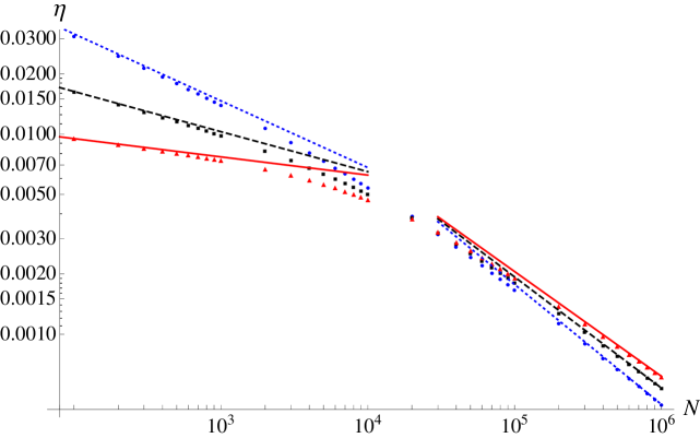
Figure 1: (Color online) $N$ dependence of the inverse volume $\eta_{N}$ in harmonic trap units. The points correspond to the results of the numerical integration of the 3D GP ground-state solution for different trap geometries: circles (blue) correspond to $q=2$, squares (black) to $q=4$, and triangles (red) to $q=10$. The respective Thomas-Fermi predictions for the 1D [Eq. (20)] and 3D regimes are the dotted (blue) line for $q=2$, dashed (black) line for $q=4$, and solid (red) line for $q=10$ labeling . The stiffness parameter $k$ of the trapping potential is chosen so that the crossover from 1D to 3D behavior occurs at $\bar{N}_{T}\simeq 14\,000$ for all three values of $q$.

From the numerical evaluation of $\eta_{N}$, it is straightforward to determine the exact scaling of $\delta\gamma_{1}$ with the number of atoms in the condensate and thus verify that in all cases it is better than $1/N$.

III.2 Ramsey fringes

The dynamics of the two-mode ⁸⁷Rb BEC we consider here is well described by a mean-field approach which neglects the entanglement and associated phase diffusion generated by the $\hat{J}_{z}^{\,2}$ interaction mertes07a ; anderson09 . In this approximation, the wave functions for the two hyperfine levels evolve according to the time-dependent, coupled, two-mode GP equations

$$i\hbar\frac{\partial\psi_{N,\alpha}}{\partial t}=\Biggl{(}-\frac{\hbar^{2}}{2m}\nabla^{2}+V+\sum_{\beta=1}^{2}g_{\alpha\beta}N_{\beta}|\psi_{N,\beta}|^{2}\Biggr{)}\psi_{N,\alpha},\quad\alpha=1,2,$$ (22)

which take into account the effect of the different scattering processes on the evolution of each mode wave function note1 . Here $N_{1}$ and $N_{2}$ denote the respective (mean) populations of levels 1 and 2.

We simulate the Ramsey interferometry scheme presented in Sec. II.2 as follows. Assuming that the atoms can be prepared in the superposition state $\psi_{N}(\vec{r})(|1\rangle+|2\rangle)/\sqrt{2}$ with unit fidelity, we first integrate Eq. (1) to find $\psi_{N}(\vec{r})$ and then evolve it for a time $t$ according to the coupled, three-dimensional GP equations (22) for the different potentials (13)xmds . Finally, supposing that the detection procedure can be considered instantaneous, we find the spatial overlap of the computed two-mode wave functions, $\psi_{N,1}(\vec{r},t)$ and $\psi_{N,2}(\vec{r},t)$, which modulates the detection probabilities $p_{1,2}(t)$ of Eq. (9) note2 .

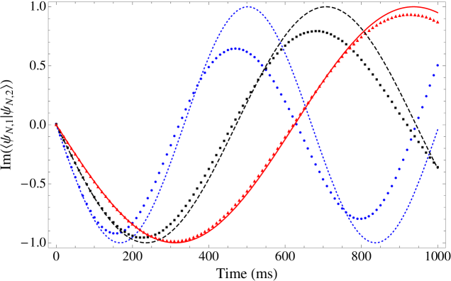
Figure 2: (Color online) Ramsey fringes for a cigar-shaped ⁸⁷Rb BEC of 1 000 atoms (labeling convention as in Fig. 1 labeling ). The points represent the numerical results of the integration of the coupled, two-mode, three-dimensional GP equations (22) for the different trapping potentials (13), whereas the lines are the respective idealized Josephson-approximation predictions (10), with the value of $\eta_{N}$ supplied by the numerics of Sec. III.1. The Josephson approximation improves as the trap gets harder.

Figure 2 shows the resulting Ramsey fringe pattern for a BEC of 1 000 atoms, as well as the idealized, Josephson-approximation fringe pattern (10), in which we use the numerical value of $\eta_{N}$ found for the potentials (13), as described in Sec. III.1. The agreement between the idealized fringe pattern and the numerical results for the tenth-order potential is quite remarkable in view of the complete neglect of spatial evolution by the Josephson approximation. As $q$ decreases or time increases, however, the simulated fringe pattern clearly deviates from the simplified dynamics described by the Josephson approximation. Such discrepancy reveals, in fact, the breakdown of the Josephson approximation.

The breakdown of the Josephson approximation becomes more evident in the case of 5 000 atoms shown in Fig. 3. Due to the difference in the scattering lengths and the scattering potentials, each wave function has a complex nonlinear evolution that, except for short times, can no longer be approximated as no evolution at all, as is assumed by the Josephson approximation. The short-time behavior can be better seen in Fig. 4, where we plot the Ramsey fringes for up to 120 ms. For longer times, the wave functions differentiate spatially, which leads to the reduction in fringe visibility and the change in the fringe frequency seen in Figs. 2 and 3. For $q=2$ and 5 000 atoms, the fringe pattern is already entering a revival before 1 s. The fringe visibility is clearly better preserved by going to a harder trap.

Figure 3: (Color online) Ramsey fringes for a cigar-shaped ⁸⁷Rb BEC of 5 000 atoms (labeling convention as in Fig. 1 labeling ). The points represent the numerical results of the integration of the coupled, two-mode, three-dimensional GP equations (22) for the different trapping potentials (13), whereas the lines are the respective idealized, Josephson-approximation predictions (10). Here we only plot the idealized fringe pattern (10) for short times, since it quickly deviates from the simulated nonlinear evolution; the deviation is a consequence of the differentiation of the wave functions of two modes as they evolve separately under the coupled GP equations. (Figure 4 shows a closeup of the first 120 ms.)

It is worth emphasizing that our results indicate that the integrated phase shift that we are interested in detecting is accumulated more rapidly than the time scale for the two wave functions to differentiate spatially. Moreover, for the regimes we consider and in view of typical Ramsey pulses and detection times ($\lesssim 1\,$ms) matthews98a ; mertes07a ; anderson09 , our simulations confirm that the Josephson model holds for a length of time that is sufficient to implement the metrology scheme.

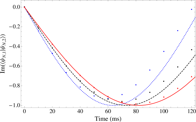
Figure 4: (Color online) Closeup of Fig. 3 for the first 120 ms. The Josephson approximation improves as the trap gets harder.

In the following section, we analyze an alternative analytical model, proposed in boixo09 , which attempts to provide a better description of the nonlinear detection signal shown in Figs. 2 and 3, by allowing the wave functions to accumulate a position-dependent phase shift.

IV Differentiation of the spatial wave functions

As already pointed out in the previous section, the distinct scattering lengths of the allowed $s$-wave collisions for the ⁸⁷Rb atoms ultimately make each wave function evolve differently in a nontrivial way colson78 . In fact, it is known that due to the interspecies repulsion, the two modes tend to separate spatially matthews98a . Before the modes segregate, however, the effect of the different nonlinearities is to produce a relative phase between the two modes that depends on the local density within the condensate.

All these phenomena have recently been observed in a ground-breaking set of experiments. In anderson09 , Anderson et al. measured the position-dependent phase shifts in the same two-mode ⁸⁷Rb BEC that we consider here, whereas Mertes et al. mertes07a demonstrated the nonequilibrium separation dynamics of the binary superfluid. The details of both experiments were shown to be well accounted for by numerical integrations of the coupled, two-mode GP equations (22), with an additional phenomenological loss term included.

In short, the two-mode dynamics can be explained as follows. For short times, the integrated part of the relative phase, which corresponds to the average difference in the energies of the scattering processes, is the dominant dynamical effect and provides the signal for our measurement protocol. The residual position-dependent part of the relative phase affects the two-mode dynamics on a somewhat longer time scale and reduces the visibility of the interference fringes on which the detected signal relies. Eventually, the position-dependent phases drive differences between the atomic densities associated with the two hyperfine levels, and this leads to spatial separation of the two modes.

The above-described effects occur on different time scales, which were estimated in boixo09 to be sufficiently different that the metrology protocol could be successfully implemented. The analytical estimates suggest that making the longitudinal trap harder leads to a greater separation of these three time scales. In order to retain good fringe visibility, the required operation time scale of the protocol was estimated to be well within the first fringe, which we can confirm from our simulations and is illustrated in Figs. 2 and 3.

In an attempt to model the complex dynamics of the two-mode condensate, we modify our analytical description by allowing the spatial wave functions to acquire a position-dependent phase shift in addition to the uniform phase shift of the Josephson approximation. Since the spatial segregation of the modes occurs on a longer time scale than the accumulation of a position-dependent phase shift, it is not relevant to this discussion. Moreover, for the regimes that concern us, we can include the position-dependent phase shift in a quite straightforward way. As before, we limit our analysis to the trapping potentials (13) and to quasi-1D BECs. In addition, considering our numerical simulations, we focus on the particular case of both modes being equally populated, although a more general discussion can be found in boixo09 .

As in the case of the ground state of a single-mode BEC in the one-dimensional regime, which was discussed in Sec. III.1, the wave functions of the two modes can be approximated by the product of transverse and longitudinal wave functions,

$$\psi_{N,\alpha}(\rho,z,t)=e^{-i\omega_{T}t}\chi_{0}(\rho)\phi_{N,\alpha}(z,t),\quad\alpha=1,2,$$ (23)

where $\chi_{0}$ is the previously defined time-independent, Gaussian ground state in the transverse dimensions. The longitudinal wave functions satisfy the time-dependent, coupled, longitudinal GP equations

$$i\hbar\frac{\partial\phi_{N,\alpha}}{\partial t}=\biggl{(}-\frac{\hbar^{2}}{2m}\frac{d^{2}}{dz^{2}}+\frac{1}{2}kz^{q}+\frac{1}{2}N\eta_{T}\sum_{\beta}g_{\alpha\beta}|\phi_{N,\beta}|^{2}\biggr{)}\phi_{N,\alpha},$$ (24)

where we have used our assumption that $N_{1}=N_{2}=N/2$.

For the traps and atom numbers that we are considering, it is legitimate to ignore the kinetic-energy terms in Eq. (24) boixo09 , as is done in the 1D Thomas-Fermi approximation. Within this approximation, the probability densities do not change with time, i.e.,

$$|\phi_{N,\alpha}(z,t)|^{2}=|\phi_{N}(z,0)|^{2}\equiv q_{0}(z),$$ (25)

with $|\phi_{N}(z,0)|^{2}$ given by Eq. (18); hence the evolution under the coupled GP equations simply introduces a phase that depends on the local atomic linear density,

$$\phi_{N,\alpha}(z,t)=\sqrt{q_{0}(z)}\exp\!\bigg{[}-\frac{it}{\hbar}\bigg{(}\frac{1}{2}kz^{q}+\frac{1}{2}N\eta_{T}q_{0}(z)\sum_{\beta}g_{\alpha\beta}\bigg{)}\bigg{]}.$$ (26)

This yields an overlap

$$\langle\psi_{N,2}|\psi_{N,1}\rangle=\langle\phi_{N,2}|\phi_{N,1}\rangle=\int dz\,q_{0}(z)e^{-i\delta\theta(z)},$$ (27)

where the position-dependent differential phase shift is given by

$$\delta\theta(z)=\frac{q_{0}(z)N\eta_{T}\gamma_{1}\,t}{\hbar}=\Omega_{N}t\left(1+\frac{q_{0}(z)-\eta_{L}}{\eta_{L}}\right)\;.$$ (28)

Here

$$\eta_{L}\equiv\int dz\,q_{0}^{2}(z)=\frac{q}{2q+1}\left(\frac{q+1}{q}\right)^{q/(q+1)}\left(\frac{k}{Ng_{11}}\right)^{1/(q+1)}\left(2\pi\rho_{0}^{2}\right)^{1/(q+1)},$$ (29)

and we have separated out the integrated phase shift $\Omega_{N}t$, whose angular frequency (11) is defined as in the Josephson approximation. This makes it clear that the residual position-dependent phase shift adds a correction to the integrated phase shift that we have previously calculated.

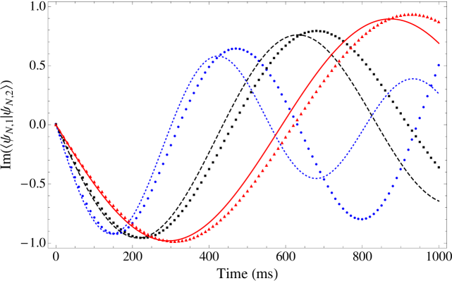
Figure 5: (Color online) Same as Fig. 2 (1 000 atoms), but here the lines correspond to the improved analytical prediction (30) for the three different values of $q$ (labeling convention as in Fig. 1 labeling ). The improved model succeeds in predicting a reduction in fringe visibility as time increases, but it does not give a better estimate of the fringe frequency.

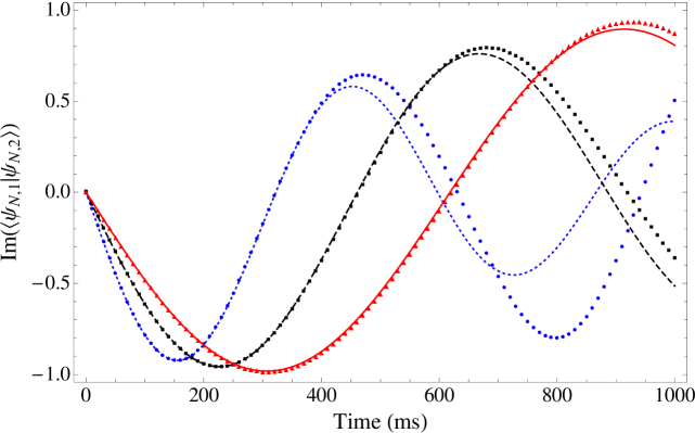
Figure 6: (Color online) Same as Fig. 2 (1 000 atoms), but here the lines correspond to the improved analytical overlap (30), computed using the numerically computed $\eta_{N}$ from Sec. III.1, as described in the text, for the three different values of $q$ (labeling convention as in Fig. 1 labeling ). The improved model, with the ad hoc use of the numerically computed $\eta_{N}$, provides a reasonably good account of the fringe frequency and of the reduction in fringe visibility as time increases, with better agreement for short times and for harder traps.

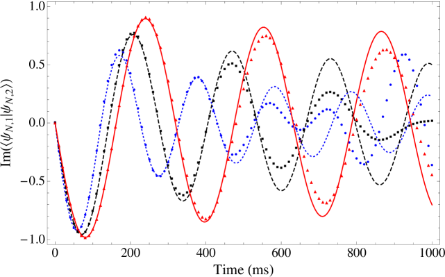
Figure 7: (Color online) Same as Fig. 3, but here the lines correspond to the improved analytical overlap (30), computed using the numerically computed $\eta_{N}$ from Sec. III.1, for the three different values of $q$ (labeling convention as in Fig. 1 labeling ). The improved model, with the ad hoc use of the numerically computed $\eta_{N}$, is surprisingly good even in the third fringe period for $q=10$.

Putting all this together, we can write the overlap as

$$\langle\psi_{N,2}|\psi_{N,1}\rangle=\int dz\,q_{0}e^{-iq_{0}N\eta_{T}\gamma_{1}\,t/\hbar}=e^{-i\Omega_{N}t}\int dz\,q_{0}e^{-i\Omega_{N}t(q_{0}-\eta_{L})/\eta_{L}},$$ (30)

whose imaginary part, as before, is responsible for the fringe pattern in our interferometry scheme. In Fig. 5, we compare the numerical fringes with the imaginary part of the overlap (30) for 1 000 atoms. We do exactly as the current approximation instructs: we use the longitudinal Thomas-Fermi probability density $q_{0}(z)$, the corresponding $\eta_{L}$ from Eq. (29), and the transverse $\eta_{T}$ from the transverse ground state $\chi_{0}$ [Eq. (16)]. The improved model captures an approximation to the reduction in fringe visibility, with agreement with the numerics getting better as $q$ increases, but it predicts a fringe frequency that is too large. Indeed, by comparing Fig. 5 to Fig. 2, one sees that the frequency of the improved model is too high by an amount that is somewhat larger than the amount by which the Josephson approximation’s frequency is too low.

It is not hard to identify a source for this frequency disparity. The current approximation uses an atomic density profile that comes from the product wave function (23), with the longitudinal wave function coming from Eq. (26) and the transverse wave function assumed to be the $N$-independent Gaussian ground state of the transverse harmonic trap. In contrast, the frequency $\Omega_{N}$ we use in the Josephson-approximation plots of Figs. 2 and 3 comes from numerical computation of the 3D GP ground state.

We can test whether this is a source of the frequency disparity by making an ad hoc adjustment to the model of this section. In particular, in using the analytical overlap (30), we can use the longitudinal Thomas-Fermi probability density $q_{0}(z)$ and its $\eta_{L}$ from Eq. (29), as the approximation instructs. We could instead adopt the ad hoc procedure of using the numerically computed $\eta_{N}$ plotted in Fig. 1; the transverse $\eta_{T}$ determined in this procedure from $\eta_{T}=\eta_{N}/\eta_{L}$ , is no longer that of the transverse ground state and acquires an $N$ dependence from $\eta_{N}$ and $\eta_{L}$.

In Figs. 6 and 7, we compare the numerical fringes with the imaginary part of the overlap (30), computed using the ad hoc modification, for 1 000 and 5 000 atoms. The improved model, with this ad hoc adjustment, is surprisingly good at predicting both the fringe frequency and the reduction in fringe visibility, especially for $q=10$ (the Josephson-approximation fringes would have the same frequency discrepancy had we used the 1D Thomas-Fermi approximation and the transverse ground state to determine $\eta_{N}$, instead of using the numerical value). We emphasize that the fringe visibility is preserved better by going to harder traps. Within the improved model, it is clear that the better fringe visibility of harder traps is due to the fact that as $q$ increases, the trapping potential becomes more flat-bottomed, making the atomic density profile more uniform across the trap and and thus reducing the size of the residual position-dependent phase shift.

It is clear that our improved analytical model does indeed provide a more accurate description of the nonlinear evolution of the two-mode condensate and consequently of the fringe pattern of our protocol. Notice, however, that for longer times effects that are not considered in this model, such as mode segregation, become significant and, therefore, the Ramsey fringes can no longer be described by Eq. (30). As already noted, for $q=2$ and 5 000 atoms, the nonlinear evolution is undergoing a revival well before $t=1\,$s, an effect that cannot be described within our model.

Throughout this analysis we consider the case of a one-dimensional BEC whose ground-state wave function is supposed to be well approximated by the product ansatz (14). In this approximation one assumes that the effect of the scattering interaction on the transverse degrees of freedom of the gas can be completely neglected. As we discuss in Sec. III.1, this is a good approximation as long as the number of atoms in the condensate is small compared to the critical atom number $\bar{N}_{T}$. In fact, from Fig. 1 one sees that as $N$ approaches $\bar{N}_{T}$, the product wave function (14) fails to give an accurate estimate of the inverse volume $\eta_{N}$.

The main reason for this discrepancy is that as $N$ approaches the critical atom number $\bar{N}_{T}$, the condensate begins to spread in the transverse dimensions. Indeed, the analysis in this section shows that we obtain a reasonably good account of the fringe signal by including a position-dependent phase shift to describe the reduction in fringe visibility and by allowing $\eta_{T}$ to change with $N$ as dictated by the numerical 3D ground-state wave function, thus reflecting the spreading of the condensate in the transverse dimensions.

V Conclusion

We present in this paper a detailed numerical analysis of a recent proposal of a Ramsey interferometry scheme that takes advantage of the nonlinear scattering interactions in a two-mode ⁸⁷Rb Bose-Einstein condensate to achieve detection sensitivities that scale better than the $1/N$ limit of linear metrology boixo08b . In view of current experimental techniques and typical parameters, this scheme is a feasible proof-of-principle experiment that in terms of sensitivity scaling, can outperform Heisenberg-limited linear interferometry. The proposed protocol does not rely on complicated state preparation or measurement schemes nor on entanglement generation to enhance the measurement sensitivity.

We first analyze here how the scaling is affected by the expansion of the atomic cloud as a function of the number of atoms in the condensate and of the geometry of the trap, by considering the case of quasi-1D BECs trapped by different potentials. Later we find the exact dependence of the atomic density with the atom number $N$, solving numerically the single-mode, three-dimensional GP equation. This allows us to pin down the exact scaling and to verify that in all the considered cases a scaling better than $1/N$ can be achieved.

In addition, we simulate the proposed interferometric scheme and the corresponding measurement signal by solving the two-mode, coupled, three-dimensional GP equations. Our numerical results not only confirm the theoretical predictions derived in boixo09 , but also show that the assumption that the two modes share the same spatial wave function is justified for a length of time sufficient to run the metrology scheme. For longer times, it becomes evident that the Josephson Hamiltonian (5) is unable to handle the full two-mode dynamics because it ignores entirely the spatial evolution of the condensate wave functions.

To get a more accurate description of the fringe signal, one needs to take into account the spatial differentiation of the wave functions of the two modes. We formulate an improved model that partially describes the differentiation of the wave functions by including a position-dependent phase shift across the condensate. This model, based on a one-dimensional Thomas-Fermi approximation, gives a considerably refined account of the fringe signal of our protocol.

Our analysis shows that as the number of atoms in the condensate approaches the critical atom number $\bar{N}_{T}$, deviations of the assumed product wave function from the numerically computed initial condensate wave function result in less accurate analytical estimates of the oscillation frequency of the fringe pattern. Preliminary results indicate, however, that this effect can be described by means of perturbative techniques, which treat the scattering interaction as a perturbation to the single-particle transverse Hamiltonian and which will be presented elsewhere. The perturbation theory indicates that there should be corrections to the product wave function as well. For more hard-walled and flat-bottomed potentials, we find that corrections to our idealized models become less important, confirming that one should consider potentials such as boxes or rings as the preferred architectures for nonlinear BEC metrology.

- (1) V. Giovannetti, S. Lloyd, and L. Maccone, Phys. Rev. Lett. 96, 010401 (2006).
- (2) A. Luis, Phys. Lett. A 329, 8 (2004).
- (3) S. Boixo, A. Datta, S. T. Flammia, A. Shaji, E. Bagan, and C. M. Caves, Phys. Rev. A 77, 012317 (2008).
- (4) S. Boixo, A. Datta, M. J. Davis, S. T. Flammia, A. Shaji, and C. M. Caves, Phys. Rev. Lett. 101, 040403 (2008).
- (5) M. J. Woolley, G. J. Milburn, and C. M. Caves, New J. Phys. 10, 125018 (2008).
- (6) S. Boixo, A. Datta, M. J. Davis, A. Shaji, A. B. Tacla, and C. M. Caves, Phys. Rev. A 80, 032103 (2009).
- (7) S. Boixo, S. T. Flammia, C. M. Caves, and J. M. Geremia, Phys. Rev. Lett. 98, 090401 (2007).
- (8) A. M. Rey, L. Jiang, and M. D. Lukin, Phys. Rev. A 76, 053617 (2007).
- (9) S. Choi and B. Sundaram, Phys. Rev. A 77, 053613 (2008).
- (10) F. Dalfovo, S. Giorgini, L. P. Pitaevskii, and S. Stringari, Rev. Mod. Phys. 71, 463 (1999).
- (11) A. J. Leggett, Rev. Mod. Phys. 73, 307 (2001).
- (12) K. M. Mertes, J. W. Merrill, R. Carretero-Gonzalez, D. J. Frantzeskakis, P. G. Kevrekidis, and D. S. Hall, Phys. Rev. Lett. 99, 190402 (2007).
- (13) C. M. Dion and E. Cancès, Comp. Phys. Comm. 177, 787 (2007).
- (14) G.-B. Jo, J.-H. Choi, C. A. Christensen, Y.-R. Lee, T. A. Pasquini, W. Ketterle, and D. E. Pritchard, Phys. Rev. Lett. 99, 240406 (2007).
- (15) All the plots in this paper share the following labeling conventions: points represent numerical data for the different trapping potentials (13), with circles (blue) corresponding to , squares (black) to , and triangles (red) to ; corresponding analytical expressions are plotted as lines: dotted (blue) for , dashed (black) for and solid (red) for .
- (16) R. P. Anderson, C. Ticknor, A. I. Sidorov, and B. V. Hall, Phys. Rev. A 80, 023603 (2009).
- (17) It is noteworthy that the coupled GP equations include a linear approximation to , which corresponds to setting , which should be valid for short times. Notice that because we consider the populations of the two modes to be the same, it follows that .
- (18) To solve the coupled two-mode GP equations numerically, we use the code generator XmdS, available at www.xmds.org.
- (19) In our simulations we assume that one can neglect the evolution of the spatial modes during the Ramsey pulses. According to matthews98a ; mertes07a ; anderson09 , the two hyperfine levels of 87Rb can be coupled by two-photon Rabi pulses whose duration is of the order of 1 ms, which is much faster than the characteristic time for the condensate to change its shape, thereby justifying such an approximation.
- (20) M. R. Matthews, D. S. Hall, D. S. Jin, J. R. Ensher, C. E. Wieman, E. A. Cornell, F. Dalfovo, C. Minniti, and S. Stringari, Phys. Rev. Lett. 81, 243 (1998).
- (21) W. B. Colson and A. L. Fetter, J. Low Temp. Phys. 33, 231 (1978).