Non-universality of halo profiles and implications for dark matter experiments

Abstract

We explore the cosmological halo-to-halo scatter of the distribution of mass within dark matter halos utilizing a well-resolved statistical sample of clusters from the cosmological Millennium simulation. We find that at any radius, the spherically-averaged dark matter density of a halo (corresponding to the “smooth-component”) and its logarithmic slope are well-described by a Gaussian probability distribution. At small radii (within the scale radius), the density distribution is fully determined by the measured Gaussian distribution in halo concentrations. The variance in the radial distribution of mass in dark matter halos is important for the interpretation of direct and indirect dark matter detection efforts. The scatter in mass profiles imparts approximately a 25 percent cosmological uncertainty in the dark matter density at the Solar neighborhood and a factor of $\sim$3 uncertainty in the expected Galactic dark matter annihilation flux. The aggregate effect of halo-to-halo profile scatter leads to a small (few percent) enhancement in dark matter annihilation background if the Gaussian concentration distribution holds for all halo masses versus a 10 percent enhancement under the assumption of a log-normal concentration distribution. The Gaussian nature of the cluster profile scatter implies that the technique of “stacking” halos to improve signal to noise should not suffer from bias.

1 introduction

Overwhelming evidence indicates that most of the mass in the Universe is composed of dark matter. In the concordance $\Lambda$ Cold Dark Matter ($\Lambda$CDM) cosmological model, structure formation is dominated by the gravitational evolution of dark matter. At the present epoch, most of the mass has been assembled into self-bound halos, which are hosts to the galaxies, clusters, and groups that are observed. Although the exact nature of dark matter is unknown, theoretically motivated extensions to the standard model of particle physics suggest cold dark matter candidates which were in thermal equilibrium in the early Universe and interact only weakly with baryonic matter.

Weakly Interacting Massive Particles (WIMPs) are ideal dark matter candidates as they arise naturally in many extensions of the standard model of particle physics. The strength of their interactions can mimic the physical behaviour of the dark matter (weak as well as gravitational) inferred from a broad range of observations. WIMP dark matter candidates have a small but non-zero cross-section for self-annihilation (Jungman, Kamionkowski & Griest 1996). Indirect detection experiments look for the by-products of this annihilation, typically in the form of high-energy photons, neutrinos and positrons, as well as low-energy antiprotons (see Jungman, Kamionkowski & Griest 1996; Bertone, Hooper & Silk 2005).

In recent years, halo structure has been widely explored using cosmological numerical simulations. Pioneering work by Navarro, Frenk & White (1996, 1997; NFW hereafter) used numerical simulations to show that the spherically-averaged radial density profile of dark matter halos is approximately “universal”. However, NFW and later Jing (2000) and Bullock et al. (2001) noted significant variations in the profile between different halos, in that some are better fit by steeper (higher concentration) profile forms than others. These variations were shown to be correlated with halo formation time (e.g. Wechsler et al. 2002). Upon close inspection, the profile of any individual halo cannot be described by any particular smooth functional form (e.g. Jing 2000; Reed et al. 2005; Gao & White 2006; Knollmann, Power & Knebe 2008; Lukić et al. 2009). In this sense, the halo mass profile is not truly “universal”. Thus, due to this fundamentally non-smooth nature of the radial mass distribution of halos, functional forms do not provide a complete and accurate description of the halo density.

In this paper, we quantify the mean and scatter of the halo radial mass distribution without the a priori assumption of a smooth functional form. We use a large sample of halos extracted from the “Millennium” cosmological numerical simulation, whose combination of large volume and fine mass resolution are ideal for studying statistical variations in halo mass profiles. Our approach begins with an empirical non-parametric measure of the distribution function of halo densities, allowing us to include the effects of halo-to-halo and intra-halo non-universality in addition to effects relating to scatter in halo concentrations. We focus on small radii where the “smooth” dark matter component dominates the mass distribution; here, self-bound satellite “subhalos” are deficient because of efficient tidal stripping before reaching small radii (Springel et al. 2008). This allows us to quantify the cosmological scatter in the smooth component of the dark matter density. We apply our results to several cosmological applications, including direct and indirect experimental efforts of dark matter detection.

Annihilation of dark matter scales as the square of the number density of particles, and thus any detected annihilation signal will be sensitive to the precise distribution of dark matter. Past work focused on using extremely high resolution simulations of individual dark matter halos of Galactic mass to estimate annihilation luminosities for particular dark matter candidates (Kuhlen, Diemand & Madau 2008; Springel et al. 2008). These impressive numerical simulations were able to quantify the level at which substructure contributes to the annihilation signal, as well as get a glimpse of the phase-space structure of the Milky Way halo at the Solar neighbourhood. However, halo-to-halo variations in the radial mass profile implies a “cosmological” uncertainty in the predicted annihilation rate in halos, which is of course in addition to the uncertainties related to the mass, cross-section, and other properties of the dark matter particle.

Dark matter annihilation in halos produces a cosmological background whose strength depends upon the numbers of halos throughout the history of the Universe and their density profiles (e.g. Ullio et al. 2002; Zavala, Springel & Boylan-Kolchin 2010). When integrated over all halos, a scatter in halo density profiles implies a boost of the annihilation background with respect to the case where all halos follow a universal profile without scatter (e.g. Ullio et al. 2002). The strength of the annihilation background will thus be sensitive to both the average and the scatter in halo dark matter profiles. Inferring the dark matter particle mass and cross section from a background annihilation signal will thus require separating out the integrated effects of cosmological scatter.

In addition, even within the Milky Way, interpretation of both direct and indirect dark matter detection efforts requires an understanding of the intrinsic variance in halo profiles. The cosmological uncertainty in the local dark matter density at the solar radius is essential in the interpretation of a detection (or lack of) in direct detection experiments. In particular, knowledge of the intra-halo scatter in density with radius is needed to evaluate results of direct (local) dark matter detection efforts in the context of indirect (non-local) detection experiments focussed on the Galactic center or elsewhere. Thus, both direct and indirect dark matter detection efforts face the challenge of disentangling the influences of cosmological halos from the properties of the dark matter particle.

In this paper, we use a large number of cosmological halos to quantify the cosmological variance in halo densities, and to assess the level at which the distribution of halo densities affects the interpretation of dark matter direct and indirect detection experiments. In § 2, we review the general characteristics of dark matter halo mass distribution, and we give an overview of the cosmological simulations that we use in § 3. We present our analysis of the mass distribution and its scatter within halos in the simulation in § 4, showing that the distribution of halo concentrations yields an accurate description of the measured scatter of the smooth component of dark matter within halos. We apply our findings to experimental searches of dark matter in § 5; we discuss limitations of our work (§ 6), followed by a brief conclusion (§ 7).

2 The dark matter halo profile

As a baseline reference for examining the cosmological scatter of halo density profiles, it is convenient to parameterize the density profile by a spherically-averaged functional form. Recent works favor the Einasto (1965) profile form as a description of cosmological halos (Navarro et al. 2004; Gao et al. 2008; Hayashi & White 2008). In this case, the logarithmic slope of the density is a simple power-law:

$${d\ln\rho\over d\ln r}=-2\left({r\over r_{-2}}\right)^{\alpha}.$$ (1)

The “scale radius”, $r=r_{-2}$, has a density slope of $-2$, and defines the halo concentration as:

$${c_{vir}=\frac{r_{vir}}{r_{-2}},~{}{\rm or}~{}c_{200}=\frac{r_{200}}{r_{-2}}},$$ (2)

where in the first definition, $r_{vir}$ is the virial radius of the halo, defined as a sphere of 95.4 times critical density (Eke, Cole, & Frenk 1996), while in the second definition, $r_{200}$ is the radius where the enclosed density is 200 times the critical density of the Universe. The parameter $\alpha$ in Eq. 1 varies weakly with mass and redshift. On average $\alpha=0.19$, for $z=0$ clusters over the mass range that we explore (as shown in Gao et al. 2008). Density is given by:

$$\rho(r)=\rho_{-2}\exp\left\{-\frac{2}{\alpha}\left[\left(\frac{r}{r_{-2}}\right)^{\alpha}-1\right]\right\}.$$ (3)

The normalization of the profile is obtained from requiring that the mass of the halo is $M=\int_{0}^{R_{200}}4\pi\rho(r)r^{2}dr$, thus

$$\rho_{-2}=\frac{2^{3/\alpha}c_{200}^{3}M}{4\pi\,e^{2/\alpha}\alpha^{(3-\alpha)/\alpha}R_{200}^{3}\left[\Gamma\left(\frac{3}{\alpha}\right)-\Gamma\left(\frac{3}{\alpha},\frac{2c_{200}^{\alpha}}{\alpha}\right)\right]}.$$ (4)

Here, $\Gamma(x)$ and $\Gamma(x,y)$ are the Gamma, and Incomplete Gamma functions respectively.

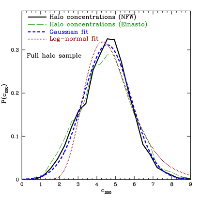
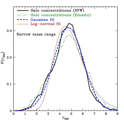
Figure 1: Left panel: The probability distribution function (PDF) of concentrations for the 3,501 halos with $M\geq 8.6\times 10^{13}h^{-1}M_{\odot}$ shown against best-fit Gaussian with a mean $\langle c\rangle=4.55$, and standard deviation $\sigma_{c}=1.28$. This provides a better match than the best-fit log-normal distribution with a mean $\langle\log_{10}c\rangle=0.669$ and a standard deviation in $\log c$ of $\sigma_{\log c}=0.121$. Concentration fits made to the NFW profile produce a modestly narrower distribution, even though the Einasto profile is overall a better description of the halo mass distribution. Right panel: The distribution of concentrations in a narrow virial mass range of $8.6\times 10^{13}\leq[M/h^{-1}M_{\odot}]\leq 1.7\times 10^{14}$ (2,276 halos). The shape of the concentration PDF remains Gaussian.

3 Simulations and halo catalogue

We utilize the gravity-only N-body particle Millennium Simulation of Springel et al. (2005). This simulation evolves 2160³ particles in a periodic box of 500$h^{-1}$Mpc using the gravity solver code lgadget2 (Springel et al. 2005), a modified version of the publicly available gadget2 (Springel 2005). Particle mass is $8.6\times 10^{8}h^{-1}M_{\odot}$. The cosmological parameters used are $\Omega_{m}=0.25$, $\Omega_{\Lambda}=0.75$, hubble constant $h=0.73$, $\Omega_{b}=0.045$, $n=1$, with power spectrum normalization $\sigma_{8}=0.9$. The matter power spectrum used to create initial conditions is produced using CMBFAST (Seljak & Zaldarriaga 1996).

For this study, it is important to use as large a statistical sample of halos as possible. In addition, these halos must be resolved in the innermost regions in which we are interested. We thus consider all halos with more than 10⁵ particles, corresponding to $M_{vir}\geq 8.6\times 10^{13}h^{-1}M_{\odot}$. This results in 3,501 halos. The density profiles for these halos are resolved down to $\sim 1-2\%r_{vir}$, based on convergence tests in Moore et al. (1998), Power et al. (2003), and Reed et al. (2005) for halos with similar numbers of particles.

We define halos and their centers using the same procedure as was done in Neto et al. (2007) and Gao et al. (2008). Halos are identified initially using friends-of-friends with linking length of 0.2 times the mean inter-particle spacing. Halos are centered on the location of the deepest potential of the main subhalo. Halo mass is then determined by a sphere of 95.4 times critical density ($M_{vir}$), and additionally by a sphere of 200 times critical density ($M_{200}$). We determine a spherically-averaged logarithmically binned density profile for each halo.

4 Cosmological Variations in the Halo Profile

In this section we discuss the cosmological variance in the properties that describe the profile of dark matter halos.

4.1 Halo Concentrations

Halo concentrations have been shown to have significant halo-to-halo scatter, with a median that decreases with increasing mass and redshift (e.g. Bullock et al. 2001; Neto et al. 2007; Gao et al. 2008; Duffy et al. 2008; Maccio et al. 2008). Early work suggested that the distribution of halo concentrations is log-normal (Jing 2000; Bullock et al. 2001). However, larger samples of higher resolution halos reveal significant departures from a log-normal scatter, primarily due to a tail of low concentrations inferred from “unrelaxed” halos (Neto et al. 2007; Maccio et al. 2008), which tend to conform poorly to smooth functional fits (Lukić et al. 2009). In fact, the distribution of halo concentrations is very well described by a simple Gaussian, as noted by Lukić et al. (2009), when all (relaxed and unrelaxed) halos are considered. In Fig. 1 we show the concentration probability distribution function (PDF) from our full sample. We find that a Gaussian description of concentrations is a better fit than a log-normal distribution to the halos in our sample. More complicated functional descriptions of halo concentrations such as that suggested by Neto et al. (2007) or by Maccio et al. (2008) appear unnecessary to describe our data (which consists of the high mass halo subset of the halos of Neto et al. 2007 and Gao et al. 2008).

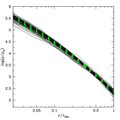
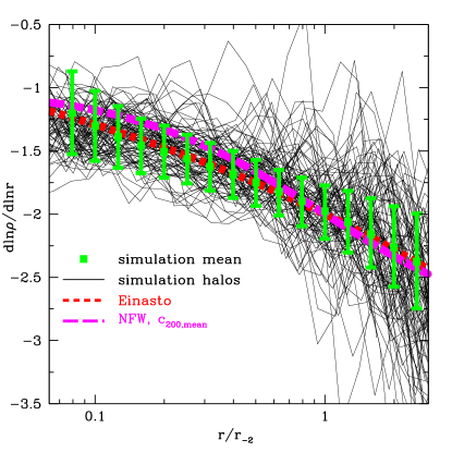
Figure 2: Left panel: Density profiles for 100 random halos from the sample. Points with error bars denote the mean and the $1\sigma$ scatter of the distribution for the full halo sample. Right panel: Logarithmic density slope for the 100 largest halos. Slopes are normalized to the scale radius to remove the effect of scatter in halo concentrations. An Einasto profile with $\alpha=0.19$ is a good match to the mean simulation slope.

In estimating halo concentrations, we consider both the Einasto profile (Eq. 1-4) and the NFW profile (NFW 1996; 1997):

$$\rho={4\rho_{-2}\over(r/r_{-2})(1+r/r_{-2})^{2}}.$$ (5)

A concentration defined by the Einasto profile is, in principle, equivalent to that defined by the NFW profile, both having a scale radius at $r_{-2}$. However, because simulation halos tend to better match the Einasto form, which is steeper than NFW at the smallest radii, a concentration inferred from the NFW form can be biased high or low, depending on the range of radii used in fitting (see Gao et al. 2008). We find that although the Einasto profile produces a better fit to stacked halos, the distribution of concentrations is modestly narrower when fit according to an NFW profile (see Fig. 1), with approximately the same mean value ($c_{200,NFW}=4.55$ versus $c_{200,Einasto}=4.50$). The Einasto distribution remains wider, whether or not the Einasto parameter $\alpha$ is fixed or allowed to float as a free parameter in the fit. For this reason (and also for convenience), we determine halo concentrations by fitting the NFW profile (Eq. 5) in the remainder of this paper. We stress that the shape of the Einasto-fit distribution of concentrations is nearly identical to that of the NFW-fit concentration PDF; the only difference is that the Einasto-fit concentration PDF is slightly wider ($\sim 10\%$) Gaussian. Profiles are fit to logarithmic radial bins over a range of $0.05-1r_{200}$ with normalization set by the mass contained within $r_{200}$.

We have confirmed also that fixing the density normalization instead of allowing it to float as a fit parameter has no significant effect upon the derived concentrations. As a further test, we show that the relatively wide range in halo masses for our full sample does not affect the shape of the distribution of concentrations. With a narrower sample mass range of $2\times$ in mass ($8.6\times 10^{13}\leq[M_{vir}/h^{-1}M_{\odot}]\leq 1.7\times 10^{14}$), a Gaussian concentration distribution is still preferred over log-normal (right panel of Fig. 1). The similar shape for the narrower mass range is not surprising because the mass dependence on mean halo concentration is relatively weak; and more importantly, this shows that the shape of the concentration distribution is not sensitive to our choice of the width of the mass range for the halo sample used throughout the paper.

4.2 Halo Densities

It is important to note that the Einasto profile has been found to fit halos well for a “stacked” ensemble (e.g. Hayashi & White 2008; Gao et al. 2008). However, the presence of substructure and other peculiarities implies that any particular halo profile tends to have significant variations from this mean smooth function.

In the left panel of Fig.  2, we show this scatter in the density profile for 100 random halos. The spread in densities due to different concentrations is also apparent. The right panel of Fig. 2 shows that there is very large scatter in the logarithmic slope of the density profile, plotted here versus $r/r_{-2}$. This representation removes differences that arise due to concentration. The increased scatter in density slopes at outer radii is independent of mass within our sample (i.e. similar behavior is seen for the 100 least massive halos in the sample); large radii scatter is likely enhanced by large substructures. The mean slope of the complete halo sample is well described by an Einasto profile, and is poorly matched by an NFW profile.

In Fig. 3, we show the probability distribution function (PDF) of densities at various radii in spherically-averaged shells from the halo sample. The width of the halo-to-halo scatter of density decreases toward larger radii. A possible explanation for this radial trend results from the fact that the central structure of the halo is assembled at higher redshifts than the outer parts of the halo (see e.g. Fukushige, Kawai, & Makino 2004; Reed et al. 2005). If one assumes that halo density at a particular radius correlates with the mean density of the universe at the time of mass infall, then scatter in mass assembly redshift from halo to halo would yield density variations that would be larger nearer the center due to the $(1+z)^{3}$ evolution of the mean matter density. Note that, at all radii, the width of the distribution is small compared to the statistical measurement uncertainty, which is estimated from Poisson counting of particles in radial bins.

The halo density PDF is well-described by a Gaussian at each radius. As an example, in Fig. 4, we show the density distribution function at a radius of $r=0.03r_{200}$. This scatter in densities is primarily due to the distribution in halo concentrations rather than intra-halo departures from a smooth functional form (i.e. “bumps”). For small radii ($r\lower 2.15277pt\hbox{$\;\buildrel<\over{\sim}\;$}r_{-2}$), the Gaussian PDF of halo spherical shell densities is well-matched by assuming that each halo is described by a deterministic Einasto radial density profile whose concentration is drawn from a Gaussian distribution (see Fig. 4). This implies that the distribution of halo concentrations fully determine the PDF of the smooth density component, and provides additional support that the form of the concentration PDF is Gaussian. More specifically, the effect of radial density “bumps” within the halo cannot be larger than the effect of measurement uncertainty of individual halo concentrations. A log-normal concentration distribution is unable to reproduce the density distribution shape or peak. Unsurprisingly, an assumption of an NFW profile does not match the density peak, although it is able to produce the Gaussian shape and width.

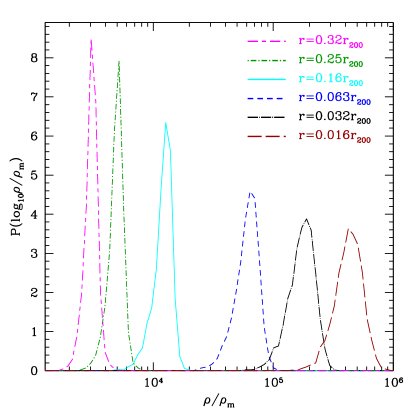
Figure 3: Halo-to-halo distribution in density at various radii relative to $r_{200}$ in the full halo sample. Densities are plotted in units of mean density of the universe, $\rho_{\rm m}$.

At larger radii ($r\lower 2.15277pt\hbox{\mbox{$\;\buildrel>\over{\sim}\;$}}r_{-2}$), the distribution remains Gaussian but is wider than implied by the distribution of concentrations, possibly due to increased scatter introduced from substructure or from a lower degree of relaxation in the outskirts of these recently formed cluster-size halos. The distribution of densities in our data is described to ($\sim 10\%$) accuracy by the following function:

$${\log_{10}\sigma_{\rho}=1.144\,\log_{10}\langle\rho\rangle-1.389},$$ (6)

where $\langle\rho\rangle$ and $\sigma_{\rho}$ are found via a Gaussian fit to the densities measured from the halo sample at a given radius. The agreement between the fit and the simulation data, shown in Fig. 5, over more than three orders of magnitude in density is interesting. However, we do not advocate that this is a universal function; further work is required to determine whether this relation between density and its scatter remains valid for lower halo masses and different redshifts. The moderate flattening of $\sigma_{\rho}$ at low density reflects the relative widening of the density PDF at large halo radii.

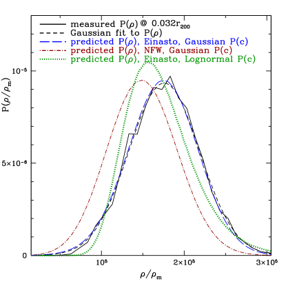
Figure 4: Measured density distribution at 0.032r₂₀₀, as an example, versus density distribution predicted by a deterministic Einasto profile and a Gaussian concentration distribution of width $\sigma_{c200}=1.28$, centered on $c_{200}=4.55$ to match the measured values of our sample. Log-normal concentration prediction assumes the best-fit to our sample of $\sigma_{log10c}=0.121$ with median $c=4.66$. Gaussian concentrations match the shape and peak position of the density distribution better than log-normal concentrations. Note that the concentration distribution for all curves comes from an NFW concentration fit (even when applied to the Einasto profile), which produces essentially equivalent concentrations to an Einasto-fit (see Fig. 1 and § 4.1); we use such NFW-derived concentrations here and hereafter.

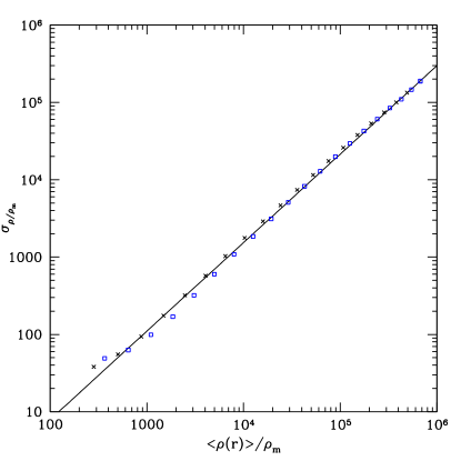
Figure 5: The width of the distribution of densities at various radii, $\sigma_{\rho}$, as determined by fitting a Gaussian, plotted as a function of mean density of our halo sample at each fitted radius for fixed $r/r_{vir}$ (black crosses) and for fixed $r/r_{200}$ (blue squares). The density distribution, $P(\rho)$, is well-described by a Gaussian distribution at all radii. Line is a fit given by Eq. 6.

It is instructive to consider also the distribution of halo density profile slopes. In Fig. 6, we show the distribution of the logarithmic radial slope of the density at various radii. The PDF of $d\ln\rho/d\ln r$ is well-described by a Gaussian distribution, except perhaps at large radii where substructure or other effects appear to result in wider than Gaussian tails. The mean of this distribution at each radius is consistent with the Einasto profiles with $\alpha=0.19$. Note that the Einasto profile with fixed $\alpha$ implies zero scatter in the PDF of halo slopes. The radii in the right panel of Fig. 6 are chosen such that they should have identical logarithmic slopes, assuming the Einasto profile, for the mean halo concentration of 4.55.

For most radii, the width of the distribution of slopes is similar whether measured in terms of $r_{-2}$ or in terms of $r_{200}$, apart from the innermost plotted radius. This is surprising because differences in halo concentrations should contribute to the spread in $d\ln\rho/d\ln r$ only at fixed $r/r_{200}$, and not at fixed $r/r_{-2}$, according to the Einasto (or NFW) self-similar profile form in which $d\ln\rho/d\ln(r/r_{-2})$ is independent of concentration. For this reason, we naively would have expected the spread in density slopes to be smaller at fixed $r/r_{-2}$ than at fixed $r/r_{200}$ (provided that $r_{-2}$ is determined accurately). This suggests that intra-halo “bumps” rather than halo concentration is the major contributor to scatter in the slope PDF. In fact, Eq. 1 implies that the distribution in density slopes at fixed $r/r_{200}$ due to the concentration distribution should be $\lower 2.15277pt\hbox{$\;\buildrel<\over{\sim}\;$}0.1$, which is much smaller than the actual spread which ranges from $0.17<\sigma_{d\ln\rho/d\ln r}<0.34$ at the fixed $r/r_{200}$ values shown.

At the smallest radius of $r_{-2}/10$, the slope distribution width is likely dominated by errors in the concentration measurement (left panel). Presumably for this reason, the PDF of the slopes is narrower when considered with respect to $r_{200}$ at the smallest radii. At each radius, we show an estimate of the uncertainty in the slope measurement, based on poisson noise from the average number of particles per radial bin. The slope uncertainty is significantly smaller than the measured PDF, except at the smallest plotted radius. Because numerical problems are most difficult to overcome at small radii, poisson uncertainty could underestimate the true error. We thus cannot rule out the possibility that the broadened PDF at small radii may have numerical origins. Indeed, increasing the minimum halo mass of the sample by a factor of 5 narrows the slope PDF at the smallest radii such that this effect is significantly smaller.

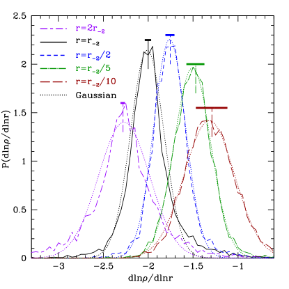
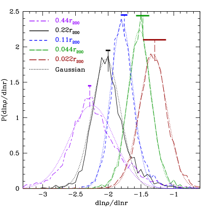
Figure 6: Distribution in halo slopes at various radii (solid lines) relative to the scale radius ($r_{-2}=r_{200}/c_{200}$) (left), and relative to $r_{200}$ (right). Dotted curves are best-fit Gaussians. Vertical lines denote the slope of the Einasto profile with $\alpha=0.19$. In the right panel, the Einasto profile slopes are shown for the mean halo concentration of 4.55. Slopes are reasonably fit by a Gaussian with an average consistent with the Einasto profile and a width that is narrowest near $r_{-2}$. Again, these concentrations (i.e. $r_{-2}$) are estimated from an NFW profile fit, which is essentially equivalent to a direct Einasto fit. Horizontal lines indicate an estimate of the slope measurement uncertainty.

5 Effects of profile scatter on dark matter annihilation

In this section we discuss the effect of the profile scatter on the expected signal in $\gamma$-rays (or other byproduct) from dark matter annihilation in halos.

In general, the total gamma-ray luminosity from a halo of mass $M$ is given by the volume integral of the square of its mass distribution as

$${\cal L}=\frac{\langle\sigma v\rangle}{M_{\chi}^{2}}\int_{0}^{R_{v}}\rho_{M}^{2}(r)d^{3},$$ (7)

where $M_{\chi}$ is the mass of the dark matter particle, and $\langle\sigma v\rangle$ is the thermal average of the annihilation cross section. Particle physics enters through the mass of the dark matter particle, and through its total annihilation cross section. As an example, in order to demonstrate the effects of density distributions on the annihilation flux, we consider a dark matter particle with mass $M_{\chi}=400{\rm GeV}$, with a total annihilation rate to $b\bar{b}$ quarks given by $\langle\sigma v\rangle=10^{-26}{\rm cm^{3}/s}$. We assume these values throughout the rest of this manuscript, and note that in general, the assumed dark matter particle properties affect the normalization of the results presented, and not the shape of the distributions.

The “dark luminosity” of a halo is determined by the distribution of its mass (see Eq. 7). We assume that the mean distribution of dark matter in halos is described by the Einasto profile, from Eq.1–4. For the remainder of this section, we focus on the dark luminosity of the smooth component in a halo and thus we ignore the presence of substructure and any associated “boost” that may contribute to the annihilation luminosity as defined in Eq. 7.

5.1 The flux distribution as a function of mass

We first confirm that we can capture the PDF of the local dark matter annihilation volume emissivity (in spherical shells). This is the quantity that will be integrated to compute total halo annihilation luminosity. In Fig. 7, we compare the measured distribution of normalized differential annihilation luminosity per logarithmic radial interval ($4\pi\rho^{2}(r)r^{3}$), shown here at $r=0.032r_{200}$ as an example, with that from an Einasto profile (with $\alpha=0.19$) with the mean concentration and Gaussian scatter of the halo sample (Eq. 7). We plot this distribution in units of mean density and $r_{200}$ so that the quantity is independent of halo mass. The excellent agreement of measured and predicted differential annihilation luminosity implies that the concentration distribution with the assumption of an Einasto profile is sufficient to estimate localized (in radius) dark matter annihilation luminosity. However, we have yet to establish that the localized annihilation strength can be integrated to yield the correct halo annihilation luminosity. Correlations of density with radius could result in large scatter in annihilation luminosity from halo to halo. For example, halos that happen to have enhanced density over some extended range below $r_{-2}$, where the annihilation rate is larger (albeit within a smaller volume), could have enhanced annihilation luminosity versus halos with smoother profiles and similar concentrations. Although the results of § 4 imply that intra-halo radial correlations are less important than the scatter in concentrations on local density, the $\rho^{2}$-dependence of annihilation could lead to a larger impact on halo annihilation rates.

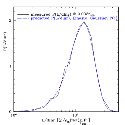
Figure 7: Normalized dark matter annihilation “luminosity” per logarithmic radial interval ($4\pi\rho^{2}(r)r^{3}$) for the full halo sample. The prediction assumes an Einasto profile with a Gaussian concentration scatter, as in Fig. 4.

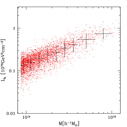
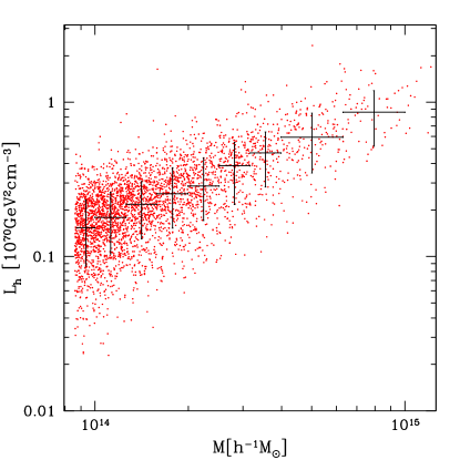
Figure 8: The inferred dark matter luminosities in units of $10^{70}{\mathrm{GeV}^{2}\mathrm{cm}^{-3}}$. Each dot represents a dark matter halo, while the vertical bars represent the 68 percentile of the distribution in each virial mass bin, whose width is denoted by the horizontal bars. Left panel: Luminosity computed directly from the density profile extracted from the simulation for each halo. Right panel: Expected luminosity computed from fitting a concentration to each halo and assuming an Einasto density profile.

In order to assess the origin of the scatter in halo annihilation luminosities and the contribution due to the scatter in concentrations, we compute the dark luminosity of each simulation halo, and compare with the expected luminosity given its measured concentration. We show in Fig. 8 the distribution of halo dark luminosities computed directly from the simulation halo density profile (left panel) together with the prediction of the same quantity from an Einasto profile using the individually measured concentration of each halo (right panel). We bin the data in mass, and determine the mean and 68 percentile of the distribution. The measured and predicted luminosities and 1 $\sigma$ scatter agree well; this suggests that radial correlations in density should not prevent accurate estimation of the annihilation luminosity of a halo.

Thus, the origin of the distribution of luminosities at each mass bin is the distribution in concentrations, which correlate with formation time, albeit with large scatter (see e.g. Neto et al. 2007). The correlation between concentration and annihilation luminosity can be modelled in the following manner for the smooth density component of dark matter halos. The normalization of the profile is proportional to $\rho_{-2}\sim c_{200}^{\gamma}$, where $\gamma~{}\sim 3$ for $c_{200}\gg 1$, and $r_{-2}\sim c_{200}^{-1}$. It follows that, roughly speaking, the luminosity scales as $L\sim\rho_{-2}^{2}r_{-2}^{3}\sim c_{200}^{2\gamma-3}$, leading to $L\sim c_{200}^{3}$ for $c_{200}\gg 1$, although for concentrations typical of our clusters $L\sim c_{200}^{1.5}$. Note that it is difficult to distinguish between the subtle differences between a Gaussian distribution of concentrations and a log-normal one from Fig. 8. In addition, we note that the mean of the luminosity distribution at each mass bin is roughly proportional to the mass of the halo. This is to be expected as the luminosity of a dark matter distribution that is described by a two-parameter profile (e.g., NFW, and/or Einasto) is $L\sim\rho_{-2}^{2}r_{-2}^{3}\sim M^{\beta}$, where $\beta\approx 1$ because the dependence of concentration on mass is relatively weak.

5.2 Cosmological $\gamma$-ray background

We now consider the contribution of the scatter in densities to the cosmological $\gamma$-ray background: the annihilation flux integrated over all halos at all masses and redshifts. We are interested in the effects of the non-universality of profiles to the expected gamma-ray background. In § 4.2, we showed for cluster halos that the distribution in halo concentrations fully describes the distribution in halo densities (at small radii). This enables an accurate estimate of the distribution in dark matter annihilation luminosities (see § 5.1). In order to estimate the dark matter annihilation background, we assume that this holds for halos of all masses at all redshifts.

We compute the gamma-ray background as

$$\frac{dN_{\gamma}}{dEdAdtd\Omega} = \frac{1}{4\pi}\frac{c}{H_{0}}\int_{0}^{\infty}\int_{M_{min}}^{\infty}\frac{\langle\sigma v\rangle}{M_{\chi}^{2}}\frac{dN_{\gamma}}{d[E(1+z)]}$$

$$\times \frac{1}{h(z)}\frac{dn(z)}{dMdV}\int_{0}^{R_{v}}\rho_{M}^{2}(r)d^{3}r\,dM\,dz,$$

where $c$ is the speed of light, $H_{0}=0.7$ is the present value of the Hubble constant, and $h(z)=\sqrt{\Omega_{M}(1+z)^{3}+\Omega_{\Lambda}}$. We assume that $\Omega_{M}=0.27$ and $\Omega_{\Lambda}=0.73$. We use an Einasto density profile parameter of $\alpha=0.1645$, the value for the “typical” halo mass formed from a $1\sigma$ peak in the mass-density field as given in Gao et al. (2008) (and we ignore any mass and redshift dependence of $\alpha$). The quantity $dN_{\gamma}/d[E(1+z)]$ is the spectrum of the emitted photons at a source energy of $E(1+z)$, and the mass function of objects of mass $M$ at redshift $z$ is $dn(z)/dMdV$. We use the mass function of Reed et al. (2007).

We assume that the annihilation proceeds to a $b\bar{b}$ quark final state, and that the distribution in the number of gamma-rays emitted per source energy interval $E_{s}$ are described by the functional form given in Bergstrom, Ullio & Buckley (1998), namely,

$$\frac{dN}{dE_{s}}=\frac{1}{M_{\chi}}\left(\frac{E_{s}}{M_{\chi}}\right)^{-3/2}{\rm exp}\left[-10.7\frac{E_{s}}{M_{\chi}}\right].$$ (9)

We estimate the cosmological gamma-ray background for three different halo concentration distributions. First, we assume an Einasto functional form of the density as a function of radius and a one-to-one dependence of concentrations on mass and redshift as given in Maccio et al. (2007); this is case “Einasto”. However, halo concentrations exhibit a distribution at fixed halo mass and redshift (see § 4.1). As such, we consider a second case, “Einasto $+$ Gaussian”, in which halo concentrations instead follow a Gaussian distribution, given by $\sigma_{G}=0.283c_{200}$, where $c_{200}$ remains the Maccio et al. (2007) concentration as a function of mass and redshift, and the Einasto profile still describes the density distribution. This value for the Gaussian width corresponds to the fractional width found in our halo sample. Finally, we consider case “Einasto $+$ LogNormal” where the concentration distribution is log-normal about the mean concentration value, with dispersion given by $\sigma_{LN}=0.121$, and all other aspects of the background calculation (i.e. Einasto profile, mean concentration-mass-redshift relation) remain the same as the two other cases.

In Fig. 9, we show the expected cosmological gamma-ray background for the three different distributions of dark matter. As expected, in the presence of a spread in the distribution of concentrations, the annihilation flux is increased relative to the case where there is a one-to-one mapping between concentration and mass. We find that a log-normal distribution would give rise to approximately a 10% increase in the annihilation flux relative to our preferred Gaussian distribution of concentrations (which is only a few percent higher than the simple case of no distribution in concentrations).

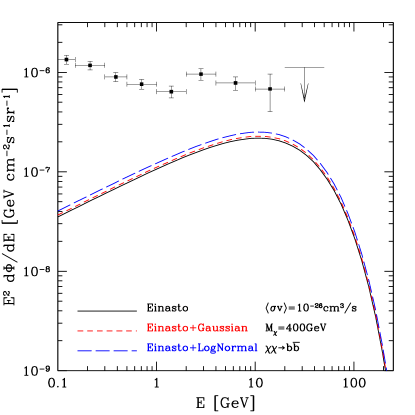
Figure 9: The effects of a Gaussian (short-dashed) and log-normal (long-dashed) distribution of concentration parameters to the cosmological extragalactic dark matter annihilation background. The solid curve represents the background computed by assigning a fixed $c(M)$ relationship without a spread. In all cases, the background is assumed to be due to a 400 GeV WIMP annihilating with a cross section of $10^{-26}{\mathrm{c}m^{3}s^{-1}}$ into a $b\bar{b}$ quark pair. Data points are background measurements from the EGRET satellite (Strong et al. 2004), which could include a contribution from dark matter annihilation.

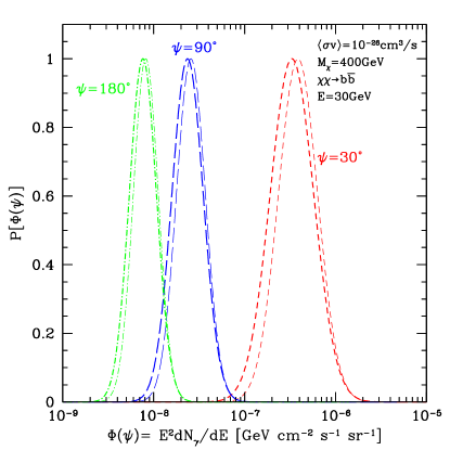
Figure 10: The probability distribution function of gamma-ray flux along a line of sight at $30^{\circ}$ (short-dashed), $90^{\circ}$ (long-dashed) and $180^{\circ}$ (dot-dashed) degrees from the Galactic center for a Gaussian concentration distribution (thick curves) and a log-normal concentration distribution (thin curves). Note the smaller width of the distribution at high Galactic angles relative to the inner parts of the halo. Particle physics parameters are same as Fig. 9.

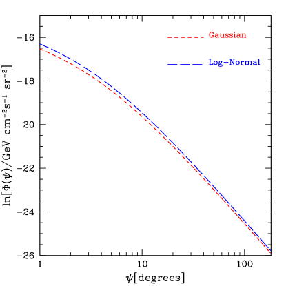
Figure 11: The dependence of the peak of the distributions (Gaussian/log-normal) to the angular distance of the line of sight with the Galactic center. Log-normal distribution in concentrations leads to a slightly higher peak in the flux probability distribution function.

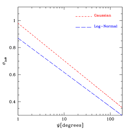
Figure 12: The dependence of the width of the distributions (Gaussian/log-normal) to the angular distance of the line of sight with the Galactic center. Log-normal distribution in concentrations leads to a slightly narrower flux probability distribution function.

5.3 The annihilation flux due to the smooth distribution of dark matter in the Milky Way

We now discuss the impact of the halo density probability distribution function on the Milky Way annihilation flux along different lines of sight. The expected flux at a particular angle $\psi$ with respect to the Galactic center depends on the distribution of dark matter densities along that line of sight. As that is an outcome of the particular concentration of the Galactic Halo, drawn from a distribution of possible concentrations, there is a distribution of expected fluxes for each line of sight. Our calculations of the PDF of dark matter annihilation within the Milky Way assume that the PDF of the spherically-averaged Galactic dark matter density and annihilation are well-described by an Einasto profile and the corresponding PDF of halo concentrations, as we have shown to be the case for cluster-massed halos.

The line of sight flux at an angle $\psi$ with respect to the Galactic center can be written as

$$\frac{dN_{\gamma}(\psi)}{dEdAdtd\Omega}=\frac{1}{4\pi}\frac{\langle\sigma v\rangle}{M_{\chi}^{2}}\frac{dN_{\gamma}}{dE}\,\int_{0}^{\ell_{\rm max}}\rho^{2}_{MW}[r(\ell,\psi)]d\ell,$$ (10)

where $\ell_{\rm max}=d_{\odot}[\cos\psi+\sqrt{(R_{MW}/d_{\odot})^{2}-\sin^{2}\psi}]$ and $r=\sqrt{d_{\odot}^{2}+\ell^{2}-2d_{\odot}\ell\cos\psi}$. We take the distance of the Sun from the Galactic center to be $d_{\odot}=8.5{\rm kpc}$ (consistent with Gillessen et al. 2009), and the radius of the Milky Way halo $R_{200,MW}=250{\rm kpc}$, which implies $M_{200}=1.8\times 10^{12}{\rm{M}}_{\odot}$ and $M_{vir}\simeq=2.\times 10^{12}{\rm{M}}_{\odot}$ (consistent with e.g. Guo et al. 2010). We assume an Einasto profile parameter $\alpha=0.1645$, consistent with that for a halo of Milky Way mass (Gao et al. (2008)).

In Fig. 10, we show the expected flux distribution at various angles with respect to the Galactic center computed using Eq. 10. We calculate the flux distribution for two cases, first where the distribution of concentrations is Gaussian, and second where the distribution of concentrations follows a log-normal distribution. We find that for a log-normal distribution of concentrations the width of the flux distribution along a line of sight is slightly narrower, while at the same time, the mean of the distribution is slightly higher. This is to be expected as the annihilation rate is sensitive to concentration parameter. The high concentration tail of the log-normal concentration distribution contributes to its higher mean flux, while the more extended low concentration range from the Gaussian distribution manifests itself into a broader distribution of fluxes at each particular angular Galacto-centric distance.

It should also be emphasized that the shown distribution functions are uncorrelated, while in reality, because a single concentration must be defined for the Halo, there are correlations between the flux at adjacent angular bins, and anti-correlations between angular values close to zero and 180 degrees. A higher concentration halo has relatively more mass near the center and less near the outer parts. Thus, highly concentrated halos will have higher fluxes with respect to the distribution function toward the Galactic center, and will have relatively smaller fluxes toward the Galactic anti-center.

We now quantify the expected angular dependence of the peak and width of the flux probability distribution function. The peak of the flux distribution is expected to be smaller at high angular distances from the Galactic center. This is a natural consequence of the centrally concentrated spherical distribution of dark matter in a halo, and enables a measure of the underlying density profile of the halo. In Fig. 11, we show the angular dependence of the peak flux. A good fit (within few percent) to this function is obtained by a double power-law as:

$$\ln\bar{\Phi}=a_{1}+a_{2}\ln\psi+a_{3}\ln(a_{4}+\psi)$$ (11)

where the parameters $a_{1}$, $a_{2}$, $a_{3}$ and $a_{4}$ are given in Table 1. The width of the distribution is smaller at large angles from the Galactic center. This is to be expected because the effects of concentration are more apparent in the inner regions of the halo. At radial distances $r\gg r_{-2}$, the changes in the dark matter density due to different halo concentration values are smaller and therefore the flux distribution is narrower. In Fig. 12, we show the expected angular dependence of the width of the flux distribution. We find that a function of the form

$$\sigma=a_{5}\ln\psi+a_{6}$$ (12)

is a good (within few percent) fit to the angular dependence of the width of the distribution function. The quantities $a_{5}$ and $a_{6}$ are given in Table 1. It is important to note here that for large radii ($r\gg r_{-2}$) the halo density PDF that we measured in § 4.2 is larger than inferred from the concentration scatter, which implies that the values of flux uncertainty at large Galacto-centric angles may be larger than our estimates. However, because the Solar Radius is well within $r_{-2}$, the flux should be dominated by the density distribution within $r_{-2}$, even toward the Galactic anti-center, so effects of large radii scatter on the flux PDF should be small.

	$a_{1}$	$a_{2}$	$a_{3}$	$a_{4}$	$a_{5}$	$a_{6}$
${\rm Gaussian}$	-13.70	-0.39	-1.95	3.27	-0.12	0.98
${\rm Log-normal}$	-13.48	-0.40	-1.96	3.22	-0.11	0.87

Table 1: Fitting parameters of Eq. 11 & 12 for the peak and width of the gamma-ray annihilation flux distribution function along a Galactic line of sight.

5.4 Other applications

5.4.1 Cosmological Uncertainty of the Local Dark Matter Density

Applying our results, as before, to a Milky Way mass of $M_{200}=1.8\times 10^{12}{\rm{M}}_{\odot}$, with an ($\alpha=0.1645$) Einasto profile of concentration of $c_{200}=5.97$ (using the concentration-mass relation of Maccio et al. 2008), and a Solar radius of 8.5 kpc implies a Solar radius total matter density of $0.210^{+0.42}_{-0.45}{\rm GeV}\,{\rm cm}^{-3}$ if the concentration PDF is assumed to be Gaussian with width proportional to our values of $\sigma_{c}/c=0.283$. Assumptions of a log-normal distribution of width $\sigma_{LN}=0.121$ results in only minor changes for a local density range of $0.210^{+0.047}_{-0.039}{\rm GeV}\,{\rm cm}^{-3}$, which can be compared with several observational estimates. Bergstrom, Ullio & Buckley (1998) find an allowed range of [0.2-0.8] ${\rm GeV}\,{\rm cm}^{-3}$, and a more recent work by Weber & de Boer (2010) find an acceptable range of [0.2-0.4] ${\rm GeV}\,{\rm cm}^{-3}$. However, tighter constraints are found by Widrow, Pym & Dubinski (2008) and Catena & Ullio (2010), who utilize a variety of dynamical observables to estimate, respectively, $0.304\pm 0.053$ ${\rm GeV}\,{\rm cm}^{-3}$, and $0.385\pm 0.027$ ${\rm GeV}\,{\rm cm}^{-3}$ for the dark matter density. These estimates are somewhat larger than our cosmological range, which hints at the possibility that the Solar radius dark matter density has been enhanced by “adiabatic contraction” in response to baryon cooling.

5.4.2 Implications for Halo Stacking

Our results have implications for many astrophysical applications that depend upon the mass distribution within halos. One such example is the technique of “stacking”halos to improve signal to noise, commonly employed in simulations and observations. In one such application, large numbers of simulated halo density profiles are stacked to measure the mean density profile to high precision (e.g. Gao et al. 2008; Hayashi & White 2008). From an observational perspective, stacking many halos of similar mass greatly reduces the noise in, for example, weak lensing determinations of halo mass profiles and concentrations (e.g. Mandelbaum, Seljak, & Hirata 2008; Mandelbaum et al. 2010; Sheldon et al. 2009ab).

Our results support the viability of halo “stacking”. Due to the fact that the distribution of densities at fixed radius is Gaussian and the distribution of concentrations is also Gaussian, a stacked density profile is indeed an accurate representation of the median profile. This is particularly convenient in that it allows the mean halo profile to be parameterized into an analytic form without bias, and allows unbiased stacking of observational mass profiles. In Fig. 13, we have verified that the cumulative cluster mass distribution also remains unbiased. We compare the Einasto form of a 3-dimensional enclosed mass profile of $c_{200}=4.55$ and $\alpha=0.19$ with the same quantity for a mock stacked halo drawn from a Gaussian distribution of concentrations of mean $c_{200}=4.55$ and scatter $\sigma_{G}=0.283c_{200}$, and find agreement to better than $1\%$, except within a few percent r_vir where differences approach $2\%$. This implies that mass profiles determined by lensing studies should be free from biases associated with halo stacking. Cosmological simulations have been used to demonstrate that accurate three dimensional mass profiles can be constructed from stacked shear signals (e.g. Johnston et al. 2007); our work shows that any potential systematic bias related to the distribution of halo concentrations or densities will be negligible for a gaussian concentration PDF, even for future precision surveys. If, instead, the density distribution had been log-normal, then a stacked halo would have been biased toward higher cumulative masses at small radii, by more than $6\%$ at $1\%$r_vir in our test case.

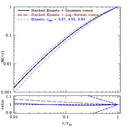
Figure 13: Enclosed mass in spherical shells for mock stacked halo samples with Einasto profile at $c_{200}=4.55$ plus Gaussian concentration distribution and Log-normal concentration distribution. $c_{200}=3.27$ and $c_{200}=5.83$ denote the $1-\sigma$ range in concentration distribution. Bottom panel shows the ratio of each mass profile with respect to mean concentration, $c_{200}=4.55$, Einasto profile. Level of agreement with mean concentration indicates robustness of $M<r$ in stacked halo samples against bias caused by halo-to-halo scatter in concentrations.

6 Limitations of this work

In this work, we do not consider other potential important factors to the annihilation rate, which could possibly be dominant over the halo-to-halo scatter associated with hierarchical structure formation (via the distribution of concentrations) that we have examined. Among them is the amount of substructure in small subhalos and streams (the “clumpy” dark matter component), whose contribution can boost the annihilation rate relative to that of a smooth halo, and will add to the uncertainty in the local dark matter density (e.g. Kamionkowski & Koushiappas 2008; Kamionkowski et al. 2010, Vogelsberger et al. 2009). We also ignore any gravitational coupling that the differential evolution of baryonic halo component may have on the dark matter halo structure. Baryon influences may include gas cooling; this could cause the dark matter halo to respond to the deeper potential by “adiabatic contraction”(Blumenthal et al. 1986). However, strong stellar or AGN feedback could instead lead to shallowing of the dark matter potential (e.g. Duffy et al. 2010). Although these effects may be important, they are beyond the scope of this study.

Our measurements of the cosmological distribution of halo concentrations, densities, and other quantities utilized only clusters from the simulation (because those are the best resolved halos). Our application toward annihilation rates in the Galaxy relies upon the assumption that the behavior of the halo-to-halo profile scatter is similar for galaxies and clusters, namely that the probability distribution of the mean density in radial shells is always described by the Einasto profile with a Gaussian distribution in halo concentrations. The assertion that the distribution of halo concentration remains universally Gaussian, while speculative, is supported by the fact that the logarithmic width and shape of the concentration distribution has weak or no mass or redshift dependence (e.g. Bullock et al. 2001; Neto et al. 2007; Gao et al. 2008; Maccio et al. 2007). This is expected from the self-similar scatter in formation time with mass and the close correlation between formation time and concentration (Wechsler et al. 2002). Additionally, Knollmann, Power & Knebe (2008) used scale-free simulations to show that the scatter in halo profile concentration and density slope has little dependence on matter power spectral index (which varies with halo mass) over a range bracketing well beyond the effective spectral indices of clusters and galaxies. Future studies are warranted utilizing a wider range in halo masses to determine whether the distribution of concentrations is universally Gaussian.

7 Conclusions

The probability distribution function of dark matter within halos, as we have explored in this work, provides some basis for interpreting both indirect and direct dark matter detection experiments in a cosmological context. Constraints upon the dark matter density, particle mass, or the self-annihilation cross section depend on the probability distribution function of dark matter.

Our results indicate that halo concentration is the primary cosmological contributor to the dark matter PDF. This implies a particular correlation between the local dark matter density, relevant for direct detection efforts, and the dark matter density in the direction of the Galactic center (and elsewhere), applicable to indirect detection experiments. The effect of halo concentration should thus be a crucial factor in verifying the consistency of dark matter density constraints made from multiple dark matter detection techniques. Ultimately, dark matter signals might be able to test the validity of the $\Lambda$CDM cosmological model through estimates of the dark density at differing locations within the Milky Way halo, and perhaps also within other halos.

8 acknowledgments

This work was partially supported by the DOE through the IGPP, the LDRD-DR and the LDRD-ER programs at LANL. We thank Carlos Frenk, Tom Theuns, Salman Habib, Katrin Heitmann, and Zarija Lukić for helpful discussions. DR thanks KITP for its hospitality where portions of this work were completed. LG acknowledges support from the one-hundred-talents program of the Chinese academy of science (CAS), the National basic research program of China (program 973 under grant No. 2009CB24901), NSFC grants (Nos. 10973018) and an STFC Advanced Fellowship, as well as the hospitality of the Institute for Computational Cosmology in Durham, UK. We thank the Virgo Consortium for kindly allowing us use of the Millennium simulation. We are grateful to the anonymous referee for insightful suggestions.

References

- Bergstrom, Ullio & Buckley (1998) Bergstrom L., Ullio P., Buckley J., 1998, Astroparticle Phys., 9 137
- Bertone, Hooper & Silk (2005) Bertone G., Hooper D., Silk J., 2005, Phys. Rept., 405, 279
- Blumenthal et al. (1986) Blumenthal G., Faber S., Flores R., Primack J., 1986, ApJ, 301, 27
- Bullock et al. (2001) Bullock J. S., Kolatt T. S., Sigad Y., Somerville, R. S., Kravtsov A. V., Klypin A. A., Primack J. R., Dekel A., 2001a, MNRAS, 321, 559
- Catena & Ullio (2010) Catena R., Ullio P., 2010, JCAP, 08, 004
- Duffy et al. (2008) Duffy A., Schaye J., Kay S., Dalla Vecchia C., 2008, MNRAS, 390, L64
- Duffy et al. (2010) Duffy A., Schaye J., Kay S., Dalla Vecchia C., Booth C., 2010, MNRAS, 405, 2161D
- Einasto (1965) Einasto J., Trudy Inst. Astrofiz. Alma-Ata, 1965, 51, 87
- Eke, Cole, & Frenk (1996) Eke V., Cole S., Frenk C., 1996, MNRAS, 282, 263
- Fukushige, Kawai, & Makino (2004) Fukushige T., Kawai A., Makino J., 2004, ApJ, 606, 625
- Gao & White (2006) Gao L., White S. D. M., MNRAS, 2006, 373, 65
- Gao et al. (2008) Gao L., Navarro J., Cole S., Frenk C. S., White S. D. M., Springel V., Jenkins A., Neto A., 2008, MNRAS, 387, 536
- Gillessen et al. (2009) S.Gillessen, F. Eisenhauer, S. Trippe, T. Alexander, R. Genzel, F. Martins, T. Ott, 2009, ApJ, 692, 1075
- Guo et al. (2010) Guo Q., White S., Li C., Boylan-Kolchin M., 2010, MNRAS, 404, 1111
- Hayashi & White (2008) Hayashi E., White S.D.M., 2008, MNRAS, 388, 2
- Jing (2000) Jing Y., 2000, ApJ, 535, 30
- Johnston et al. (2007) Johnston D., Sheldon E., Tasitsiomi A., Frieman J., Wechsler R., McKay T., 2007, ApJ, 656, 27
- Jungman, Kamionkowski & Griest (1996) Jungman G., Kamionkowski M., Griest K., 1996, Phys. Reports, 267, 195
- Kamionkowski & Koushiappas (2008) Kamionkowski M., Koushiappas S. M., 2008, Phys Rev D, 77, 10, 3509
- Kamionkowski et al. (2010) Kamionkowski, M., Koushiappas, S. M., & Kuhlen, M. 2010, Phys Rev D, 81, 043532
- Knollmann, Power & Knebe (2008) Knollmanns S., Power C., Knebe A., 2008, MNRAS, 385, 545
- Kuhlen, Diemand & Madau (2008) Kuhlen M., Diemand J., Madau P., 2008, ApJ, 686, 262
- Lukić et al. (2009) Lukić Z., Reed D., Habib S., Heitmann K., 2009, ApJ, 692, 217
- Maccio et al. (2007) Maccio A., Dutton A., van den Bosch F., Moore B., Potter D., Stadel J., 2007, MNRAS, 378, 55
- Maccio et al. (2008) Maccio A., Dutton A., van den Bosch F., 2008, MNRAS, 391, 1940
- Mandelbaum, Seljak, & Hirata (2008) Mandelbaum R., Seljak U., Hirata C., 2008, JCAP, 8, 6M
- Mandelbaum et al. (2010) Mandelbaum R., Seljak U., Baldauf T., Smith R., 2010, MNRAS, 405, 2078
- Moore et al. (1998) Moore B., Governato F., Quinn T., Stadel J., Lake G., 1998, AJ, 499, L5
- Navarro, Frenk & White (1996) Navarro J. F., Frenk C. S., White S. D. M., 1996, ApJ, 462, 563
- Navarro, Frenk & White (1997) Navarro J. F., Frenk C. S., White S. D. M., 1997, ApJ, 490, 493
- Navarro et al. (2004) Navarro J. F., et al. , 2004, MNRAS, 349, 1039
- Neto et al. (2007) Neto A., et al. , 2007, MNRAS, 381, 1450
- Power et al. (2003) Power C., Navarro J. F., Jenkins A., Frenk C. S., White S. D. M., Springel V ., Stadel J., & Quinn T., 2003, MNRAS, 338, 14
- Reed et al. (2005) Reed,D., Governato F., Verde L., Gardner J., Quinn T., Merritt D., Stadel J., Lake G., 2005, MNRAS, 357, 82
- Reed et al. (2007) Reed D. S., Bower R., Frenk C. S., Jenkins A., Theuns T., 2007, MNRAS, 374, 2
- Seljak & Zaldarriaga (1996) Seljak U., Zaldarriaga M., 1996, ApJ, 469, 437
- Sheldon et al. (2009) Sheldon E., et al. , 2009a, ApJ, 703, 2217
- Sheldon et al. (2009) Sheldon E., et al. , 2009b, ApJ, 703, 2232
- Springel (2005) Springel V., 2005, MNRAS, 364, 1105
- Springel et al. (2005) Springel V., et al. , 2005, Nature, 435, 629
- Springel et al. (2008) Springel V., et al. , 2008, Nature, 456, 73
- Springel et al. (2008) Springel V., et al. , 2008, MNRAS, 391, 1685
- Strong et al. (2004) Strong A., Moskalenko I., Reimer O., 2004, ApJ, 613, 956
- Weber & de Boer (2010) Weber M., de Boer W., 2010, A&A, 509, 25
- Wechsler et al. (2002) Wechsler R. H., Bullock J. S., Primack J. R., Kravtsov A. V., Dekel A., 2002, ApJ, 568, 52.
- Widrow, Pym & Dubinski (2008) Widrow L., Pym B., Dubinski J., 2008, ApJ, 679, 1239
- Ullio et al. (2002) Ullio P., Bergstrom L., Edsjo J., Lacey C., 2002, Phys. Rev. D, 66, 123502
- Vogelsberger et al. (2009) Vogelsberger M., et al. , 2009, MNRAS, 395,797
- Zavala, Springel & Boylan-Kolchin (2010) Zavala J., Springel V., Boylan-Kolchin M., 2010, MNRAS, 405, 593